Energy-Optimized Longitudinal–Steering Coordinated Torque Vectoring for an In-Wheel-Motor-Driven Electric Vehicle

Abstract

Four-wheel-drive electric vehicles equipped with independently controllable driving, braking, and steering actuators provide additional degrees of freedom for reducing electric-machine and tire-loss energy. This paper presents a real-time longitudinal–steering coordinated torque-vectoring framework for a vehicle driven by four in-wheel motors. A model-predictive active-front-steering controller coordinates the front-wheel steering angle and external yaw moment to reduce steering resistance and lateral tire-slip loss. A reduced inter-axle propulsion problem is analyzed using the Karush–Kuhn–Tucker conditions, and its speed-dependent switching threshold is calibrated offline by particle swarm optimization. Regenerative braking is allocated by an Energy-Optimized Distribution curve subject to ideal-distribution and regulatory constraints. For general positive-torque operation, sequential quadratic programming distributes the four wheel torques by considering motor input power, tire-slip energy, total torque, yaw-moment demand, and actuator limits. Hardware-in-the-loop results under the United States high-acceleration driving cycle and a double-lane-change maneuver show that the proposed strategy reduces energy consumption relative to uniform and tire-utilization-based torque-vectoring strategies.

1. Introduction

Compared with conventional centralized-drive electric vehicles, distributed-drive electric vehicles equipped with independently controllable wheel actuators provide additional degrees of freedom for torque allocation and wheel-loss-energy optimization [1]. When distributed propulsion is coordinated with regenerative braking and electromechanical braking, the multi-actuator system requires more complex braking-force coordination and control allocation [2]. For four-wheel-independent-drive and four-wheel-independent-steering electric vehicles, independent regulation of wheel torque and steering angle further improves yaw and lateral stability control capability [3]. Under extreme operating conditions, the primary objective is to preserve vehicle handling stability and safety margins [4]. In contrast, under normal medium-to-high-friction and low-to-moderate lateral-demand conditions, greater emphasis can be placed on energy optimization while maintaining the required stability constraints [5,6].

Motor-efficiency-oriented torque allocation has been investigated from several complementary perspectives. Pennycott et al. optimized wheel-torque allocation to reduce electric-motor power losses [7]. Chatzikomis et al. developed an energy-efficient torque-vectoring algorithm that considers electric-powertrain efficiency, tire-slip losses, and drivability requirements [8]. Parra et al. formulated a nonlinear model-predictive controller for energy-efficient torque vectoring subject to vehicle-dynamics constraints [9]. Hu et al. employed the Karush–Kuhn–Tucker conditions to identify energy-efficient active-wheel configurations for an electric-wheel-driven vehicle [10]. Tire-energy-oriented studies have instead focused on tire-force distribution and tire-slip-loss minimization. Suzuki et al. investigated tire-force distribution norms, including the minimization of tire workload and tire-slip energy dissipation [11]. Gao et al. incorporated motor losses and tire-slip energy into a unified four-wheel torque-allocation framework [12]. Zhao et al. designed and experimentally evaluated an energy-efficient controller that explicitly considers tire-slip energy [13]. Kobayashi et al. developed a direct-yaw-moment controller that minimizes tire-slip power loss [14]. Najjari et al. integrated constrained active steering and torque vectoring for energy-efficient vehicle-stability control [15]. Choi et al. optimized steering and yaw-moment control inputs to reduce cornering resistance using vehicle-to-vehicle information [16].

Existing studies have therefore emphasized motor-loss minimization, tire-slip-loss minimization, or stability–economy coordination under selected operating conditions [17]. However, many methods optimize only a subset of the relevant energy pathways or are tailored to particular maneuvers, limiting system-level optimization across propulsion, cornering, and regenerative braking. Recent work has further advanced hierarchical stability–economy coordination. Liu et al. developed a friction-aware hierarchy combining vision-dynamics road-friction estimation, adaptive model-predictive direct-yaw control, and quadratic-programming-based torque allocation; an extended phase plane adjusts the relative priority of stability and energy consumption [18]. Janardhanan et al. proposed a linear time-varying model-predictive global force-reference generator and a control allocator for a 4 × 4 heavy electric vehicle with heterogeneous electric machines and friction brakes, explicitly accounting for both operating losses and zero-torque idle losses [19]. These studies primarily address friction-aware stability–economy coordination and energy-efficient allocation for heterogeneous heavy-vehicle powertrains, respectively.

Against this background, the present work focuses on four identical direct-drive in-wheel motors and integrates four physically distinct energy-optimization elements: active-front-steering energy reduction, a speed-dependent active-motor threshold, an energy-oriented regenerative-braking distribution curve, and a four-wheel allocation objective containing both motor input power and longitudinal/lateral tire-slip power. The methodological contribution is the structured integration and validation of these energy pathways within a single real-time framework; the individual optimization tools—model predictive control, fuzzy inference, Karush–Kuhn–Tucker analysis, and sequential quadratic programming—are established methods. Accordingly, a physically structured longitudinal–steering energy-optimization framework is established: active front steering reduces cornering resistance and lateral tire-slip loss; the propulsion-mode layer selects the active motors using a speed-dependent threshold; regenerative braking is distributed under braking-stability constraints; and the general four-wheel allocator jointly considers motor and tire-slip energy.

The remainder of this paper is organized as follows. Section 2 presents the driver, in-wheel-motor, vehicle, and Unitire-based tire-slip-energy models. Section 3 develops the energy-optimized active-front-steering controller. Section 4 formulates the propulsion-mode analysis, regenerative-braking distribution, and sequential-quadratic-programming (SQP)-based coordinated torque-vectoring strategy. Section 5 presents offline simulations and hardware-in-the-loop validation under longitudinal and steering conditions. Section 6 summarizes the main findings and limitations.

2. System Modeling

2.1. Model of the Four-Wheel-Drive Electric Vehicle

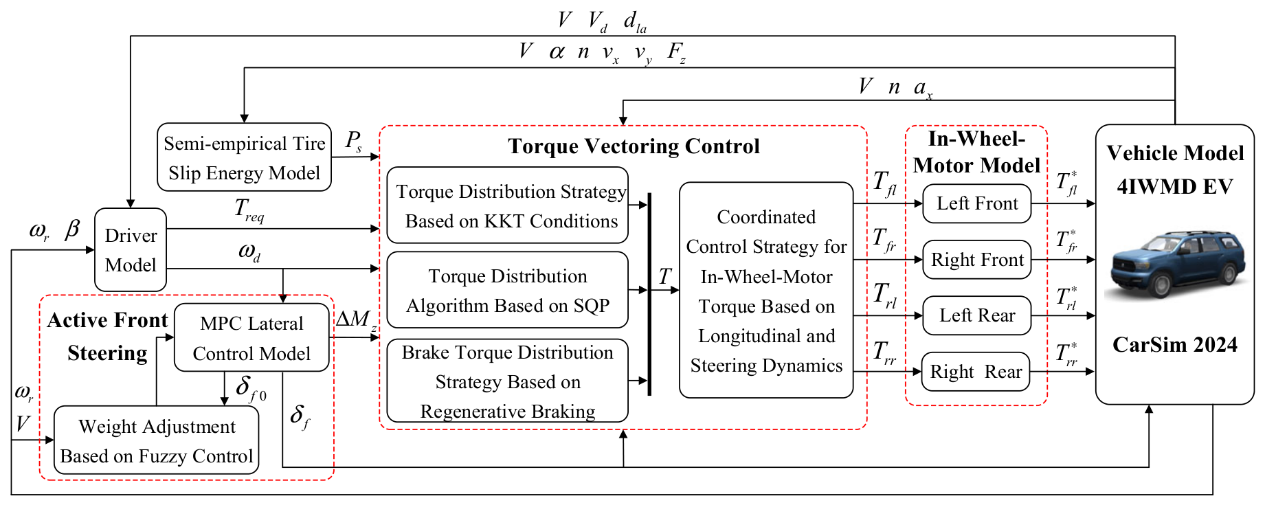
A full-size sport utility vehicle (SUV) model is established in CarSim and modified to represent the powertrain, steering system, body, suspension, and tires of the studied four-wheel-drive electric vehicle (4WD-EV). The main vehicle parameters are listed in

Table 1. Main vehicle parameters.

Symbol	Description	Value
$m$	Vehicle mass	2607 (kg)
$I_z$	Moment of inertia about yaw	3525 (kg·m2)
$d$	Tread width of vehicle	1.725 (m)
$l_f$	Distance from CG to front axle	1.46 (m)
$l_r$	Distance from CG to rear axle	1.65 (m)
$R_e$	Effective rolling radius of wheel	0.384 (m)
Tire	Tire specification	235/65 R17

. The driver, in-wheel-motor, and Unitire semi-empirical tire models are im-plemented in MATLAB/Simulink R2023a and coupled with the CarSim vehicle model. The overall control architecture is shown in Figure 1.

The studied vehicle is equipped with four liquid-cooled, outer-rotor, direct-drive Elaphe in-wheel motors and a steer-by-wire four-wheel-steering system, the vehicle parameters are shown in Table 1. Because the present study addresses energy optimization within the normal stability region, only active front steering (AFS) is used in the control framework.

2.2. Driver Model

The longitudinal driver model regulates the difference between the reference vehicle speed $v_{\mathrm{r}\mathrm{e}\mathrm{f}}$ and the actual vehicle speed $v$. A proportional–integral–derivative (PID) controller computes the total demanded wheel torque $T_{\mathrm{r}\mathrm{e}\mathrm{q}}$ using Equation (1). The controller gains were determined by sequential empirical tuning in the Simulink vehicle model: the proportional action was adjusted to obtain the required acceleration response without sustained oscillation, the integral action was adjusted to eliminate steady-state tracking error, and the derivative action was used to suppress torque fluctuation during rapid acceleration and deceleration.

$$T_{req}=K_p\cdot e\left(t\right)+K_i\cdot {\displaystyle \int e\left(t\right)dt}+K_d\cdot {\displaystyle \frac{de\left(t\right)}{dt}}$$

(1)

where K_p, K_i, and K_d denote the proportional, integral, and derivative gains, respectively. The vehicle-speed error is e(t) = v_ref(t) − v(t). The implemented gains are K_p = 520, K_i = 45, and K_d = 18. The controller gains were obtained through a staged engineering calibration procedure. First, the integral and derivative gains were set to zero, and the proportional gain was gradually increased until the required acceleration response was achieved without sustained oscillation. Second, the integral gain was progressively introduced to eliminate the steady-state speed-tracking error under driving-cycle conditions. Third, the filtered derivative term was added to suppress demanded-torque oscillations during rapid transitions between acceleration and deceleration. Finally, torque saturation and an anti-windup mechanism were implemented to prevent continued integrator accumulation when the demanded torque exceeded the available capability of the four in-wheel motors.

The final parameter set was evaluated using the completed 0–100 km/h acceleration case and the US06 driving cycle. The speed overshoot in the acceleration case remained below 0.4%, and the root-mean-square speed-tracking error under the US06 cycle was approximately 0.31 m/s. No sustained oscillation or windup-induced divergence caused by output saturation was observed.

Other implementation parameters, including the motor response time, driver preview time, MPC prediction and control horizons, fuzzy-set parameters, particle-swarm-optimization settings, motor operating boundaries, tire-model coefficients, braking thresholds, and hardware-in-the-loop settings, are provided or cross-referenced in the corresponding sections, as shown in

Table 2. Longitudinal driver-controller specification and parameter provenance.

Item	Specification	Implementation/Verification
Control law	Proportional–integral–derivative controller	Equation (1)
Tuning method	Sequential empirical calibration	Acceleration response, steady-state tracking error, and torque fluctuation
Validation result	Acceleration overshoot < 0.4%	Completed 0–100 km/h model-validation case
Numerical gain set	Provided with the executable controller model upon reasonable request	Implemented Simulink parameter file

.

To suppress high-frequency noise amplification in the derivative channel, the ideal derivative action in Equation (1) is implemented using the first-order filtered form in Equation (2):

$$D\left(s\right)=K_d{\displaystyle \frac{N_{d}s}{s+N_d}}E\left(s\right)$$

(2)

where $E\left(s\right)$ is the Laplace transform of the vehicle-speed error e(t), $D\left(s\right)$ is the filtered derivative contribution, $K_d$ is the derivative gain defined in Equation (1), and $N_d$ is the derivative-filter coefficient. The implemented value is $N_d$ = 20.

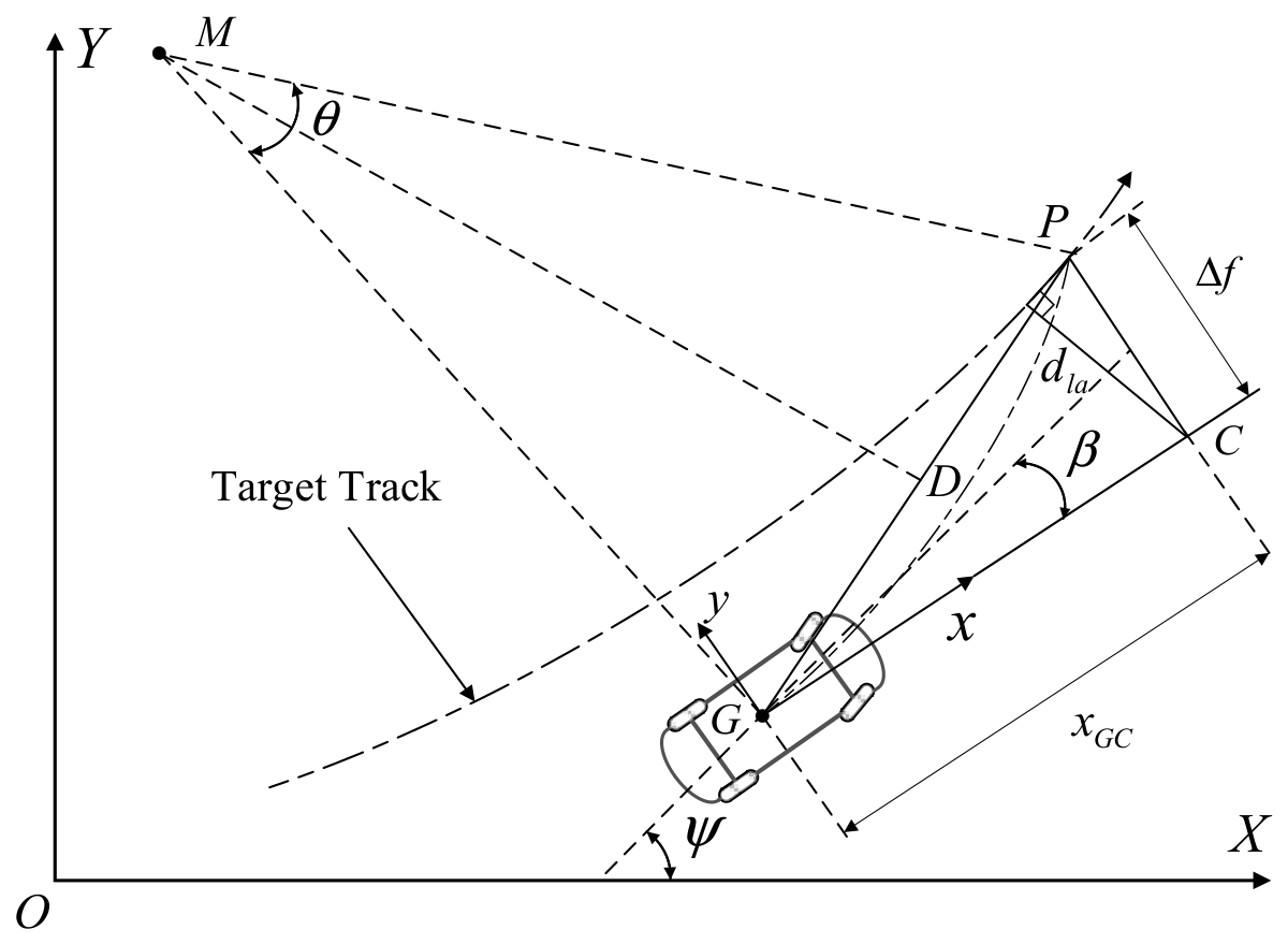
The desired yaw rate is generated by a lateral driver model based on a single-point preview formulation, which approximates the driver response to the target path. The corresponding geometric relationship is shown in Figure 2.

Assuming that the vehicle performs uniform circular motion around point $M$ within the future preview time $t_p$, the lateral trajectory deviation $\Delta f$ is defined as the distance between the preview point $C$ and the target point $P$ on the desired path. Let $d_{la}$ denote the perpendicular projection distance from the preview point to the desired trajectory; this value is obtained from CarSim output. $x_{GC}$ represent the preview distance. Based on the geometric relationships illustrated in the figure, the following equation can be derived:

$$\Delta f={\displaystyle \frac{d_{la}}{\cos \left(\arcsin \left(\frac{d_{la}}{x_{GC}}\right)\right)}}$$

(3)

$${\omega }_d={\displaystyle \frac{2\arctan \left(\frac{\Delta f}{x_{GC}}\right)-2\beta }{t_p}}$$

(4)

2.3. In-Wheel-Motor Model

In the motor model, only the energy-consumption characteristics and torque-response dynamics are considered, whereas detailed electromagnetic dynamics are omitted. The empirical in-wheel-motor (IWM) input-power model is constructed from the measured motor efficiency map and the identified torque-response data [20]. The in-wheel-motor torque response is represented by a first-order transfer function.

$$G\left(s\right)={\displaystyle \frac{T^{\ast }}{T}}={\displaystyle \frac{1}{{\tau }_{d}s+1}}$$

(5)

In this context, $G\left(s\right)$ denotes the transfer function of the motor torque, $T$ represents the torque computed by the torque vectoring control algorithm, and $T^{\ast }$ is the actual output torque from the in-wheel motor model. The parameter ${\tau }_d$ corresponds to the response coefficient of the in-wheel-motor. The power expression of the in-wheel-motor is given as follows:

$$\begin{array}{ll}{P}_{in}={\displaystyle \frac{P_{out}}{\eta }}={\displaystyle \frac{Tn}{9550\cdot \eta }}\hspace{1em}\hspace{1em}& , T>0\\ P_{in}=P_{out}\cdot \eta ={\displaystyle \frac{Tn}{9550}}\cdot \eta \hspace{1em}\hspace{1em}& , T<0\end{array}$$

(6)

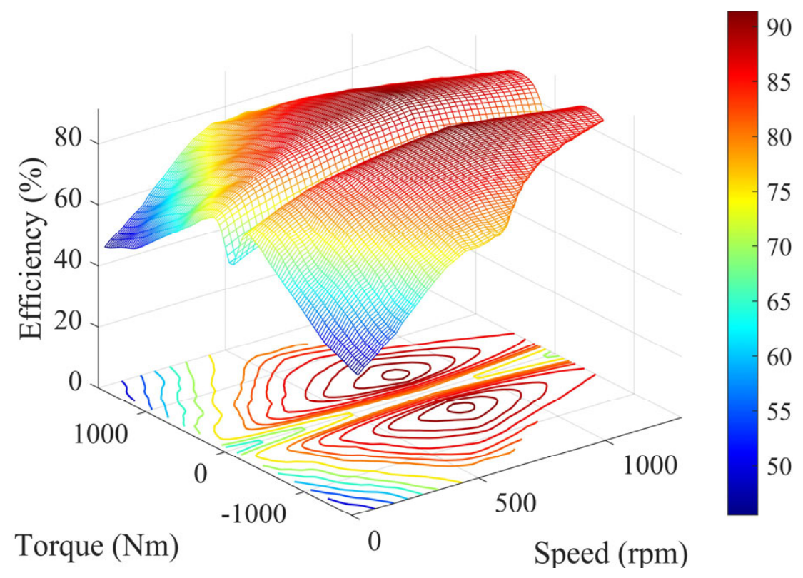
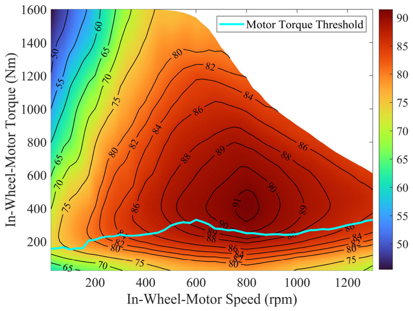
Energy losses occur in both propulsion and regenerative operation because the motor efficiency varies with torque and speed. As shown in Figure 3, the in-wheel motor has comparatively low efficiency in the low-speed and low-torque region.

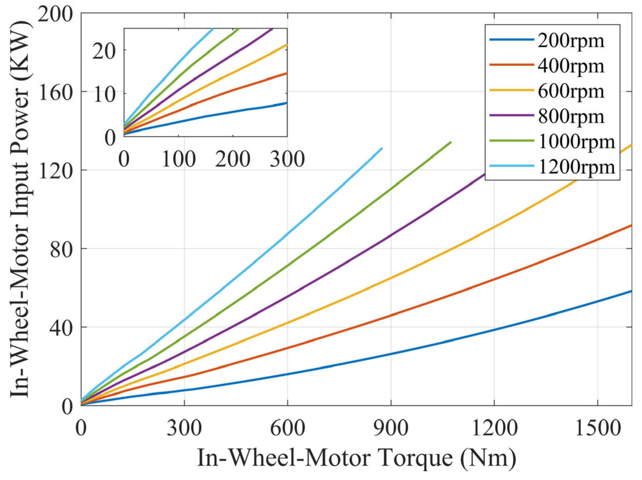
The motor efficiency is represented as a function of torque T and speed n. Accordingly, the electrical input power is fitted at each speed by the cubic polynomial in Equation (7).

$$P_{in}\left(T,n\right)=a\left(n\right)T^3+b\left(n\right)T^2+c\left(n\right)T+d\left(n\right)$$

(7)

In the equation, parameters $a\left(n\right)$, $b\left(n\right)$, $c\left(n\right)$, and $d\left(n\right)$ are speed-dependent power fitting coefficients. Parameter $d\left(n\right)$ represents the additional power loss of the in-wheel motor when the wheel is operating as a passive wheel. This loss is 0 when the motor speed is 0 and increases strictly with the rise in motor speed. A conventional second-order Willans-type polynomial can represent approximately constant, linear, and current-dependent losses at a fixed speed. However, after symmetric front–rear torque substitution, its curvature with respect to the inter-axle transfer variable is independent of the total demanded torque and therefore cannot express the demand-dependent transition observed between single-axle and four-wheel propulsion. The third-order term is introduced as an empirical curvature correction: it preserves the quasi-convex shape of the calibrated input-power curve over the positive-torque interval and yields the demand-dependent curvature coefficient used in the analytical threshold derivation. It is not interpreted as an additional independent physical loss mechanism and is used only within the calibrated motor-map range.

Table 3. Analytical comparison of second- and third-order fixed-speed motor input-power representations.

Model	Fixed-Speed Input-Power Form	Curvature After Symmetric Axle Allocation	Mode-Switch Implication
Second-order Willans type	$P_{\mathrm{i}\mathrm{n},2}\left(T,n\right)=b_2\left(n\right)T^2+c_2\left(n\right)T+d_2\left(n\right).$	$J_2\left(\tau ,n\right)=C_2\left(n,T_{\mathrm{r}\mathrm{e}\mathrm{q}}\right)+b_2\left(n\right){\tau }^2.$	Curvature sign is independent of T_req; no demand-dependent analytical threshold
Third-order empirical model	$P_{\mathrm{i}\mathrm{n},3}\left(T,n\right)=a\left(n\right)T^3+b\left(n\right)T^2+c\left(n\right)T+d\left(n\right)$	$J_m\left(\tau ,n\right)=C\left(n,T_{\mathrm{r}\mathrm{e}\mathrm{q}}\right)+\left[{\displaystyle \frac{3}{4}}a\left(n\right)T_{\mathrm{r}\mathrm{e}\mathrm{q}}+b\left(n\right)\right]{\tau }^2.$	Supports the speed- and demand-dependent switching condition in Equation (44)

summarizes this analytical distinction, and the motor-map identification and propulsion-threshold calibration settings are summarized in

Table 4. Motor-map identification and propulsion-threshold calibration settings.

Item	Setting/Source	Role in the Model
Motor data source	Calibrated Elaphe efficiency map and identified torque-response data	Construction of P_in(T,n) and the first-order torque response
Input-power approximation	Third-order polynomial at each calibrated speed	Local empirical representation within the positive-torque map
Coefficient identification	Least-squares fitting	Determination of a(n), b(n), c(n), and d(n)
Threshold speed grid	25 rpm over 25–1300 rpm	Offline threshold calibration and online lookup
PSO torque-search interval	1–1500 N·m	Crossing search between single-axle and four-wheel input powers
PSO parameters	c1 = c2 = 1.49; inertia weight 0.9 → 0.4; 20 iterations	Offline threshold-calibration settings
Online implementation	One-dimensional lookup with linear interpolation	Real-time propulsion-mode selection
Complete coefficient array	Available from the corresponding author upon reasonable request	Calibrated motor-map data

.

$$P_{\mathrm{i}\mathrm{n},2}\left(T,n\right)=b_2\left(n\right)T^2+c_2\left(n\right)T+d_2\left(n\right)$$

(8)

For implementation, the motor input-power coefficients are identified by least-squares fitting on the calibrated motor-speed grid. The propulsion threshold is evaluated offline at 25 rpm intervals. Online control uses only the calibrated one-dimensional threshold table and linear interpolation; the corresponding identification and calibration settings are summarized in Table 4.

$$\begin{array}{c}q\left(n\right)=q\left(n_j\right)+{\displaystyle \frac{n-n_j}{n_{j+1}-n_j}}\left[q\left(n_{j+1}\right)-q\left(n_j\right)\right],\\ q\in \{a,b,c,d\}, n\in \left[n_j,n_{j+1}\right]\end{array}$$

(9)

2.4. The Semi-Empirical Unitire Tire Model

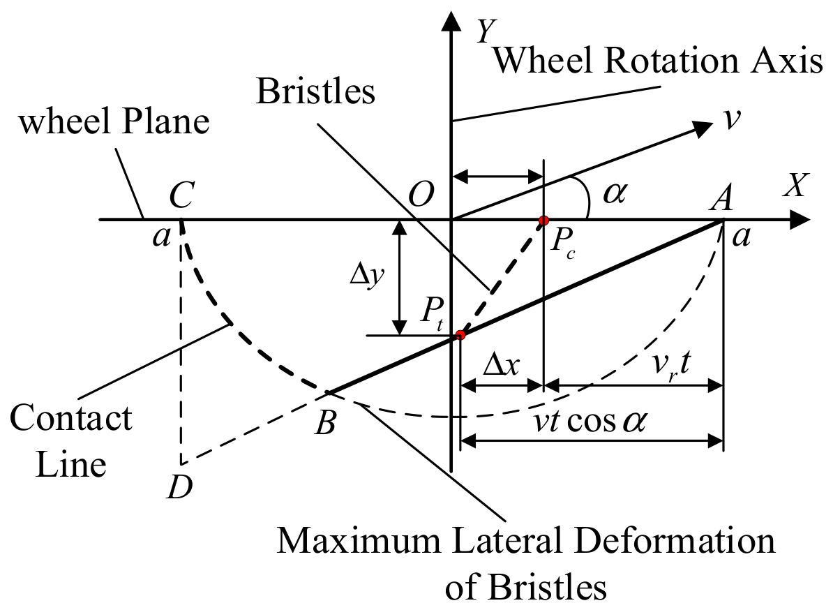
Tire-slip energy is generated by the simultaneous action of slip force and slip ve-locity. A semi-empirical slip-energy model is therefore constructed from the Unitire tire model [21]. Figure 4 illustrates the bristle deformation within the tire contact patch.

The longitudinal and lateral forces of Unitire tires under composite driving conditions are expressed as follows:

$$\begin{array}{l}\overline{F}=1-\exp \left[-\varphi -E{\varphi }^2-\left(E^2+{\displaystyle \frac{1}{12}}\right){\varphi }^3\right]\\ F_x=\overline{F}{\displaystyle \frac{{\varphi }_x}{\varphi }}{\mu }_x{F}_z\\ F_y=\overline{F}{\displaystyle \frac{{\varphi }_y}{\varphi }}{\mu }_y{F}_z\end{array}$$

(10)

Here, $\overline{F}$ denotes the dimensionless tire force. Terms $S_x$ and $S_y$ represent the longitudinal slip ratio and lateral slip ratio of the tire, respectively, which are expressed as follows:

$$S_x={\displaystyle \frac{-v_{sx}}{\omega R_e}}={\displaystyle \frac{\omega R_e-v_x}{\omega R_e}}, S_y=\left(S_x-1\right)\cdot \tan \alpha$$

(11)

Here, $\omega$ denotes the wheel angular velocity, $\alpha$ the tire slip angle, $R_e$ the tire rolling radius, $v_{sx}$ the longitudinal slip velocity at the wheel center, and $v_x$ the longitudinal velocity at the wheel center. In tire testing and tire-model data exchange, the longitudinal slip ratio is also commonly defined according to the Tyre Data Exchange Format (TYDEX) convention as follows:

$$\kappa =-{\displaystyle \frac{V_x-\omega R_e}{V_x}}.$$

(12)

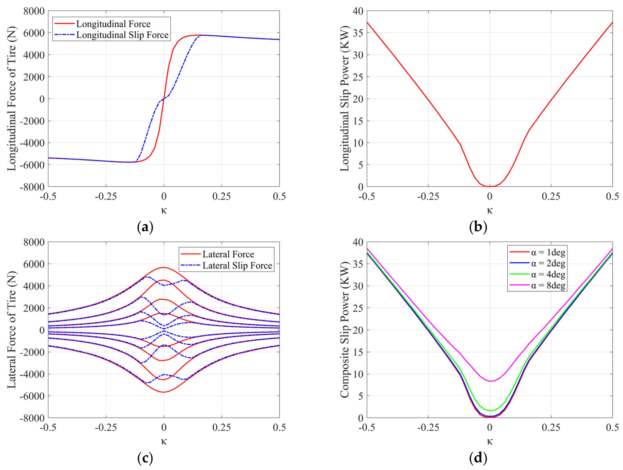
Therefore, the relational expression $S_x=\kappa /1+\kappa$ can be obtained. For clearer observation of the curve, this paper adopts the TYDEX longitudinal slip ratio $\kappa$ as the standard for plotting.

The relative longitudinal slip ratio ${\varphi }_x$, relative lateral slip ratio ${\varphi }_y$, and relative combined slip ratio $\varphi$ in Equation (10) are expressed as follows:

$${\varphi }_x={\displaystyle \frac{K_x{S}_x}{{\mu }_x{F}_z}}, {\varphi }_y={\displaystyle \frac{K_y{S}_y}{{\mu }_y{F}_z}}, \varphi =\sqrt{{\varphi }_x^2+{\varphi }_x^2}$$

(13)

In Equation (14), $K_x$ and $K_y$ represent the longitudinal and lateral stiffness of the tire, respectively. To describe the effect of vertical load variation on the longitudinal and lateral stiffness, the expressions for the tire longitudinal and lateral stiffness are given as follows:

$$\begin{array}{l}{K}_x={\displaystyle \frac{F_z}{l_1^2+l_2^2{F}_{zn}+l_3^2{F}_{zn}^2}}\\ K_y={\displaystyle \frac{F_z}{s_1^2+s_2^2{F}_{zn}+s_3^2{F}_{zn}^2}}\end{array}$$

(14)

In the equation, $F_z$ denotes the tire vertical load, $F_{zn}=F_z/F_{z0}$ represents the dimensionless vertical load ratio, $F_{z0}$ is the static vertical tire load, and $l_1$, $l_2$, $l_3$, $s_1$, $s_2$, and $s_3$ are model parameters. To identify the parameters of the semi-empirical Unitire model, a 235/65 R17 tire available in CarSim and having characteristics close to those of the tire used on the investigated vehicle was selected for virtual tire testing. Under pure longitudinal slip, the test speed was 50 km/h, the longitudinal slip ratio was varied from κ = 0 to κ = 0.5, and the longitudinal force was fitted at vertical loads of 2000, 4000, 6000, 8000, and 10,000 N. Under combined slip, the speed remained 50 km/h, κ was fixed at 0.2, the tire slip angle was varied from α = 0° to α= −20°, and the lateral force was fitted under the same five vertical loads. The resulting comparisons show that the identified Unitire model reproduces the longitudinal-slip and lateral-force characteristics over the investigated load range. The identified axle-specific stiffness coefficients are listed in

Table 5. Identified Unitire stiffness parameters for the 235/65 R17 CarSim tire.

Axle	F_z0 (N)	l1	l2	l3	s1	s2	s3
Front	6784.71	0.2091	0.08907	0.007795	0.2745	5.3 × 10−5	2.33 × 10−4
Rear	6003.44	0.2091	0.08378	0.006897	0.2745	4.3 × 10−5	1.94 × 10−4

, and the fitting comparisons are shown in Figure 5.

$$K_x={\displaystyle \frac{F_z}{l_1^2+l_2^2{F}_{zm}+l_3^2{F}_{zm}^2}}$$

(15)

$$K_y={\displaystyle \frac{F_z}{s_1^2+s_2^2{F}_{zm}+s_3^2{F}_{zm}^2}}$$

(16)

$$F_{zm}={\displaystyle \frac{F_z}{F_{z0}}}$$

(17)

The longitudinal and lateral friction coefficients ${\mu }_x$ and ${\mu }_y$ are calculated using the modified Savkoor formulation in Equation (18) [22].

$$\begin{array}{l}{\mu }_d={\mu }_s+\left({\mu }_m-{\mu }_s\right)\\ \exp \left\{-{\mu }_h^2\log \left[\left|{\displaystyle \frac{v_s}{v_{sm}}}\right|+N\exp \left(-\left|{\displaystyle \frac{v_s}{v_{sm}}}\right|\right)\right]\right\}\end{array}$$

(18)

In Equation (18), ${\mu }_d$ is the dynamic friction coefficient, ${\mu }_m$ is the peak value, ${\mu }_s$ is the full-slip value, ${\mu }_h$ governs the transition shape, $N$ governs the low-slip growth rate, and $v_{sm}$ is the slip speed corresponding to peak friction. The adopted values are ${\mu }_m$ = 1.0, ${\mu }_s$ = 0.75, ${\mu }_h$ = 1.0, and $N$ = 0.8. The longitudinal and lateral peak-friction slip speeds are 2.6 m/s and 0.6 m/s, respectively. These values and the stiffness coefficients in Table 5 are identification parameters of the selected CarSim tire dataset rather than universal Unitire constants.

The total slip force within the tire contact patch can be expressed as:

$$\begin{array}{l}{F}_s={\displaystyle \frac{1}{4}}\mu F_z\left(2+3\xi -{\xi }^3\right)\\ \xi ={\displaystyle \frac{2}{3}}\varphi -1\end{array}$$

(19)

The equivalent friction coefficient $\mu$ along the resultant force direction is given by Equation (20).

$$\mu =\sqrt{{\left({\displaystyle \frac{{\varphi }_x}{\varphi }}{\mu }_x\right)}^2+{\left({\displaystyle \frac{{\varphi }_y}{\varphi }}{\mu }_y\right)}^2}$$

(20)

Based on the above equations, the longitudinal slip force $F_{sx}$, longitudinal slip velocity $v_{sx}$, lateral slip force $F_{sy}$, and lateral slip velocity $v_{sy}$ within the tire contact patch can be obtained, which further allows the calculation of the longitudinal slip power $P_{sx}$ and lateral slip power $P_{sy}$, as shown below:

$$P_{sx}=-F_{sx}{v}_{sx}=F_{s}v\hspace{0.17em}{\displaystyle \frac{S_x}{\sqrt{S_x^2+S_y^2}}}\hspace{0.17em}{\displaystyle \frac{S_x}{1-S_x}}\mathrm{c}\mathrm{o}\mathrm{s}\alpha$$

(21)

$$P_{sy}=-F_{sy}{v}_{sy}=F_{s}v\hspace{0.17em}{\displaystyle \frac{S_y}{\sqrt{S_x^2+S_y^2}}}\hspace{0.17em}{\displaystyle \frac{S_y}{1-S_x}}\mathrm{c}\mathrm{o}\mathrm{s}\alpha$$

(22)

3. Energy-Optimized Active Front Steering

3.1. Model Predictive Control

A linear two-degree-of-freedom model describing lateral and yaw motion is used as the prediction model for the model predictive control (MPC) [23]. The model includes the front-axle steering angle and the externally generated yaw moment, as expressed in Equation (23).

$$\begin{array}{l}m\left({\dot{V}}_y+V{\omega }_r\right)=\left(k_f+k_r\right)\beta +{\displaystyle \frac{{\omega }_r}{V}}\left(l_f{k}_f-l_r{k}_r\right)-k_f{\delta }_f\\ I_z{\dot{\omega }}_r=\left(l_f{k}_f-l_r{k}_r\right)\beta +{\displaystyle \frac{{\omega }_r}{V}}\left(l_f^2{k}_f+l_r^2{k}_r\right)-l_f{k}_f{\delta }_f+\Delta M_z\end{array}$$

(23)

In Equation (23), ${\delta }_f$ is the front-axle steering angle and $\Delta M_z$ is the external yaw moment.

The MPC determines ${\delta }_f$ and $\Delta M_z$ while maintaining trajectory tracking. Penalizing the steering angle and coordinating the external yaw moment reduce cornering resistance and lateral tire-slip loss. The state-space model is written as Equation (24).

$$\dot{x}\left(t\right)=Ax\left(t\right)+Bu\left(t\right)$$

(24)

Here,

$$x\left(t\right)=\left[\begin{array}{c}\beta \\ {\omega }_r\end{array}\right], u\left(t\right)=\left[\begin{array}{c}{\delta }_f \\ \Delta M_z\end{array}\right], A=\left[\begin{array}{cc}{\displaystyle \frac{K_f+K_r}{m{V}_x}}& {\displaystyle \frac{l_f{K}_f-l_r{K}_r}{m{V}_x^2}}\\ {\displaystyle \frac{l_f{K}_f-l_r{K}_r}{I_z}}& {\displaystyle \frac{{l_f}^2{K}_f+{l_r}^2{K}_r}{I_z{V}_x}}\end{array}\right], B=\left[\begin{array}{cc}{\displaystyle \frac{-K_f}{m{V}_x}}& 0\\ {\displaystyle \frac{-l_f{K}_f}{I_z}}& {\displaystyle \frac{1}{I_z}}\end{array}\right]$$

Let the prediction horizon and control horizon be defined as $n$ and $m$ sampling intervals, respectively, subject to the condition $m\le n$. The recursive formulation of the predicted outputs is constructed in the state-space form:

$$Y_n\left(k+1|k\right)=S_{x}X\left(k\right)+S_{u}U\left(k\right)$$

(25)

Here,

$$\begin{array}{c}{Y}_n\left(k+1|k\right)={\left[\begin{array}{c}y\left(k+1|k\right)\\ y\left(k+2|k\right)\\ ⋮\\ y\left(k+n|k\right)\end{array}\right]}_{n\times 1},U\left(k\right)={\left[\begin{array}{c}u\left(k\right)\\ u\left(k+1\right)\\ ⋮\\ u\left(k+m-1\right)\end{array}\right]}_{m\times 1},\\ S_x={\left[\begin{array}{c}A\\ {\displaystyle \sum _{i=1}^2{A}^i}\\ ⋮\\ {\displaystyle \sum _{i=1}^n{A}^i}\end{array}\right]}_{n\times 1},S_u={\left[\begin{array}{cccc}B& 0 & \dots & 0\\ {\displaystyle \sum _{i=1}^2{A}^{i-1}B}& B& \dots & 0 \\ ⋮& ⋮& \ddots & 0 \\ {\displaystyle {\displaystyle \sum _{i=1}^m}{A}^{i-1}B}& {\displaystyle {\displaystyle \sum _{i=1}^{m-1}}{A}^{i-1}B}& \cdots & B\end{array}\right]}_{n\times m}\end{array}$$

The objective function is defined as the cumulative squared deviation between the desired and actual outputs, combined with the cumulative squared control inputs. Specifically, the desired outputs refer to the target yaw rate ${\omega }_d$ and the target vehicle sideslip angle ${\beta }_d$, ${\beta }_d=0$. The optimization objective function can be expressed as follows:

$$\begin{array}{l}\min J={‖{\mathrm{\Gamma }}_y\left(R\left(k+1|k\right)-Y_n\left(k+1|k\right)\right)‖}^2\\ +{‖{\mathrm{\Gamma }}_{u}U\left(k\right)‖}^2\end{array}$$

(26)

Here,

$$\begin{array}{l}{\mathrm{\Gamma }}_y={\left[\begin{array}{l}{w}_y\\ ⋮\\ w_y\end{array}\right]}_{n\times 1}, {\mathrm{\Gamma }}_u={\left[\begin{array}{l}{w}_u\\ ⋮\\ w_u\end{array}\right]}_{m\times 1}, \\ w_y=diag\left\{w_{\beta },w_{{\omega }_r}\right\}, w_u=diag\left\{w_{\delta },w_{\Delta M_z}\right\}\end{array}$$

$R\left(k+1|k\right)$ represents the desired system matrix, while ${\mathrm{\Gamma }}_y$ and ${\mathrm{\Gamma }}_u$ denote the weighting penalty matrices for state deviation and control input, respectively. $w_y$ and $w_u$ are the weighting matrices for output deviation and control input. The above optimization objective function is then formulated as a quadratic programming problem:

$$\min J={\displaystyle \frac{1}{2}}U{\left(k\right)}^{T}HU\left(k\right)+f^{T}U\left(k\right)$$

(27)

Here,

$$\begin{array}{l}H=2\left(S_u^T{\mathrm{\Gamma }}_y^T{\mathrm{\Gamma }}_y{S}_u+{\mathrm{\Gamma }}_u^T{\mathrm{\Gamma }}_u\right), \\ f=-2S_u^T{S}_u{\mathrm{\Gamma }}_y^T{\mathrm{\Gamma }}_{y}Q\left(k+1|k\right),\\ Q\left(k+1|k\right)=R\left(k+1|k\right)-S_x\Delta x\left(k\right)-S_{y}y\left(k\right)\end{array}$$

Only the first element of the optimized control sequence is applied at the current sampling instant, as expressed in Equation (28).

$$u\left(k\right)={\left[I_2 0 \cdots 0\right]}_{1\times m}U\left(k\right)$$

(28)

Due to the different turning radii of the left and right front wheels, applying the same steering angle to both will increase lateral tire slip loss. Therefore, this paper adopts the Ackermann steering geometry to calculate the steering angles of the left and right front wheels based on the front axle steering angle [24]:

$${\delta }_1=\arctan \left({\displaystyle \frac{l}{\frac{l}{\tan {\delta }_f}-\frac{d}{2}}}\right),{\delta }_2=\arctan \left({\displaystyle \frac{l}{\frac{l}{\tan {\delta }_f}+\frac{d}{2}}}\right)$$

(29)

where ${\delta }_1$ denotes the steering angle of the left front wheel, ${\delta }_2$ denotes the steering angle of the right front wheel, and $l=l_f+l_r$ represents the wheelbase of the vehicle.

3.2. Fuzzy Control

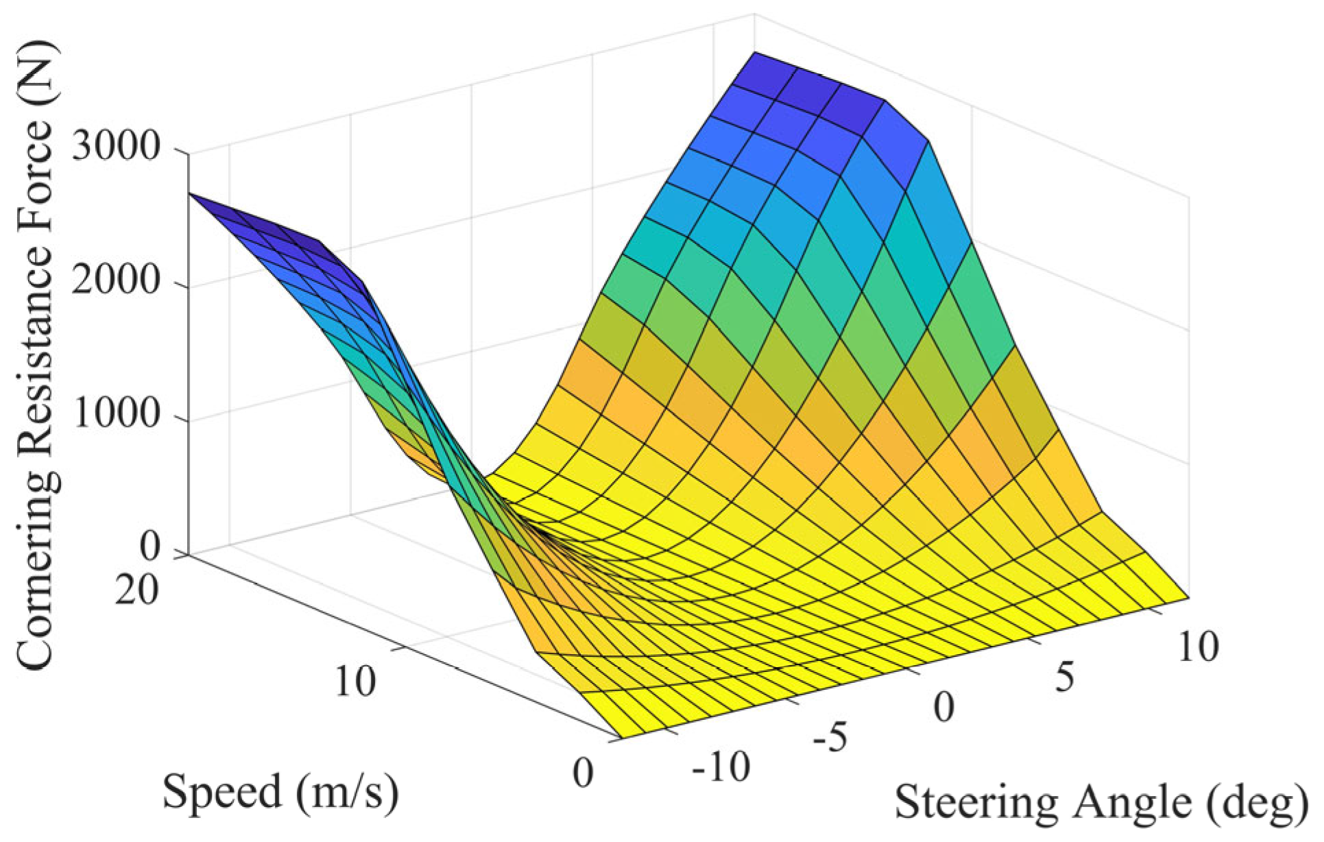
During cornering, the lateral tire forces generate a component opposite to the direction of travel, producing cornering resistance. Earlier formulations based on a two-degree-of-freedom model neglected longitudinal dynamics and the explicit steering-angle effect [25]. The three-degree-of-freedom expression adopted here is given by Equation (30) [26].

$$F_{cr}=-m{\displaystyle \frac{V^2}{R}}\left({\displaystyle \frac{l_r}{l}}{\alpha }_f+{\displaystyle \frac{l_f}{l}}{\alpha }_r\right)$$

(30)

Equation (30) shows that cornering resistance increases with vehicle speed and tire slip angle; the latter is directly affected by the front-wheel steering angle. The resulting cornering-resistance relationship is shown in Figure 6.

The state-tracking weights are fixed at values higher than the control-input weights to preserve trajectory tracking. The steering-angle and external-yaw-moment penalties are adjusted online by the fuzzy controller.

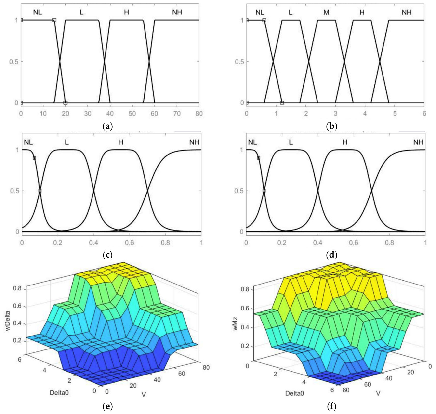
The two fuzzy inputs are vehicle speed and the absolute value of the front-wheel steering angle calculated at the preceding control instant. The vehicle-speed universe is 0–80 km/h and uses four linguistic sets, VL, L, H, and VH. The steering-angle uni-verse is 0–6° and uses five linguistic sets, VL, L, M, H, and VH. Trapezoidal member-ship functions are used with the breakpoints listed in

Table 6. Input membership-function parameters of the fuzzy controller.

Variable	VL	L	M	H	VH
Vehicle speed (km/h)	trap(0,0,15,20)	trap(15,20,35,40)	—	trap(35,40,55,60)	trap(55,60,80,80)
|${\delta }_f$ (k − 1)|(deg)	trap(0,0,0.6,1.2)	trap(0.6,1.2,1.8,2.4)	trap(1.8,2.4,3.0,3.6)	trap(3.0,3.6,4.2,4.8)	trap(4.2,4.8,6,6)

. The two normalized output factors lie in [0, 1] and use the sets VL, L, H, and VH; their smooth membership functions have adjacent crossover points at approximately 0.10, 0.40, and 0.70. Figure 7 presents the input and output membership functions together with the two rule sur-faces.

Table 7. Fuzzy rule base for the steering-angle penalty factor.

${\mathit{w}}_{{\mathit{\delta }}_{\mathit{b}\mathit{a}\mathit{s}\mathit{e}}}$		${\mathit{\delta }}_{\mathit{f}0}$
		VL	L	M	H	VH
$V$	VL	VL	VL	VL	L	L
	L	VL	VL	L	L	H
	H	VL	L	L	H	VH
	VH	L	H	H	VH	VH

and

Table 8. Fuzzy rule base for the external-yaw-moment penalty factor.

${\mathit{w}}_{{\mathit{\delta }}_{\mathit{b}\mathit{a}\mathit{s}\mathit{e}}}$		${\mathit{\delta }}_{\mathit{f}0}$
		VL	L	M	H	VH
$V$	VL	VH	VH	VH	H	H
	L	VH	VH	H	H	L
	H	VH	H	H	L	VL
	VH	H	L	L	VL	VL

retain the rule bases used in the controller.

$${\mu }_{\mathrm{t}\mathrm{r}\mathrm{i}}\left(x;a,b,c\right)=\mathrm{m}\mathrm{a}\mathrm{x}\left\{\mathrm{m}\mathrm{i}\mathrm{n}\left[{\displaystyle \frac{x-a}{b-a}},{\displaystyle \frac{c-x}{c-b}}\right],0\right\}$$

(31)

$${\mu }_{\mathrm{t}\mathrm{r}\mathrm{a}\mathrm{p}}\left(x;a,b,c,d\right)=\mathrm{m}\mathrm{a}\mathrm{x}\left\{\mathrm{m}\mathrm{i}\mathrm{n}\left[{\displaystyle \frac{x-a}{b-a}},1,{\displaystyle \frac{d-x}{d-c}}\right],0\right\}$$

(32)

The output linguistic sets are {VL, L, H, VH}, represented by singleton values {0.15, 0.40, 0.70, 1.00}. The output membership-function definitions are summarized in

Table 9. Output membership-function definitions of the fuzzy controller.

Linguistic Output	VL	L	H	VH
Membership definition	Left-shoulder; crossover 0.10	Bell-shaped; crossovers 0.10/0.40	Bell-shaped; crossovers 0.40/0.70	Right-shoulder; crossover 0.70

. The firing strength of each rule is obtained by the minimum operator, and the crisp output is calculated by the weighted center-of-gravity expression in Equation (33). The resulting normalized outputs scale the two model-predictive-control input penalties according to Equation (34). At higher speed or larger steering demand, the controller increases the penalty on excessive steering and permits a larger differential-torque contribution, thereby reducing steering resistance and lateral tire-slip energy while re-taining yaw-rate and path tracking.

$$w_{\mathrm{f}\mathrm{u}\mathrm{z}\mathrm{z}\mathrm{y}}={\displaystyle \frac{{\displaystyle {\sum }_{r=1}^{N_r}}{\mu }_r{y}_r}{{\displaystyle {\sum }_{r=1}^{N_r}}{\mu }_r}}$$

(33)

$$\begin{array}{c}{w}_{\delta }=w_{\delta ,1}+w_{\delta ,\mathrm{f}\mathrm{u}\mathrm{z}\mathrm{z}\mathrm{y}}{w}_{\delta ,2}\\ w_{\mathit{\Delta }M}=w_{\mathit{\Delta }M,1}+w_{\mathit{\Delta }M,\mathrm{f}\mathrm{u}\mathrm{z}\mathrm{z}\mathrm{y}}{w}_{\mathit{\Delta }M,2}.\end{array}$$

(34)

4. Torque Vectoring Control

4.1. Karush–Kuhn–Tucker Conditions

At each fixed motor speed n, the measured input-power characteristic is approximated by the cubic function in Equation (7), $P_{\mathrm{i}\mathrm{n}}\left(T,n\right)=a\left(n\right)T^3+b\left(n\right)T^2+c\left(n\right)T+d\left(n\right)$. The following analytical reduction is restricted to positive propulsion demand. It assumes identical motor input-power characteristics, approximately equal left-right wheel speeds, equal left-right torque on each axle, constant motor speed and total demanded torque during one allocation interval, and operation within the calibrated motor speed-torque region. Tire-adhesion, lateral-force, and yaw-moment constraints are handled subsequently by the general four-wheel torque allocator.

As shown by the motor MAP, the in-wheel-motor exhibits relatively low efficiency at low torque levels. With increasing torque, the motor efficiency initially rises rapidly before leveling off, and then begins to decline once the torque exceeds a certain threshold. As illustrated in Figure 8, the in-wheel-motor input power function is a quasi-convex function composed of a combination of convex and concave components.

Let $\tau$ denote the total axle torque transferred from the rear axle to the front axle relative to equal front-rear allocation. For the front-axle single-drive branch selected by the supervisory controller,

$$\begin{array}{c}{T}_f={\displaystyle \frac{T_{\mathrm{r}\mathrm{e}\mathrm{q}}}{2}}+\tau , T_r={\displaystyle \frac{T_{\mathrm{r}\mathrm{e}\mathrm{q}}}{2}}-\tau ,\\ T_{\mathrm{F}\mathrm{L}}=T_{\mathrm{F}\mathrm{R}}={\displaystyle \frac{T_{\mathrm{r}\mathrm{e}\mathrm{q}}}{4}}+{\displaystyle \frac{\tau }{2}}, T_{\mathrm{R}\mathrm{L}}=T_{\mathrm{R}\mathrm{R}}={\displaystyle \frac{T_{\mathrm{r}\mathrm{e}\mathrm{q}}}{4}}-{\displaystyle \frac{\tau }{2}},\\ 0\le \tau \le {\displaystyle \frac{T_{\mathrm{r}\mathrm{e}\mathrm{q}}}{2}}.\end{array}$$

(35)

Here, $T_{\mathrm{r}\mathrm{e}\mathrm{q}}$ is the total demanded propulsion torque. The condition $\tau =0$ represents equal four-wheel torque allocation, whereas $\tau =T_{\mathrm{r}\mathrm{e}\mathrm{q}}/2$ represents front-axle-only propulsion. The one-sided feasible interval represents the rear-to-front torque-transfer branch adopted by the supervisory controller and does not imply that the Karush-Kuhn-Tucker conditions uniquely distinguish the front axle from an energetically symmetric rear-axle branch: $T_{\mathrm{r}\mathrm{e}\mathrm{q}}\tau =0\tau =T_{\mathrm{r}\mathrm{e}\mathrm{q}}/2$.

The total electrical input power of the four motors is

$$\begin{array}{c}{J}_m\left(\tau ;n,T_{\mathrm{r}\mathrm{e}\mathrm{q}}\right)=2P_{\mathrm{i}\mathrm{n}}\left({\displaystyle \frac{T_{\mathrm{r}\mathrm{e}\mathrm{q}}}{4}}+{\displaystyle \frac{\tau }{2}},n\right)\\ +2P_{\mathrm{i}\mathrm{n}}\left({\displaystyle \frac{T_{\mathrm{r}\mathrm{e}\mathrm{q}}}{4}}-{\displaystyle \frac{\tau }{2}},n\right).\end{array}$$

(36)

Expansion of Equation (36) gives

$$J_m\left(\tau ;n,T_{\mathrm{r}\mathrm{e}\mathrm{q}}\right)=C\left(n,T_{\mathrm{r}\mathrm{e}\mathrm{q}}\right)+\left[{\displaystyle \frac{3}{4}}a\left(n\right)T_{\mathrm{r}\mathrm{e}\mathrm{q}}+b\left(n\right)\right]{\tau }^2$$

(37)

where

$$C\left(n,T_{\mathrm{r}\mathrm{e}\mathrm{q}}\right)={\displaystyle \frac{a\left(n\right)}{16}}{T}_{\mathrm{r}\mathrm{e}\mathrm{q}}^3+{\displaystyle \frac{b\left(n\right)}{4}}{T}_{\mathrm{r}\mathrm{e}\mathrm{q}}^2+c\left(n\right)T_{\mathrm{r}\mathrm{e}\mathrm{q}}+4d\left(n\right)$$

(38)

is independent of $\tau$. Defining

$$q\left(n,T_{\mathrm{r}\mathrm{e}\mathrm{q}}\right)={\displaystyle \frac{3}{4}}a\left(n\right)T_{\mathrm{r}\mathrm{e}\mathrm{q}}+b\left(n\right),$$

(39)

the reduced propulsion-mode problem is

$${\mathrm{m}\mathrm{i}\mathrm{n}}_{0\le \tau \le T_{\mathrm{r}\mathrm{e}\mathrm{q}}/2}q\left(n,T_{\mathrm{r}\mathrm{e}\mathrm{q}}\right){\tau }^2$$

(40)

The corresponding Lagrangian is

$$\mathcal{L}=q\left(n,T_{\mathrm{r}\mathrm{e}\mathrm{q}}\right){\tau }^2-{\lambda }_1\tau +{\lambda }_2\left(\tau -{\displaystyle \frac{T_{\mathrm{r}\mathrm{e}\mathrm{q}}}{2}}\right)$$

(41)

and the Karush-Kuhn-Tucker conditions are

$$\begin{array}{c}2q\left(n,T_{\mathrm{r}\mathrm{e}\mathrm{q}}\right)\tau -{\lambda }_1+{\lambda }_2=0,\\ 0\le \tau \le {\displaystyle \frac{T_{\mathrm{r}\mathrm{e}\mathrm{q}}}{2}}, {\lambda }_1,{\lambda }_2\ge 0,\\ {\lambda }_1\tau =0,\\ {\lambda }_2\left(\tau -{\displaystyle \frac{T_{\mathrm{r}\mathrm{e}\mathrm{q}}}{2}}\right)=0.\end{array}$$

(42)

Because Equation (40) is a scalar quadratic problem on a closed interval, its global minimizer is determined directly from the sign of $q\left(n,T_{\mathrm{r}\mathrm{e}\mathrm{q}}\right)$

$${\tau }^{\ast }=\left\{\begin{array}{ll}{\displaystyle \frac{T_{\mathrm{r}\mathrm{e}\mathrm{q}}}{2}},& q\left(n,T_{\mathrm{r}\mathrm{e}\mathrm{q}}\right)<0,\\ \mathrm{any} \tau \in \left[0,{\displaystyle \frac{T_{\mathrm{r}\mathrm{e}\mathrm{q}}}{2}}\right],& q\left(n,T_{\mathrm{r}\mathrm{e}\mathrm{q}}\right)=0,\\ 0 ,& q\left(n,T_{\mathrm{r}\mathrm{e}\mathrm{q}}\right)>0.\end{array}\right.$$

(43)

The corresponding analytical switching torque is

$$T_{\mathrm{t}\mathrm{h},\mathrm{a}\mathrm{n}\mathrm{a}}\left(n\right)=-{\displaystyle \frac{4b\left(n\right)}{3a\left(n\right)}}$$

(44)

A physically admissible analytical threshold requires $a\left(n\right)\ne 0$, $T_{\mathrm{t}\mathrm{h},\mathrm{a}\mathrm{n}\mathrm{a}}\left(n\right)>0$, and a resulting value inside the calibrated positive-torque range at the corresponding speed. The analytical expression is therefore used to explain the mode-switching structure rather than being applied directly without numerical calibration. According to the optimal solution derived from the KKT conditions, when the total vehicle demand torque exceeds a threshold value (torque threshold), the inter-axle torque transfer is zero. In this case, the 4WD-EV operates in a four-wheel drive mode with evenly distributed motor torques, which minimizes the total energy consumption of the in-wheel motors. However, when the vehicle demand torque is below this threshold, two optimal solutions may exist. This is primarily because the input power function of the in-wheel motor is not strictly convex in the low-torque region. Nevertheless, analysis based on the MAP reveals that single-axle drive is more efficient than four-wheel drive in this torque range [27]. The calibrated torque-threshold curve is shown in Figure 9.

For numerical calibration, the total input powers of the single-axle and equal four-wheel propulsion modes are

$$\begin{array}{c}{P}_{\mathrm{S}\mathrm{A}}\left(T,n\right)=2P_{\mathrm{i}\mathrm{n}}\left({\displaystyle \frac{T}{2}},n\right)+2P_{\mathrm{p}\mathrm{a}\mathrm{s}}\left(n\right),\\ P_{4\mathrm{W}\mathrm{D}}\left(T,n\right)=4P_{\mathrm{i}\mathrm{n}}\left({\displaystyle \frac{T}{4}},n\right).\end{array}$$

(45)

where $P_{\mathrm{p}\mathrm{a}\mathrm{s}}\left(n\right)$ is the calibrated passive power of one non-driving rotating motor.

At each calibrated motor speed $n_j$, the numerical switching torque is obtained offline using particle swarm optimization:

$$T_{\mathrm{t}\mathrm{h}}\left(n_j\right)=\underset{T\in \left[1,1500\right]}{\mathrm{a}\mathrm{r}\mathrm{g}\mathrm{m}\mathrm{i}\mathrm{n}}\left|P_{\mathrm{S}\mathrm{A}}\left(T,n_j\right)-P_{4\mathrm{W}\mathrm{D}}\left(T,n_j\right)\right|$$

(46)

The two acceleration coefficients are set to $c_1=c_2=1.49$, the inertia weight decreases linearly from 0.9 to 0.4, and the maximum number of iterations is 20. Thresholds are calculated at 25 rpm intervals over 25–1300 rpm and stored in a one-dimensional speed-indexed lookup table. During real-time operation, the threshold is obtained by linear interpolation between adjacent speed nodes:

$$T_{\mathrm{t}\mathrm{h}}\left(n\right)=T_{\mathrm{t}\mathrm{h}}\left(n_j\right)+{\displaystyle \frac{n-n_j}{n_{j+1}-n_j}}\left[T_{\mathrm{t}\mathrm{h}}\left(n_{j+1}\right)-T_{\mathrm{t}\mathrm{h}}\left(n_j\right)\right], n_j\le n<n_{j+1}$$

(47)

Particle swarm optimization is therefore executed only offline. The calibrated threshold applies only to positive propulsion torque. Regenerative braking is allocated separately because the generating-region efficiency characteristic, battery charging-power limit, ideal braking-force distribution, ECE regulatory boundary, tire adhesion, and braking-stability requirements constitute a different allocation problem.

Under ideal front-rear symmetry, front-axle-only and rear-axle-only propulsion have the same motor input power. Therefore, the analytical result identifies the energy-efficient single-axle structure but does not uniquely select the driven axle. In the proposed supervisory strategy, front-axle propulsion is preferentially selected in the low-demand-torque region because longitudinal acceleration and inter-axle load transfer are limited, the decrease in front-axle normal load remains small, and the front-only branch is enabled only when the estimated front-axle adhesion margin and motor capability are sufficient. For the studied vehicle under the considered low-demand operating conditions, front-axle propulsion also retains an understeer-oriented and predictable handling response, which is favorable for handling stability and driving safety. Maintaining one preferred low-load branch reduces unnecessary axle-mode switching and improves torque-transition continuity and longitudinal smoothness. If the front-axle constraints are not satisfied, the general four-wheel sequential quadratic programming allocator is activated.

Table 10. Calibrated propulsion-mode torque thresholds.

n (rpm)	T_th (N·m)	n (rpm)	T_th (N·m)	n (rpm)	T_th (N·m)	n (rpm)	T_th (N·m)
25	623.86	350	936.96	675	1112.62	1000	976.05
50	632.16	375	952.55	700	1102.47	1025	1030.13
75	660.12	400	974.14	725	1072.35	1050	1072.78
100	606.5	425	991.35	750	1076.83	1075	1078.93
125	633.76	450	1017.46	775	1040.59	1100	1100.13
150	633.54	475	1082.84	800	1000.55	1125	1092.57
175	820.59	500	1184.25	825	1004.92	1150	1118.47
200	840.22	525	1236.81	850	984.29	1175	1156.01
225	896.75	550	1266.24	875	964.76	1200	1196.34
250	920.26	575	1246.93	900	974.75	1225	1224.16
275	924.51	600	1324.35	925	978.38	1250	1252.79
300	968.7	625	1276.2	950	962.57	1275	1300.31
325	940.89	650	1216.25	975	968.08	1300	1324.53

reports the total demanded propulsion-torque threshold calibrated by offline particle swarm optimization at 25 rpm intervals. Online implementation uses linear interpolation between adjacent speed points.

4.2. Braking Torque Distribution

During braking, the propulsion threshold cannot guarantee front–rear braking stability because regenerative allocation must satisfy the ideal braking-force distribution, the Economic Commission for Europe (ECE) regulatory boundary, motor generating limits, battery charge-power availability, and tire adhesion [28]. The braking intensity is defined as $z={\displaystyle \frac{\left|a_x\right|}{g}}$. Dynamic load transfer determines the axle normal loads, and the ideal front-axle braking-force ratio is ${\beta }_I\left(z\right)$ = ${\displaystyle \frac{\left(l_r+z{h}_g\right)}{L}}$. For the studied vehicle, $l_f$ = 1.46 m, $l_r$ = 1.65 m, $h_g$ = 0.781 m, and $L$ = 3.11 m.

$$z={\displaystyle \frac{\left|a_x\right|}{g}}$$

(48)

$$F_b=mgz$$

(49)

$$F_{zf}={\displaystyle \frac{mg}{L}}\left(l_r+z{h}_g\right)$$

(50)

$$F_{zr}={\displaystyle \frac{mg}{L}}\left(l_f-z{h}_g\right)$$

(51)

$${\beta }_I\left(z\right)={\displaystyle \frac{F_{zf}}{mg}}={\displaystyle \frac{l_r+z{h}_g}{L}}$$

(52)

The ideal braking force distribution between the front and rear axles is given by the following formula:

$$F_{br}={\displaystyle \frac{1}{2}}\left[{\displaystyle \frac{mg}{h}}\sqrt{l_r^2+{\displaystyle \frac{4hl}{mg}}{F}_{bf}}-\left({\displaystyle \frac{mg{l}_r}{h}}+2F_{bf}\right)\right]$$

(53)

The braking force formula defined by the ECE regulation is as follows:

$$\begin{array}{l}{\displaystyle \frac{{\left(F_{bf}+F_{br}\right)}^{2}h}{mgl}}+{\displaystyle \frac{\left(F_{bf}+F_{br}\right)\left(0.07h+l_r\right)}{l}}\\ +{\displaystyle \frac{0.07mgl}{l}}-0.85F_{bf}=0\end{array}$$

(54)

In the equation, $F_{zf}$ and $F_{zr}$ represent the vertical forces on the front and rear axles, respectively. $z$ denotes the braking intensity, $zg=dV/dt$, defined as the ratio of braking deceleration to gravitational acceleration. $F_{bf}$ and $F_{br}$ correspond to the braking forces on the front and rear axles, respectively.

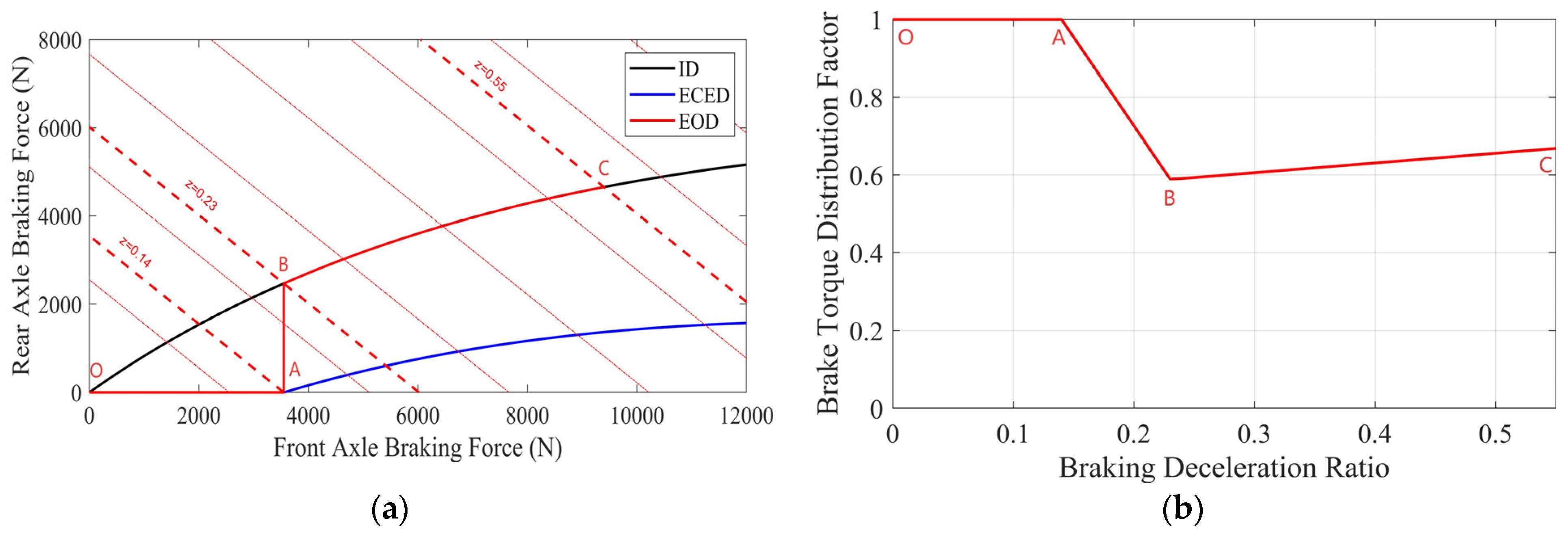
The Energy-Optimized Distribution (EOD) curve follows the OA–AB–BC construction. In the OA segment, the braking intensity is low, and all regenerative braking is assigned to the front-axle motors; point A corresponds to $z_A=0.14$. Once the front braking force reaches the ECE admissible boundary, the front-axle braking force is held constant, and the rear-axle regenerative force is increased along segment AB. Point B occurs at $z_B=0.23$; beyond this point, the distribution follows the ideal braking-force curve BC because of the I-curve stability limit. For good-road adhesion coefficients in the range 0.6–0.9, braking intensities above $z=0.55$ are treated as emergency braking. Beyond point C, regenerative braking is disabled, and the demanded braking force is supplied by the mechanical friction brakes. The resulting front-axle motor braking coefficient is therefore defined by Equation (55), and the front/rear axle torque commands are given by Equations (56) and (57). Each motor command remains subject to speed-dependent regenerative-torque capability, battery charge acceptance, and tire-adhesion limits; any unmet braking demand is supplied by friction braking. The braking-torque distribution is shown in Figure 10.

$${\beta }_f\left(z\right)=\left\{\begin{array}{ll}1,& 0\le z\le 0.14,\\ {\displaystyle \frac{0.14}{z}},& 0.14<z<0.23,\\ {\displaystyle \frac{l_r+z{h}_g}{L}},& 0.23\le z\le 0.55,\\ 0,& z>0.55.\end{array}\right.$$

(55)

$$T_{bf}={\beta }_f\left(z\right)T_b, T_{br}=\left[1-{\beta }_f\left(z\right)\right]T_b$$

(56)

$$\left|T_{\mathrm{r}\mathrm{e}\mathrm{g}}\right|\le \mathrm{m}\mathrm{i}\mathrm{n}\left\{T_{m,\mathrm{r}\mathrm{e}\mathrm{g}\mathrm{e}\mathrm{n},\mathrm{m}\mathrm{a}\mathrm{x}},T_{\mathrm{b}\mathrm{a}\mathrm{t},\mathrm{c}\mathrm{h},\mathrm{m}\mathrm{a}\mathrm{x}},T_{\mu ,\mathrm{m}\mathrm{a}\mathrm{x}}\right\}$$

(57)

4.3. Torque Distribution Algorithm

A motor-energy-only allocation is insufficient under combined longitudinal and steering conditions because tire-slip loss, yaw-moment demand, load transfer, and actuator limits alter the preferred wheel torques. The sequential quadratic programming (SQP) allocator therefore minimizes a normalized composite objective containing motor electrical input power, longitudinal and lateral tire-slip power, and a wheel-torque increment penalty. The allocation is subject to the demanded total wheel torque, the required external yaw moment, speed-dependent motor-torque limits, and the tire-friction ellipse.

$$J_m={\displaystyle {\sum }_{i=1}^4}{P}_{\mathrm{i}\mathrm{n},i}\left(T_i,n_i\right)$$

(58)

$$J_s={\displaystyle {\sum }_{i=1}^4}\left(P_{sx,i}+P_{sy,i}\right)$$

(59)

$$J_{\mathit{\Delta }T}={\displaystyle {\sum }_{i=1}^4}{\left[T_i\left(k\right)-T_i\left(k-1\right)\right]}^2$$

(60)

The wheel-torque allocation satisfies two equality constraints: the demanded total wheel torque $T_{\mathrm{r}\mathrm{e}\mathrm{q}}$ and the required external yaw moment $\Delta M_z$, as expressed in Equation (61).

$$s.t.\left\{\begin{array}{l}{T}_{req}=T_{fl}+T_{fr}+T_{rl}+T_{rr}\\ \Delta M_z={\displaystyle \frac{d\left(-T_{fl}\cdot \cos {\delta }_1+T_{fr}\cdot \cos {\delta }_2-T_{rl}+T_{rr}\right)}{2R_e}}\\ \hspace{1em}\hspace{1em}\hspace{1em}+{\displaystyle \frac{\left(T_{fl}\cdot \sin {\delta }_1+T_{fr}\cdot \sin {\delta }_2\right)\cdot l_f}{R_e}}\end{array}\right.$$

(61)

Under steering, the external yaw-moment requirement produces left–right torque differences. The motor-energy term of the objective is therefore defined by Equation (62).

$$\min J_m={\displaystyle \sum _{i=1}^4{P}_{ini}\left(T_i,n_i\right)}$$

(62)

In the equation, $P_{in}$ represents the input power fitting function of the in-wheel-motor.

Motor input power depends on motor speed, which increases with wheel slip. To account for the associated tire loss, the longitudinal tire-slip-energy term in Equation (63) is included in the allocation objective.

$$\min J_s={\displaystyle {\displaystyle \sum _i^4}{\epsilon }_{si}\cdot T_i}={\displaystyle {\displaystyle \sum _i^4}\frac{P_{sxi}}{T_{i0}}{T}_i}$$

(63)

In the equation, ${\epsilon }_s$ represents the tire slip energy coefficient, $P_{sxi}/T_{i0}={\epsilon }_{si}$. Meanwhile, to ensure smooth vehicle operation, the output torque of the in-wheel motors should vary smoothly; therefore, a torque increment objective function for the motors is established:

$$\min J_T={\displaystyle {\displaystyle \sum _{i=1}^4}\Delta T_i^2}={\displaystyle {\displaystyle \sum _{i=1}^4}{\left(T_i-T_{i0}\right)}^2}$$

(64)

In the equation, represents the output torque at the previous time step. Therefore, the overall objective function of the energy-optimization-based torque distribution control in this paper is defined as:

$$\min J={\lambda }_m{J}_m+{\lambda }_s{J}_s+{\lambda }_T{J}_T$$

(65)

${\lambda }_m$, ${\lambda }_s$, and ${\lambda }_T$ represent the weighting coefficients for motor energy, tire slip energy, and torque increment, respectively.

The constrained nonlinear allocation is solved by sequential quadratic programming. At each iteration, the Lagrangian is approximated by a quadratic subproblem; the Hessian is updated by Broyden–Fletcher–Goldfarb–Shanno (BFGS) and the step length is selected by an Armijo line search.

$$\begin{array}{c}\min f\left(x\right)\\ s.t. \left\{\begin{array}{l}{h}_u\left(x\right)=0, u=1,2\dots p\\ g_v\left(x\right)\le 0, \mathrm{v}=1,2\dots m\end{array}\right.\end{array}$$

(66)

In Equation (66), $x$ represents the torque vector of the in-wheel motors $T$, $f\left(x\right)$ denotes the overall objective function of the torque distribution control based on energy optimization $J$, $h\left(x\right)$ corresponds to the equality constraints, and $g\left(x\right)$ corresponds to the inequality constraints. T = [T_FL,T_FR,T_RL,T_RR]^T is the wheel-torque vector, J(T) is the composite objective, h(T) = 0 contains the equality constraints, and g(T) ≤ 0 contains the actuator inequalities. Because regenerative braking is handled by the EOD branch, the SQP allocator is restricted to nonnegative propulsion torques. Equations (67) and (68) specify the equality and inequality constraints.

$$\left\{\begin{array}{l}{h}_1\left(x\right)=x_1+x_2+x_3+x_4-T_{req}\\ h_2\left(x\right)={\displaystyle \frac{d\left(-x_1\cdot \cos {\delta }_1+x_2\cdot \cos {\delta }_2-x_3+x_4\right)}{2R_e}}\\ +{\displaystyle \frac{\left(x_1\cdot \sin {\delta }_1+x_2\cdot \sin {\delta }_2\right)\cdot l_f}{R_e}}-\Delta M_z\end{array}\right.$$

(67)

$$\left\{\begin{array}{l}{g}_1\left(x\right)=-x\\ g_2\left(x\right)=x-T_{\max }\end{array}\right.$$

(68)

4.4. Torque Vectoring Control Strategy

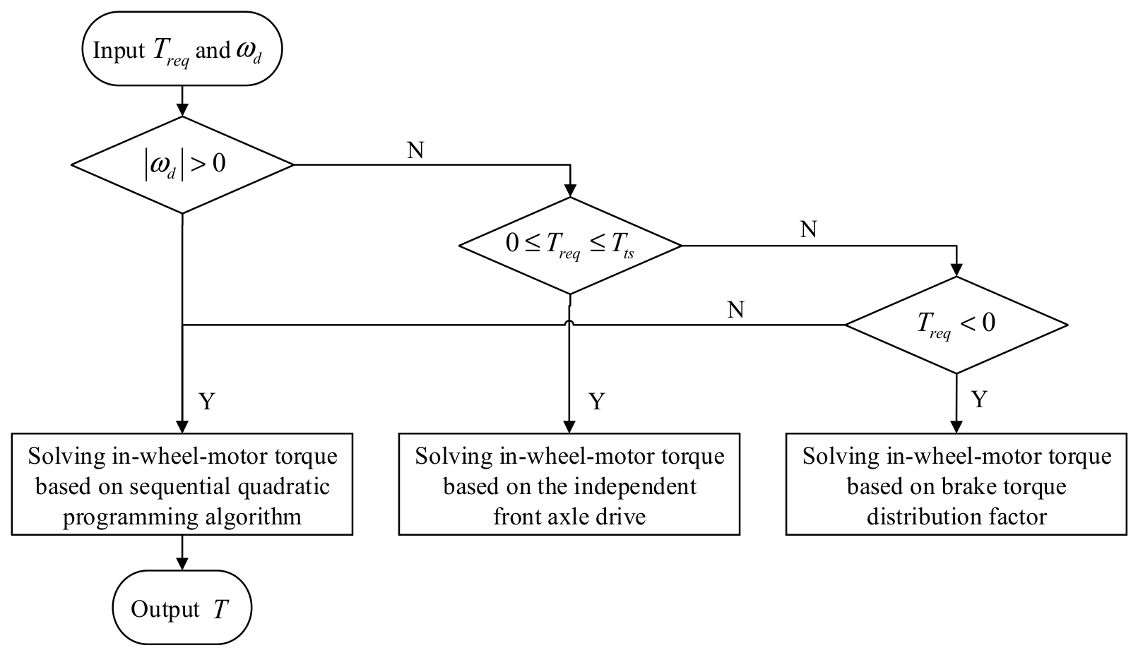
The supervisory controller contains three operating branches. Under low positive torque and approximately straight driving, front-axle-only propulsion is used when the demand is below the calibrated speed-dependent threshold and the front-tire adhesion margin is sufficient. Under general propulsion or steering, the four-wheel sequential quadratic programming allocator satisfies the total-torque and external-yaw-moment demands. As the slip ratio or tire utilization of one wheel rises, its marginal slip-energy cost increases; the optimizer consequently reduces that wheel torque and transfers the remaining demand to wheels with lower combined motor-plus-tire energy cost. During regenerative braking, the Energy-Optimized Distribution curve first determines the front–rear ratio, after which a left–right differential correction supplies the required yaw moment and a slip limiter maintains the wheel slip near the 13–17% target region. The coordinated supervisory logic is shown in Figure 11.

$$T_{\mathrm{F}\mathrm{L}}=T_{\mathrm{F}\mathrm{R}}={\displaystyle \frac{T_{\mathrm{r}\mathrm{e}\mathrm{q}}}{2}}, T_{\mathrm{R}\mathrm{L}}=T_{\mathrm{R}\mathrm{R}}=0$$

(69)

$$T_{\mathrm{F}\mathrm{L}}^0=T_{\mathrm{F}\mathrm{R}}^0={\displaystyle \frac{1}{2}}{\beta }_f\left(z\right)T_{\mathrm{r}\mathrm{e}\mathrm{q}}, T_{\mathrm{R}\mathrm{L}}^0=T_{\mathrm{R}\mathrm{R}}^0={\displaystyle \frac{1}{2}}\left[1-{\beta }_f\left(z\right)\right]T_{\mathrm{r}\mathrm{e}\mathrm{q}}$$

(70)

$$\mathit{\Delta }{T}_z={\displaystyle \frac{R_e}{d}}\mathit{\Delta }{M}_z, {\lambda }_f={\displaystyle \frac{F_{zf}}{F_{zf}+F_{zr}}}$$

(71)

$$\begin{array}{rrrr}{T}_{\mathrm{F}\mathrm{L}}& =T_{\mathrm{F}\mathrm{L}}^0-{\lambda }_f\mathit{\Delta }{T}_z,\hfill & T_{\mathrm{F}\mathrm{R}}& =T_{\mathrm{F}\mathrm{R}}^0+{\lambda }_f\mathit{\Delta }{T}_z,\hfill \\ T_{\mathrm{R}\mathrm{L}}& =T_{\mathrm{R}\mathrm{L}}^0-\left(1-{\lambda }_f\right)\mathit{\Delta }{T}_z,\hfill & T_{\mathrm{R}\mathrm{R}}& =T_{\mathrm{R}\mathrm{R}}^0+\left(1-{\lambda }_f\right)\mathit{\Delta }{T}_z\hfill \end{array}$$

(72)

$$T_{i,\mathrm{c}\mathrm{m}\mathrm{d}}=\mathrm{s}\mathrm{a}\mathrm{t}\left[T_i-K_{\kappa }\mathrm{m}\mathrm{a}\mathrm{x}\left(0,\left|{\kappa }_i\right|-{\kappa }_{\mathrm{l}\mathrm{i}\mathrm{m}}\right)\mathrm{s}\mathrm{g}\mathrm{n}\left({\kappa }_i\right)\right] {\kappa }_{\mathrm{l}\mathrm{i}\mathrm{m}}=0.15$$

(73)

When the demanded propulsion torque exceeds the lookup threshold, equal four-wheel torque is the minimizer of the reduced motor-only problem under the assumptions of Section 4.1. In the complete controller, however, tire-slip energy, yaw-moment demand, and actuator constraints are also active; therefore, the final wheel torques are obtained from the SQP allocation rather than being assumed globally optimal.

During steering, the external yaw moment generated by the active-front-steering layer requires left–right torque differences. Whenever the absolute desired yaw rate exceeds the straight-driving dead band, the four-wheel SQP allocator is activated to satisfy total-torque and yaw-moment demands while minimizing the composite energy objective.

During braking, the wheel torques are determined by the EOD front–rear coefficient under the ideal-distribution and ECE constraints. This braking branch is separate from the propulsion-mode threshold and from the positive-torque SQP problem.

$${\mathbf{T}}^{\ast }=\left\{\begin{array}{ll}{\mathbf{T}}_{\mathrm{s}\mathrm{i}\mathrm{n}\mathrm{g}\mathrm{l}\mathrm{e}\hspace{0.25em}\mathrm{a}\mathrm{x}\mathrm{l}\mathrm{e}},& T_{\mathrm{r}\mathrm{e}\mathrm{q}}>0,\hspace{0.25em}{T}_{\mathrm{r}\mathrm{e}\mathrm{q}}<T_{\mathrm{t}\mathrm{h}},\hspace{0.25em}\left|{\omega }_d\right|\le {\omega }_{\mathrm{d}\mathrm{b}},\hspace{0.25em}{\rho }_f<{\rho }_{\mathrm{l}\mathrm{i}\mathrm{m}},\\ {\mathbf{T}}_{\mathrm{S}\mathrm{Q}\mathrm{P}},& T_{\mathrm{r}\mathrm{e}\mathrm{q}}>0\hspace{0.25em}\mathrm{otherwise},\\ {\mathbf{T}}_{\mathrm{E}\mathrm{O}\mathrm{D}+\mathrm{s}\mathrm{l}\mathrm{i}\mathrm{p}},& T_{\mathrm{r}\mathrm{e}\mathrm{q}}<0\end{array}\right.$$

(74)

5. Simulation

5.1. Preparation

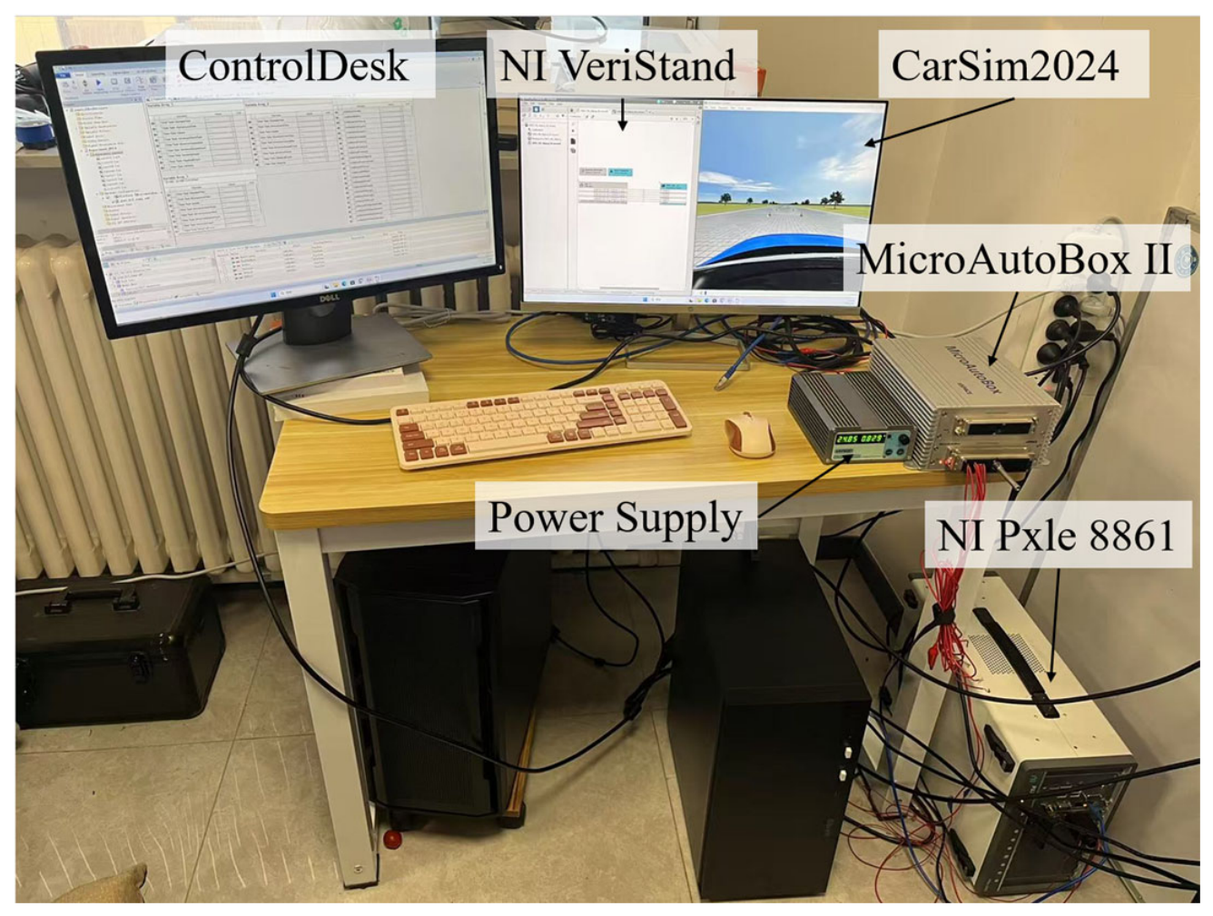
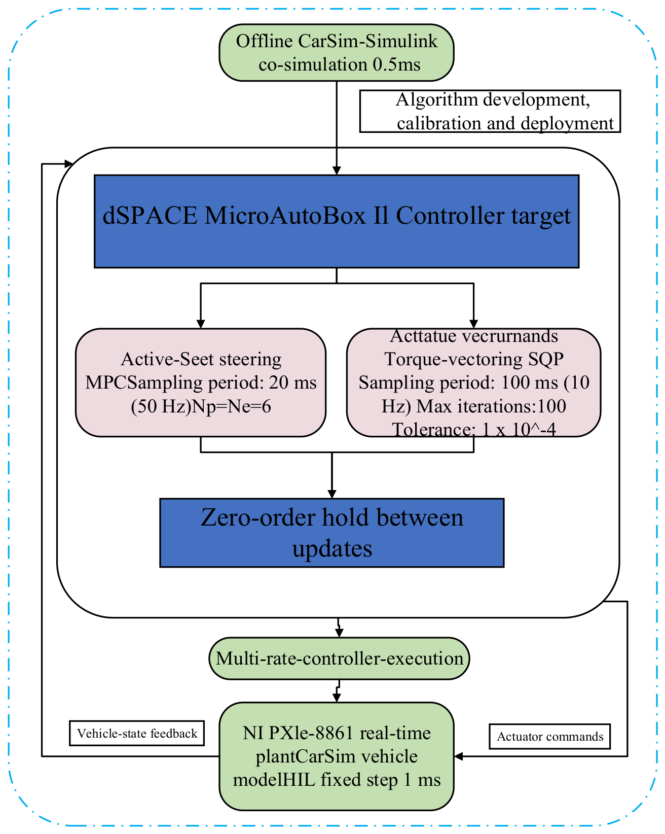
The hardware-in-the-loop (HIL) platform consists of a dSPACE MicroAutoBox II controller target, an NI PXIe-8861 real-time vehicle-model target, RTI1401 and DS1513 interface boards, and a PXIe-8512 Controller Area Network interface. The conventional offline CarSim–Simulink co-simulation uses a fixed CarSim integration step of 0.5 ms, whereas the HIL vehicle model is executed with a fixed real-time step of 1 ms. Vehicle-state feedback is transmitted from the real-time model target to the controller target, and the controller returns the front-wheel steering commands and four wheel-torque commands. ControlDesk and NI VeriStand are used for deployment, calibration, monitoring, and synchronized data acquisition. The HIL experimental platform is shown in Figure 12, and the controller, optimization, and HIL implementation settings are summarized in

Table 11. Controller, optimization, and hardware-in-the-loop implementation settings.

Item	Setting/Value	Implementation Detail
Offline CarSim integration step	0.5 ms	Fixed-step CarSim–Simulink co-simulation
HIL real-time vehicle-model step	1 ms	Fixed-step plant execution
AFS MPC sampling period	20 ms	50 Hz steering-controller update
MPC prediction horizon	6 samples	Finite prediction horizon
MPC horizon	6 samples	Finite control horizon
Torque-vectoring SQP sampling period	100 ms	10 Hz allocation update
Maximum SQP outer iterations	400	Iteration limit
SQP convergence tolerance	1 × 10−6	Termination criterion
Command intersample behavior	Zero-order hold	Most recent feasible command retained
Per-call solver timing	Not separately instrumented	Update periods are not reported as execution-time statistics

.

The active-front-steering model-predictive controller is updated every 20 ms, and the torque-vectoring sequential-quadratic-programming controller is updated every 100 ms. Both the prediction horizon and the control horizon are six samples. The SQP outer-iteration limit is 400, and the convergence tolerance is 1 × 10⁻⁶. Between consecutive controller updates, the most recent command is maintained by a zero-order hold, as expressed in Equation (75). The HIL campaign verified closed-loop operation under this multi-rate schedule. Per-call SQP execution time was not instrumented as a separate measurement channel; consequently, the manuscript reports the verified update periods and solver settings but does not equate them with measured average or worst-case execution times. Dedicated solver-timing profiling is identified as a future implementation task.

$${\mathbf{u}}_j\left(t\right)={\mathbf{u}}_j\left[k\right], k{T}_j\le t<\left(k+1\right)T_j, j\in \{\mathrm{M}\mathrm{P}\mathrm{C},\mathrm{S}\mathrm{Q}\mathrm{P}\}$$

(75)

Figure 13 summarizes the multi-rate controller implementation and bidirectional signal interaction of the HIL platform. The control algorithms are first developed, calibrated, and verified through offline CarSim–Simulink co-simulation with a fixed-step size of 0.5 ms and are subsequently deployed on the dSPACE MicroAutoBox II controller target. During HIL execution, the CarSim-based vehicle model runs on the NI PXIe-8881 real-time plant target with a fixed-step size of 1 ms. The active-front-steering MPC is updated every 20 ms, whereas the torque-vectoring SQP layer is executed every 100 ms. The plant target transmits the vehicle-state feedback required by both control algorithms—including vehicle speed, yaw rate, lateral acceleration, steering angle, and individual wheel speeds—to the controller target. The controller target calculates the commanded front-wheel steering angle and four individual wheel torques. These commands are maintained by zero-order holds between successive controller updates and returned to the real-time vehicle model as actuator commands. The communication links are identified according to their interfaces, signal types, and transmission directions, without specifying an unreported communication bit rate or cyclic-message period.

A tire-utilization-based torque-vectoring strategy (TTV) solved by quadratic programming is used as one benchmark, together with a uniform torque-vectoring strategy (UTV). The proposed strategy is denoted energy-optimized torque vectoring (ETV).

Tire workload is defined as the ratio of the resultant tire force to the available friction force under the current vertical load and road-adhesion coefficient [29]. It represents the utilized fraction of tire-force capacity:

$${\eta }_i={\displaystyle \frac{\sqrt{F_{xi}^2+F_{yi}^2}}{\mu F_{zi}}}, i\in \left\{fl,fr,rl,rr\right\}$$

(76)

In the formula, $\eta$ represents the Tire-Workload-Usage, and $\mu$ denotes the road adhesion coefficient.

The simulation conditions include the US06 urban driving cycle and the double lane-change maneuver. The Uncontrolled Torque Vectoring strategy and the Tire-Workload-Usage Torque Vectoring strategy are used as comparison strategies against the Energy-Optimization Torque Vectoring strategy proposed in this paper, as shown in

Table 12. Comparison of the control strategies.

Steering Control	Braking Torque Allocation	Propulsion Torque Allocation	Strategy
Base steering	Ideal distribution	Equal distribution	UTV
Base steering	Ideal distribution	Tire-utilization-based	TTV
AFS	EOD	Energy-optimized	ETV

.

Three strategies are compared: uniform torque vectoring (UTV), tire-utilization-based torque vectoring (TTV), and the proposed energy-optimized torque vectoring (ETV). Their propulsion, braking, and steering functions are summarized in Table 12.

5.2. Longitudinal Simulation

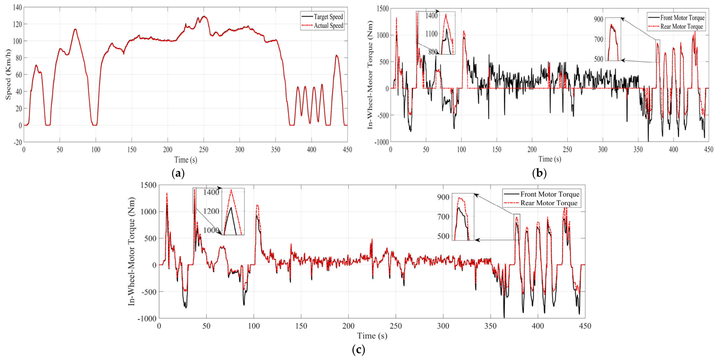
To demonstrate the combined optimization of in-wheel-motor efficiency and tire longitudinal-slip energy, the road-adhesion coefficient of the high-acceleration Supplemental Federal Test Procedure driving cycle (US06) is set to 0.5.

Figure 14b,c show the motor torques obtained with ETV and TTV, respectively. On the low-adhesion road, ETV accounts for both motor input power and longitudinal tire-slip loss. During intervals of low torque demand, the vehicle mainly operates in front-axle drive, whereas the four-wheel allocator is activated as the demand or tire constraints increase.

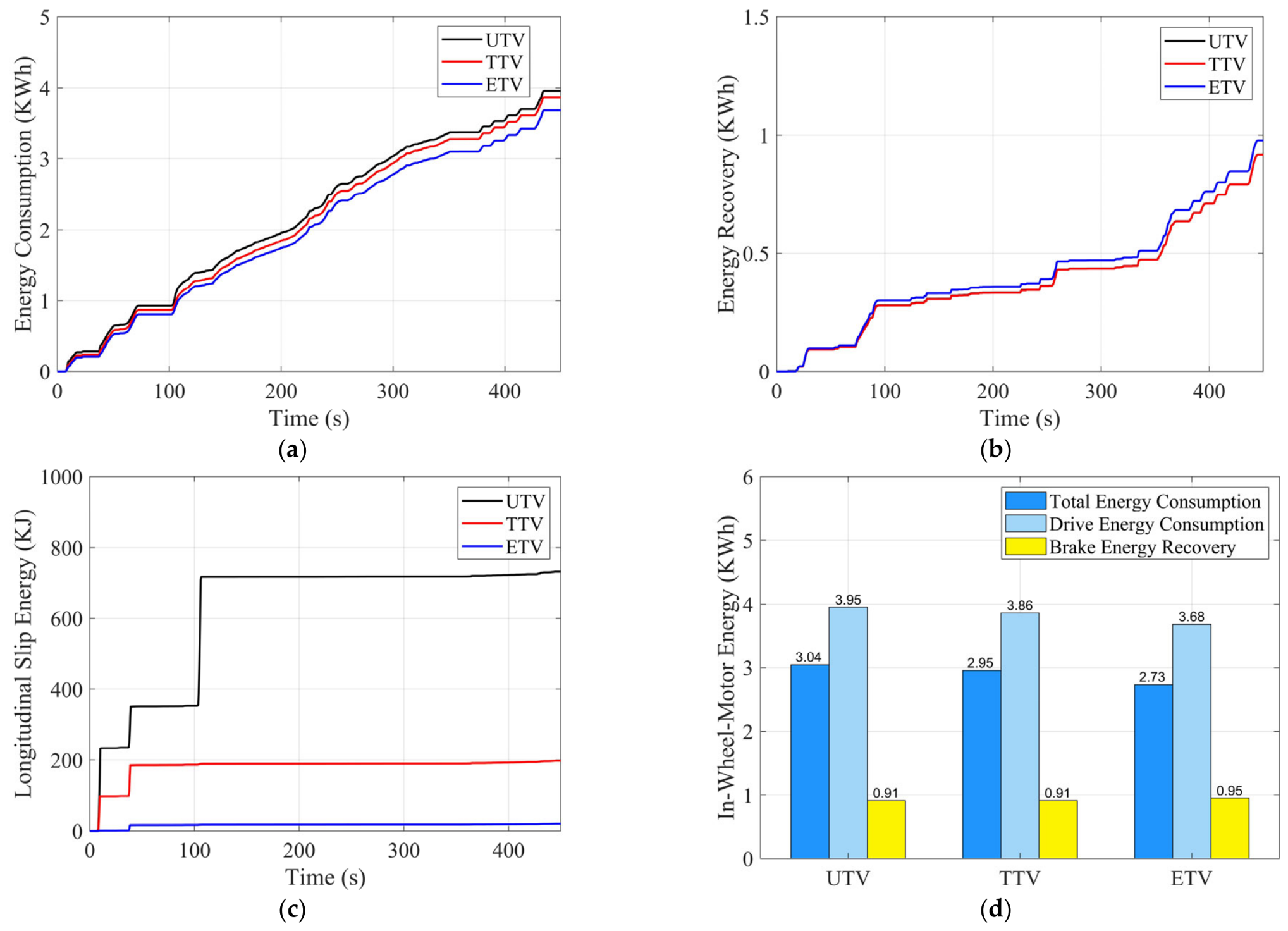
ETV consumes less driving energy than TTV and UTV. TTV also outperforms UTV because reducing tire workload decreases longitudinal slip loss, as shown in Figure 15c.

Figure 15d compares the motor-energy terms. Relative to UTV, ETV increases recovered electrical energy by 4.39% and reduces propulsion energy by 6.83%; relative to TTV, it reduces propulsion energy by 4.66%. The resulting total motor-energy reductions are 10.19% and 7.45% relative to UTV and TTV, respectively.

5.3. Steering Simulation

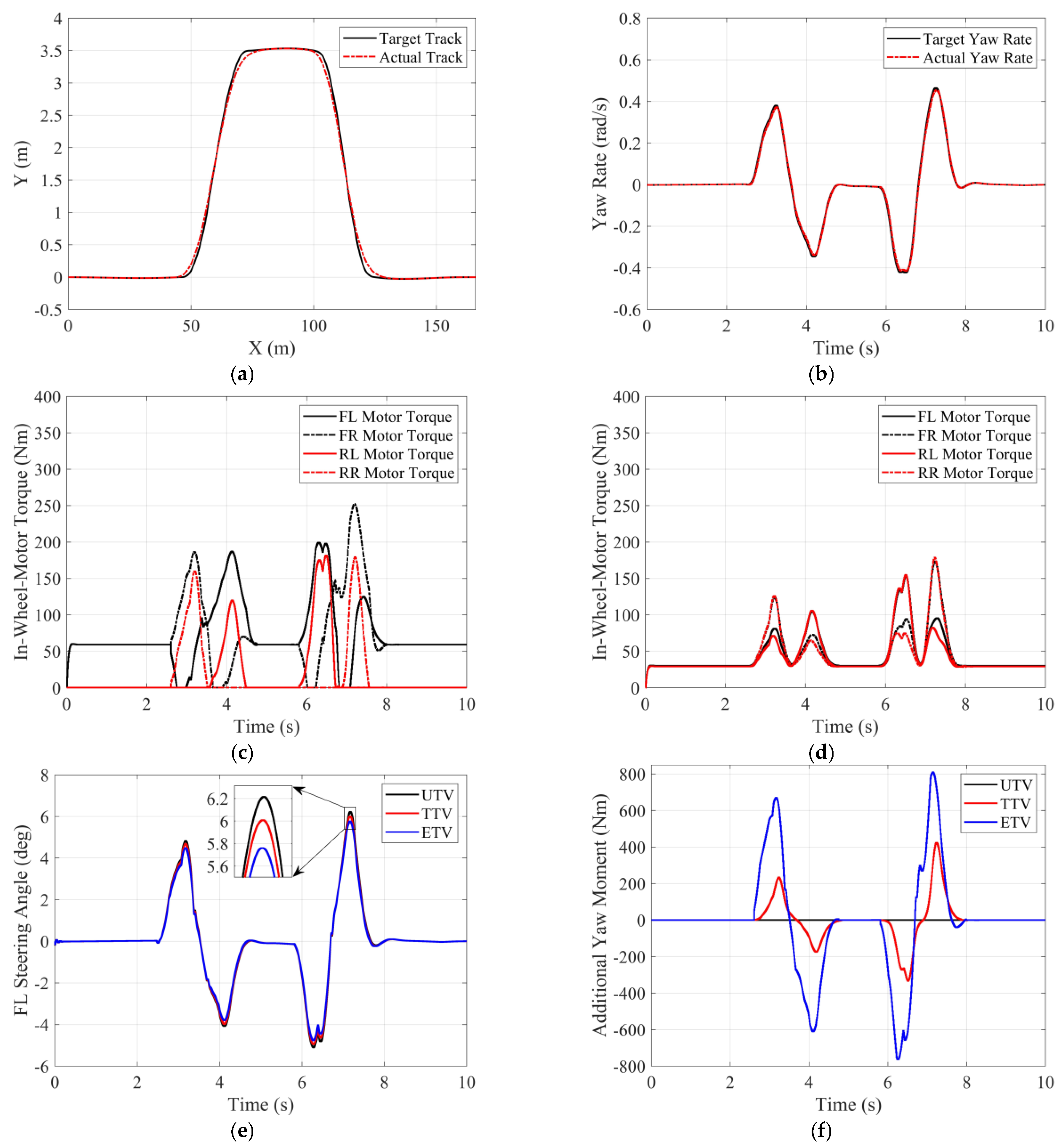
The double-lane-change maneuver is performed at a target speed of 60 km/h on a road with an adhesion coefficient of 0.8.

Figure 16a,b show that the active-front-steering controller maintains trajectory and yaw-rate tracking while reducing the front-wheel steering demand through the external yaw moment.

Figure 16c,d compare the wheel torques obtained with ETV and TTV. ETV activates the wheel motors according to the demanded longitudinal force and yaw moment, so that one rear motor may remain passive during portions of the maneuver.

As the maneuver ends, the desired yaw rate and external yaw moment decrease. The rear-axle torques then approach zero, and the front-wheel torques converge, returning the vehicle to the front-axle mode when the propulsion demand is below the calibrated threshold.

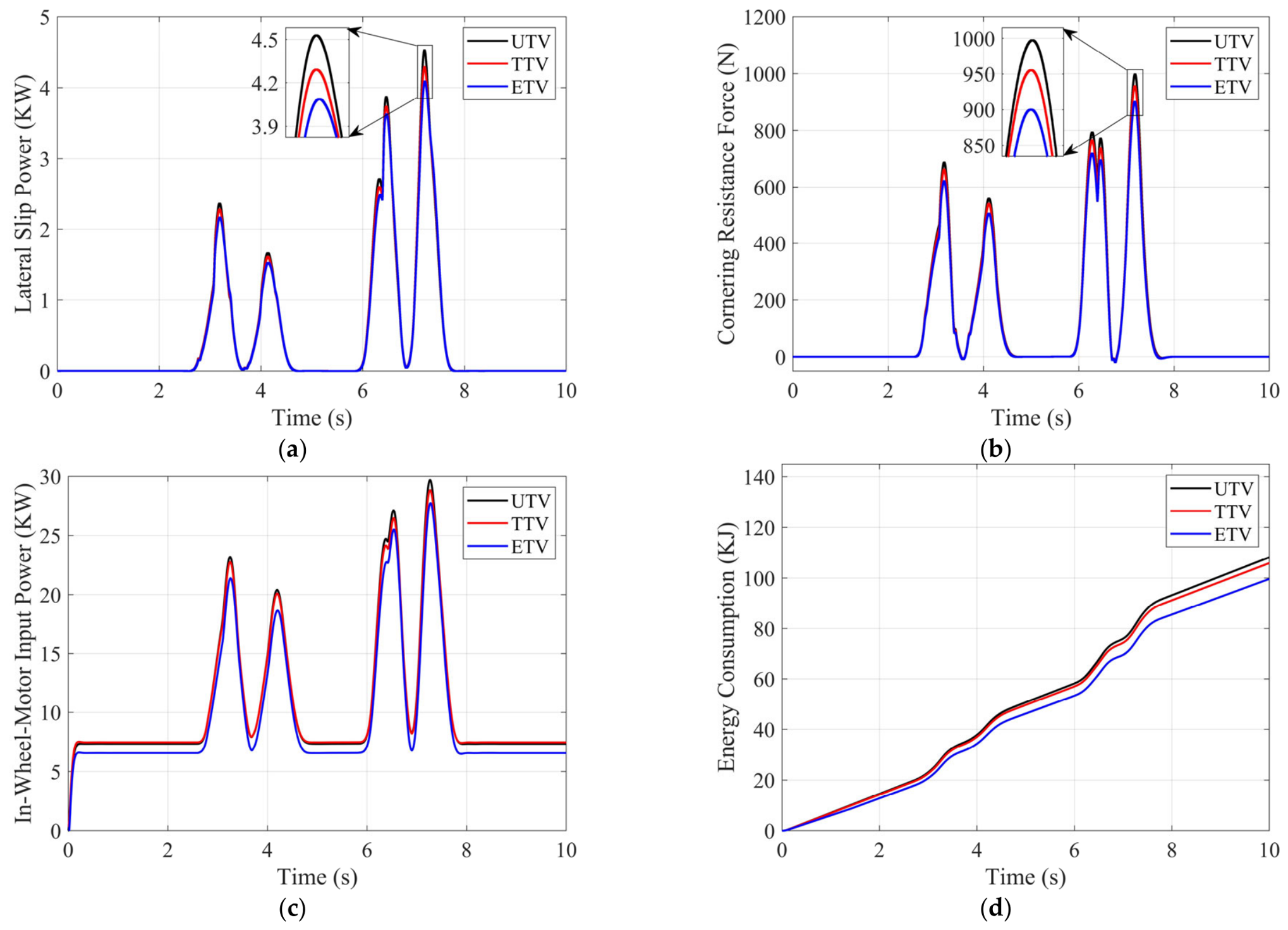
The comparison of front-wheel steering angles confirms that the active-front-steering controller reduces steering demand by coordinating the external yaw moment. Figure 17b shows the corresponding reduction in cornering resistance.

Figure 17a shows that the reduced steering angle also decreases lateral tire-slip power. The maximum reductions achieved by ETV are 6.48% relative to UTV and 3.88% relative to TTV.

The coordinated reduction in motor losses and cornering resistance also lowers in-wheel-motor input power. Because TTV produces less cornering resistance than UTV, its input power is also lower than that of UTV.

The peak in-wheel-motor input power with ETV is reduced by 6.57% and 4.53% relative to UTV and TTV, respectively. The corresponding propulsion-energy reductions are 9.26% and 7.11%.

5.4. Adaptive Design Features and Scope of Validation

The model predictive active-front-steering controller does not use a single fixed pair of input penalties over the complete operating range. The fuzzy supervisor adjusts the penalties associated with the front-wheel steering-angle increment and the external-yaw-moment increment according to vehicle speed and the absolute value of the preceding steering demand. The corresponding input domains, membership functions, output factors, and rule bases are defined in Section 3.2. This scheduling mechanism provides operating-point-dependent coordination between steering intervention and differential wheel torque over the evaluated speed and steering ranges. The robustness provisions are summarized in

Table 13. Robustness provisions and corresponding implementation and validation evidence.

Controller Element	Robustness Provision	Implementation and Validation Evidence
MPC steering/yaw-moment balance	Fuzzy scheduling of the two input penalties	Membership functions, rule bases, and double-lane-change validation
SQP multi-objective allocation	Normalization of motor-energy, tire-slip-energy, and torque-increment terms	Common physical constraints retained at every update
Propulsion-mode threshold	KKT analytical condition cross-checked by offline PSO	25 rpm threshold table and existing multi-condition simulations
Claim scope	No complete-cycle global-optimality claim	Conclusions limited to the evaluated operating conditions

.

The sequential-quadratic-programming allocator employs a weighted objective containing motor input power, tire-slip energy, and wheel-torque increments. The motor-energy term promotes operation in lower-input-power regions, the tire-slip-energy term suppresses excessive longitudinal and lateral tire slip, and the torque-increment term improves command continuity. At each SQP update, the four wheel torques remain subject to the total demanded torque, external yaw moment, motor torque limits, and tire–road friction constraints. The present study explains the physical role of the three objective terms and evaluates the resulting controller under multiple operating conditions. A separate numerical sweep of the SQP weighting coefficients was not included in the completed validation.

For the reduced propulsion-mode problem, the switching structure derived from the Karush–Kuhn–Tucker conditions is numerically cross-checked using the offline particle-swarm-optimization procedure described in Section 4.1. Both methods use the speed-dependent motor-power characteristics fitted from the calibrated motor map, but they employ different solution procedures: the analytical derivation explains the switching structure, whereas the particle-swarm search calibrates the numerical threshold at 25 rpm intervals. The calibrated threshold is stored in a one-dimensional lookup table for online implementation.

The validation includes the Worldwide Harmonized Light Vehicles Test Proce-dure cycle, low-adhesion straight-line acceleration, a constant-speed figure-eight maneuver, the United States high-acceleration driving cycle, and a double-lane-change maneuver. These cases evaluate motor operating-mode selection, regenerative-energy recovery, longitudinal tire-slip suppression, steering-resistance reduction, lateral tire-slip reduction, and real-time longitudinal–steering coordination. The validation conditions and corresponding energy mechanisms are summarized in

Table 14. Existing validation conditions and the principal energy mechanism evaluated.

Condition	Validation Platform	Principal Mechanism Evaluated
WLTP cycle, μ = 0.8	Offline Simulink simulation	Low-demand motor operating-mode selection and regenerative energy recovery
Low-adhesion straight-line acceleration	Offline Simulink simulation	Longitudinal tire-slip energy and front–rear torque redistribution
Figure-eight maneuver	Offline Simulink simulation	Steering resistance and lateral tire-slip energy
US06 cycle, μ = 0.5	Hardware-in-the-loop simulation	Combined motor and longitudinal-slip energy under a high-dynamic cycle
Double-lane-change maneuver	Hardware-in-the-loop simulation	Active steering, yaw-moment coordination, and lateral-slip energy

. The conclusions are limited to these evaluated conditions. A systematic full-controller weight-sensitivity analysis and vehicle-level nonlinear model predictive control or dynamic-programming benchmark are reserved for future work.

5.5. Validation Under Additional Operating Conditions

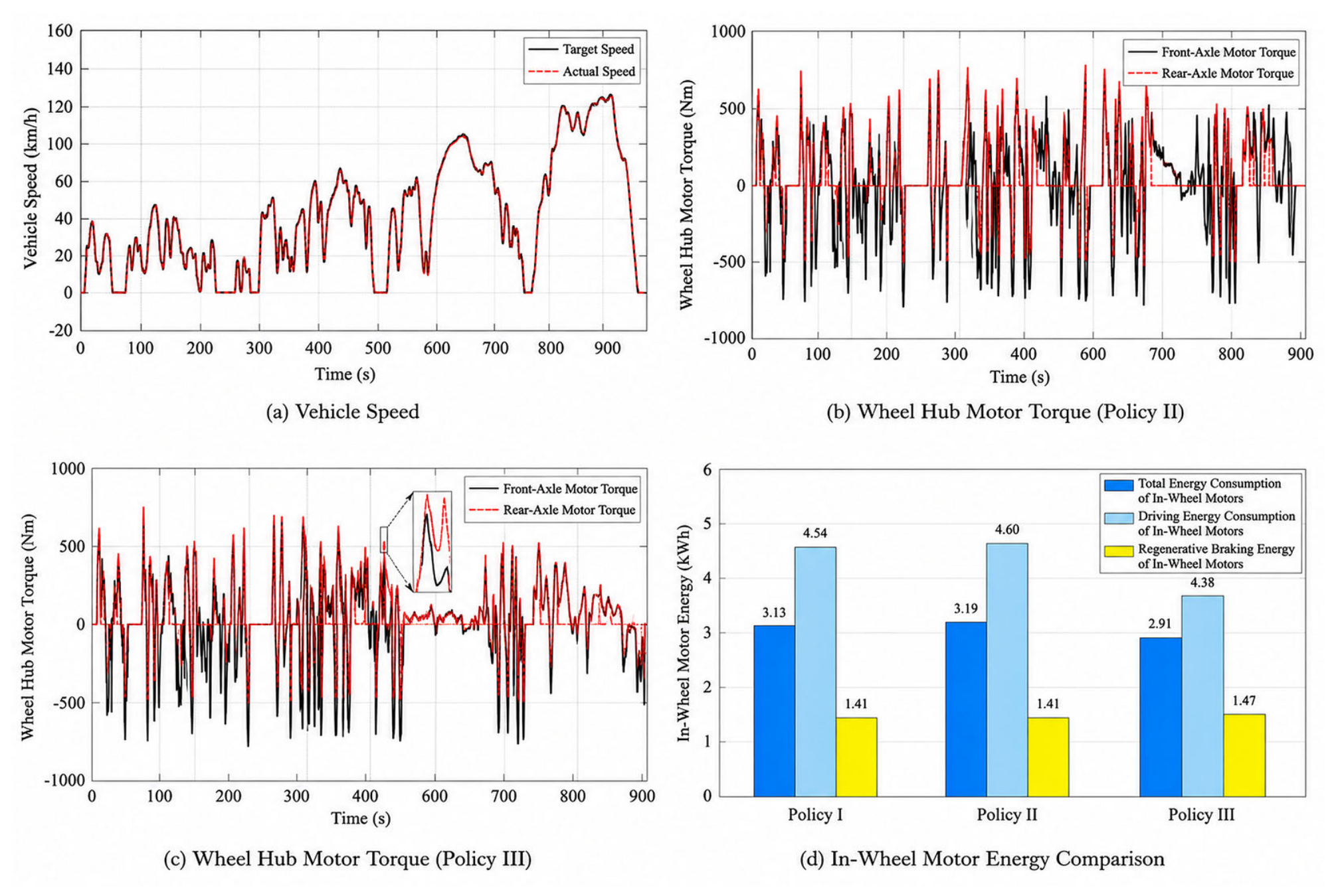
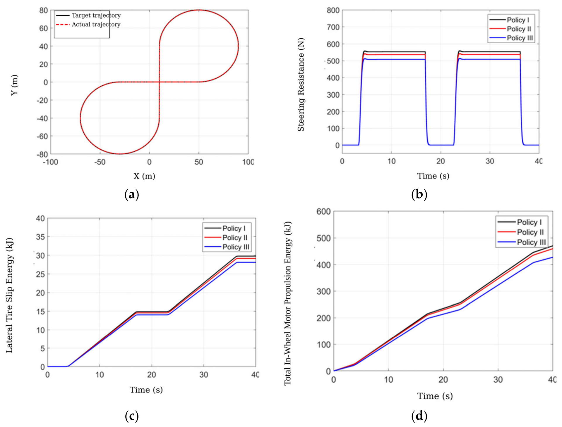
In addition to the hardware-in-the-loop tests under the US06 cycle and the double-lane-change maneuver, the completed offline validation includes a Worldwide Harmonized Light Vehicles Test Procedure cycle, low-adhesion straight-line acceleration, and a constant-speed figure-eight maneuver. Uniform torque vectoring corresponds to Policy I, tire-utilization-based torque vectoring corresponds to Policy II, and the proposed energy-optimized torque-vectoring strategy corresponds to Policy III. The WLTP, straight-line acceleration, and figure-eight results are shown in Figure 18, Figure 19, and Figure 20, respectively, and the energy-saving values are summarized in

Table 15. Energy-saving results under additional offline operating conditions.

Condition	Metric	ETV vs. UTV	ETV vs. TTV
WLTP, μ = 0.8	Total motor energy	−7.03%	−8.78%
WLTP, μ = 0.8	Driving electrical energy	−3.52%	−4.78%
WLTP, μ = 0.8	Recovered electrical energy	+4.25% (increase)	+4.25% (increase)
10–100 km/h in 6 s, μ = 0.5	Driving electrical energy	Not available for this comparison	−15.04%
10–100 km/h in 6 s, μ = 0.5	Maximum longitudinal slip power	≤5 kW for ETV	≤5 kW for ETV
Figure-eight, 50 km/h, R = 40 m, μ = 0.8	Driving electrical energy	−8.54%	−6.59%
Figure-eight, 50 km/h, R = 40 m, μ = 0.8	Lateral tire-slip energy	−5.27%	−3.36%
Figure-eight, 50 km/h, R = 40 m, μ = 0.8	Cornering resistance	−8.07%	−5.24%

.

Under the WLTP cycle with a road-friction coefficient of 0.8, the proposed strategy preferentially activates the front-axle motors when the demanded torque is low and approaches equal four-wheel torque allocation as the demanded torque increases. Relative to UTV and TTV, ETV reduces driving electrical energy by 3.52% and 4.78%, respectively, and reduces total motor energy by 7.03% and 8.78%, respectively. The recovered electrical energy is reported to increase by 4.25% relative to the two benchmark strategies.

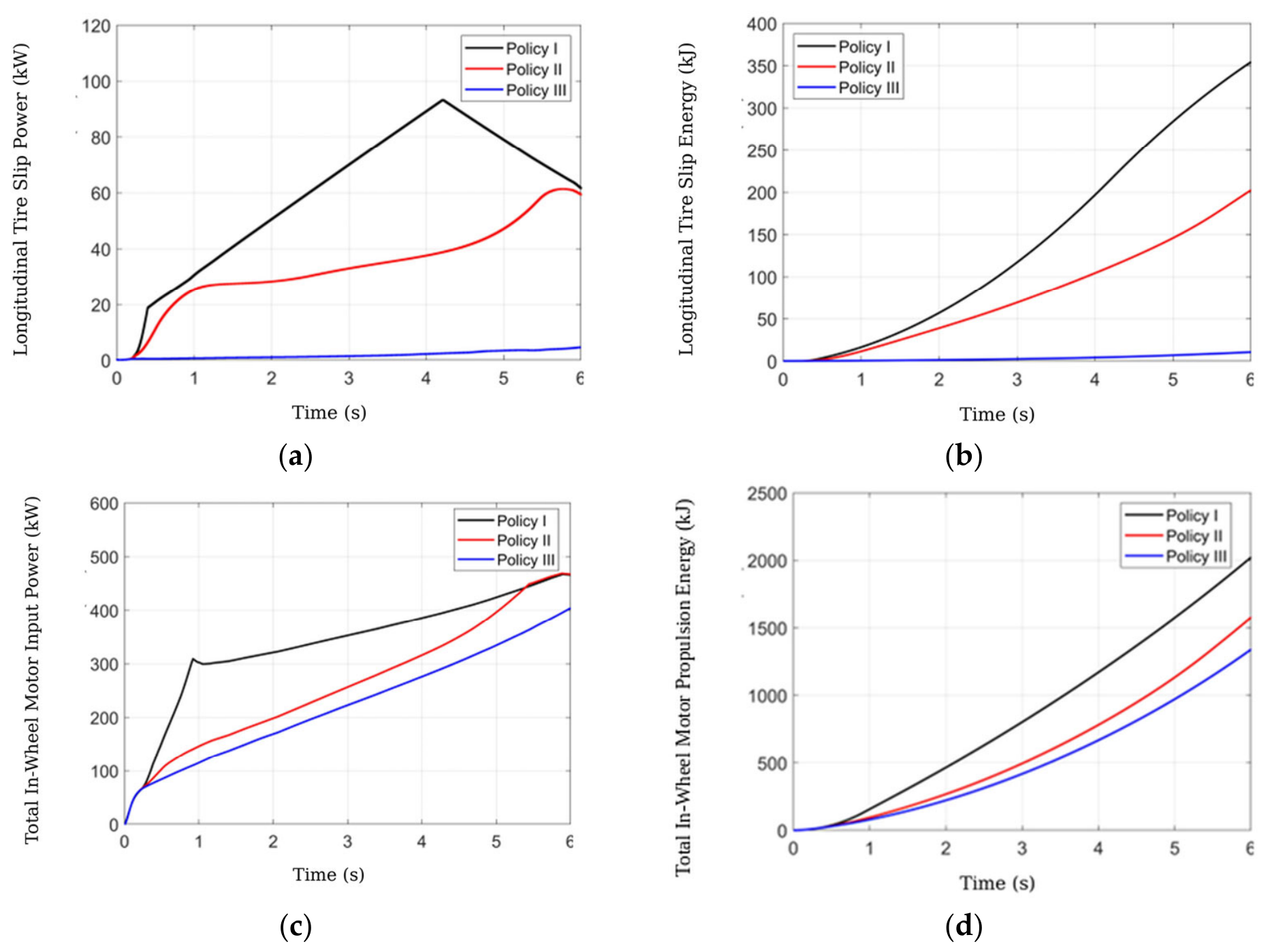
Under the low-adhesion straight-line acceleration condition, the vehicle accelerates from 10 to 100 km/h within 6 s on a road with μ = 0.5. By including longitudinal tire-slip energy in the allocation objective, ETV limits the maximum longitudinal tire-slip power to below 5 kW. The driving electrical energy is reduced by 15.04% relative to TTV. The corresponding reduction relative to UTV was not reported in the source simulation results and is therefore not inferred here.

Under the figure-eight condition at 50 km/h, with a turning radius of 40 m and μ = 0.8, ETV coordinates the front-wheel steering angles and external yaw moment while redistributing the four-wheel torques. Relative to UTV and TTV, respectively, ETV reduces driving electrical energy by 8.54% and 6.59%, lateral tire-slip energy by 5.27% and 3.36%, and cornering resistance by 8.07% and 5.24%.

6. Conclusions

This study developed a real-time energy-optimized longitudinal–steering coordinated torque-vectoring framework for a four-wheel-drive electric vehicle equipped with independently controlled in-wheel motors. The proposed strategy is denoted energy-optimized torque vectoring (ETV), while uniform torque vectoring (UTV) and tire-utilization-based torque vectoring (TTV) are used as benchmark strategies. The main conclusions are as follows:

• A model-predictive active-front-steering controller was developed to coordinate the front-wheel steering angle and external yaw moment. Fuzzy scheduling of the corresponding input penalties reduces steering resistance and lateral tire-slip energy while maintaining trajectory- and yaw-rate-tracking performance.
• For positive-torque propulsion, the Karush–Kuhn–Tucker analysis establishes the switching structure between single-axle and equal four-wheel drive under the reduced fixed-speed and symmetry assumptions. The speed-dependent torque threshold is calibrated offline using particle swarm optimization and implemented through a lookup table. Regenerative braking is allocated independently using the Energy-Optimized Distribution curve, while sequential quadratic programming provides a constrained locally optimal four-wheel torque-allocation solution for general propulsion and steering conditions.
• The offline simulations demonstrate the effectiveness of ETV under different energy-loss mechanisms. Under the WLTP cycle, ETV reduced total motor energy by 7.03% relative to UTV and by 8.78% relative to TTV. During low-adhesion straight-line acceleration, ETV reduced propulsion electrical energy by 15.04% relative to TTV and limited the maximum longitudinal tire-slip power to below 5 kW. In the figure-eight maneuver, ETV reduced propulsion electrical energy by 8.54% relative to UTV and by 6.59% relative to TTV, with corresponding reductions in lateral tire-slip energy of 5.27% and 3.36%.
• The hardware-in-the-loop results further confirm the effectiveness of the proposed framework. Under the low-adhesion US06 cycle, ETV reduced total motor energy by 10.19% relative to UTV and by 7.45% relative to TTV. In the double-lane-change test at 60 km/h and μ = 0.8, ETV reduced propulsion electrical energy by 9.26% relative to UTV and by 7.11% relative to TTV, while the maximum lateral tire-slip power decreased by 6.48% and 3.88%, respectively.

Overall, the proposed framework reduces motor electrical energy consumption and longitudinal and lateral tire-slip losses under the evaluated propulsion, regenerative-braking, and steering conditions. However, the reported results do not constitute proof of mathematical global optimality over an arbitrary complete driving cycle. Future work will focus on full-vehicle experiments, systematic controller-weight sensitivity analysis, dedicated execution-time profiling, and vehicle-level comparisons with nonlinear model predictive control and dynamic programming.

References

1. Liang, Y.; Zhao, W.; Wu, J.; Xu, K.; Zhou, X.; Luan, Z.; Wang, C. Energy-efficient driving for distributed electric vehicles considering wheel loss energy: A distributed strategy based on multi-agent architecture. Appl. Energy 2025, 384, 125462. [Google Scholar] [CrossRef] [Scilit]
2. Jin, L.; Fan, J.; Teng, F. Coordinated control strategy of electro-mechanical composite braking for four-wheel drive electric vehicles. Proc. Inst. Mech. Eng. Part D J. Automob. Eng. 2025, 239, 2838–2853. [Google Scholar]
3. Wang, C.; Heng, B.; Zhao, W. Yaw and lateral stability control for four-wheel-independent steering and four-wheel-independent driving electric vehicle. Proc. Inst. Mech. Eng. Part D J. Automob. Eng. 2020, 234, 409–422. [Google Scholar]
4. Qiu, N.; Jin, L.; Tian, D.; Teng, F.; Fan, J.; Jin, B.; Li, A. Decoupled control of handling and stability for 4WID&4WIS vehicles under extreme conditions. Veh. Syst. Dyn. 2025, 1–24. [Google Scholar] [CrossRef] [Scilit]
5. Kim, S.H.; Kim, K.-K.K. Model predictive control for energy-efficient yaw-stabilizing torque vectoring in electric vehicles with four in-wheel motors. IEEE Access 2023, 11, 37665–37680. [Google Scholar] [CrossRef] [Scilit]
6. Peng, H.; Wang, W.; Xiang, C.; Li, L.; Wang, X. Torque coordinated control of four in-wheel motor independent-drive vehicles with consideration of the safety and economy. IEEE Trans. Veh. Technol. 2019, 68, 9604–9618. [Google Scholar] [CrossRef] [Scilit]
7. Pennycott, A.; De Novellis, L.; Sabbatini, A.; Gruber, P.; Sorniotti, A. Reducing the motor power losses of a four-wheel drive, fully electric vehicle via wheel torque allocation. Proc. Inst. Mech. Eng. Part D J. Automob. Eng. 2014, 228, 830–839. [Google Scholar] [CrossRef] [Scilit]
8. Chatzikomis, C.; Zanchetta, M.; Gruber, P.; Sorniotti, A.; Modic, B.; Motaln, T.; Blagotinsek, L.; Gotovac, G. An energy-efficient torque-vectoring algorithm for electric vehicles with multiple motors. Mech. Syst. Signal Process. 2019, 128, 655–673. [Google Scholar] [CrossRef] [Scilit]
9. Parra, A.; Tavernini, D.; Gruber, P.; Sorniotti, A.; Zubizarreta, A.; Perez, J. On nonlinear model predictive control for energy-efficient torque-vectoring. IEEE Trans. Veh. Technol. 2021, 70, 173–188. [Google Scholar] [CrossRef] [Scilit]
10. Hu, J.; Li, J.; Hu, Z.; Zhang, B.; Xu, L.; Ouyang, M. Energy-efficient torque-allocation strategy for a 6 × 6 vehicle using electric wheels. eTransportation 2021, 10, 100136. [Google Scholar] [CrossRef] [Scilit]
11. Suzuki, Y.; Kano, Y.; Abe, M. A study on tyre force distribution controls for full drive-by-wire electric vehicle. Veh. Syst. Dyn. 2014, 52, 235–250. [Google Scholar] [CrossRef] [Scilit]
12. Gao, B.; Yan, Y.; Chu, H.; Chen, H.; Xu, N. Torque allocation of four-wheel drive EVs considering tire slip energy. Sci. China Inf. Sci. 2022, 65, 122202. [Google Scholar]
13. Zhao, B.; Xu, N.; Chen, H.; Guo, K.; Huang, Y. Design and experimental evaluations on energy-efficient control for 4WIMD-EVs considering tire slip energy. IEEE Trans. Veh. Technol. 2020, 69, 14631–14644. [Google Scholar] [CrossRef] [Scilit]
14. Kobayashi, T.; Katsuyama, E.; Sugiura, H.; Ono, E.; Yamamoto, M. Efficient direct yaw moment control: Tyre slip power loss minimisation for four-independent wheel drive vehicle. Veh. Syst. Dyn. 2018, 56, 719–733. [Google Scholar]
15. Najjari, B.; Mirzaei, M.; Tahouni, A. Decentralized integration of constrained active steering and torque vectoring systems to energy-efficient stability control of electric vehicles. J. Frankl. Inst. 2022, 359, 8713–8741. [Google Scholar] [CrossRef] [Scilit]
16. Choi, J.H.; Kim, D.; Eo, J.S.; Oh, S. Energy-saving algorithm considering cornering resistance of a four-wheel independent drive electric vehicle with vehicle-to-vehicle (V2V) information. IEEE Access 2022, 10, 104398–104407. [Google Scholar] [CrossRef] [Scilit]
17. Wang, J.; Gao, S.; Wang, K.; Wang, Y.; Wang, Q. Wheel torque distribution optimization of four-wheel independent-drive electric vehicle for energy-efficient driving. Control Eng. Pract. 2021, 110, 104779. [Google Scholar] [CrossRef] [Scilit]
18. Liu, S.; Zhang, H.; Wang, S.; Zhao, X. Hierarchical torque vectoring control strategy of distributed driving electric vehicles considering handling stability and energy consumption. Sensors 2025, 25, 3933. [Google Scholar] [CrossRef] [Scilit] [PubMed]
19. Janardhanan, S.; Persson, J.; Jonasson, M.; Jacobson, B.; Gelso, E.R.; Henderson, L. Energy-efficient wheel torque distribution for heavy electric vehicles with adaptive model predictive control and control allocation. IEEE Open J. Veh. Technol. 2025, 6, 2909–2924. [Google Scholar] [CrossRef] [Scilit]
20. Chen, H.; Du, P.; Wang, Y.; Jin, D.; Lian, X. Dynamic energy-efficient torque allocation algorithm for in-wheel motor-driven vehicle. Proc. Inst. Mech. Eng. Part D J. Automob. Eng. 2020, 234, 1815–1825. [Google Scholar] [CrossRef] [Scilit]
21. Zhao, B.; Xu, N.; Chen, H.; Guo, K.; Huang, Y. Stability control of electric vehicles with in-wheel motors by considering tire slip energy. Mech. Syst. Signal Process. 2019, 118, 340–359. [Google Scholar] [CrossRef] [Scilit]
22. Guo, K.; Zhuang, Y.; Lu, D.; Chen, S.-K.; Lin, W. A study on speed-dependent tyre–road friction and its effect on the force and the moment. Veh. Syst. Dyn. 2005, 43, 329–340. [Google Scholar] [CrossRef] [Scilit]
23. Morera-Torres, E.; Ocampo-Martinez, C.; Bianchi, F.D. Experimental modelling and optimal torque vectoring control for 4WD vehicles. IEEE Trans. Veh. Technol. 2022, 71, 4922–4932. [Google Scholar] [CrossRef] [Scilit]
24. Zhang, H.; Zhang, Y.; Liu, C.; Zhang, Z. Energy efficient path planning for autonomous ground vehicles with ackermann steering. Rob. Auton. Syst. 2023, 162, 104366. [Google Scholar] [CrossRef] [Scilit]
25. Ikezawa, Y.; Fujimoto, H.; Kawano, D.; Goto, Y.; Takeda, Y.; Sato, K. Range Extension Autonomous Driving for electric vehicle based on optimal vehicle velocity profile in consideration of cornering. Electr. Eng. Jpn. 2019, 207, 43–54. [Google Scholar]
26. Sun, W.; Rong, J.; Wang, J.; Zhang, W.; Zhou, Z. Research on optimal torque control of turning energy consumption for EVs with motorized wheels. Energies 2021, 14, 6947. [Google Scholar] [CrossRef] [Scilit]
27. Lenzo, B.; De Filippis, G.; Dizqah, A.M.; Sorniotti, A.; Gruber, P.; Fallah, S.; De Nijs, W. Torque distribution strategies for energy-efficient electric vehicles with multiple drivetrains. J. Dyn. Syst. Meas. Control 2017, 139, 121004. [Google Scholar] [CrossRef] [Scilit]
28. Xu, S.; Li, J.; Zhang, X.; Song, J.; Zeng, X. Research on composite braking control strategy of four-wheel-drive electric vehicles with multiple motors based on braking energy recovery optimization. IEEE Access 2023, 11, 110151–110163. [Google Scholar] [CrossRef] [Scilit]
29. Zhang, C.; Zhang, R.; Wang, R.; Chang, B.; Ma, J. Design of torque distribution strategy for four-wheel-independent-drive electric vehicle. Autom. Control Comput. Sci. 2020, 54, 501–512. [Google Scholar] [CrossRef] [Scilit]
Figure 1. Overall Architecture of the Torque Vectoring Control Strategy.
Actuators 15 00392 g001
Figure 2. Vehicle trajectory prediction under the assumption of a constant yaw rate.
Actuators 15 00392 g002
Figure 3. Efficiency map of the in-wheel motor.
Actuators 15 00392 g003
Figure 4. Deformation of the bristles within the tire contact patch.
Actuators 15 00392 g004
Figure 5. Tire forces and slip power: (a) longitudinal force and longitudinal slip force; (b) longit-dinal slip power; (c) lateral force and lateral slip force; and (d) lateral slip power.
Actuators 15 00392 g005
Figure 6. Cornering resistance force.
Actuators 15 00392 g006
Figure 7. Fuzzy-controller definitions: (a) vehicle-speed membership functions; (b) front-wheel steering-angle membership functions; (c) front-wheel steering-angle weight membership functions; and (d) additional yaw-moment weight membership functions; (e) Rule base for the front-wheel steering-angle weight; (f) Rule base for the additional yaw-moment weight.
Actuators 15 00392 g007
Figure 8. In-wheel-motor input power.
Actuators 15 00392 g008
Figure 9. In-wheel-motor torque threshold.
Actuators 15 00392 g009
Figure 10. Braking-torque distribution: (a) front–rear braking-force distribution; and (b) front-axle motor braking-torque distribution coefficient.
Actuators 15 00392 g010
Figure 11. Coordinated torque-vectoring supervisory logic.
Actuators 15 00392 g011
Figure 12. Hardware-in-the-loop experimental platform.
Actuators 15 00392 g012
Figure 13. Multi-rate HIL execution architecture and bidirectional signal interaction between the plant and controller targets.
Actuators 15 00392 g013
Figure 14. US06 vehicle speed and in-wheel-motor torque: (a) vehicle speed; (b) ETV motor torque; and (c) TTV motor torque.
Actuators 15 00392 g014
Figure 15. Comparison of US06 energy consumption: (a) driving energy; (b) recovered energy; (c) longitudinal slip energy; and (d) in-wheel-motor energy.
Actuators 15 00392 g015
Figure 16. Double-lane-change condition and actuator outputs: (a) trajectory; (b) yaw-rate tracking; (c) ETV motor torque; (d) TTV motor torque; (e) left-front steering angle; and (f) external yaw moment.
Actuators 15 00392 g016
Figure 17. Comparison of double-lane-change energy consumption: (a) lateral slip power; (b) cornering resistance force; (c) in-wheel-motor input power; and (d) energy consumption.
Actuators 15 00392 g017
Figure 18. WLTP simulation results: (a) vehicle speed; (b) in-wheel-motor torque under Policy II; (c) in-wheel-motor torque under Policy III; and (d) comparison of in-wheel-motor propulsion energy.
Actuators 15 00392 g018
Figure 19. Straight-line acceleration results: (a) tire longitudinal-slip power; (b) tire longitudinal-slip energy; (c) in-wheel-motor input power; and (d) in-wheel-motor propulsion energy.
Actuators 15 00392 g019
Figure 20. Figure-eight maneuver results: (a) trajectory; (b) steering resistance; (c) tire lateral-slip energy; and (d) in-wheel-motor propulsion energy.
Actuators 15 00392 g020