Terrain-Adaptive Global Path Planning Method Based on Bidirectional Variable Neighborhood Search A*

Abstract

To address the issues of low efficiency and non-smooth paths of the A* algorithm in large-scale environments, a terrain-adaptive global path planning method based on Bidirectional Variable Neighborhood Search A* (Terrain-Adaptive Bidirectional Variable Neighborhood Search A*, TA-BVNS-A*) is proposed. Based on the Digital Elevation Model (DEM), the slope resistance and obstacle repulsive potential field are calculated to guide the path to circumvent high-risk areas. Bidirectional alternating search, exponential weighting, and variable neighborhood mechanisms are introduced into the heuristic search to prevent blind expansion. Furthermore, a “node filtering + Bezier smoothing constraint” strategy is employed for post-processing optimization. Multi-scale terrain simulations demonstrate that, after smoothing, the maximum front-wheel steering angle is reduced by over 60% on average, specifically reaching 65.16% in the 100 m × 100 m large-scale map, satisfying vehicle kinematic constraints. This method significantly reduces the number of search nodes, eliminates jagged polylines and redundant nodes, and outputs an efficient and smooth global path that conforms to kinematic constraints.

1. Introduction

In recent years, with the rapid development of autonomous driving technology and artificial intelligence, the application boundaries of intelligent vehicles are undergoing a profound expansion from flat, regular structured urban roads to extremely complex and unknown unstructured off-road environments. In numerous special task scenarios such as emergency rescue, field geological exploration, and modern agricultural operations, off-road intelligent vehicles play an irreplaceable key role [1,2,3]. However, distinct from structured environments with clear lane lines, flat road surfaces, and comprehensive traffic rules, real unstructured off-road environments exhibit extremely high three-dimensional (3D) spatial complexity and unpredictability. Such environments are typically accompanied by drastic terrain elevation fluctuations, variable surface materials with diverse physical properties (e.g., hard dirt roads, soft sand, and muddy depressions), and highly irregularly distributed natural rigid obstacles (e.g., boulders, tree trunks, and ravines). In such extreme scenarios, autonomous vehicle navigation is no longer merely a geometric problem of avoiding two-dimensional (2D) planar collision boundaries, but has evolved into a systematic engineering problem profoundly constrained by multiple physical boundaries [4,5]. As the core hub of the intelligent vehicle navigation and control system, the primary task of global path planning is to plan a globally optimal, safe, and feasible reference path from the starting point to the destination within a known environmental map [6]. In off-road terrains, if the global planning algorithm lacks accurate perception and adaptive evaluation of 3D terrain features, the generated path can easily misguide the vehicle into steep slopes or high-damping dangerous areas. This not only leads to power system overloads and rapid energy consumption, but may also trigger catastrophic accidents such as severe wheel slippage, chassis bottoming out, or even vehicle rollover. Therefore, overcoming the challenges of environmental perception and modeling posed by unstructured terrains to efficiently plan a smooth path that combines absolute safety, strong terrain adaptability, and compliance with vehicle kinematics for off-road intelligent vehicles has become one of the most significant and urgent challenges in the current autonomous driving field. As a fundamental issue in the navigation of robots and intelligent vehicles, global path planning has attracted considerable attention from scholars in recent years, leading to the emergence of numerous heuristic and meta-heuristic algorithms. For instance, the genetic algorithm (GA) [7] is widely used due to its strong parallel processing and global search capabilities, but it is prone to premature convergence and falling into local optima. The simulated annealing (SA) algorithm [8] is easier to implement than GA, but faces challenges of slow convergence speed and high computational demands. The ant colony optimization (ACO) algorithm [9] offers the advantages of strong robustness and easy integration with other algorithms, but similarly suffers from slow convergence and susceptibility to local optima. Although the particle swarm optimization (PSO) algorithm [10] involves a small population and simple calculations, it has lower convergence accuracy and is prone to search stagnation. In contrast, traditional map search algorithms, such as Dijkstra’s algorithm [11], have an extremely high success rate in obtaining the shortest path; however, in large-scale environmental maps, the number of traversed nodes expands exponentially, occupying extensive memory space and severely degrading computational efficiency. To address this issue, the A* algorithm introduces a heuristic function based on Dijkstra’s algorithm, determining the expansion direction by comprehensively evaluating node costs. Due to its simple principles, easy implementation, and combination of high search efficiency with global optimality, the A* algorithm has become one of the most widely applied path planning frameworks today [12]. Nevertheless, when confronting large-scale complex maps, the A* algorithm still exposes obvious defects, such as prolonged computation times, excessively large path turning angles, and insufficient smoothness. To make the A* algorithm competent for more complex off-road navigation tasks, existing studies have improved it from multiple dimensions. Domestic and international scholars have conducted extensive research on its expansion and enhancement. Regarding the improvement of path planning efficiency, most studies focus on optimizing search strategies and refining heuristic functions. For example, some scholars introduced the Jump Point Search (JPS) strategy [13] to reduce unnecessary node evaluations, or employed a variable step-size A* algorithm [14] to dynamically adjust the search step based on obstacle distribution density. Additionally, some studies weighted the heuristic function by fusing Manhattan and Euclidean distances, or introduced parent node information to dynamically optimize the heuristic term. However, these efficiency enhancement strategies are mostly confined to 2D planar assumptions, and their heuristic functions still overly rely on pure geometric distances. When facing large-scale and highly undulating 3D off-road environments, purely distance-based heuristics often fail to reflect the actual physical traversal costs, easily leading to algorithm degradation in complex elevation terrains and triggering blind search. Regarding environmental modeling and safety evaluation, traditional improvements often remain at the level of simple dilation processing for 2D obstacles to set safety margins [15,16]. Although some recent studies have attempted to incorporate 3D terrain features into planning, their cost models are generally overly simplistic (e.g., only considering maximum off-road gradeability limits). They fail to systematically integrate continuous elevation fluctuation resistance, complex surface traversal costs, and local potential fields for preventing rigid collisions, leaving the generated paths with a high risk of bottoming out or rollover at the actual physical level. In terms of path smoothing and underlying kinematic adaptation, researchers have proposed various post-processing methods to eliminate the jagged polylines inherent in grid maps. For example, methods include changing the connecting lines from search nodes to grids to reduce the number of turns, or traversing the initial path and deleting collinear nodes to shorten the path length. Furthermore, polar polynomial curves [17], Reeds-Shepp curves, and various spline curves are widely used for smooth fitting of key nodes. However, directly applying global curve fitting to dense original grid nodes with these existing smoothing methods not only introduces a massive computational burden but also leads to over-fitted minor steering oscillations. Moreover, curve smoothing relying purely on mathematical and geometric principles often lacks secondary safety verification for the smoothed path, thus deviating from the originally safe passage corridor and intruding into high-cost, dangerous off-road areas. Aiming at the numerous shortcomings exposed by the aforementioned existing methods in complex off-road scenarios, this paper proposes a terrain-adaptive global path planning method based on bidirectional variable neighborhood search A* (Terrain-Adaptive Bidirectional Variable Neighborhood Search A*, abbreviated as TA-BVNS-A*), and combines node filtering with Bezier curves to achieve path smoothing that satisfies vehicle kinematic constraints. This research is dedicated to breaking the inherent contradiction between algorithm search efficiency and environmental adaptability/safety in large-scale unstructured environments, providing high-quality reference paths for underlying controllers. The main innovations and academic contributions of this paper can be summarized in the following three aspects: (1) A comprehensive terrain cost evaluation system for off-road environments is constructed [18]. Based on the digital elevation model (DEM) [19], this study deeply integrates the 3D local terrain slope, multi-category surface rolling resistance coefficients, rigid obstacles, and a comprehensive repulsive potential field of undulating terrain representing the hazard level of obstacles. This system breaks the evaluation standard of a single geometric distance, enabling the algorithm to actively and accurately guide the path to avoid high-risk steep areas and rigid obstacles, thereby enhancing the safety of off-road driving. (2) The TA-BVNS-A* algorithm is proposed. Based on the bidirectional alternating search A* framework [20], this paper introduces a forward-backward dynamic mutual guidance mechanism, an exponential weighting mechanism, and a variable neighborhood search mechanism [21]. By adaptively and dynamically adjusting the weight of the heuristic function, this strategy suppresses the algorithm’s blind node expansion, enabling rapid optimization calculations even in large-scale, highly complex off-road maps; (3) A combined “filter-first, smooth-later” strategy satisfying vehicle kinematic constraints is designed. This method eliminates redundant intermediate nodes and introduces third-order Bezier curves [22,23] for tangential continuous fitting, eliminating the jagged polylines of the original path. Under the premise of ensuring obstacle avoidance safety, this strategy also satisfies the maximum front-wheel steering angle limit of off-road vehicles, significantly improving vehicle ride smoothness.

Targeting the critical application background of intelligent vehicles navigating in complex unstructured off-road environments (e.g., emergency rescue, geological exploration, and agricultural operations), the remainder of this paper is organized as follows: Section 2 establishes the multi-dimensional off-road environment cost model. Section 3 details the design of the terrain-adaptive evaluation function. Section 4 introduces the path planning process based on bidirectional variable neighborhood search. Section 5 presents the path smoothing strategy. Section 6 provides the integrated system framework. Section 7 discusses the simulation results. Finally, Section 8 concludes the paper.

2. Off-Road Environment Modeling

To enable intelligent vehicles to navigate safely through complex unstructured terrains, it is fundamental to construct an accurate and comprehensive environment cost model before initiating the path search algorithm. This section details the multi-dimensional terrain evaluation system designed in this study, which forms the numerical foundation for subsequent evaluation and optimization.

There are fundamental differences between off-road environments and structured roads. The variable terrain undulations and complex surface types directly affect vehicle passability; therefore, the environment must be accurately modeled prior to path planning. First, terrain slope determines vehicle passability. An excessive slope makes passage impossible, while a smaller slope still increases driving resistance. It is necessary to extract elevation values to calculate the elevation differences across various regions, and subsequently calculate the slope resistance. Second, different surface types, such as hard dirt roads, gravel, and mud, have varying rolling resistance coefficients, which directly impact energy consumption and feasibility during passage. The passage cost must be set according to the surface type. Furthermore, continuous undulating terrain reduces ride smoothness even if the slope meets the requirements. An evaluation index for terrain undulation needs to be introduced so that the path actively avoids highly undulating areas. In summary, off-road environment modeling must comprehensively consider slope, surface type, and undulation degree to construct a cost model that accurately reflects the difficulty of passage, thereby providing precise environmental information for the improved algorithm in this paper.

2.1. DEM Construction

To accurately describe the three-dimensional terrain features of the off-road environment, this paper adopts a DEM to model the environment. The construction method of the DEM is as follows: the planning area is divided into grid cells of equal size, and each cell records the altitude of its corresponding position, namely the elevation value. Through this process, the continuous complex terrain surface is discretized into a two-dimensional elevation matrix. Each element in the matrix represents the elevation information of the corresponding grid cell, providing basic data support for subsequent terrain feature analysis. As shown in Figure 1, the continuous terrain surface is converted through rasterization into a two-dimensional matrix composed of grid cells with elevation values. Assuming the planning area is divided into M × N grid cells, the DEM can be expressed as:

$$H=\left[\begin{array}{ccc}{h}_{\mathrm{1,1}}& \dots & h_{1,N}\\ ⋮& \ddots & ⋮\\ h_{M,1}& \dots & h_{M,N}\end{array}\right],$$

(1)

where ${\mathit{h}}_{\mathit{i},\mathit{j}}$ represents the elevation value of the grid cell in the i-th row and j-th column.

The DEM grid maps are constructed with a spatial resolution of 1 m/grid. The obstacles are generated based on deterministic geometric zoning. Specifically, impassable zones (e.g., lakes) are defined by an elevation threshold where Z < 0.2 m, while additional obstacles are distributed using specific rectangular region masking (e.g., indices) as defined in the environment initialization module.

2.2. Surface Feature Analysis

2.2.1. Gradient Resistance Calculation

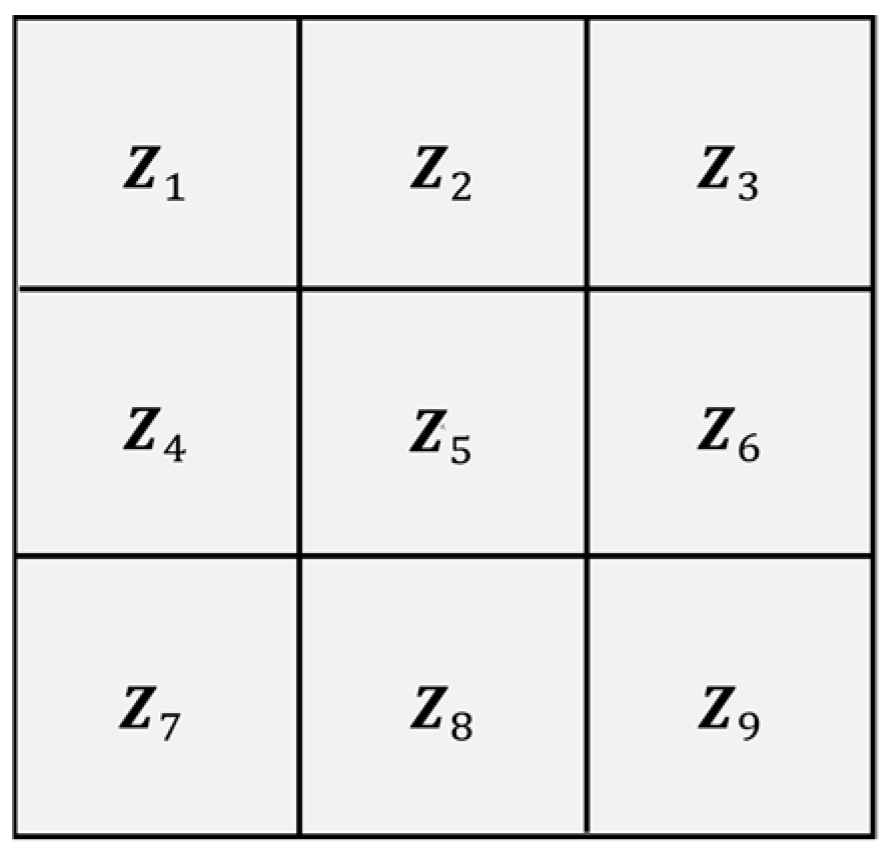
Based on the DEM data, this paper employs a 3 × 3 moving window method to calculate the surface slope to evaluate the impact of terrain undulations on vehicle traversability. As shown in Figure 2, centered on the grid cell to be calculated, the elevation values of its 8 neighboring cells are extracted to calculate the elevation change rates in the east–west and north–south directions, respectively. The calculation formulas for the elevation change rates in the east–west $f_x$ and north–south directions $f_y$ are as follows:

$$f_x=(Z_1+Z_2{ + Z}_3-Z_7-Z_8-Z_9)/6g,$$

(2)

$$f_y=(Z_3+Z_6{+Z}_9-Z_1-Z_4-Z_7)/6g,$$

(3)

where $g$ is the side length of the grid cell, and $Z_i$ is the elevation value of the corresponding grid cell.

Based on the aforementioned elevation change rates, the average slope angle $\theta$ of the center grid cell can be calculated:

$$\theta =arc\mathit{tan}\sqrt{\left(f_x^2+f_y^2\right)},$$

(4)

the defining equation of the average slope angle is used in subsequent calculations to convert two-dimensional distances into three-dimensional distances. In practical engineering applications, slope is typically expressed as a percentage, namely:

$$S=\sqrt{\left(f_x^2+f_y^2\right)}\times 100\%,$$

(5)

the maximum gradeability of typical off-road vehicles ranges from 30% to 60%. Considering both passage safety and algorithm search efficiency, this paper sets the slope constraint threshold; that is, when the slope of a grid cell exceeds 40% [18], it is considered an impassable area and assigned an infinite passage cost.

Based on the measured elevation values above, the elevation difference between the center grid cell and its adjacent grid cells can be calculated as $∆h$=${ Z}_5-Z_n$, defining the slope cost $P_{slope}$:

$$P_{slope}=k_0\cdot ∆h,$$

(6)

where $k_0$ is the slope penalty coefficient, which is assigned according to the off-road surface conditions. The reference values in this study are listed in

Table 1. Rolling resistance coefficients [24] and slope penalty coefficients for common surface types.

Surface Type	Rolling Resistance Coefficient	Slope Penalty Coefficient 1
Relatively smooth gravel road	0.005–0.015	5
Compacted gravel road	0.02–0.03	12
Damaged washboard gravel road	0.03–0.04	23
Firm dirt road	0.04–0.05	29
Dirt road	0.05–0.15	40
Sandy terrain	0.15–0.35	110

¹ The slope penalty coefficients are empirically determined through extensive simulation testing. Larger values are assigned to softer or more rugged terrains (e.g., sandy terrain) to encourage the algorithm to penalize high-risk areas, thereby balancing vehicle passability and search efficiency.

. When $∆h$ > 0 (uphill), $k_0$ takes the corresponding value from the table; when $∆h$ ≤ 0 (downhill or flat terrain), $k_0$ = 0.

2.2.2. Quantification of Surface Passage Cost

In off-road environments, surface types are complex and diverse (e.g., hard surfaces, gravel, and mud), and different surface conditions have a significant impact on vehicle traversability. Therefore, this paper introduces the rolling resistance coefficient as the core parameter to construct the surface passage cost model. The vehicle first identifies the terrain and then queries a mapping table between the terrain and the rolling resistance coefficient to obtain the corresponding value, thereby formulating the surface passage cost. The rolling resistance coefficient is primarily caused by the hysteresis loss resulting from deformation during the interaction between the tires and the surface. Ignoring differences in vehicle speed and tire material, this coefficient is primarily determined by the physical properties of the surface. A larger rolling resistance coefficient indicates poorer surface conditions, greater resistance for the vehicle to overcome, and higher passage difficulty. High rolling resistance means that when navigating through such areas, the vehicle not only experiences a significant increase in energy consumption but also faces a higher risk of tire slip or chassis sinkage. Therefore, to guide the planning algorithm to actively avoid high-energy-consumption and high-risk areas, and to prioritize hard, safe surfaces with high adhesion, this paper formulates the surface passage cost based on the rolling resistance coefficient. We define the passage cost of a grid cell as:

$$P_{surface}=C{f}_r.$$

(7)

where $C$ is a coefficient encompassing other impact factors and constant terms, indicating a positive correlation between the rolling resistance coefficient and the surface passage cost [25]. The scaling coefficient $C$ is set to 100 to normalize the small rolling resistance values, ensuring they are on the same numerical magnitude as the geometric distance costs. This maintains numerical stability and allows the terrain cost to effectively influence the pathfinding process. $f_r$ denotes the rolling resistance coefficient corresponding to the surface type of the grid cell. The empirical values of rolling resistance coefficients for typical surfaces in off-road environments are shown in Table 1 of the previous section.

2.2.3. Construction of an Integrated Repulsive Potential Field for Obstacle Avoidance and Undulating Terrain

In complex off-road environments, vehicles must not only overcome extreme local surface unevenness (e.g., rocky protrusions or potholes), but also strictly avoid collisions with rigid obstacles (e.g., tree trunks). To ensure chassis safety and vehicle traversability, this paper first unifiedly calibrates the hazardous grid cells in the environment: for arbitrary grid cell n, the local standard deviation of elevation, σ, within its 3 × 3 neighborhood is extracted; when σ exceeds the predefined undulation threshold T (T = 0.5 m in this paper, considering the vehicle suspension travel), it is marked as a high-risk undulating grid cell. Simultaneously, known impassable areas in the environment map are marked as absolute obstacle grid cells. To guide the planning algorithm to actively avoid these marked hazardous areas, this paper introduces the artificial potential field method to construct a repulsive potential field for undulating terrain. Traditional improved artificial potential field methods primarily focus on discrete rigid obstacles in a two-dimensional plane, and their repulsive influence radius is typically set to a large constant [26]. However, in real off-road environments, elevation undulations are dense and continuous. If a single large-scale influence radius is employed, the vehicle will be subjected to repulsive interference from numerous distant high-risk undulating grid cells. This not only incurs tremendous computational overhead but also causes significant fluctuations in the planned driving path. Therefore, this paper introduces an adaptive repulsive influence radius, and the repulsive potential field $P\left(n\right)$ is defined as:

$$P(n)={\displaystyle {\sum }_{j=1}^m}\left\{\begin{array}{c}{\displaystyle \frac{1}{2}}k{\left({\displaystyle \frac{1}{d(n,n_j)+\epsilon }}-{\displaystyle \frac{1}{{\rho }_j}}\right)}^2, d(n,n_j)\le {\rho }_j \\ 0, d(n,n_j)>{\rho }_j\end{array}\right..$$

(8)

where k is the repulsive intensity coefficient (set to 1.0), empirically determined through simulation testing to provide a sufficient safety margin around obstacles, ensuring that the vehicle effectively avoids collisions without triggering premature or excessively large evasive maneuvers; $m$ is the total number of hazardous grid cells (including absolute obstacle grid cells and high-risk undulating grid cells) within the detection neighborhood of grid cell $n$; $d(n,n_j)$ is the Euclidean distance between the current grid cell $n$ and the j-th hazardous grid cell $n_j$; $\epsilon$ is an extremely small positive number (set to a constant value of 0.001 in this paper). Its mathematical and physical significance is to prevent the denominator of the potential field function from becoming zero when the vehicle is exactly at or extremely close to the hazard center (i.e., $d(n,n_j)$ → 0); ${\rho }_j$ is the influence boundary of the j-th hazardous grid cell. For different types of hazardous grid cells, a hierarchical strategy is formulated in this paper: for absolute obstacle grid cells, to ensure a safe obstacle avoidance distance for the vehicle, referencing the experience in typical UGV local obstacle avoidance literature [26], the influence boundary is set to a larger value of ${\rho }_{obs}$ = 20 m to guide the algorithm to bypass in advance; for high-risk undulating grid cells, whose physical essence is local surface unevenness, the influence boundary is reduced to ${\rho }_{und}$ = 8 m by integrating the preview distance of the off-road vehicle’s suspension system.

In summary, the previously calculated terrain slope resistance, the quantified surface passage cost, and the integrated repulsive potential field for obstacle avoidance and undulating terrain presented in this section collectively constitute the comprehensive terrain cost evaluation system of this paper. These quantified physical indicators serve as core environmental constraints and are directly integrated into the calculation of the actual cumulative cost g(n) and the comprehensive evaluation function f(n) of the subsequent improved algorithm.

3. Terrain-Adaptive Evaluation Function Design

3.1. Overall Framework of the Evaluation Function

To adapt to the terrain characteristics of off-road environments, this paper improves the evaluation function of the A* algorithm by incorporating the terrain slope resistance, the quantified surface passage cost, and the repulsive potential field for obstacle avoidance and undulating terrain from Section 2. The expanded expressions for each component are detailed in Section 3.3 and Section 3.4. The improved evaluation function is defined as follows:

$$f\left(n\right)=\alpha \cdot g\left(n\right)+\beta \cdot e^{h\left(n\right)\cdot G\left(s\right)}\cdot h\left(n\right)+\gamma \cdot P\left(n\right),$$

(9)

where $f\left(n\right)$ is the total evaluation cost of node $n$; $g\left(n\right)$ is the actual path cost from the start point to node $n$, which incorporates the costs induced by distance, slope, and surface type; $h\left(n\right)$ is the heuristic function estimating the remaining cost from node $n$ to the target point; $P\left(n\right)$ is the repulsive potential field value at node $n$, utilized to avoid obstacles and high-risk undulating terrain; $G\left(s\right)$ is the balance coefficient, taken as the reciprocal of the map dimensions to prevent exponential explosion in subsequent simulations; and $\alpha$, $\beta$, and $\gamma$ are weight coefficients satisfying $\alpha$ + $\beta$ + $\gamma$ = 1, whose values are calibrated through simulations based on terrain complexity to balance path traversability and search efficiency. Specifically, after rigorous sensitivity tuning, these coefficients were set to $\alpha$ = 0.1, $\beta$ = 0.75, and $\gamma$ = 0.15. A heavily weighted heuristic ($\beta$ = 0.75) significantly accelerates the directional search, while $\gamma$ = 0.15 ensures the algorithm remains highly responsive to the proactive risk avoidance mandated by the potential field.

3.2. Adaptive Weighting Mechanism

During the bidirectional alternating search process, as the forward and backward search paths are about to meet, if obstacles perpendicular to the path direction and difficult to bypass exist near the intersection area, the heuristic function of the A* algorithm is prone to guiding the search to oscillate between both sides of the obstacles. This causes the algorithm to repeatedly expand unnecessary nodes, severely degrading planning efficiency. Furthermore, applying a fixed weight to the heuristic function can also lead to node redundancy if the weight is too small. To address these issues, this paper introduces an exponential weighting mechanism into the heuristic function. This mechanism dynamically adjusts the weight of the heuristic function based on the distance between the current node and the optimal node of the opposing search, which is specifically represented by the term $e^{h\left(n\right)\cdot G\left(s\right)}$ in Equation (9). Its core idea is as follows: when the current node is far from the optimal node of the opposing search, the heuristic value $h\left(n\right)$ is large, and the exponential weighting factor $e^{h\left(n\right)\cdot G\left(s\right)}$ increases accordingly. This allows the heuristic function to dominate the evaluation function, guiding the search to rapidly advance toward the opposite direction and accelerating the intersection of the bidirectional paths. As the current node gradually approaches the optimal node of the opposing search, $h\left(n\right)$ decreases, and the exponential weighting factor $e^{h\left(n\right)\cdot G\left(s\right)}$ decays exponentially. Consequently, the weight of the heuristic function is dynamically reduced, making the evaluation function rely more heavily on the actual terrain cost reflected by the actual cost function $g\left(n\right)$. This avoids local path distortion caused by the over-dominance of the heuristic value. Through this mechanism, the algorithm achieves adaptive search characteristics featuring rapid guidance at long distances and precise evaluation at close distances, effectively mitigating the search oscillation and node redundancy issues caused by fixed heuristic function weights.

3.3. Actual Cost Function

During the node expansion process, when expanding from the current node $n$ to the child node $n^{\prime }$, the actual cost of the child node must be updated. Comprehensively considering the expansion distance, the surface passage cost, and the slope resistance, this paper defines the actual cost function as:

$$g(n^{\prime })=g(n)+(P_{surface}\cdot d\cdot \sqrt{1+{tan}^2{\theta }_i})+P_{slope} ,$$

(10)

where $g\left(n\right)$ is the cumulative cost from the start point to the current node $n$; $P_{surface}$ is the surface passage cost of the grid cell corresponding to the child node $n^{\prime }$; $P_{slope}$ is the slope resistance from the current node $n$ to the child node $n^{\prime }$; $d$ is the Euclidean distance from the current node $n$ to the child node $n^{\prime }$; and ${\theta }_i$ is the slope angle of the grid cell where the child node $n^{\prime }$ is located.

3.4. Heuristic Function

The heuristic function of the A* algorithm solely adopts the Euclidean distance from the current node to the target point, without considering the distribution of obstacles in off-road environments. To make the heuristic function better reflect actual traversal conditions, this paper designs a composite heuristic function:

$$h\left(n\right)=h_{Euc}\left(n\right)+l\left(r\right),$$

(11)

$$l\left(r\right)=w\cdot r,$$

(12)

where $h_{Euc}\left(n\right)$ is the Euclidean distance from the current node ($x_n$, $y_n$) to the target node ($x_G$, $y_G$), and $l\left(r\right)$ is the additional obstacle cost [27]. In Equation (12), $r$ is the number of obstacle grid cells whose distance to the line connecting the current node and its parent node is less than the safety threshold (path safety distance; based on the vehicle’s geometric profile and safe path avoidance principles, the threshold should be set to half the vehicle’s width); w is the unit obstacle cost coefficient, set to a fixed value of 1.5, which is determined through offline optimization. This value imposes a strict penalty on paths traversing high-density obstacle regions, thereby proactively guiding the search algorithm towards safer terrain. It should be noted that by incorporating the obstacle-related penalty term into the heuristic function, the traditional admissibility condition ($h\left(n\right)\le h^{*}\left(n\right)$) of the A* algorithm is no longer strictly guaranteed. Consequently, the proposed algorithm inherently sacrifices the absolute theoretical optimality guarantee in exchange for a substantial gain in safety and path traversability. This trade-off is highly deliberate and essential for real-world off-road navigation, where prioritizing vehicle safety and ensuring collision avoidance outweighs the minor mathematical tracking of the absolute shortest path length.

4. Terrain-Adaptive Global Path Planning Process

4.1. Bidirectional Alternating Search Strategy

4.1.1. Forward-Backward Mutual Guidance Mechanism

The A* algorithm employs a unidirectional search method, progressively expanding nodes from the start point to the target point. When the environment map is large-scale, the algorithm is required to expand a massive number of nodes, which significantly reduces search efficiency. To address this issue, this paper introduces a bidirectional alternating search strategy, which simultaneously conducts forward and backward searches from the start and target points. This approach reduces the number of node expansions and enhances planning efficiency through the intersection of the bidirectional search paths. Under ideal conditions, the forward and backward searches expand toward each other and ultimately meet at the midpoint of the map. However, in practical off-road environments, the uneven distribution of obstacles and varying terrain complexities cause differences in the advancement speeds of the forward and backward search wavefronts, making it difficult to ensure an exact meeting at the geometric midpoint. To overcome the aforementioned problem, this paper proposes a dynamic update mechanism with forward-backward mutual guidance. The forward search utilizes the current optimal node of the backward search as its guidance target, while the backward search utilizes the current optimal node of the forward search as its guidance target. By alternately updating the guidance direction, the bidirectional search wavefronts actively advance toward each other’s regions. Assuming the current node of the forward search is $N_F$ and the current node of the backward search is $N_B$, the forward and backward evaluation functions are respectively defined as follows:

$$f_F\left(N_F\right)=g_F\left(N_F\right)+h_F\left(N_F\right),$$

(13)

$$f_B\left(N_B\right)=g_B\left(N_B\right)+h_B\left(N_B\right),$$

(14)

where $g_F\left(N_F\right)$ is the actual cost from the start point to the forward node $N_F$, calculated according to Equation (9); $g_B\left(N_B\right)$ is the actual cost from the target point to the backward node $N_B$, calculated in the same manner as the forward search; $h_F\left(N_F\right)$ is the estimated cost from $N_F$ to the current backward node $N_B$; and $h_B\left(N_B\right)$ is the estimated cost from $N_B$ to the current forward node $N_F$.

4.1.2. Search Process

The specific workflow of the bidirectional alternating search is as follows. The search priority during node expansion is strictly governed by the weighted terrain-adaptive evaluation function defined in Equation (9). This function replaces the standard form in Equations (13) and (14) to incorporate specific path costs g(n), repulsive potential P(n), and heuristic h(n).

(1)

Initialization: Add the start point S to the forward open list ${Open}_F$, and add the target point G to the backward open list ${Open}_B$; initialize the forward closed list ${Closed}_F$ and the backward closed list ${Closed}_B$ as empty; initialize the forward and backward parent node pointers.

(2)

Node Selection: Select the node with the minimum $f_F$ value from ${Open}_F$ as the current forward node $N_F$, and move it to ${Closed}_F$; select the node with the minimum $f_B$ value from ${Open}_B$ as the current backward node $N_B$, and move it to ${Closed}_B$.

(3)

Intersection Determination: Determine whether $N_F$ and $N_B$ have met. If they meet, trace back the paths along the forward and backward parent node pointers, respectively, and concatenate them to generate the complete path; the algorithm then terminates.

(4)

Forward Expansion: Taking the current backward node $N_B$ as the guiding target, expand the feasible neighbor nodes of $N_F$. For each neighbor node M, if M is not in ${Closed}_F$, calculate its cost according to the evaluation function formula, and update ${Open}_F$ and the parent node information.

(5)

Backward Expansion: Taking the current forward node $N_F$ as the guiding target, expand the feasible neighbor nodes of $N_B$. For each neighbor node M, if M is not in ${Closed}_B$, calculate its cost according to the evaluation function formula, and update ${Open}_B$ and the parent node information.

(6)

Iterative Loop: Repeat steps (2) to (5) until both the forward and backward open lists are empty, or the bidirectional search paths intersect. Algorithm 1 details the complete

Algorithm 1: Bidirectional alternating search A* algorithm

Input: Grid map M, Start node S, Target node G Output: Global path $Path$ 1: Initialize map and calculate grid traversal costs 2: ${Open}_F$ = {S}, ${Closed}_F$ = ∅, ${Open}_B$ = {G}, ${Closed}_B$ = ∅ 3: while${ Open}_F$ ≠ ∅ and ${Open}_B$ ≠ ∅ 4: $N_F$ = node in${ Open}_F$ with minimum $f_F$ (Equation (9)), add to${ Closed}_F$ 5: $N_B$ = node in${ Open}_B$ with minimum $f_B$ (Equation (9)), add to${ Closed}_B$ 6: if $N_F$ and $N_B$ intersect then 7: ${Path}_F$ = trace back from $N_F$ to S 8: ${Path}_{B }$ = trace back from $N_B$ to G 9: return ${Path}_F$ + reverse(${Path}_B$) 10: end if 11: for each M ∈ Neighbors($N_F$) and M ∉${ Closed}_F$ do 12: Calculate $f_F$(M) using Equation (9) (incorporating g(n) via Equation (10) and P(n) via Equation (8), update${ Open}_F$ 13: end for 14: for each M ∈ Neighbors($N_B$) and M ∉${ Closed}_B$ do 15: Calculate $f_B$(M) using Equation (9) (incorporating g(n) via Equation (10) and P(n) via Equation (8), update${ Open}_B$ 16: end while 17: return Path not found

4.2. Variable Neighborhood Mechanism

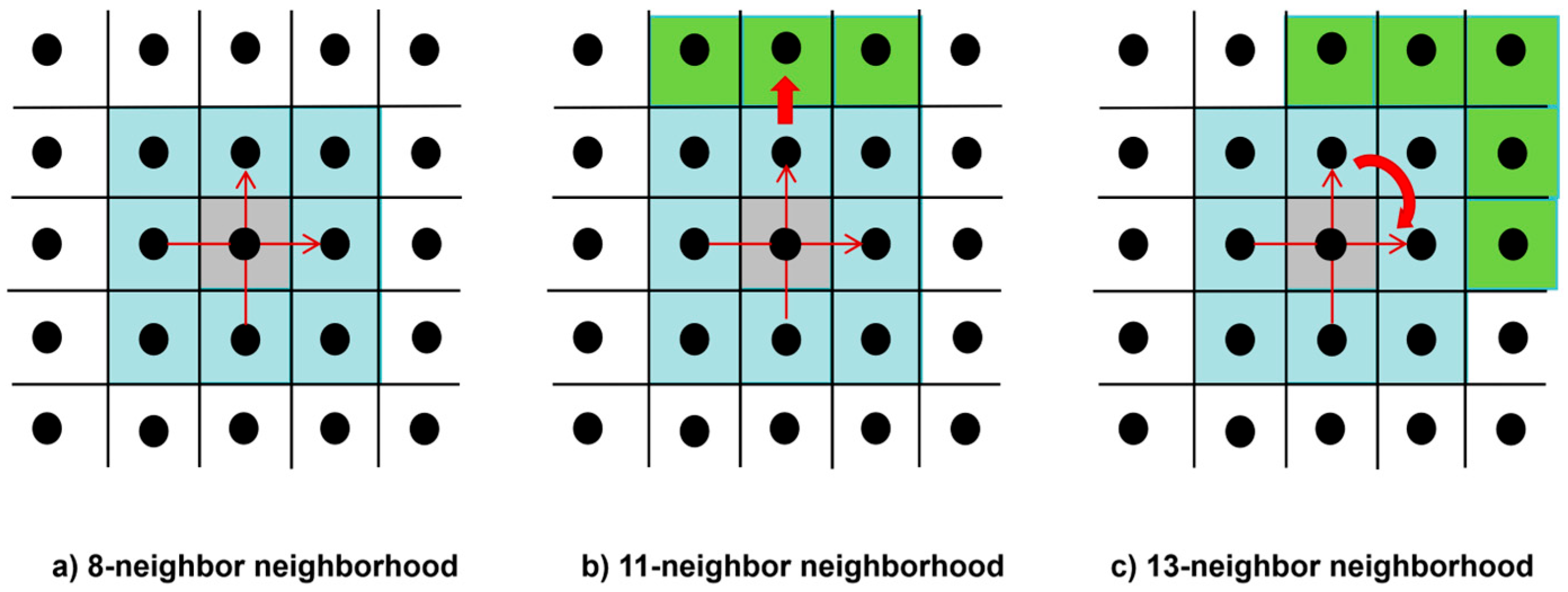
The A* algorithm is a classic heuristic graph search algorithm. Its core lies in evaluating the cost of nodes through the evaluation function $f\left(n\right) = g\left(n\right) + h\left(n\right)$. Here, $g\left(n\right)$ is the actual cumulative cost from the start point to the current node n, and $h\left(n\right)$ is the estimated cost from node n to the target point. The algorithm iteratively searches for the optimal path using an open list and a closed list. In traditional grid maps, node expansion typically employs an 8-neighborhood search strategy, allowing diagonal movements to increase path flexibility. However, the A* algorithm has two obvious problems in complex, large-scale environments. First, the search efficiency is low. The unidirectional search relies on the heuristic function for guidance; when encountering large obstacle areas or local dead ends, it tends to expand a large number of nodes that deviate from the target direction. Second, the path quality is poor. Paths generated by standard A* often contain many sharp corners and redundant turning points, which are unfavorable for the actual driving of intelligent vehicles. To address these issues, this paper introduces an adaptive 8-11-13 variable neighborhood search strategy during the node expansion phase. This strategy can dynamically and directionally adjust the node expansion range based on the position of the target point and surrounding environmental information. Based on Figure 3 below, the specific search and expansion mechanism is as follows:

In the initial stage of node expansion, the algorithm first takes the current node (the central gray-shaded node) as the origin and traverses its 8 adjacent regions (blue grid cells), as shown in Figure 3a. If no obstacles are found within the 8-neighborhood search range, the algorithm determines that the surrounding environment is relatively safe and continues to expand outward. During further expansion, the algorithm calculates a vector originating from the current node and pointing to the final target node. As shown in Figure 3b, when this pointing vector is parallel to a coordinate axis (for example, directly upwards as indicated by the red arrow), the algorithm will additionally expand 3 nodes (green grid cells) in the positive direction of this vector, thereby constituting an 11-neighborhood search. Similarly, as shown in Figure 3c, when the vector pointing to the target point falls within one of the four quadrants of the coordinate system (for example, the upper right quadrant indicated by the red curved arrow), the algorithm will additionally expand 5 nodes (green grid cells) in the direction of the corresponding quadrant, forming a 13-neighborhood search. Through this variable neighborhood mechanism, the TA-BVNS-A* algorithm ensures that node expansion always proceeds toward the direction where the target point is located. This significantly reduces redundant searches that deviate from the target direction and substantially improves the planning efficiency and directionality of the algorithm in complex environments.

5. Global Path Smoothing Based on Bézier Curves

5.1. Path Node Filtering

Although the bidirectional variable neighborhood search A* algorithm improves planning efficiency, the generated paths have issues such as jagged polylines and discontinuous curvature, making it difficult to meet the path smoothness requirements of off-road environments. Therefore, this paper introduces a node filtering mechanism to perform post-processing optimization on the initial path. The specific process is as follows:

• Step 1: Initialization. Set the start point S as the current anchor point A, and add it to the key node set K.
• Step 2: Forward search. Starting from the anchor point A, sequentially connect the subsequent nodes ${\mathit{P}}_{\mathit{i}+1},{\mathit{P}}_{\mathit{i}+2},...,{\mathit{P}}_{\mathit{n}},\mathit{G}$, and verify the traversability of the line segment $\mathit{A}\to {\mathit{P}}_{\mathit{k}}$.
• Step 3: Multiple constraint detection. Perform four tests on the line segment from A to ${\mathit{P}}_{\mathit{k}}$: first, geometric collision testing to ensure the segment does not pass through any obstacle grid cells; second, safety margin testing, requiring the segment to maintain a distance of at least one grid cell from obstacles; third, terrain cost testing to ensure the average cost of the segment area does not exceed 1.5 times that of the corresponding section of the original path; finally, turning capability testing to verify whether a single turning angle is within the vehicle’s maximum steering angle range. Only when all tests are passed will the current anchor point continue to be expanded; otherwise, expansion is immediately terminated.
• Step 4: Key node extraction. Add the last node that passed the tests, ${\mathit{P}}_{\mathit{k}-1}$, to K as a key node, and set it as the new anchor point A.
• Step 5: Iterative execution. Repeat steps 2 to 4 until the anchor point A reaches the target point G, and add G to K.
• Step 6: Path reconstruction. Sequentially connect each node in K to generate the filtered path.

By eliminating redundant nodes, this mechanism shortens the path length and reduces the number of turns while ensuring traversability, providing a high-quality sequence of control points for subsequent Bezier curve smoothing.

5.2. Curve Smoothing and Constraint Processing

The path after node filtering remains a polyline, presenting issues with curvature discontinuity. This paper employs a cubic Bezier curve for smoothing, and the control points are generated as follows:

$$P_0=K_{i+1},$$

(15)

$$P_3=K_{i+2},$$

(16)

$$P_1=P_0+{\alpha }_0\cdot L_S\cdot \overrightarrow{T_0},$$

(17)

$$P_2=P_3-{\beta }_0\cdot L_S\cdot \overrightarrow{T_3},$$

(18)

where $\overrightarrow{{\mathit{T}}_0}={\displaystyle \frac{{\mathit{K}}_{\mathit{i}+1}-{\mathit{K}}_{\mathit{i}}}{‖{\mathit{K}}_{\mathit{i}+1}-{\mathit{K}}_{\mathit{i}}‖}}$ represents the driving direction upon entering the current segment, $\overrightarrow{{\mathit{T}}_3}={\displaystyle \frac{{\mathit{K}}_{\mathit{i}+2}-{\mathit{K}}_{\mathit{i}+1}}{‖{\mathit{K}}_{\mathit{i}+2}-{\mathit{K}}_{\mathit{i}+1}‖}}$ represents the driving direction upon leaving the current segment, and ${\mathit{L}}_{\mathit{S}}=‖{\mathit{K}}_{\mathit{i}+2}-{\mathit{K}}_{\mathit{i}+1}‖$ represents the distance from the start point to the end point of the current segment. ${\mathit{\alpha }}_0,{\mathit{\beta }}_0$ are scaling factors (initial value 0.4, adjusted with a step size of 0.05–0.1, lower limit 0.1). Through control point adjustment, the integration of three types of constraints is achieved:

(1)

Turning constraint: The curve curvature $\mathit{\kappa }\left(\mathit{t}\right)$≤${\displaystyle \frac{1}{{\mathit{R}}_{\mathit{m}\mathit{i}\mathit{n}}}}$, ensuring the minimum turning radius is met.

(2)

Terrain constraint: By adjusting the scaling factors ${\mathit{\alpha }}_0$ and ${\mathit{\beta }}_0$ (step size 0.05), the generated Bezier curve dynamically approximates the original safe polyline. This ensures that the smoothed path does not significantly deviate from the low-cost areas, avoiding intrusion into steep slopes or high-resistance zones.

(3)

Connection constraint: The curvature of adjacent curve segments is continuous, ensuring a smooth transition in the global heading.

Under the premise of ensuring terrain adaptability, this smoothing method achieves continuous curvature, eliminates jagged polylines, guarantees that the maximum path curvature satisfies vehicle constraints, and improves driving smoothness.

6. Integrated System Framework for TA-BVNS-A*

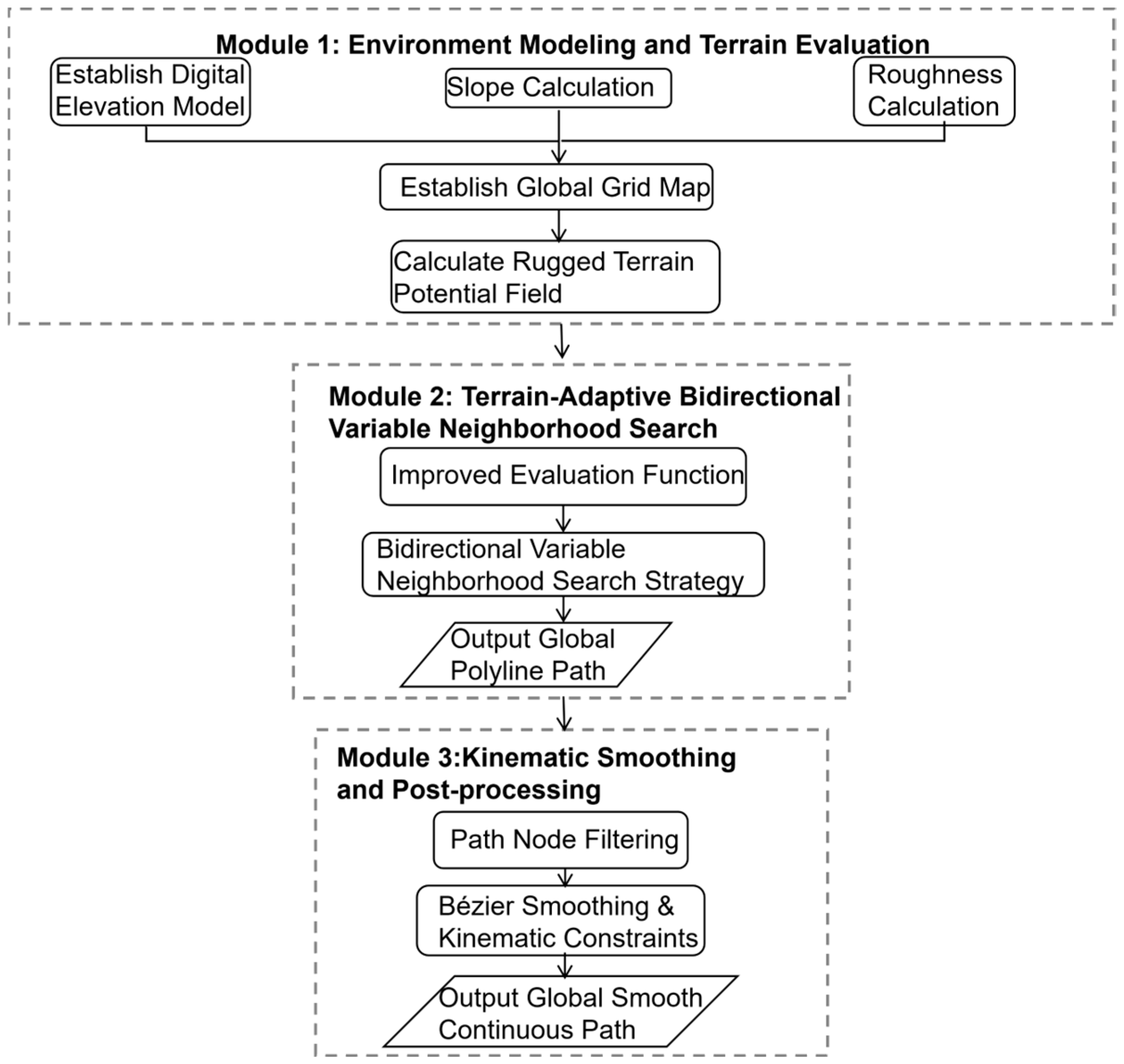
This paper proposes a three-layer progressive path planning framework: first, a terrain cost map is constructed based on a DEM; then, a global polyline path is generated by employing a bidirectional alternating search mechanism, a variable neighborhood search mechanism, and an improved heuristic function mechanism; finally, a continuous path satisfying kinematic constraints is output through node filtering and Bézier smoothing. The three-layer architecture achieves a complete planning process from environment modeling to executable path generation. The framework is illustrated in Figure 4, and it serves as the reference input for the low-level vehicle motion controller.

The proposed TA-BVNS-A* algorithm involves several key technical parameters and mathematical notations. All critical symbols, abbreviations, and parameter settings are consolidated in the ‘Nomenclature and Parameter Settings’ section after the conclusion for clarity and reproducibility.

7. Numerical Simulation Verification

7.1. Numerical Simulation Setup and Evaluation Metrics

To verify the effectiveness of the highly efficient global path planning method proposed in this paper, comparative simulations were conducted in DEM grid maps of varying scales (50 m × 50 m, 100 m × 100 m, and 200 m × 200 m, with a grid resolution of 1 m × 1 m). The map construction is based on the aforementioned off-road environment modeling theory, generating 3D map models and their corresponding 2D planar maps. Different surface conditions are distinguished by color (green for dirt roads, gray for gravel roads, and yellow for sandy terrain). On the basis of the undulating terrain, absolute obstacles with fixed boundaries (such as blue lakes and dark green trees, with elevation values set to infinity and marked as impassable areas) were further configured, thereby constructing an off-road test environment that incorporates terrain slope resistance, surface passage cost, and obstacle collision risk.

In these simulations, the average computation time and the number of search nodes were selected as the core metrics to evaluate the search efficiency of the algorithms. Simultaneously, the maximum front-wheel steering angle and the curvature variation graph were selected to evaluate path smoothness and the ability to satisfy vehicle kinematic constraints. To strictly evaluate computational stability and eliminate the influence of environmental randomness, each specific map scenario (including its randomized surface costs) was generated once and kept static during 30 independent test runs. Because the heuristic search algorithms are deterministic, the expanded search nodes and the final path length remain absolutely constant across these 30 runs on the same map; only the computation time fluctuates due to CPU scheduling. Therefore, the computation time of each algorithm is reported as the “mean ± standard deviation,” while the path length and search nodes are reported as exact constant values.

It should be clarified that the evaluation metrics vary slightly across different tables to reflect the specific focus of each simulation stage. In the global path search evaluation (e.g.,

Table 2. Output metrics of the 3D-A* and TA-A* algorithms on different maps. The average computation time is reported as the mean ± standard deviation over 30 independent runs. The path length represents the exact constant value derived from the static map.

Map Size (m)	Algorithm	Average Time (ms)	Maximum Path Slope (%)	Search Nodes	Path Length (m)
50 × 50	3D-A*	6.88 ± 0.79	26.72	1764	72.53
	TA-A*	6.57 ± 0.26	22.64	739	71.36
100 × 100	3D-A*	25.67 ± 1.80	42.35	6918	157.15
	TA-A*	18.43 ± 0.86	39.90	4159	165.54
200 × 200	3D-A*	139.89 ± 5.76	42.51	29,180	260.84
	TA-A*	187.86 ± 8.80	38.81	14,453	281.56

), “Max Path Slope” is utilized to demonstrate the algorithm’s terrain adaptability and its capability to avoid steep, hazardous areas. In the path smoothing evaluation, “Max Steering Angle” is introduced as a critical metric. Because the smoothing process directly affects path curvature, evaluating the steering angle is essential for verifying kinematic feasibility and smoothness.

This simulation compares the following algorithms: 3D-A*: In the constructed off-road environment, distance cost and slope resistance are considered, but the impacts of surface conditions and undulating topography are not; Terrain-Adaptive A* (TA-A*): Integrates distance cost, slope resistance, and the impacts of surface conditions and undulating topography; Terrain-Adaptive Bidirectional Variable Neighborhood Search A* (TA-BVNS-A*): On the basis of terrain adaptability, it incorporates bidirectional alternating search, exponential weighting, and variable neighborhood search mechanisms.

To ensure the reproducibility of our simulation results, the standardized setup for the three map scales (50 × 50, 100 × 100, and 200 × 200) is defined as follows: the start and goal coordinates are fixed at the diagonal corners of the grid (e.g., [5, 5] and [45, 45] for the 50 × 50 scale). The surface traversal costs are assigned according to the categories in Table 1, where rolling resistance coefficients ${\mathit{f}}_{\mathit{r}}$ are sampled within the specified ranges to simulate environmental randomness. The terrain-adaptive evaluation function utilizes these mapped costs to prioritize safer paths, ensuring the algorithm remains consistent across different map scales.

7.2. Path Analysis of TA-A* Based on Off-Road Environment Modeling

To verify the applicability and superiority of the path planning algorithm proposed in this paper in off-road scenarios, two sets of comparative simulations were designed in this section.

First, a simulation comparison was conducted between the A* algorithm in a 2D map environment and 3D-A* in a 3D map environment. The simulation results, as shown in Figure 5 and Figure 6, indicate that the 2D map can only achieve basic 2D planar obstacle avoidance, completely lacking terrain undulation and elevation information; whereas in 3D terrain, the 3D-A* algorithm, in addition to avoiding rigid obstacles, also considers terrain slope, enabling it to effectively identify complex terrain such as mountains and execute reasonable detours. Because off-road vehicles are vastly affected by terrain elevation in actual driving, 2D planar simulations cannot authentically reflect their traversal constraints; therefore, 2D maps are unsuitable for path planning simulation of off-road vehicles.

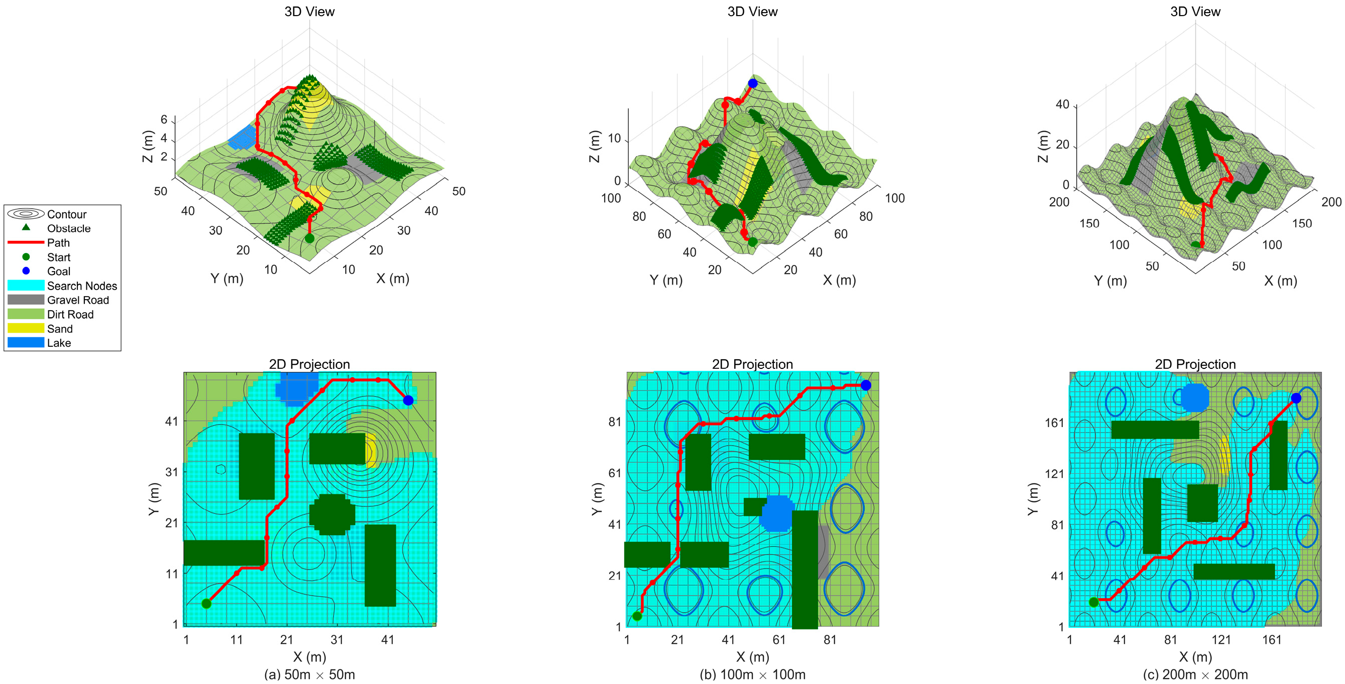
Building upon this, this paper further compares the comprehensive performance of 3D-A* and TA-A* in 3D terrain; the simulation data are presented in Table 2 below. Judging from Figure 6 and Figure 7 and the tabular data, under the premise that the path length and other key evaluation metrics are similar, TA-A* not only possesses global obstacle circumvention capability, but the maximum slope of its planned path and the number of search nodes are significantly lower than those of 3D-A*. A smaller path slope can effectively enhance the driving safety and dynamic smoothness of off-road vehicles in undulating terrain. From the comprehensive analysis above, it is evident that TA-A* exhibits superior terrain adaptability in complex off-road environments.

7.3. Verifying the High Efficiency of the Bidirectional Variable Neighborhood Search

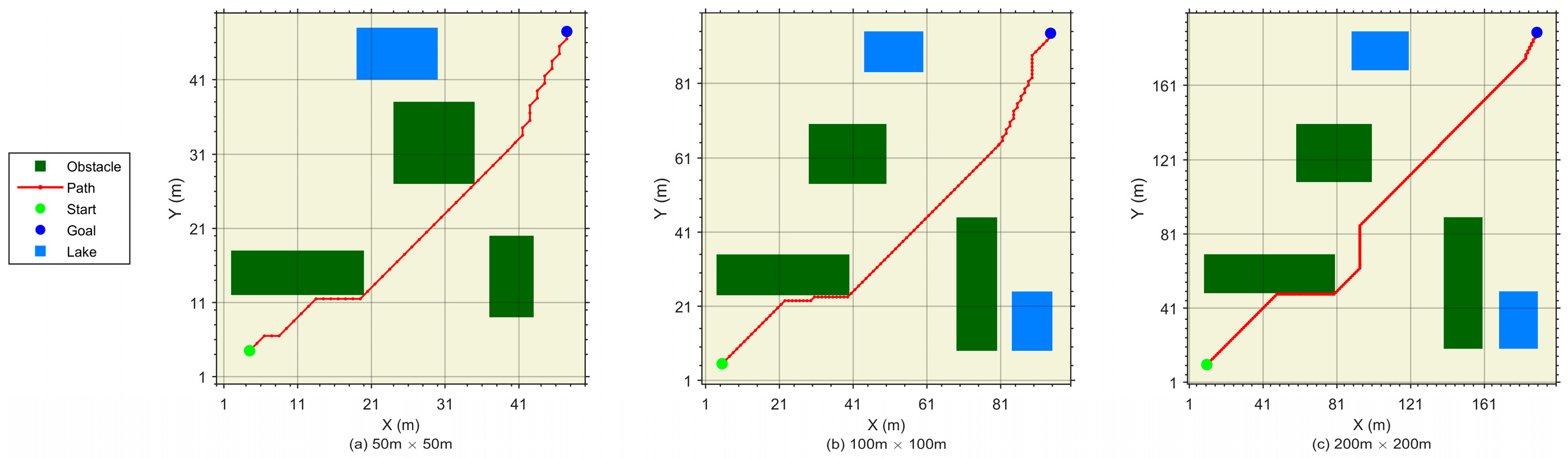
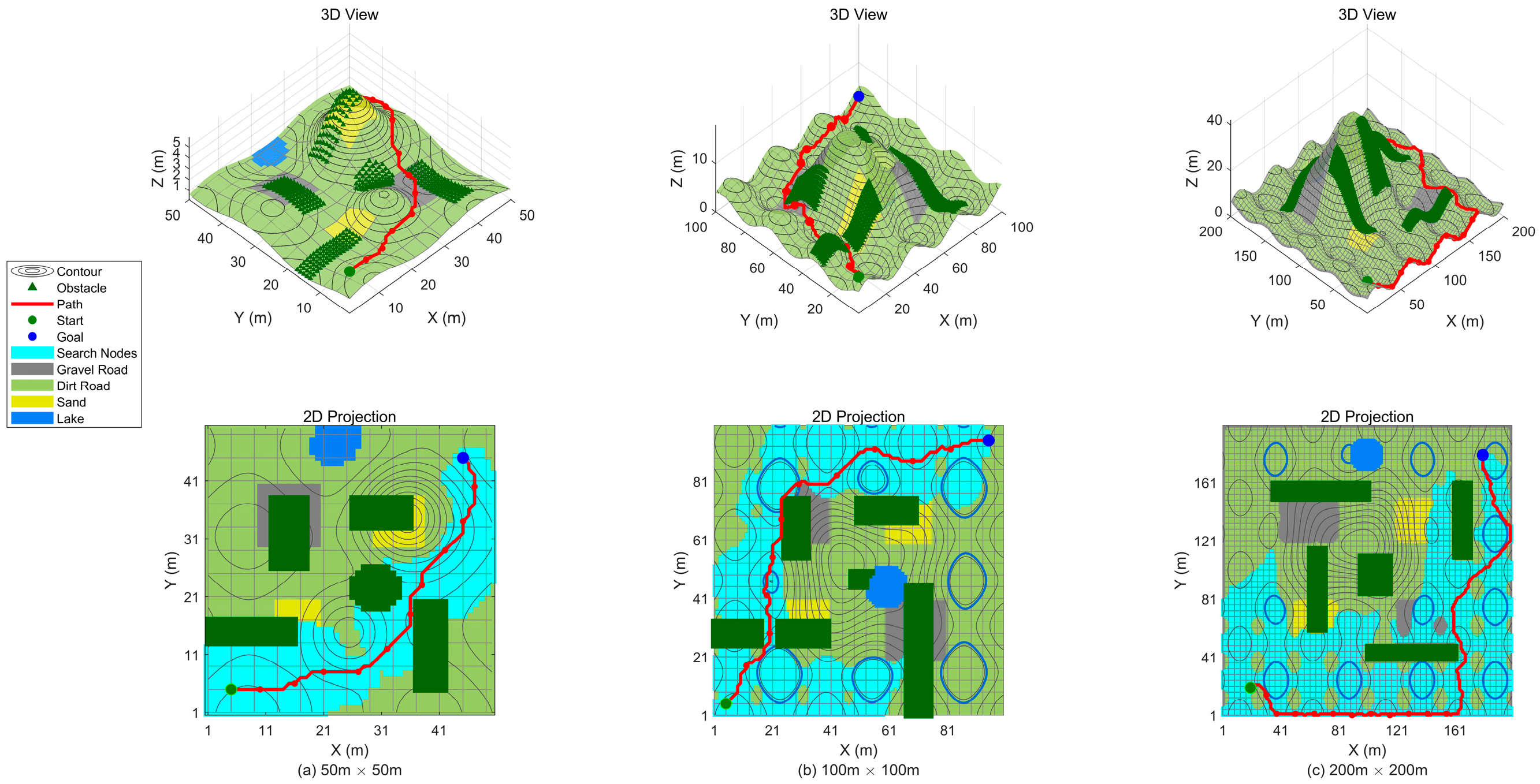
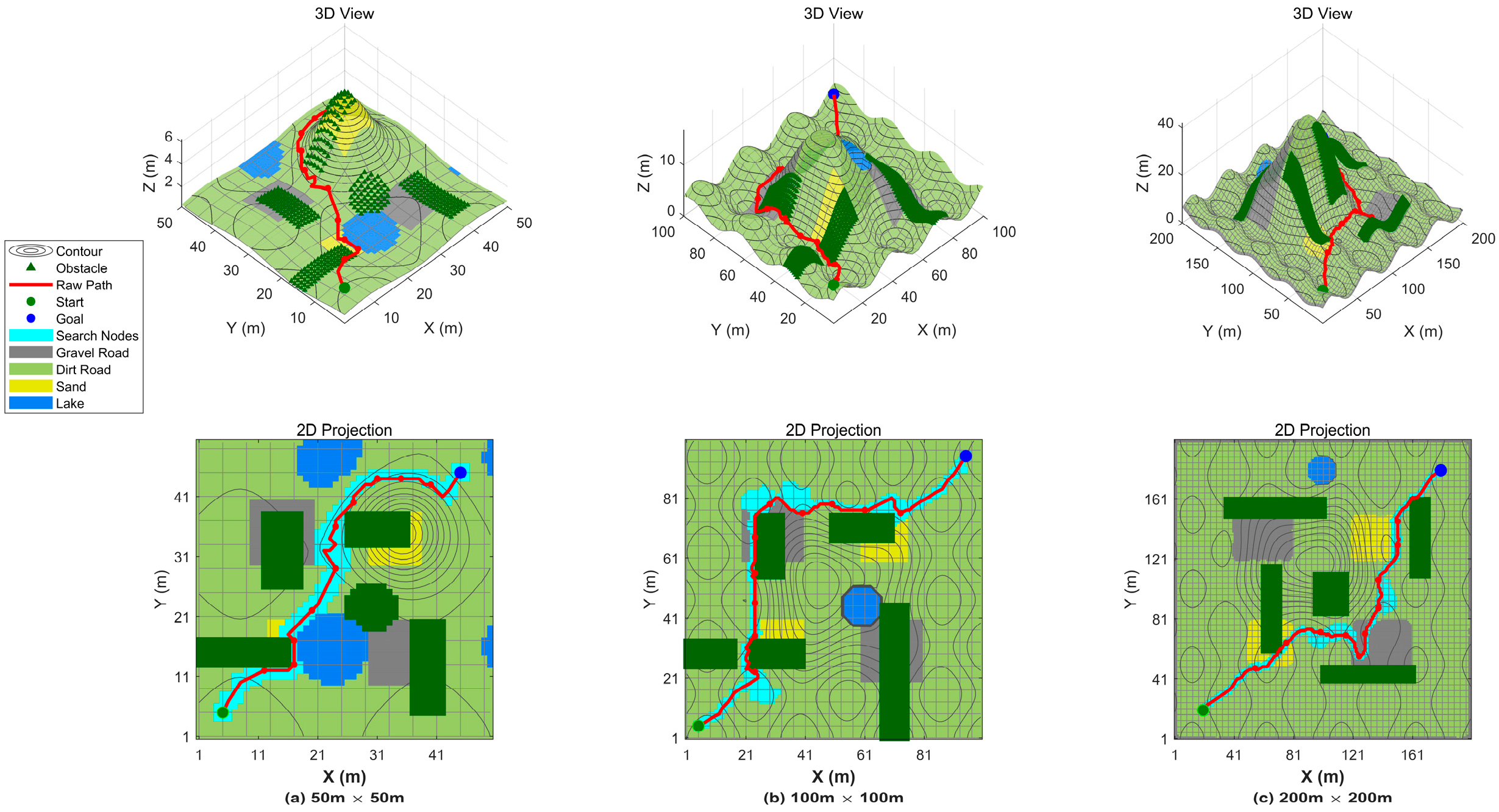
To verify the contributions of the bidirectional search mechanism, variable neighborhood mechanism, and exponential weighting mechanism in improving search efficiency, this section compares the performance of the TA-A* algorithm and the TA-BVNS-A* algorithm across maps of different scales. Figure 7 and Figure 8 respectively display the visual results of path planning under three map sizes, and the quantitative evaluation metrics are shown in

Table 3. Output metrics of the TA-A* and TA-BVNS-A* algorithms on different maps. The average computation time is reported as the mean ± standard deviation over 30 independent runs. The path length represents the exact constant value derived from the static map.

Map Size (m)	Algorithm	Average Time (ms)	Search Nodes	Path Length (m)
50 × 50	TA-A*	6.57 ± 0.26	739	71.36
	TA-BVNS-A*	1.88 ± 0.59	203	72.06
100 × 100	TA-A*	18.43 ± 0.86	4159	165.54
	TA-BVNS-A*	11.11 ± 0.41	687	172.18
200 × 200	TA-A*	187.86 ± 8.80	14,453	281.56
	TA-BVNS-A*	70.38 ± 5.66	1709	298.20

. Analysis of simulation results: The search nodes for the TA-BVNS-A* algorithm (Figure 8) decreased significantly (the cyan areas in the figure). The data show that across all map sizes, the number of search nodes for TA-BVNS-A* experienced a substantial decline compared to TA-A*. Particularly in the 200 m × 200 m complex environment, TA-A* needed to search 14,453 nodes, whereas TA-BVNS-A* only needed to search 1709 nodes, compressing the search nodes by approximately 88.2%. This indicates that the bidirectional search mechanism can effectively avoid the blind expansion generated by unidirectional search. Simultaneously, the computation time of TA-BVNS-A* was also substantially reduced; in the 200 m × 200 m scale environment, its time consumption of 70.38 ms was 62.5% lower than that of TA-A*, while in the 50 m × 50 m map, the average computation time of TA-BVNS-A* was only 1.88 ms, representing a reduction of approximately 71.4% compared to TA-A*. All of this proves that the variable neighborhood search strategy and the exponential weighting mechanism can drastically improve computational efficiency in complex terrain.

7.4. Path Smoothing Effect Analysis

As observed from Figure 8, although terrain adaptability steers the path away from high-cost areas and significantly reduces computation time and search nodes, numerous sharp corners and redundant nodes still exist. To address this issue, integrating the aforementioned theories, this paper adopts a “filtering first, then constrained smoothing” strategy to process the initial path.

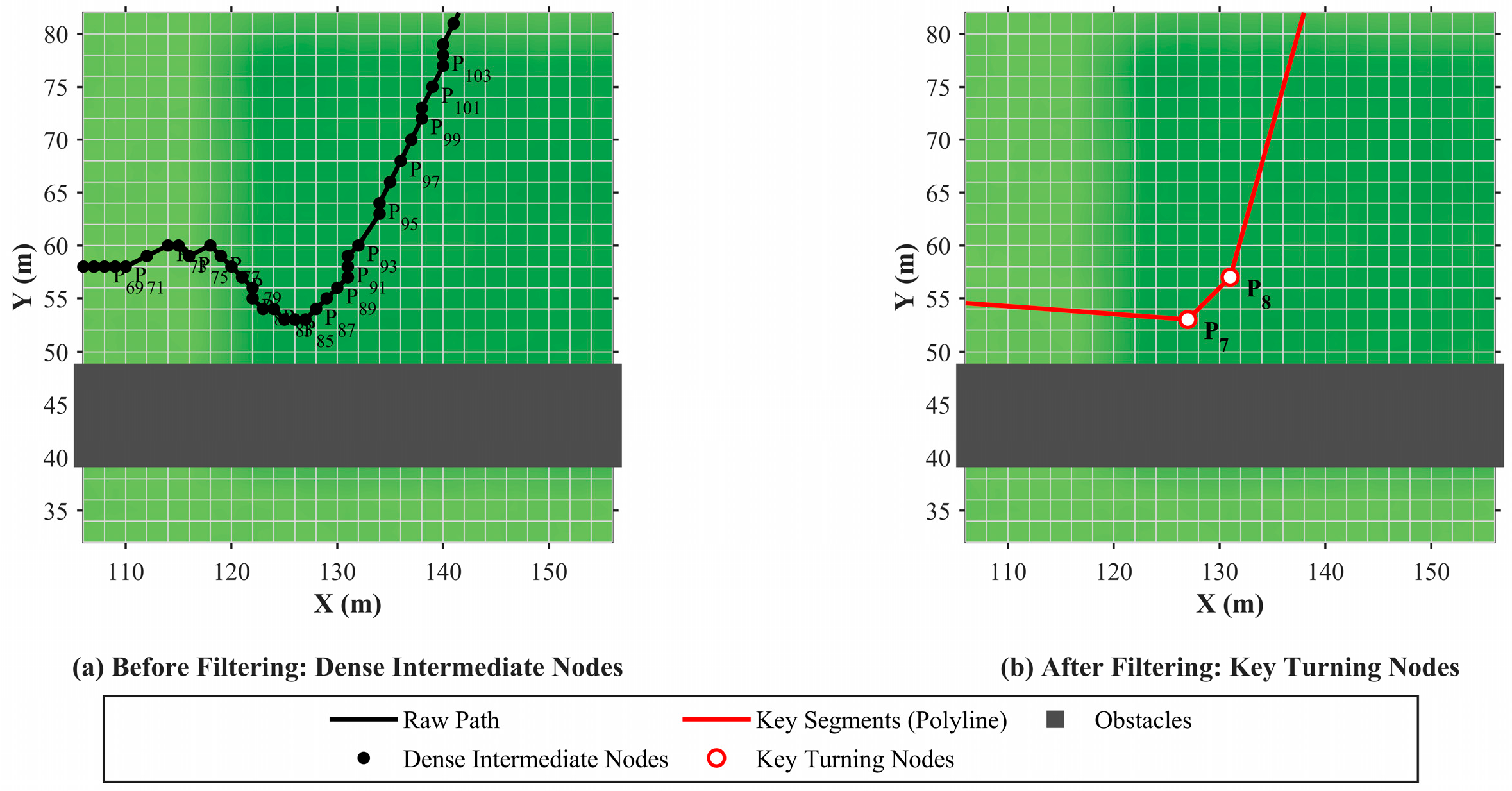
The first step is path node filtering. Figure 9 visually compares the local path details before and after filtering. As shown in Figure 9a, the pre-filtered path contains a massive number of densely packed redundant intermediate nodes, which would cause unnecessary minor steering wheel jitters during actual vehicle tracking. After being processed by the node filtering strategy, as shown in Figure 9b, the algorithm successfully eliminates redundant turning points, retaining only the key inflection nodes that genuinely determine the path. This critical step greatly simplifies the path morphology, removes most of the ineffective jagged polylines, and simultaneously substantially reduces the computational load for subsequent curve fitting.

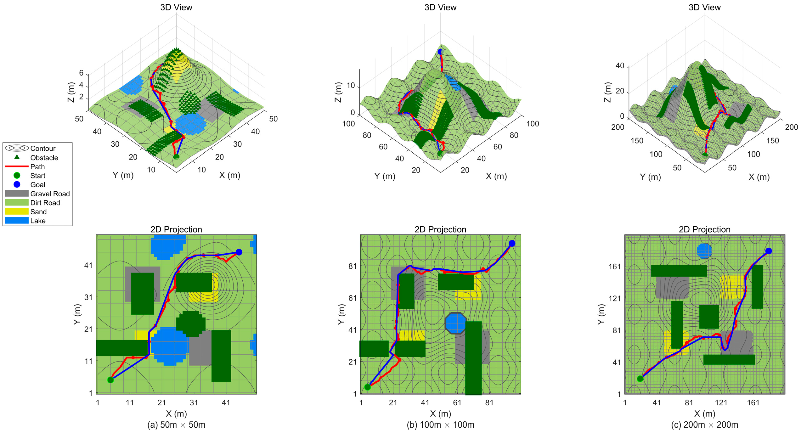
Building upon node filtering, the geometric morphology of the path is further optimized through curve fitting. Figure 10 presents a comparison of the global path generated by the TA-BVNS-A* algorithm before and after smoothing. As can be observed, the unsmoothed initial path (the red path in Figure 10) contains a large number of 45-degree and 90-degree turns, and exhibits discontinuous inflection points at terrain undulations; whereas the smoothed path, TA-BVNS A* (Filtered), better conforms to the terrain’s contours. This improvement in geometric continuity intuitively demonstrates the effectiveness of the smoothing strategy proposed in this paper in eliminating redundant inflection points and enhancing path search quality.

To further quantitatively evaluate the comprehensive performance of the improved algorithm proposed in this paper,

Table 4. Performance improvement rate of the TA-BVNS-A*(Filtered) algorithm compared to other algorithms under different map scenarios. The path length represents the exact constant value derived from the static map.

Map Size (m)	Algorithm	Average Time (ms)	Max. Steering Angle ($°$)	Search Nodes	Path Length (m)
50 × 50	3D-A*	6.88 ± 0.79	45.00	1764	72.53
	TA-A*	6.57 ± 0.26	45.00	739	71.36
	TA-BVNS A*	1.88 ± 0.59	90.00	203	72.06
	TA-BVNS A* (Filtered)	8.24 ± 0.32	33.68	203	73.35
100 × 100	3D-A*	25.67 ± 1.80	45.00	6918	157.15
	TA-A*	18.43 ± 0.86	90.00	4159	165.54
	TA-BVNS A*	11.11 ± 0.41	90.00	687	172.18
	TA-BVNS A* (Filtered)	13.05 ± 1.53	31.36	687	162.02
200 × 200	3D-A*	139.89 ± 5.76	45.00	29,180	260.84
	TA-A*	187.86 ± 8.80	90.00	14,453	281.56
	TA-BVNS A*	70.38 ± 5.66	90.00	1709	298.20
	TA-BVNS A* (Filtered)	73.46 ± 3.88	32.60	1709	269.33

details the evaluation metrics of each algorithm across different map scales. Simulation data indicate that, compared to the TA-BVNS-A* algorithm without constraint processing, the algorithm subjected to node filtering and smoothing constraints exhibits significant advantages in the key metric of the maximum front-wheel steering angle. For instance, in the 200 m × 200 m complex environment detailed, the maximum front-wheel steering angle decreases from 90° (unfiltered) to 32.6° (filtered). This represents a significant reduction of 63.78% (calculated as (90 − 32.6)/90 × 100%), substantially enhancing path executability and vehicle driving smoothness.

It is worth noting that, as observed in the simulation results (such as in Table 3 and the various map scenarios in Table 4), the path length generated by the proposed TA-BVNS-A* algorithm is occasionally slightly longer than that of the baseline algorithms. This phenomenon directly reflects the trade-off between computational efficiency and path optimality discussed in Section 4.2. TA-BVNS-A* prioritizes a near-optimal and highly safe traversal path over the traditional blind pursuit of the shortest distance. In real-time off-road driving, this minor increase in path length is a reasonable and worthwhile compromise in exchange for a substantial improvement in vehicle safety.

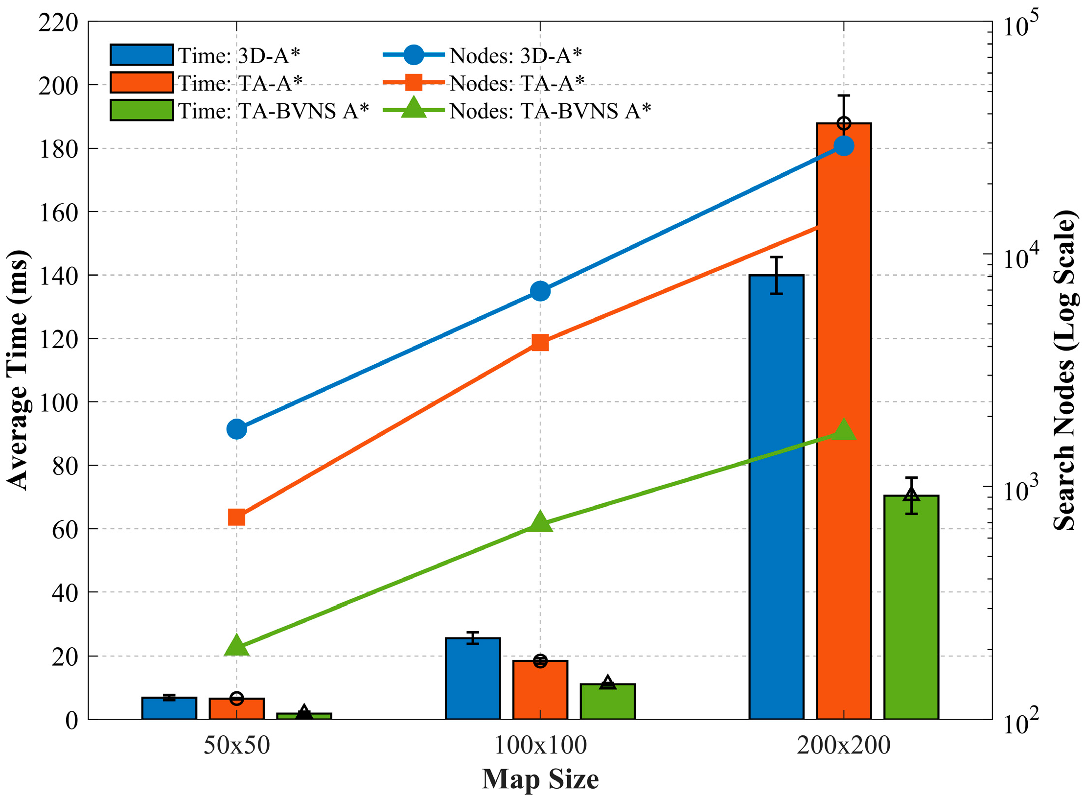
To provide a more intuitive evaluation of the computational efficiency of each algorithm, Figure 11 presents a joint dual-axis statistical analysis. The left Y-axis uses grouped bar charts with standard deviation error bars to compare the average execution time, while the right Y-axis plots the total number of expanded search nodes across varying map dimensions on a logarithmic scale. As observed from Figure 11, the baseline 3D-A* algorithm suffers from a significant increase in both search space and computation time as the environment scale grows, whereas the proposed TA-BVNS-A* algorithm demonstrates superior scalability. In the 200 × 200 complex map scenario, the proposed method limits the expansion of redundant search nodes to a highly constrained level, thereby achieving stable, real-time computational performance that significantly outperforms the comparative frameworks.

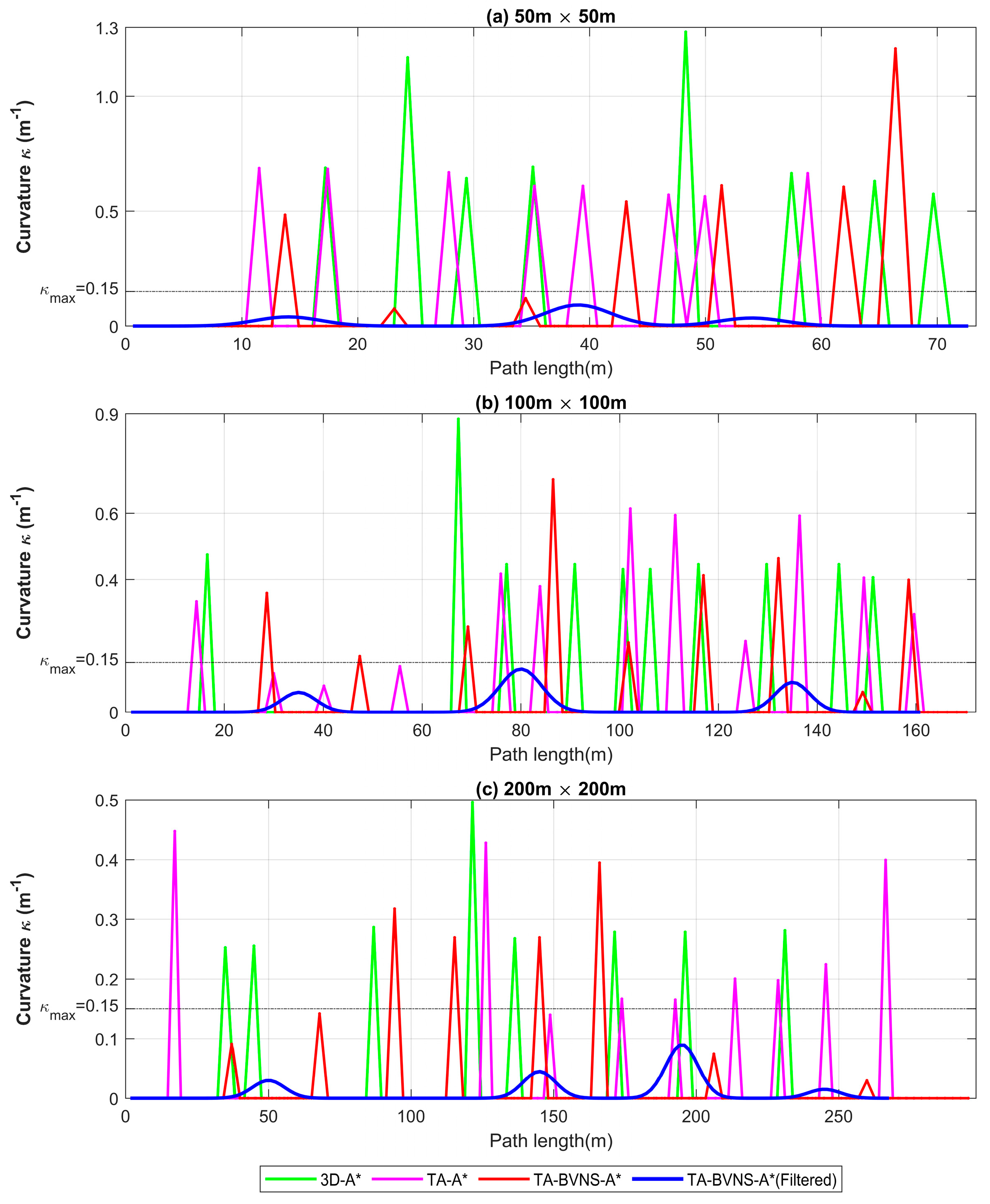
Figure 12 illustrates the curvature variation curves of the unsmoothed path generated by the previously mentioned simulation algorithm against the path length across three map scales. The horizontal dashed line in the figure represents the vehicle’s physical curvature limit of 0.15. As can be seen from the figure, the curvature of the unsmoothed paths (red, green, and purple dashed lines) exhibits a massive number of severe, pulse-like abrupt changes, with multiple peaks far exceeding the constraint limit of 0.15. This curvature discontinuity implies that the intelligent off-road vehicle would need to instantaneously turn the steering wheel to its limit position during travel, which is physically unfeasible and would induce severe mechanical vibrations. In contrast, the optimized smoothed path (blue solid line) demonstrates excellent continuity. Across all map scenarios, the curvature fluctuations of the smoothed path remain below the maximum curvature limit, and the curvature change gradient is gentle. This indicates that the path satisfies the travel continuity requirements, ensuring that variations in the front-wheel steering angle are continuous and constrained, thereby significantly enhancing the driving stability of the intelligent off-road vehicle in complex off-road environments.

8. Conclusions

In this paper, we proposed the TA-BVNS-A* algorithm to address the global path planning challenges for intelligent vehicles in complex off-road environments. By integrating a bidirectional alternating search strategy with a variable neighborhood mechanism, the proposed method effectively mitigates the blind expansion issues of traditional A* algorithms. Simulation results demonstrate that TA-BVNS-A* significantly enhances search efficiency and path executability while maintaining superior terrain adaptability. To bridge the gap between theoretical algorithmic optimization and practical engineering, future research will focus on three key areas: (1) conducting Hardware-in-the-Loop (HIL) testing on embedded units (e.g., Infineon AURIX TC264) to validate real-time performance; (2) expanding terrain complexity models via multi-sensor fusion; and (3) performing comprehensive outdoor field tests on physical vehicle platforms.

References

1. Vice, J.M.; Sukthankar, G. DUnE: A Versatile Dynamic Unstructured Environment for Off-Road Navigation. Robotics 2025, 14, 35. [Google Scholar] [CrossRef] [Scilit]
2. Jamwal, H.D.S.; Singh, S. Comprehensive Survey on Autonomous Disaster Reconnaissance: A Comparative Analysis of UAVs and UGVs. Telecom 2026, 7, 31. [Google Scholar] [CrossRef] [Scilit]
3. Shen, Y.; Shen, Y.; Zhang, Y.; Huo, C.; Shen, Z.; Su, W.; Liu, H. Research Progress on Path Planning and Tracking Control Methods for Orchard Mobile Robots in Complex Scenarios. Agriculture 2025, 15, 1917. [Google Scholar] [CrossRef] [Scilit]
4. Choi, D.; Kang, T. Feeling the Force: A Nuanced Physics-based Traversability Sensor for Navigation in Unstructured Vegetation. IEEE Robot. Autom. Lett. 2025, in press. [Google Scholar] [CrossRef] [Scilit]
5. Han, T.; Liu, A.; Li, A.; Spitzer, A.; Shi, G.; Boots, B. Model Predictive Control for Aggressive Driving Over Uneven Terrain. In Proceedings of the Robotics: Science and Systems (RSS), Delft, The Netherlands, 15–19 July 2024. [Google Scholar] [CrossRef] [Scilit]
6. Venu, S.; Gurusamy, M. A Comprehensive Review of Path Planning Algorithms for Autonomous Navigation. Results Eng. 2025, 28, 107750. [Google Scholar] [CrossRef] [Scilit]
7. Sultana, S.S.; Tanabe, T.; Fausten, T.; Irie, M. Avoiding Premature Convergence to Local Optima with Adaptive Exploration for Genetic Algorithms. In Proceedings of the Genetic and Evolutionary Computation Conference Companion (GECCO 2025), New York, NY, USA, 14–18 July 2025. [Google Scholar] [CrossRef] [Scilit]
8. Cicirello, V.A. Self-Tuning Lam Annealing: Learning Hyperparameters While Problem Solving. Appl. Sci. 2021, 11, 9828. [Google Scholar] [CrossRef] [Scilit]
9. Yu, M.; Luo, Q.; Xiao, Q. Research Review Based on Improved Ant Colony Algorithm. In Proceedings of the 2022 International Conference on Wireless Communications, Networking and Applications (WCNA 2022), Wuhan, China, 16–18 December 2022; Springer: Singapore, 2022. [Google Scholar] [CrossRef] [Scilit]
10. Kennedy, J.; Eberhart, R.C. Particle Swarm Optimization. In Proceedings of the 1995 IEEE International Conference on Neural Networks (ICNN), Perth, WA, Australia, 27 November–1 December 1995; IEEE: New York, NY, USA, 1995; Volume 4. [Google Scholar] [CrossRef] [Scilit]
11. Zhang, Y.; Liang, H.; Li, J. Research on UAV Path Planning Based on Improved Dijkstra’s Algorithm. Int. J. Hous. Sci. Appl. 2025, 46, 7473–7482. [Google Scholar] [CrossRef] [Scilit]
12. Hart, P.E.; Nilsson, N.J.; Raphael, B. A Formal Basis for the Heuristic Determination of Minimum Cost Paths. IEEE Trans. Syst. Sci. Cybern. 1968, 4, 100–107. [Google Scholar] [CrossRef] [Scilit]
13. Harabor, D.; Grastien, A. Online Graph Pruning for Pathfinding on Grid Maps. In Proceedings of the AAAI Conference on Artificial Intelligence, San Francisco, CA, USA, 7–11 August 2011; Volume 25, pp. 1114–1119. [Google Scholar] [CrossRef] [Scilit]
14. Zhang, L.; Zhang, Y.; Zeng, M.; Li, Y. Robot Navigation Based on Improved A* Algorithm in Dynamic Environment. Assem. Autom. 2021, 41, 419–430. [Google Scholar] [CrossRef] [Scilit]
15. Zhang, R.; Zhou, L.; Liu, Z. Path Planning of Mobile Robot Based on MOBDB-RRT* Algorithm. Electron Opt. Control 2022, 29, 12–17. [Google Scholar]
16. Ayawli, B.B.K.; Appiah, A.Y.; Nti, I.K.; Kyeremeh, F.; Ayawli, E.I. Path Planning for Mobile Robots Using Morphological Dilation Voronoi Diagram Roadmap Algorithm. Sci. Afr. 2021, 12, e00745. [Google Scholar] [CrossRef] [Scilit]
17. Lai, X.C.; Mamun, A.A.; Ge, S.S. Polar Polynomial Curve for Smooth, Collision-Free Path Generation Between Two Arbitrary Configurations for Nonholonomic Robots. In Proceedings of the 2007 IEEE 22nd International Symposium on Intelligent Control (ISIC), Singapore, 1–3 October 2007; IEEE: New York, NY, USA, 2007. [Google Scholar] [CrossRef] [Scilit]
18. Nie, S.; Liu, H.; Liao, Z.; Xie, Y.; Xiang, C.; Han, L.; Lin, S. Study on Path Planning for Off-Road Autonomous Vehicles in Complex Terrains. J. Mech. Eng. 2024, 60, 261–272. [Google Scholar] [CrossRef] [Scilit]
19. Chen, X.; Wang, L.; Ma, G.; Zhang, L.; Bao, J.; Jing, H. Path Planning for Unmanned Vehicles in Off-Road Environments Considering Energy Consumption and Stability. J. Automot. Saf. Energy 2025, 16, 496–503. [Google Scholar] [CrossRef]
20. Li, C.; Huang, X.; Ding, J.; Song, K.; Lu, S. Global Path Planning Based on a Bidirectional Alternating Search A* Algorithm for Mobile Robots. Comput. Ind. Eng. 2022, 168, 108123. [Google Scholar] [CrossRef] [Scilit]
21. Li, P.; Li, Y.; Dai, X. VNS–BA*: An Improved Bidirectional A* Path Planning Algorithm Based on Variable Neighborhood Search. Sensors 2024, 24, 6929. [Google Scholar] [CrossRef] [Scilit] [PubMed]
22. Bu, X.; Su, H.; Zou, W.; Wang, P.; Zhou, H. Smooth Path Planning Based on Non-uniformly Modeling and Cubic Bezier Curves. Acta Autom. Sin. 2017, 43, 710–724. [Google Scholar] [CrossRef]
23. Zhao, Y.; Zhang, Q.; Yu, T.; Lin, X.; Zhang, Y.; Li, Y.; Ji, J. Research on Obstacle Avoidance Path Planning Methods for Intelligent Vehicles. J. Nanjing Univ. Sci. Technol. 2023, 47, 148–154. [Google Scholar] [CrossRef]
24. Yu, Z. Automotive Theory, 6th ed.; China Machine Press: Beijing, China, 2018; p. 9. [Google Scholar]
25. Rada, J.; Rybansky, M.; Dohnal, F. The Impact of the Accuracy of Terrain Surface Data on the Navigation of Off-Road Vehicles. ISPRS Int. J. Geo-Inf. 2021, 10, 106. [Google Scholar] [CrossRef] [Scilit]
26. Zhai, L.; Liu, C.; Zhang, X.; Wang, C. Local Trajectory Planning for Obstacle Avoidance of Unmanned Tracked Vehicles Based on Artificial Potential Field Method. IEEE Access 2024, 12, 19665–19681. [Google Scholar] [CrossRef] [Scilit]
27. Xu, B. Precise Path Planning and Trajectory Tracking Based on Improved A-Star Algorithm. Meas. Control 2024, 57, 1025–1037. [Google Scholar] [CrossRef] [Scilit]
Figure 1. Example of elevation value storage.
Actuators 15 00393 g001
Figure 2. Moving Window.
Actuators 15 00393 g002
Figure 3. Illustration of Variable Neighborhood Search. (a) 8-neighbor neighborhood; (b) 11-neighbor neighborhood; (c) 13-neighbor neighborhood. The central gray node represents the current node, the blue cells represent the initial 8-neighborhood search range, and the green cells indicate the additionally expanded nodes. The straight red arrow indicates the vector pointing towards the target node parallel to a coordinate axis, while the red curved arrow indicates the quadrant where the target node is located.
Actuators 15 00393 g003
Figure 4. Global path planning framework for off-road vehicles based on TA-BVNS-A*.
Actuators 15 00393 g004
Figure 5. Path Planning Results of the A* Algorithm on Three Different Map Sizes. (a) 50 m × 50 m map; (b) 100 m × 100 m map; (c) 200 m × 200 m map.
Actuators 15 00393 g005
Figure 6. Path Planning Results of the 3D-A* Algorithm on Three Different Map Sizes. (a) 50 m × 50 m map; (b) 100 m × 100 m map; (c) 200 m × 200 m map.
Actuators 15 00393 g006
Figure 7. Path Planning Results of the TA-A* Algorithm on Three Different Map Sizes. (a) 50 m × 50 m map; (b) 100 m × 100 m map; (c) 200 m × 200 m map.
Actuators 15 00393 g007
Figure 8. Path Planning Results of the TA-BVNS-A* Algorithm on Three Different Map Sizes. (a) 50 m × 50 m map; (b) 100 m × 100 m map; (c) 200 m × 200 m map.
Actuators 15 00393 g008
Figure 9. Local Path Comparison Before and After Node Filtering.
Actuators 15 00393 g009
Figure 10. Comparison of TA-BVNS-A* Algorithm Paths Before and After Smoothing. (a) 50 m × 50 m map; (b) 100 m × 100 m map; (c) 200 m × 200 m map.
Actuators 15 00393 g010
Figure 11. Computational efficiency across different map scales.
Actuators 15 00393 g011
Figure 12. Algorithm Path Curvature Variation Plot. (a) 50 m × 50 m map; (b) 100 m × 100 m map; (c) 200 m × 200 m map.
Actuators 15 00393 g012