Finite-Interval Robust Coefficient Design for Six-Sample Sculling Compensation in UAV Strapdown INS Velocity Updating

Abstract

Accurate onboard velocity updating is essential for UAV strapdown inertial navigation, especially under GNSS-degraded and high-dynamic conditions. Instead of relying only on local Taylor-series cancellation as λ → 0 or directly transferring coning compensation coefficients, the proposed method redesigns velocity-specific sculling coefficients over the finite dimensionless interval λ = ΩΔT ∈ [0, 1]. A two-stage strategy is developed. Stage I constructs a low-cost proxy error model from the analytical expansion and applies a minimax criterion to generate robust candidate coefficients. Stage II further refines them by minimizing a multi-condition time-domain RMS sculling error. Attitude-transfer coefficients are also tested to assess the transferability of optimized coning coefficients to velocity sculling compensation. Under a stringent single-frequency sculling protocol, the velocity-specific Stage-II coefficients reduce the global RMS and worst-case errors by 12.57% and 14.20%, respectively, compared with the classical six-sample coefficients. Under constant specific-force bias, constant angular-rate bias, and double-frequency sculling, the reductions remain 10.62–12.44% and 12.29–16.17%. Ablation and reproducibility checks show that the main gain comes from Stage-II time-domain RMS refinement and remains stable under grid, reference-integration, and base-index variations.

1. Introduction

Inertial navigation systems (INSs) are widely used in unmanned aerial vehicles (UAVs) because of their autonomy, resistance to external interference, and independence from external infrastructure. In environments such as urban canyons, complex terrain, indoor–outdoor transition areas, and satellite-denied or signal-degraded regions, INSs provide a key means of maintaining continuous autonomous navigation [1,2]. However, in pure inertial navigation, navigation errors inevitably accumulate over time due to the absence of external aiding [3]. For highly dynamic UAVs, rapid attitude changes and complex vibration further amplify the influence of discrete algorithmic errors and their propagation [4,5,6,7]. As inertial sensor performance continues to improve, especially with the development of low-drift inertial sensing technologies, algorithmic errors are becoming an increasingly important factor limiting further accuracy improvement under high-dynamic conditions [8,9].

For UAV platforms, such algorithmic errors are not only of theoretical interest but also directly related to onboard navigation reliability. Small and medium UAVs often operate with limited payload capacity, compact IMUs, and highly dynamic motion profiles. During aggressive maneuvers, turning flight, take-off and landing, or operation in GNSS-degraded environments, the onboard INS must maintain continuous velocity and position propagation using sampled inertial increments. In this context, improving the accuracy of the velocity-updating algorithm is important for enhancing the robustness of UAV autonomous navigation.

Strapdown inertial navigation generally consists of attitude updating, velocity updating, and position updating. Velocity updating lies in the middle of this computation chain: it depends on the upstream attitude solution and specific-force measurements, while directly affecting the subsequent position solution [3,4,10]. Under coupled angular and translational motion, discrete sampling, angular-rate integration approximation, and rotational noncommutativity lead to coupling between angular increments and velocity increments, resulting in sculling errors [5,6,10,11]. These errors are representative and challenging in high-dynamic velocity updating and are therefore commonly used to evaluate velocity-update algorithms [4,6]. Multi-sample sculling compensation has been widely adopted to suppress such errors, where the compensation model and its coefficient design play a central role. Since velocity-update errors further propagate into position updating, improving sculling compensation accuracy is important for the overall navigation performance. Reliable numerical evaluation under such conditions also requires high-fidelity reference trajectories and IMU signal generation.

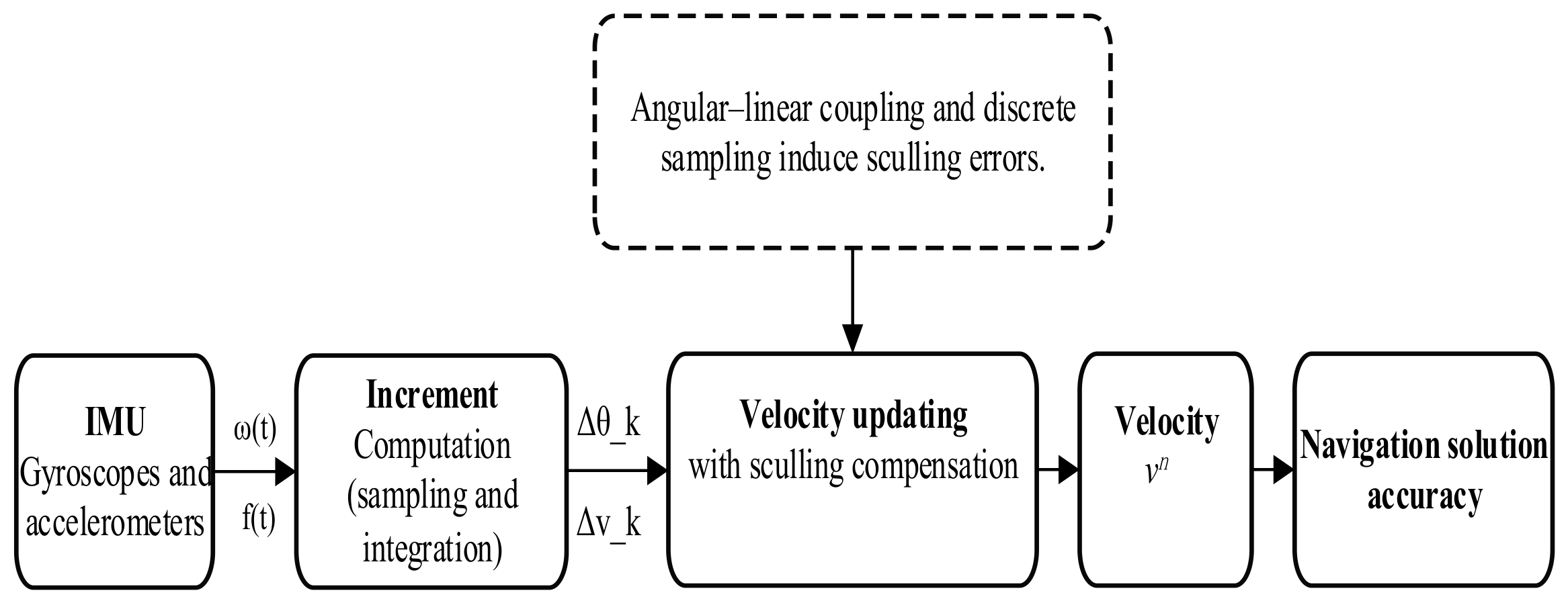
The role of sculling compensation in strapdown inertial velocity updating is illustrated in Figure 1. Angular-rate and specific-force outputs from the IMU are sampled and integrated into angular and velocity increments. When angular and translational motions coexist, the coupling between these increments produces sculling errors. Sculling compensation acts directly in the velocity-updating step; therefore, its accuracy affects not only the velocity solution but also the subsequent position solution and overall navigation performance.

To improve velocity-updating accuracy, multi-sample sculling compensation algorithms have been developed. Their basic idea is to construct compensation terms from multiple angular and velocity increments and to suppress the velocity error caused by discrete sampling and rotational noncommutativity [4,10,11,12,13,14]. The classical three-sample sculling algorithm provides a representative starting point, and later studies extended this idea to higher-sample schemes. In general, increasing the number of subsamples can enhance error suppression, but it also makes coefficient design more complicated [15,16,17,18,19]. The six-sample scheme is therefore of particular interest: it preserves the classical multi-sample velocity-updating framework while providing additional degrees of freedom for coefficient optimization. Moreover, the derivation and expression of some high-sample classical coefficients are not always fully unified or transparent in the literature. This motivates the establishment of a clear and reproducible six-sample baseline before finite-interval robust coefficient redesign.

As the performance limitations of multi-sample compensation algorithms have become better understood, several studies have moved beyond the traditional local design philosophy based only on the small-parameter limit. Savage’s explicit frequency shaping (EFS) method showed that compensation coefficients need not be designed solely by local error cancellation near zero frequency but can instead be optimized over a prescribed frequency range [20]. Analytical studies by Ignagni and co-workers further examined the drift and frequency-response characteristics of velocity and sculling compensation algorithms under oscillatory inputs, indicating that local small-parameter expansions alone cannot fully describe finite-frequency performance [6,11,21]. In addition, alternative computational routes have also been explored. For example, Wu’s iNavFIter method, based on functional iterative integration, provides a fundamentally different approach to high-accuracy inertial navigation, and was later summarized as part of the evolution of inertial navigation computation structures [22,23].

Compared with the above finite-frequency and alternative inertial-computation methods, the present work has a different objective, error metric, and implementation scope. Savage’s EFS method explicitly designs compensation coefficients by shaping the frequency response of strapdown compensation algorithms over a prescribed frequency range, thereby extending coefficient design beyond local zero-frequency cancellation. The related frequency-response analyses also provide important insight into finite-frequency drift and oscillatory-input behavior. By contrast, the present study does not formulate the six-sample sculling problem as a frequency-response shaping problem, nor does it introduce a new online inertial integration structure. Instead, it keeps the classical six-sample sculling compensation structure based on sampled angular and velocity increments and redesigns its fixed coefficients for UAV strapdown INS velocity updating over a prescribed finite dimensionless interval. The proposed Stage-I proxy minimax and Stage-II time-domain RMS refinement provide a velocity-specific coefficient redesign route within the existing multi-sample sculling framework. The final evaluation is performed using multi-condition time-domain sculling compensation errors over different λ values, initial phases, and aggregation bases, rather than only local Taylor-series cancellation or explicit frequency-response shaping.

Nevertheless, for practical strapdown velocity updating based on sampled angular and velocity increments, the classical multi-sample sculling compensation framework remains valuable because of its mature analytical structure, direct compatibility with discrete incremental measurements, and relatively straightforward implementation. The key issue is therefore not whether the classical multi-sample framework should be abandoned, but how its coefficient design can be extended beyond local optimization in the small-parameter neighborhood. Classical sculling compensation coefficients are usually derived by expanding the error near λ = 0 and canceling several leading-order terms; the classical three-sample algorithm is a representative example of this principle. Although theoretically well established, such optimality is essentially local. When the dimensionless parameter λ = ΩΔT enters a moderate range, higher-order terms become more influential, and the resulting coefficients may no longer provide uniformly good performance over the prescribed working interval. Therefore, for six-sample sculling compensation, it is necessary to establish a clear and reproducible classical baseline and then reconsider coefficient design from the perspective of finite-interval robustness over λ ∈ [0, 1].

For engineering interpretation, λ = ΩΔT should be understood as a dimensionless measure of the excitation frequency relative to the subsample interval, rather than as the angular-rate amplitude itself. With the six-sample velocity-update setting used in this study, T = 0.1 s and ΔT = T/6 = 0.0167 s. Therefore, the representative range λ = 0.3–0.8 corresponds to Ω = 18–48 rad/s, or approximately 2.9–7.6 Hz. This range represents medium-to-high finite-step excitation conditions in the present sculling compensation model and is relevant to UAV velocity updating under maneuvering, turning motion, rotor-induced vibration, and structural oscillation components. In this range, residual sculling compensation errors are directly introduced into each velocity update and may further propagate into velocity and position errors in pure inertial navigation. Therefore, reducing the RMS and worst-case sculling errors in this interval has practical significance for improving the robustness of onboard UAV strapdown INS velocity updating.

To address the above issues, this paper revisits the six-sample sculling compensation coefficient design from the perspective of finite-interval robustness. Since the classical derivations of high-sample sculling schemes are not always presented in a clear, unified, and reproducible form, the classical three-sample construction is first briefly reviewed, and a reproducible six-sample baseline is then established as a reference for subsequent optimization. On this basis, coefficient design is no longer restricted to local optimality in the small-parameter neighborhood but is reformulated as a finite-interval robust optimization problem to improve the uniformity and robustness of compensation performance over the prescribed working interval.

A two-stage design strategy is proposed. In the first stage, robust candidate coefficients with improved worst-case behavior over the design interval are generated. In the second stage, these candidates are further refined through multi-condition time-domain simulations to reduce the overall root-mean-square (RMS) sculling compensation error. In addition to the classical baseline, attitude-transfer coefficients, velocity-specific redesigned coefficients, and stage-wise optimized coefficients are included in a unified comparison framework to evaluate their finite-interval performance.

The main contributions of this paper are summarized as follows:

(1)

A clear and reproducible classical six-sample baseline is established. Specifically, the standard three-sample sculling compensation derivation is briefly reviewed, and the classical six-sample coefficient form is derived in a systematic manner.

(2)

The six-sample sculling compensation coefficient design problem is reformulated from local Taylor-series cancellation near the small-parameter limit to finite-interval robust optimization over λ ∈ [0, 1], where λ = ΩΔT characterizes the finite-step effect in velocity updating. Thus, coefficient evaluation and improvement are extended from local asymptotic conditions to the entire prescribed working interval.

(3)

A two-stage coefficient design framework is proposed. Stage-I proxy minimax generates robust candidates against worst-case proxy errors, while Stage-II time-domain RMS refinement further optimizes the coefficients using multi-condition simulations. This separation clarifies the roles of robust candidate generation and final performance refinement.

(4)

A UAV-oriented numerical validation framework is constructed by considering standard sculling, sustained specific-force background, sustained angular-rate background, and double-frequency sculling excitations. These cases are used to represent typical angular–linear coupling effects in onboard UAV strapdown INS velocity updating, such as acceleration, turning motion, and rotor/structural vibration.

The remainder of this paper is organized as follows. Section 2 reviews classical multi-sample sculling compensation theory, including the derivation of the three-sample and six-sample coefficients, and establishes the corresponding baseline. Section 3 presents the proposed finite-interval robust design method, formulates the six-sample coefficient design problem over λ ∈ [0, 1], and solves it using the two-stage strategy. Section 4 provides the simulation setup and comparative evaluation, assessing different coefficient schemes in terms of RMS and worst-case errors under stringent conditions, complex motion cases, ablation analysis, and numerical reproducibility checks. Section 5 discusses the significance, limitations, and possible extensions of the results. Section 6 concludes the paper and outlines future work.

2. Classical Coefficient Derivation for Multi-Sample Sculling Compensation

2.1. Problem Description

In strapdown inertial velocity updating, when rotational and translational motions coexist, sculling errors caused by discrete sampling and noncommutativity effects may cause the computed velocity increment to deviate from its true value. Sculling motion is therefore commonly used as a representative excitation for analyzing velocity-update errors and evaluating sculling compensation algorithms. To study the coefficient design of multi-sample sculling compensation, this paper adopts a typical sculling motion model to describe the angular-rate and specific-force inputs within one velocity-update interval. The body angular rate and specific force are given by [10,24]:

$$\omega (t)=iB\Omega \cos \Omega t$$

(1)

$$f(t)=jC\sin \Omega t$$

(2)

where i and j are unit vectors along the corresponding body-frame axes, B and C are amplitude parameters, and Ω is the characteristic angular frequency. Let [t_m−1, t_m] denote one velocity-update interval with length T = t_m − t_m−1. In multi-sample velocity updating, this interval is uniformly divided into N subintervals, and the subsample interval is ΔT = T/N. The velocity increment and angular increment over the kth subinterval are then defined as:

$$\Delta v_m(k)={\displaystyle {\int }_{t_{m-1}+(k-1)\Delta T}^{t_{m-1}+k\Delta T}f}(t)dt$$

(3)

$$\Delta {\theta }_m(k)={\displaystyle {\int }_{t_{m-1}+(k-1)\Delta T}^{t_{m-1}+k\Delta T}\omega }(t)dt$$

(4)

where Δv_m(k) is the velocity increment over the kth subinterval within the current velocity-update interval, and Δθ_m(k) is the corresponding angular increment. Substituting Equations (1) and (2) into Equations (3) and (4) yields:

$$\Delta v_m(k)=j{\displaystyle \frac{C}{\Omega }}\left[\cos (\Omega (t_{m-1}+(k-1)\Delta T))-\cos (\Omega (t_{m-1}+k\Delta T))\right]$$

(5)

$$\Delta {\theta }_m(k)=iB\left[\sin (\Omega (t_{m-1}+k\Delta T))-\sin (\Omega (t_{m-1}+(k-1)\Delta T))\right]$$

(6)

For the three-sample and six-sample cases, ΔT = T/3 and ΔT = T/6, respectively. The subsequent derivations of the classical three-sample and six-sample sculling compensation coefficients, as well as the proposed finite-interval robust design, are based on this continuous input model and the corresponding discrete velocity and angular increments.

2.2. Classical Three-Sample Sculling Compensation Coefficient Derivation

In the three-sample sculling compensation algorithm, one velocity-update interval is uniformly divided into three subintervals of equal length ΔT, namely T = 3ΔT. The classical three-sample sculling compensation term is written as [10]:

$$\begin{array}{ll}\Delta V_{\mathrm{scullm}}^{(3)}& =k_1\left[\Delta {\theta }_m(1)\times \Delta v_m(3)+\Delta v_m(1)\times \Delta {\theta }_m(3)\right]\\ & +k_2\left[\Delta {\theta }_m(1)\times \Delta v_m(2)+\Delta {\theta }_m(2)\times \Delta v_m(3)\right.\\ & \left.+\Delta v_m(1)\times \Delta {\theta }_m(2)+\Delta v_m(2)\times \Delta {\theta }_m(3)\right]\end{array}$$

(7)

where k₁ and k₂ are undetermined coefficients.

For convenience, the dimensionless parameter is defined as λ = ΩΔT. Substituting Equations (5) and (6) into Equation (7), and retaining only the constant component of the compensation term, the sculling compensation value obtained by the three-sample algorithm can be arranged as:

$$\Delta V_{\mathrm{scullm}}^{(3)}=k{\displaystyle \frac{BC}{\Omega }}\left[(4k_2-k_1)\sin \lambda +(2k_1-2k_2)\sin 2\lambda -k_1\sin 3\lambda \right]$$

(8)

where k is the unit vector along the third axis of the body frame.

On the other hand, from the continuous form, the exact sculling compensation value for the three-sample case under the sculling motion defined by Equations (1) and (2) is given by:

$$\Delta V_{\mathrm{scull}}^{(3)}=k{\displaystyle \frac{BC}{2\Omega }}\left(3\lambda -\sin 3\lambda \right)$$

(9)

Therefore, the sculling compensation error caused by the three-sample algorithm can be written as:

$$\delta \Delta V_{\mathrm{scull}}^{(3)}=\Delta V_{\mathrm{scullm}}^{(3)}-\Delta V_{\mathrm{scull}}^{(3)}$$

(10)

that is,

$$\delta \Delta V_{\mathrm{scull}}^{(3)}=k{\displaystyle \frac{BC}{\Omega }}\left[-{\displaystyle \frac{3}{2}}\lambda +(4k_2-k_1)\sin \lambda +(2k_1-2k_2)\sin 2\lambda +\left({\displaystyle \frac{1}{2}}-k_1\right)\sin 3\lambda \right]$$

(11)

Expanding Equation (11) around λ = 0 gives:

$$\delta \Delta V_{\mathrm{scull}}^{(3)}=k{\displaystyle \frac{BC}{\Omega }}\left[-{\displaystyle \frac{{\lambda }^3}{3!}}\left(12k_1+12k_2-{\displaystyle \frac{27}{2}}\right)+{\displaystyle \frac{{\lambda }^5}{5!}}\left(-180k_1-60k_2+{\displaystyle \frac{243}{2}}\right)+O({\lambda }^7)\right]$$

(12)

Since λ = ΩΔT characterizes the dimensionless frequency parameter over a subsample interval, classical small-parameter analysis usually assumes λ ≪ 1. Under this assumption, the lower-order terms dominate the compensation error. Therefore, by setting the coefficients of the third- and fifth-order terms to zero, one obtains:

$$\left\{\begin{array}{l}12k_1+12k_2-{\displaystyle \frac{27}{2}}=0\hfill \\ -180k_1-60k_2+{\displaystyle \frac{243}{2}}=0\hfill \end{array}\right.$$

(13)

Solving these equations yields the classical three-sample sculling compensation coefficients:

$$k_1={\displaystyle \frac{9}{20}}, k_2={\displaystyle \frac{27}{40}}$$

(14)

Equation (14) gives the standard coefficients of the classical three-sample sculling compensation algorithm. This result is used as a reference for the subsequent derivation of the six-sample coefficients and the finite-interval robust design.

2.3. Classical Six-Sample Sculling Compensation Coefficient Derivation

In the six-sample sculling compensation algorithm, one velocity-update interval is uniformly divided into six subintervals of equal length ΔT, namely T = 6ΔT. To maintain consistency with the subsequent finite-interval robust design, this paper represents the six-sample sculling compensation algorithm in a compact form grouped by subsample spacing. The six-sample compensation term is written as:

$$\Delta V_{\mathrm{scullm}}^{(6)}={\displaystyle {\displaystyle \sum _{s=1}^5}{k}_s}{\displaystyle {\displaystyle \sum _{i=1}^{6-s}}\left(\Delta {\theta }_m(i)\times \Delta v_m(i+s)+\Delta v_m(i)\times \Delta {\theta }_m(i+s)\right)}$$

(15)

where k_s (s = 1, …, 5) are undetermined coefficients, and s denotes the spacing order between two subsamples. For the subsequent derivation, define:

$${\tau }_{i-1}=t_{m-1}+(i-1)\Delta T, \lambda =\Omega \Delta T, \alpha =\sin \lambda , \beta =1-\cos \lambda$$

(16)

Then, from Equations (5) and (6), the ith velocity increment and the (i + s)th angular increment can be written as:

$$\Delta v_m(i)=j{\displaystyle \frac{C}{\Omega }}\left[\alpha \sin (\Omega {\tau }_{i-1})+\beta \cos (\Omega {\tau }_{i-1})\right]$$

(17)

$$\Delta {\theta }_m(i+s)=iB\left[\alpha \cos (\Omega {\tau }_{i-1}+s\lambda )-\beta \sin (\Omega {\tau }_{i-1}+s\lambda )\right]$$

(18)

Constructing the corresponding cross-product term from Equations (17) and (18), and retaining only its constant component, gives:

$${\left[\Delta {\theta }_m(i)\times \Delta v_m(i+s)+\Delta v_m(i)\times \Delta {\theta }_m(i+s)\right]}_{\mathrm{rect}}=2k{\displaystyle \frac{BC}{\Omega }}(1-\cos \lambda )\sin (s\lambda )$$

(19)

where k denotes the same unit vector as defined above.

Since Equation (19) is independent of the index i, for a given subsample spacing s, the number of valid pairs is 6 − s. Substituting Equation (19) into Equation (15), the sculling compensation value obtained by the six-sample algorithm can be written as:

$$\Delta V_{\mathrm{scullm}}^{(6)}=2k{\displaystyle \frac{BC}{\Omega }}{\displaystyle {\displaystyle \sum _{s=1}^5}(6-s)}{k}_s(1-\cos \lambda )\sin (s\lambda )$$

(20)

After applying standard trigonometric identities and rearranging Equation (20), one obtains:

$$\begin{array}{cc}\Delta V_{\mathrm{scullm}}^{(6)}& =k{\displaystyle \frac{BC}{\Omega }}[(10k_1-4k_2)\sin \lambda +(-5k_1+8k_2-3k_3)\sin 2\lambda \\ & +(-4k_2+6k_3-2k_4)\sin 3\lambda +(-3k_3+4k_4-k_5)\sin 4\lambda \\ & +(-2k_4+2k_5)\sin 5\lambda -k_5\sin 6\lambda ]\end{array}$$

(21)

On the other hand, from the continuous form, the exact sculling compensation value over one complete velocity-update interval under the current sculling motion model is:

$$\Delta V_{\mathrm{scull}}^{(6)}=k{\displaystyle \frac{BC}{2\Omega }}\left(6\lambda -\sin 6\lambda \right)$$

(22)

Therefore, the sculling compensation error caused by the six-sample algorithm can be expressed as:

$$\begin{array}{cc}\delta \Delta V_{\mathrm{scull}}^{(6)}& =k{\displaystyle \frac{BC}{\Omega }}[-3\lambda +(10k_1-4k_2)\sin \lambda +(-5k_1+8k_2-3k_3)\sin 2\lambda \\ & +(-4k_2+6k_3-2k_4)\sin 3\lambda +(-3k_3+4k_4-k_5)\sin 4\lambda \\ & +(-2k_4+2k_5)\sin 5\lambda +\left({\displaystyle \frac{1}{2}}-k_5\right)\sin 6\lambda ]\end{array}$$

(23)

Expanding Equation (23) around λ = 0 gives:

$$\delta \Delta V_{\mathrm{scull}}^{(6)}=k{\displaystyle \frac{BC}{\Omega }}\left(c_3{\lambda }^3+c_5{\lambda }^5+c_7{\lambda }^7+c_9{\lambda }^9+c_{11}{\lambda }^{11}+O({\lambda }^{13})\right)$$

(24)

where the coefficients of the odd-order terms are given by:

$$\begin{array}{l}{c}_3=5k_1+8k_2+9k_3+8k_4+5k_5-18\\ c_5=-{\displaystyle \frac{5}{4}}{k}_1-6k_2-{\displaystyle \frac{57}{4}}{k}_3-22k_4-{\displaystyle \frac{85}{4}}{k}_5+{\displaystyle \frac{162}{5}}\\ c_7={\displaystyle \frac{1}{8}}{k}_1+{\displaystyle \frac{23}{15}}{k}_2+{\displaystyle \frac{289}{40}}{k}_3+{\displaystyle \frac{283}{15}}{k}_4+{\displaystyle \frac{667}{24}}{k}_5-{\displaystyle \frac{972}{35}}\\ c_9=-{\displaystyle \frac{85}{12096}}{k}_1-{\displaystyle \frac{311}{1512}}{k}_2-{\displaystyle \frac{827}{448}}{k}_3-{\displaystyle \frac{12071}{1512}}{k}_4-{\displaystyle \frac{214453}{12096}}{k}_5+{\displaystyle \frac{486}{35}}\\ c_{11}={\displaystyle \frac{31}{120960}}{k}_1+{\displaystyle \frac{437}{25200}}{k}_2+{\displaystyle \frac{58213}{201600}}{k}_3+{\displaystyle \frac{153851}{75600}}{k}_4+{\displaystyle \frac{816167}{120960}}{k}_5-{\displaystyle \frac{8748}{1925}}\end{array}$$

(25)

Under the classical small-parameter design criterion, the first five odd-order coefficients are set to zero, namely,

$$c_3=c_5=c_7=c_9=c_{11}=0$$

(26)

Solving the resulting linear equations yields the classical six-sample sculling compensation coefficients:

$$k_1={\displaystyle \frac{15797}{23100}}, k_2={\displaystyle \frac{3917}{9240}}, k_3={\displaystyle \frac{608}{1155}}, k_4={\displaystyle \frac{2279}{4620}}, k_5={\displaystyle \frac{463}{924}}$$

(27)

Substituting Equation (27) into Equation (23), the first nonzero term of the error can be further obtained as:

$$\delta \Delta V_{\mathrm{scull}}^{(6)}=-k{\displaystyle \frac{BC}{\Omega }}{\displaystyle \frac{{\lambda }^{13}}{4004}}+O({\lambda }^{15})$$

(28)

This result indicates that the classical six-sample sculling compensation coefficients cancel the first five odd-order error terms as λ → 0, thereby forming the classical baseline for the subsequent finite-interval robust design. It is worth noting that, under the present sculling motion model and compact coefficient structure, the classical six-sample coefficients obtained in Equation (27) are numerically identical to the classical six-sample coning compensation coefficients [11]. This numerical identity is a known result in the classical multi-sample inertial compensation theory. Previous studies have shown that, under the pure coning condition used for the classical local cancellation analysis, the corresponding multi-sample sculling coefficient equations lead to the same coefficient values as the classical coning compensation coefficients. Therefore, the identity should be understood as a conditional result associated with the pure coning/local small-parameter derivation, rather than as a universal equivalence between coning and sculling compensation. For general sculling motions involving translational excitation, angular-rate bias, double-frequency components, finite-interval effects, or different optimization objectives, the velocity-update error structure is not necessarily identical to the attitude coning error structure, and the optimal coefficients need not remain the same. This is why the present paper treats the coning-derived coefficients as attitude-transfer coefficients for comparison and further performs velocity-specific Stage-II refinement based on the actual time-domain sculling compensation error.

2.4. Summary of Classical Coefficient Derivation

This section establishes the classical six-sample baseline required for the subsequent finite-interval robust coefficient design. First, the continuous angular-rate and specific-force inputs were defined under a representative sculling motion model, and the corresponding discrete angular and velocity increments were derived. Then, using the classical three-sample derivation as a reference, the six-sample sculling compensation coefficients were systematically derived in a compact form grouped by subsample spacing. The derivation shows that the classical six-sample coefficients are obtained from a Taylor-series expansion of the compensation error near λ = 0, where several leading odd-order terms are canceled under the small-parameter assumption. Therefore, their advantage is mainly associated with the local neighborhood of λ → 0. When the overall performance over the finite working interval λ ∈ [0, 1] is of interest, this local design criterion may not ensure sufficiently uniform error suppression. The above derivation provides a clear and reproducible classical reference and motivates the finite-interval robust redesign of six-sample sculling compensation coefficients in the following section.

3. Finite-Interval Robust Design of Six-Sample Sculling Compensation Coefficients

3.1. Problem Formulation

As shown in Section 2, classical sculling compensation coefficients are usually obtained by expanding the compensation error near λ = 0 and canceling several leading terms. Here, λ = ΩΔT is the dimensionless parameter that characterizes the finite-step effect in velocity updating, where Ω is the characteristic angular frequency, and ΔT is the subsample interval. This design has a clear theoretical basis in the small-parameter limit, but as λ increases, higher-order terms and truncation errors become more influential, and the classical coefficients may no longer provide uniformly good performance over a finite working interval. Therefore, the coefficient design problem is extended from local cancellation near λ = 0 to finite-interval robust optimization over λ ∈ [0, 1].

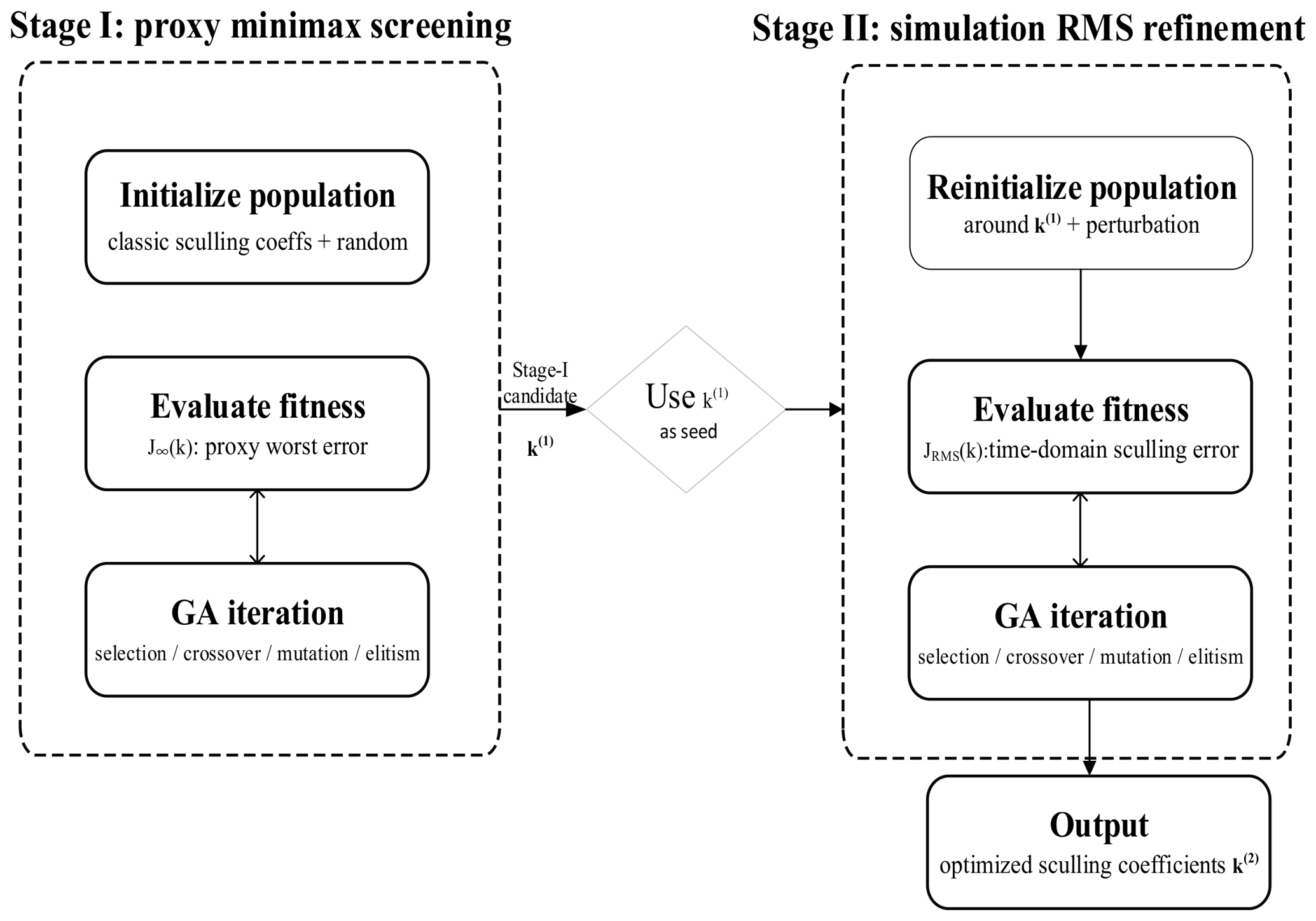
To reduce the computational cost of direct global search based on time-domain simulations, this paper adopts the two-stage design framework shown in Figure 2. In Stage I, an analytical error expansion is used to construct a low-cost proxy model, and a minimax criterion is applied to screen robust candidate coefficients over the entire interval, yielding k⁽¹⁾. In Stage II, k⁽¹⁾ is used as the initial candidate and further refined by multi-condition time-domain simulations with an RMS objective, resulting in the final velocity-specific coefficients k⁽²⁾. Thus, Stage-I proxy minimax provides a robust candidate with a reasonably low-order error structure, whereas Stage-II time-domain RMS refinement directly improves the final performance with respect to the simulated sculling compensation error.

3.2. Proxy-Model-Based Finite-Interval Minimax Design of Six-Sample Coefficients

High-fidelity time-domain simulation is computationally expensive and is therefore not suitable for direct global worst-case optimization over the prescribed interval λ ∈ [0, 1]. To reduce the search cost, a low-cost proxy model is introduced in Stage I to screen candidate six-sample sculling compensation coefficients. Based on the analytical error expansion derived in Section 2, a truncated odd-order proxy error polynomial is constructed, and the corresponding finite-interval minimax optimization problem is formulated.

Let the six-sample sculling compensation coefficient vector be k = [k₁,k₂,k₃,k₄,k₅]^T. According to the derivation in Equations (23)–(25), the six-sample sculling compensation error can be expressed as an odd-order series about λ = 0.

The number of retained terms is determined by the coefficient degrees of freedom and the classical cancellation structure. In the compact six-sample formulation, the design vector contains five independent coefficients, denoted by k₁, k₂, k₃, k₄, and k₅. Correspondingly, the classical six-sample sculling coefficients are obtained by canceling the first five odd-order error coefficients, i.e., c₃, c₅, c₇, c₉, and c₁₁. Therefore, retaining the first five odd-order terms in the Stage-I proxy model preserves all low-order error components that are directly associated with the available coefficient degrees of freedom. Retaining fewer terms would not fully represent the classical six-sample cancellation conditions, whereas retaining additional higher-order terms would introduce components that cannot be independently canceled by the five coefficients and may make the truncated proxy more sensitive to higher-order approximation errors. For this reason, the higher-order finite-step effects are not forced into the Stage-I proxy model but are instead handled by the Stage-II time-domain RMS refinement. Accordingly, the Stage-I proxy error model is defined as follows:

$${\Phi }_p(\lambda ;k)=c_3{\lambda }^3+c_5{\lambda }^5+c_7{\lambda }^7+c_9{\lambda }^9+c_{11}{\lambda }^{11}$$

(29)

where λ = ΩΔT, and c₃, c₅, c₇, c₉, and c₁₁ denote the retained odd-order coefficients in the error expansion derived in Section 2. This proxy model provides a compact approximation of the dominant error trend and is suitable for the initial robust screening over the prescribed finite interval.

To suppress possible error peaks over λ ∈ [0, 1] and improve the performance uniformity over the whole working interval, the Stage-I objective function is defined as the worst-case absolute value of the proxy error over the interval:

$$J_{\infty }(k)={\max }_{\lambda \in [0,1]}\left|{\Phi }_p(\lambda ;k)\right|$$

(30)

The coefficient feasibility constraints used in the numerical optimization are imposed as:

$$0\le k_i\le 1, i=1,2,\dots ,5$$

(31)

Accordingly, the Stage-I optimization problem can be formulated as:

$$k^{(1)}=\arg {\min }_k{J}_{\infty }(k)$$

(32)

This optimization minimizes the worst-case proxy error over the finite working interval and suppresses potential error peaks at a low computational cost, thereby screening candidate coefficients with improved interval-wide robustness. It should be noted that the Stage-I result is mainly used to generate a robust candidate under the proxy error metric. Its role is to provide a reasonable and robust initial solution for the subsequent Stage-II time-domain RMS refinement. The final coefficient performance still needs to be further evaluated and corrected using a more realistic time-domain error metric.

3.3. Stage-II Time-Domain RMS Refinement Based on Multi-Condition Simulations

The Stage-I proxy minimax design can obtain candidate coefficients with finite-interval robustness at a relatively low computational cost. However, the truncated odd-order proxy model mainly reflects the low-order error structure near λ = 0 and cannot fully represent the actual time-domain error in velocity updating caused by discrete sampling, body-frame rotation, and angular-increment–velocity-increment coupling. In particular, as λ increases within the finite working interval, higher-order error terms, different initial phases, and different subsample aggregation bases may all affect the final compensation accuracy. Therefore, after obtaining the Stage-I candidate coefficients, this paper introduces multi-condition time-domain simulations and uses the RMS sculling compensation error as the Stage-II objective to further refine the six-sample coefficients.

Let the six-sample coefficient vector to be optimized be k = [k₁,k₂,k₃,k₄,k₅]^T. For a given condition c_mn = (λ_m,t_0,n), where λ_m = Ω_mΔT and t_0,n is the initial phase, high-rate angular and velocity increments within one velocity-update interval are first generated according to the sculling motion model defined in Section 2. These high-rate increments are then aggregated into six subsample angular increments and six subsample velocity increments, denoted by Δθ_i and Δv_i, i = 1, …, 6, respectively. For a given coefficient vector k, the sculling compensation estimate obtained by the six-sample algorithm is written as:

$$\delta v_{\mathrm{est}}(k;c_{mn},b)={\displaystyle {\displaystyle \sum _{s=1}^5}{k}_s}{\displaystyle {\displaystyle \sum _{i=1}^{6-s}}\left(\Delta {\theta }_i\times \Delta v_{i+s}+\Delta v_i\times \Delta {\theta }_{i+s}\right)}$$

(33)

where s denotes the spacing order between two subsamples, and b denotes the starting index for subsample aggregation. Equation (33) is consistent with the compact six-sample structure established in Section 2, except that the angular and velocity increments are directly generated from time-domain simulations rather than from the analytical series expansion.

To evaluate the actual error of the compensation term in Equation (33), a high-accuracy reference compensation term is required. In this paper, oversampled integration is used to compute the reference velocity increment over the same velocity-update interval, while accounting for the influence of body-frame rotation on the specific-force integration. Let Δv_ref denote the reference velocity increment obtained by oversampled integration, and let Δθ_m and Δv_m denote the total angular increment and total velocity increment over the current velocity-update interval, respectively. The reference sculling compensation term is then defined as:

$$\delta v_{\mathrm{ref}}(c_{mn},b)=\Delta v_{\mathrm{ref}}(c_{mn},b)-\Delta v_m(c_{mn},b)-{\displaystyle \frac{1}{2}}\Delta {\theta }_m(c_{mn},b)\times \Delta v_m(c_{mn},b)$$

(34)

Equation (34) represents the higher-order coupled compensation component after subtracting the direct velocity increment and the first-order rotational compensation term from the reference velocity increment. This quantity is regarded as the reference value that the six-sample sculling compensation algorithm should approximate under the current condition.

For a given condition, c_mn and starting index b, the six-sample sculling compensation error and its scalar norm are defined as:

$$e_b(k;{\lambda }_m,t_{0,n})=\delta v_{\mathrm{est}}(k;c_{mn},b)-\delta v_{\mathrm{ref}}(c_{mn},b), r_b(k;{\lambda }_m,t_{0,n})={‖e_b(k;{\lambda }_m,t_{0,n})‖}_2$$

(35)

where e_b is the vector error, and r_b is the corresponding Euclidean norm.

To reduce the influence of the subsample aggregation starting position on the evaluation results, a worst-over-base strategy is adopted in Stage II. Specifically, for the same (λ_m,t_0,n), the errors under different candidate starting indices are computed, and the maximum value is used as the conservative error for this condition:

$$r_{\mathrm{wb}}(k;{\lambda }_m,t_{0,n})={\max }_{b\in B}{r}_b(k;{\lambda }_m,t_{0,n})$$

(36)

where B denotes the set of candidate starting indices, and r_wb is the error after worst-over-base aggregation. This treatment prevents the optimized coefficients from being effective only for a fixed sampling base, thereby improving their robustness in discrete implementation.

The Stage-II condition set is constructed by uniformly sampling both λ and the initial phase t₀. Specifically, N_λ samples are taken over λ ∈ [0, 1], and N_t0 initial phases are taken over t₀ ∈ [0, 2π). Based on the conservative error defined in Equation (36), the Stage-II RMS objective function is defined as:

$$J_{\mathrm{RMS}}(k)=\sqrt{{\displaystyle \frac{1}{N_{\lambda }{N}_{t0}}}{\displaystyle \sum _{m=1}^{N_{\lambda }}{\displaystyle \sum _{n=1}^{N_{t0}}{\left[r_{\mathrm{wb}}(k;{\lambda }_m,t_{0,n})\right]}^2}}}$$

(37)

To evaluate the performance under the most adverse condition, the global worst-case error is also defined as:

$$J_{\max }(k)={\max }_{\begin{array}{c}1\le m\le N_{\lambda }\\ 1\le n\le N_{t0}\end{array}}{r}_{\mathrm{wb}}(k;{\lambda }_m,t_{0,n})$$

(38)

Therefore, the Stage-II refinement problem can be formulated as

$${\min }_k{J}_{\mathrm{RMS}}(k), 0\le k_i\le 1, i=1,2,\dots ,5$$

(39)

Unlike Stage I, Stage II no longer optimizes the truncated proxy polynomial but directly minimizes the multi-condition time-domain simulation error. The role of Stage I is to provide candidate coefficients with a reasonably low-order error structure, whereas Stage II further refines these coefficients according to the actual velocity-update error metric. In this way, the six-sample sculling compensation coefficient design is extended from local error cancellation in the small-parameter neighborhood to simulation-based performance optimization over a finite working interval.

The RMS metric is adopted as the primary Stage-II objective because it reflects the overall error level over the complete λ–phase condition set. By contrast, the worst-case metric is more sensitive to isolated extreme conditions and may bias the search toward a small number of peak-error samples if it is used as the sole objective. Therefore, RMS minimization is used for coefficient refinement, while the global worst-case error is retained as an independent robustness indicator. This formulation allows the optimized coefficients to be evaluated from both the overall-error and peak-error perspectives.

3.4. Genetic Algorithm Solver and Two-Stage Implementation Details

To solve the finite-interval robust coefficient design problems formulated in Section 3.2 and Section 3.3, a genetic algorithm (GA) is adopted as the numerical optimizer. It should be emphasized that this paper does not aim to propose new GA operators. Instead, the focus is to reformulate the six-sample sculling compensation coefficient design from local small-parameter error cancellation to a two-stage robust optimization problem over a finite working interval. Therefore, GA is used mainly as a unified global-search and refinement tool [25,26].

3.4.1. Individual Encoding and Constraint Handling

For the six-sample sculling compensation algorithm, the design variables are the five compensation coefficients grouped by subsample spacing, namely k = [k₁,k₂,k₃,k₄,k₅]^T. Accordingly, each GA individual is encoded as a five-dimensional real-valued vector, directly representing one candidate coefficient set. Following the settings in Section 3.2 and Section 3.3, all coefficient components are constrained within the same bounded interval, 0 ≤ k_i ≤ 1, i = 1, …, 5.

During initialization and genetic operations, if crossover or mutation generates a coefficient outside this interval, boundary clipping is applied to project it back into [0, 1]. This treatment ensures the feasibility of all candidate coefficients and makes Stage I and Stage II share the same search space.

In Stage I, the initial population consists of random individuals and the classical six-sample coefficient vector. The classical coefficients are injected as one initial individual so that the search starts from a population containing the traditional local-optimal structure. The remaining individuals are generated uniformly at random within [0, 1]⁵. In Stage II, the population is initialized around the Stage-I candidate coefficients: the Stage-I best individual is retained as an elite individual, while the remaining individuals are generated by applying small Gaussian perturbations around this candidate. This strategy allows Stage II to start from a region with a reasonably low-order error structure and further refines the coefficients with respect to the time-domain RMS objective.

3.4.2. Fitness Functions and Stage Switching

The two optimization stages use different fitness functions. In Stage I, the proxy minimax metric defined in Section 3.2 is used as the fitness function, i.e., F₁(k) = J_∞(k). This stage aims to suppress the peak value of the proxy error over the finite interval and obtain candidate coefficients with improved interval-wide robustness.

In Stage II, the multi-condition time-domain RMS metric defined in Section 3.3 is used as the fitness function, i.e., F₂(k) = J_RMS(k). This metric aggregates the simulated sculling compensation errors over different values of λ, initial phase t₀, and starting index b. Unlike Stage I, Stage II does not rely on the truncated proxy polynomial but directly optimizes the sculling compensation error in velocity updating.

Therefore, the two-stage implementation can be summarized as:

$$k^{(1)}=\arg {\min }_{k\in {[0,1]}^5}{J}_{\infty }(k), k^{(2)}=\arg {\min }_{k\in {[0,1]}^5}{J}_{\mathrm{RMS}}(k)$$

(40)

where k⁽¹⁾ denotes the proxy-robust candidate coefficients obtained in Stage I, and k⁽²⁾ denotes the final refined coefficients obtained in Stage II. In implementation, the Stage-II population is initialized around k⁽¹⁾ rather than being completely randomly initialized. This preserves the low-order error structure provided by Stage I while allowing time-domain simulations to further correct the discrepancy between the proxy model and the actual velocity-update error.

The initial population in Stage II is generated as:

$$k_j^{(0)}=\mathrm{clip}\left(k^{(1)}+{\eta }_j, 0, 1\right), {\eta }_j~\mathcal{N}(0,{\sigma }_{\mathrm{init}}^{2}I)$$

(41)

where clip(·) denotes boundary clipping, and σ_init is the standard deviation of the initialization perturbation in Stage II. For the elite individual, k₁⁽⁰⁾ is directly set to k⁽¹⁾, ensuring that the Stage-I candidate solution is not lost during Stage-II initialization.

3.4.3. Genetic Operators

The same basic genetic operators are used in both stages, including tournament selection, real-valued crossover, Gaussian mutation, and elitism. Tournament selection is used to choose parent individuals, where the individual with the smallest fitness value among several randomly sampled candidates is selected as a parent. Since both Stage I and Stage II are formulated as minimization problems, a smaller fitness value indicates better performance.

For crossover, a real-valued linear blending strategy is adopted to generate offspring between two parent coefficient vectors. Mutation is implemented by applying Gaussian perturbations to each gene component with a prescribed mutation probability, followed by boundary clipping to ensure that all coefficients remain within [0, 1]. A larger mutation strength is used in Stage I to maintain global search capability, whereas a smaller mutation strength is used in Stage II to refine the solution locally around the Stage-I candidate coefficients.

Finally, elitism is used to prevent the current best individual from being lost during genetic operations. In each generation, the individual with the smallest fitness value is directly copied to the next generation, ensuring non-degradation of the best fitness and improving the stability of the optimization process.

3.4.4. Implementation Parameters

A unified set of GA parameters is used for the two-stage coefficient optimization. The main hyperparameters for the GA and the Stage-II simulation-based refinement are summarized in

Table 1. Hyperparameters for genetic algorithms and two-stage optimization.

Parameter	Symbol/Name	Value
Gene dimension	d	5
Gene range	$k_i\in \left[\cdot \right]$	clamped to [0, 1]
Population size	population_size	80
Stage-I max generations	generations1	300
Stage-II max generations	generations2	300
Crossover probability	pc	0.9
Tournament size	kt	3
Mutation probability	pm	0.1
Stage-I mutation std	σmut	0.2
Stage-II initialization perturbation std	refine_init_sigma	0.05
Stage-II mutation std	σref	0.02
Stage-I grid points (for λ ∈ [0, 1])	Nx	200 (uniform over [0, 1])
Stage-II λ samples	Nλ	30 (uniform over [0, 1])
Initial phase samples	Nt0	8 (uniform over [0, 2π), i.e., 0, π/4, …, 7π/4)
Velocity update interval	T	0.1 s (10 Hz)
High-rate step	dt	h/12 = 0.008333 s (120 Hz)
High-rate samples per update	Nh	12
Number of subsamples	Nsub	6
Subsample interval	ΔT	T/6 = 0.016667 s
Oversampling factor for truth integration	oversample	100

.

Under these settings, Stage I performs a minimax search on the proxy-error grid over λ ∈ [0, 1], whereas Stage II directly minimizes the RMS error over the multi-condition time-domain simulation set. In Stage II, N_λ = 30 and N_t0 = 8 are used, resulting in 30 × 8 = 240 basic evaluation conditions. With the worst-over-base aggregation, the errors associated with different subsample aggregation starting indices are also considered for each basic condition, making the objective more conservative.

It should be emphasized that Stage I and Stage II play different roles. Stage I generates candidate coefficients with finite-interval robustness based on the analytical error structure, whereas Stage II further refines these candidates using time-domain simulation errors. Therefore, even if the Stage-I result is close to the classical six-sample coefficients, it still provides a structurally reasonable initial solution for Stage-II refinement. The final coefficient performance is evaluated using the RMS and worst-case error metrics in the following sections.

3.5. Two-Stage Optimization Results and Preliminary Validation

To verify the effectiveness of the proposed two-stage coefficient design method, this section provides a preliminary comparison of different six-sample sculling compensation coefficients using the multi-condition time-domain simulation framework defined in Section 3.3. The evaluation set consists of 30 uniformly sampled points over λ ∈ [0, 1] and eight uniformly sampled initial phases over t₀ ∈ [0, 2π), resulting in 240 basic conditions. For each (λ,t₀) pair, the worst-over-base strategy is used to conservatively aggregate the errors associated with different subsample aggregation starting indices. The evaluation metrics include the global RMS error J_RMS and the global worst-case error J_max.

Four coefficient sets are compared: the classical six-sample coefficients, the Stage-I coefficients obtained by proxy minimax optimization, the attitude-transfer coefficients directly transferred from the optimized coefficients in the attitude-updating problem, and the Stage-II coefficients refined by the time-domain RMS objective for velocity updating.

Table 2. Six-sample sculling compensation coefficient vectors.

Coefficient Set	k1	k2	k3	k4	k5
Classic	0.683853	0.423918	0.526407	0.493290	0.501082
Stage I	0.683853	0.423918	0.526407	0.493290	0.501082
Attitude transfer	0.559690	0.311798	0.363498	0.373433	0.394812
Stage II	0.587602	0.206307	0.263713	0.208943	0.917109

lists the four coefficient vectors.

As shown in Table 2, under the current proxy minimax setting, the Stage-I coefficients are identical to the classical six-sample coefficients. This indicates that the Stage-I optimization preserves the low-order error structure of the classical Taylor-cancellation coefficients in the present sculling proxy model. In contrast, both the attitude-transfer and Stage-II coefficients deviate noticeably from the classical coefficients. The attitude-transfer coefficients are obtained by directly transferring the optimized coefficients from the attitude-updating problem to the velocity sculling compensation structure, whereas the Stage-II coefficients are velocity-specific coefficients refined under the time-domain RMS error metric.

To further compare the actual compensation performance of different coefficient schemes,

Table 3. Preliminary validation results for different six-sample sculling compensation coefficients.

Coefficient Set	JRMS	Jmax	Valid Cases	RMS Gain vs. Classic	Worst Gain vs. Classic
Classic	0.035719	0.069290	240	1.000×	1.000×
Stage I	0.035719	0.069290	240	1.000×	1.000×
Attitude transfer	0.032010	0.062260	240	1.116×	1.113×
Stage II	0.031238	0.059449	240	1.143×	1.166×

reports the global error metrics under the same evaluation conditions. Both RMS gain and Worst gain are calculated relative to the classical coefficients; larger values indicate greater error reduction with respect to the classical baseline.

As shown in Table 3, the Stage-I coefficients give almost the same J_RMS and J_max as the classical coefficients, which is consistent with the coefficient vectors in Table 2. This indicates that, under the present proxy minimax setting, Stage I preserves the low-order Taylor-cancellation structure of the classical six-sample coefficients. Therefore, the Stage-I result can be regarded as a confirmation of the classical baseline under the proxy robustness criterion, and it provides a structurally reasonable initial solution for subsequent refinement.

Compared with the classical coefficients, the attitude-transfer coefficients already reduce both the global RMS and worst-case errors, suggesting that optimized coning compensation coefficients have partial transferability to velocity sculling compensation. The velocity-specific Stage-II coefficients further achieve the lowest errors among the four schemes, with RMS and worst-case gains of 1.143 and 1.166, respectively. This shows that although attitude-transfer coefficients provide a useful reference, velocity updating still benefits from coefficient redesign based on its own time-domain error metric.

It should be noted that Table 3 reports global aggregate metrics over the whole condition set. Since Stage II is optimized using a multi-condition RMS objective, its advantage is reflected mainly in the overall RMS and worst-case performance, rather than in strict pointwise superiority at every λ sample. Section 4 therefore further analyzes the curve-level metrics J_RMS(λ) and J_max(λ) under more stringent protocols, different motion cases, and ablation settings.

In summary, these preliminary results verify the effectiveness of the proposed two-stage design framework for velocity updating. Stage I preserves the classical low-order error structure, while Stage II refines the coefficients using time-domain simulations and improves the global RMS and worst-case error metrics.

3.6. Summary of the Proposed Design Method

This section establishes a two-stage finite-interval robust design method for six-sample sculling compensation coefficients. Based on the analytical error expansion derived in Section 2, a truncated odd-order proxy error model was constructed, and the classical local Taylor-cancellation design was extended to a finite-interval minimax problem over λ ∈ [0, 1]. This Stage-I proxy minimax step was used to generate candidate coefficients with interval-wide robustness.

A Stage-II time-domain RMS refinement was then introduced to further optimize the candidate coefficients using multi-condition simulations over different λ, initial phases, and subsample aggregation bases. The resulting objective directly reflects the simulated sculling compensation error in velocity updating and therefore provides a more realistic performance metric than the truncated proxy model.

The preliminary results show that, under the current proxy minimax setting, the Stage-I coefficients coincide with the classical six-sample coefficients, confirming the strong baseline robustness of the classical Taylor-cancellation structure. The attitude-transfer coefficients reduce the velocity-update error to some extent, indicating structural similarity between coning and sculling compensation. However, the velocity-specific Stage-II coefficients achieve better global RMS and worst-case performance, demonstrating the necessity of coefficient redesign based on the time-domain error metric of velocity updating.

Overall, this section completes the formulation and preliminary validation of the proposed finite-interval robust coefficient design method. The next section further evaluates the classical coefficients, attitude-transfer coefficients, and velocity-specific optimized coefficients under more stringent protocols, different motion cases, and ablation settings.

4. Numerical Experiments and Analysis

This section numerically evaluates the proposed finite-interval robust coefficient design method for six-sample sculling compensation. Different from Section 3, which focuses on method formulation and preliminary validation, this section further compares the classical coefficients, Stage-I coefficients, attitude-transfer coefficients, velocity-specific Stage-II coefficients, and random coefficients under stringent evaluation protocols and complex velocity-updating inputs. The experiments are designed as UAV-oriented algorithm-level validation rather than full mission-level flight simulation. For onboard UAV strapdown INS, rapid attitude changes, sustained acceleration, turning motion, rotor-induced vibration, and GNSS-degraded operation can produce coupled angular-rate and specific-force inputs in the velocity-updating process. Therefore, representative angular-rate and specific-force excitations are constructed to isolate and evaluate the sculling compensation error over the finite working interval λ ∈ [0, 1]. This setting allows different coefficient schemes to be compared under controlled yet UAV-relevant motion conditions.

This section focuses on three aspects. First, the global RMS and worst-case error reductions achieved by the velocity-specific Stage-II coefficients are examined under conservative evaluation conditions with dense phase sampling and uncertain subsample aggregation bases. Second, the effectiveness of attitude-transfer coefficients in velocity updating is assessed, and their performance is compared with that of the velocity-specific redesigned coefficients. Third, the robustness of the optimized coefficients is further evaluated when the nominal single-frequency sculling model is extended to include specific-force bias, angular-rate bias, and double-frequency components.

Section 4.1 presents the unified experimental setup. Section 4.2 evaluates the coefficient schemes under the standard single-frequency sculling motion using a stringent protocol. Section 4.3 further investigates their generalization performance under three complex sculling motions. Section 4.4 provides ablation analysis and numerical reproducibility checks.

4.1. Unified Experimental Settings

Unless otherwise specified, all experiments in this section use the same velocity-updating simulation settings. The velocity-update interval is set to T = 0.1 s. Each update interval contains N_high = 12 high-rate samples, and the number of subsamples used by the six-sample sculling compensation algorithm is N_sub = 6. The reference sculling compensation term is obtained by oversampled time-domain integration with an oversampling factor of 100. The dimensionless parameter is defined as λ = ΩΔT, where Ω is the characteristic angular frequency and ΔT = T/6 is the subsample interval of the six-sample algorithm.

The experiments focus on the sculling compensation error caused by the coupling between angular and velocity increments in velocity updating. This relatively isolated evaluation makes it possible to directly compare different six-sample coefficient schemes while avoiding interference from other error sources in a complete inertial velocity-update chain.

4.1.1. Coefficient Schemes for Comparison

Five types of six-sample sculling compensation coefficients are compared in this section.

The first set is the classical six-sample sculling compensation coefficients, denoted by k_cls. These coefficients are derived from a small-parameter Taylor expansion and leading-error-term cancellation and are used as the reference baseline for all improvement ratios.

The second set is the Stage-I coefficients, denoted by k⁽¹⁾. These coefficients are obtained by finite-interval proxy minimax optimization. Under the present proxy model, k⁽¹⁾ coincides with k_cls, indicating that the classical Taylor-cancellation coefficients already form a strong, robust baseline in the low-order proxy model.

The third set is the attitude-transfer coefficients, denoted by k_att. These coefficients are transferred from the optimized coning compensation coefficients in the attitude-updating problem and directly applied to the six-sample sculling compensation structure in velocity updating. This set is included to examine the structural similarity and transferability between attitude coning compensation and velocity sculling compensation.

The fourth set is the velocity-specific Stage-II coefficients, denoted by k⁽²⁾. These coefficients are obtained by multi-condition time-domain RMS refinement and represent the final velocity-updating coefficients proposed in this paper. Unlike the classical and Stage-I coefficients, k⁽²⁾ is directly optimized with respect to the finite-interval time-domain sculling compensation error.

The fifth set is the random coefficients, denoted by k_rand. They are sampled uniformly from the same constraint space [0, 1]⁵ and are used as non-optimized references. Since individual random samples may occasionally produce favorable results, this paper reports the median performance and the min–max range over multiple random samples rather than over-interpreting any single random coefficient vector.

4.1.2. Evaluation Procedure and Metrics

For a given coefficient vector k, high-rate angular and velocity increments are first generated within one velocity-update interval under the specified motion model. These high-rate increments are then aggregated into six subsample angular increments and six subsample velocity increments, which are substituted into the six-sample sculling compensation formula to obtain the compensation estimate δv_est. Meanwhile, the reference compensation term δv_ref is computed by oversampled time-domain integration.

For each condition c = (λ,t₀), the sculling compensation error is defined as the difference between the estimated and reference compensation terms, and its Euclidean norm is used as the scalar error. For each value of λ, the scalar errors over different initial phases t₀ are aggregated to obtain the curve-level metrics RMS(λ) and Worst(λ). The global metrics RMS_all and Worst_all are then obtained by further aggregation over the whole condition set.

When the uncertainty of the subsample aggregation starting position is considered, the worst-over-base strategy is adopted. Specifically, for the same (λ,t₀), the errors under different starting indices b are computed, and the maximum value is used as the conservative error for that condition. When a fixed starting index is used, no worst-over-base aggregation is applied.

4.1.3. Representative Motion Cases

This section considers one standard sculling case and three complex sculling cases. The standard case provides the basic finite-interval evaluation benchmark, whereas the complex cases are used to examine the stability of different coefficient schemes when the velocity-updating inputs deviate from the nominal single-frequency model.

The standard single-frequency sculling case follows the basic model defined in Section 2, where the angular rate oscillates along the first body-frame axis, and the specific force oscillates along the second body-frame axis. This model directly excites the angular-increment–velocity-increment coupling in sculling compensation and serves as the basic benchmark for comparing different six-sample coefficients.

The constant-specific-force-biased sculling case adds a constant component to the specific-force input of the standard model. It is used to approximate oscillatory specific-force inputs under sustained acceleration, thrust bias, or slowly varying linear maneuvers, and mainly examines the influence of a nonzero mean specific-force background.

The constant-angular-rate-biased sculling case adds a constant angular-rate component about the third body-frame axis. It is used to approximate velocity updating under turning, sustained yaw motion, or background attitude maneuvers, and mainly examines the influence of background angular motion on angular-increment–velocity-increment coupling errors.

The double-frequency sculling case adds second-harmonic components to both the angular-rate and specific-force inputs. It is used to represent more complex coupled inputs caused by rotor vibration, structural vibration, or multi-frequency maneuvers, and tests whether the optimized coefficients remain effective beyond the nominal single-frequency sculling condition.

4.1.4. UAV-Relevant Interpretation of Motion Cases

The motion cases used in this study are selected to represent typical excitation sources encountered in onboard UAV strapdown INS velocity updating. The standard single-frequency sculling case provides a canonical benchmark for angular-rate–specific-force coupling. The constant-specific-force case represents sustained thrust, acceleration, or slowly varying translational maneuver backgrounds. The constant-angular-rate case corresponds to turning, yawing, or sustained attitude maneuvers of UAV platforms. The double-frequency sculling case is used to approximate additional harmonic components caused by rotor vibration, structural vibration, or multi-frequency maneuvering. Therefore, these controlled motion cases provide UAV-relevant algorithm-level validation by focusing on the error mechanisms that affect onboard inertial velocity updating.

4.1.5. Evaluation Protocols

To balance conservativeness and computational cost, two evaluation protocols are used in this section.

Protocol A: stringent single-frequency sculling. This protocol is used in Section 4.2. The motion model is the standard single-frequency sculling case. The parameter λ is uniformly sampled over [0, 1] with N_λ = 30, and the initial phase t₀ is uniformly sampled over [0, 2π) with N_t0 = 64. For each (λ,t₀) pair, the worst-over-base strategy is applied. This protocol is used to evaluate the global robustness of different coefficient schemes under dense phase sampling and uncertain subsample aggregation bases.

Protocol B: complex sculling motions. This protocol is used in Section 4.3. To reduce the computational cost of evaluating multiple motion cases, the number of initial phase samples is set to N_t0 = 8, and the subsample aggregation starting index is fixed at b = 0. The complex motions include constant-specific-force-biased sculling, constant-angular-rate-biased sculling, and double-frequency sculling. This protocol is used to examine whether the velocity-specific Stage-II coefficients maintain stable error reduction under complex velocity-updating inputs involving constant components and multi-frequency excitations.

The main differences and common settings of the two protocols are summarized in

Table 4. Experimental settings and evaluation protocols in Section 4.

Setting	Protocol A: Stringent Single-Frequency Sculling	Protocol B: Complex Sculling Motions
Purpose	Conservative finite-interval evaluation	Generalization validation under complex velocity-updating inputs
Corresponding section	Section 4.2	Section 4.3
Motion model	Standard single-frequency sculling	Constant-specific-force-biased sculling, constant-angular-rate-biased sculling, and double-frequency sculling
λ grid	λ ∈ [0, 1], Nλ = 30	Same as Protocol A
Initial phase samples	Nt0 = 64	Nt0 = 8
Initial phase range	t0 ∈ [0, 2π), uniformly sampled	Same as Protocol A
Base strategy	Worst-over-base	Fixed b = 0
Coefficient schemes	Classic/Stage I/attitude transfer/Stage II/RAND	Same as Protocol A
Random coefficient sampling	Krand~U ([0, 1]5)	Same as Protocol A
Number of random samples	Krand = 50	Krand = 20
Random seed	20,260,305	20,260,305
Reported metrics	RMS(λ), Worst(λ), RMSall, Worstall	Same as Protocol A

.

4.1.6. Random Baseline and Computational Environment

Random coefficient vectors are independently sampled from the uniform distribution over [0, 1]⁵, consistent with the coefficient constraints used in the genetic algorithm. No additional feasibility filtering is applied. For Protocol A, the number of random samples is set to K_rand = 50; for Protocol B, it is set to K_rand = 20. The random-baseline results are reported using the median value and the min–max range. In the curve plots, the random baseline is represented by the median curve and the min–max envelope.

All randomized experiments use the fixed random seed 20,260,305 to ensure reproducibility. All numerical experiments are performed on a 64-bit Windows computer equipped with an Intel Core i5-9300H CPU and 16 GB RAM. The program is implemented in C++ and compiled using Visual Studio 2015. The simulation outputs are stored as CSV files and then processed offline to generate the tables and figures.

4.2. Numerical Validation Under Stringent Single-Frequency Sculling Conditions

4.2.1. Setup for Stringent Single-Frequency Sculling

This section uses Protocol A in Table 4 to conservatively evaluate the performance of different six-sample sculling compensation coefficients under standard single-frequency sculling motion. This protocol uses dense initial-phase sampling and accounts for the uncertainty of the subsample aggregation starting position, thereby providing a stringent test of the overall robustness of different coefficient schemes over the finite interval λ ∈ [0, 1].

The standard single-frequency sculling motion is defined as:

$${\omega }_b(t)=\left[\begin{array}{c}B\Omega \cos (\Omega t+t_0)\\ 0\\ 0\end{array}\right], f_b(t)=\left[\begin{array}{c}0\\ C\sin (\Omega t+t_0)\\ 0\end{array}\right]$$

where Ω is the characteristic angular frequency, B and C are the amplitude parameters of the angular-rate and specific-force inputs, respectively, and t₀ is the initial phase. The dimensionless parameter is defined as λ = ΩΔT, and 30 uniformly distributed samples are taken over [0, 1]. The initial phase t₀ is uniformly sampled over [0, 2π) with N_t0 = 64, resulting in 30 × 64 = 1920 basic conditions. For each (λ,t₀) pair, the worst-over-base strategy is applied to conservatively aggregate the errors associated with different subsample aggregation starting indices.

This section compares five coefficient schemes: classic, Stage I, attitude transfer, Stage II, and RAND. The RAND baseline consists of K_rand = 50 random coefficient vectors and is reported using the median value and the min–max range.

Table 5. Global performance of different coefficient schemes under Protocol A.

Coefficient Scheme	RMSall	Worstall	RMS Gain vs. Classic	Worst Gain vs. Classic
classic	0.035744	0.069290	1.000×	1.000×
Stage I	0.035744	0.069290	1.000×	1.000×
attitude transfer	0.032029	0.062260	1.116×	1.113×
Stage II	0.031252	0.059449	1.144×	1.166×
RAND, K = 50	0.034749 [0.031321, 0.052547]	0.066838 [0.056910, 0.091228]	1.029×	1.037×

summarizes the global error metrics of different coefficient schemes under Protocol A.

4.2.2. Results

As shown in Table 5, the Stage-I coefficients give identical global errors to the classic coefficients, confirming that the proxy minimax result preserves the classical low-order Taylor-cancellation structure. The attitude-transfer coefficients reduce both RMS_all and Worst_all, indicating that optimized coning compensation coefficients have partial transferability to velocity sculling compensation.

The velocity-specific Stage-II coefficients achieve the lowest errors among the deterministic schemes. Compared with the classic coefficients, Stage II provides gains of 1.144 and 1.166 in RMS_all and Worst_all, respectively. The RAND median is slightly better than the classic baseline but remains weaker than Stage II. Although some individual random samples may occasionally approach the Stage-II error level, the random coefficients lack a deterministic design basis and show noticeable variability. Therefore, RAND is used only as a non-optimized reference range.

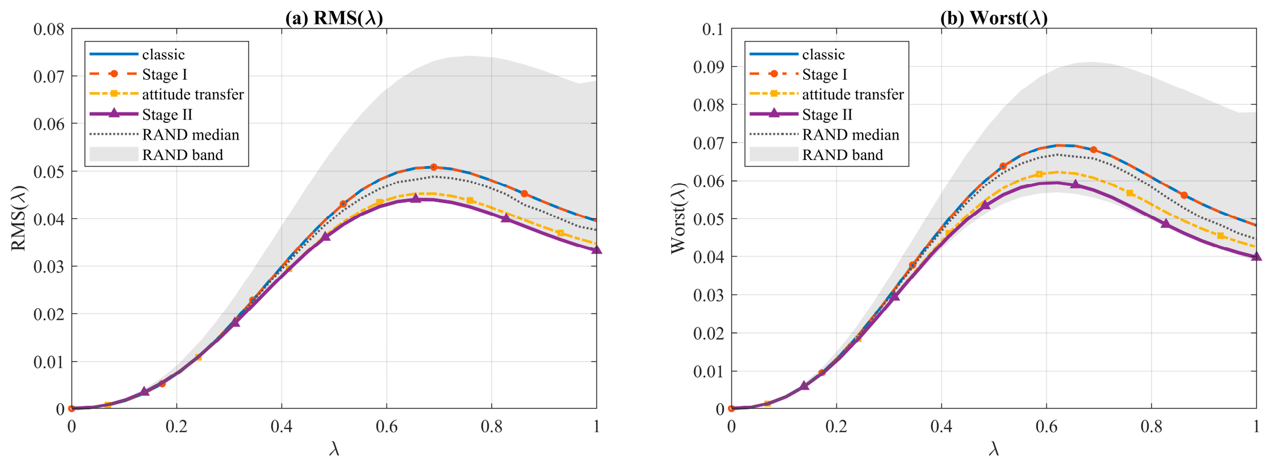
Figure 3 further shows the variation in the curve-level errors with λ. The classic and Stage-I curves almost overlap, which is consistent with the global metrics in Table 5. The attitude-transfer curves are generally below the classic and Stage-I curves, while the Stage-II curves are further reduced, especially in the medium-to-high λ range and near the error peaks.

It should also be noted that Stage II is not strictly superior at every λ sample. In the small-λ region, the classic and Stage-I coefficients remain competitive because they are derived from local Taylor-series cancellation near the small-parameter limit. In contrast, Stage II redistributes the error over the finite interval through time-domain RMS refinement, and its advantage is mainly reflected in the medium-to-high λ region and in the global aggregate metrics.

4.2.3. Analysis of Protocol A Results

Protocol A provides a conservative finite-interval evaluation by combining dense phase sampling with worst-over-base aggregation. Under this protocol, the velocity-specific Stage-II coefficients achieve the best global RMS and worst-case performance among the deterministic schemes, confirming that time-domain RMS refinement improves the overall compensation accuracy under the standard sculling model.

The results also clarify the roles of different coefficient schemes. The classic and Stage-I coefficients represent a strong low-order Taylor-cancellation baseline, the attitude-transfer coefficients indicate partial structural transferability between coning and sculling compensation, and the Stage-II coefficients demonstrate the need for velocity-specific redesign based on angular-increment–velocity-increment coupling errors. Therefore, the proposed Stage-II design does not simply pursue local optimality near λ → 0 but redistributes the error over the finite interval λ ∈ [0, 1] to reduce the global aggregate metrics.

The next section further examines whether this advantage remains stable under complex motions involving specific-force bias, angular-rate bias, and double-frequency sculling.

4.3. Validation Under Complex Sculling Motions

4.3.1. Complex Motion Models and Experimental Setup

To further examine whether the velocity-specific Stage-II coefficients are effective only for the nominal single-frequency sculling model, this section conducts comparative experiments under three complex sculling motions. Unlike the stringent evaluation protocol in Section 4.2, this section adopts Protocol B in Table 4: λ is uniformly sampled over [0, 1] with N_λ = 30, the initial phase t₀ is uniformly sampled over [0, 2π) with N_t0 = 8, and the subsample aggregation starting index is fixed at b = 0. This setting reduces the computational cost while allowing the generalization performance of different coefficient schemes to be evaluated under complex velocity-updating inputs.

The first case is constant-specific-force-biased sculling. A constant component is added to the specific-force input of the standard single-frequency sculling model to approximate oscillatory specific-force inputs under sustained thrust, slowly varying linear maneuvers, or nonzero mean specific-force backgrounds. This case evaluates the error-suppression capability of different six-sample coefficients when the velocity-updating input no longer satisfies the zero-mean single-frequency specific-force assumption. The motion model is:

$${\omega }_b(t)=\left[\begin{array}{c}B\Omega \cos (\Omega t+t_0)\\ 0\\ 0\end{array}\right], f_b(t)=\left[\begin{array}{c}0\\ C\left[\sin (\Omega t+t_0)+{\rho }_f\right]\\ 0\end{array}\right]$$

(42)

where ρ_f is the relative magnitude of the constant specific-force component, and ρ_f = 0.2 is used in this paper.

The second case is constant-angular-rate-biased sculling. A constant angular-rate component about the third body-frame axis is added to the standard single-frequency angular motion to approximate velocity updating under turning, sustained yaw motion, or background attitude maneuvers. This case evaluates the influence of background angular motion on the angular-increment–velocity-increment coupling error. The motion model is:

$${\omega }_b(t)=\left[\begin{array}{c}B\Omega \cos (\Omega t+t_0)\\ 0\\ {\Omega }_s\end{array}\right], f_b(t)=\left[\begin{array}{c}0\\ C\sin (\Omega t+t_0)\\ 0\end{array}\right]$$

(43)

where Ω_s = ρ_sBΩ is the constant angular-rate component added along the third body-frame axis, and ρ_s is its relative magnitude. In this paper, ρ_s = 0.2.

The third case is double-frequency sculling. In this case, second-harmonic components are added simultaneously to the angular-rate and specific-force inputs to represent more complex angular-rate–specific-force coupling caused by rotor vibration, structural vibration, or multi-frequency maneuvers. The motion model is:

$${\omega }_b(t)=\left[\begin{array}{c}B\Omega \left[\cos (\Omega t+t_0)+{\epsilon }_{\mathit{\omega }}\cos (2\Omega t+t_1)\right]\\ 0\\ 0\end{array}\right]$$

(44)

$$f_b(t)=\left[\begin{array}{c}0\\ C\left[\sin (\Omega t+t_0)+{\epsilon }_f\sin (2\Omega t+t_1)\right]\\ 0\end{array}\right]$$

(45)

where ϵ_ω and ϵ_f denote the amplitude ratios of the second-harmonic components in the angular-rate and specific-force inputs, respectively, and t₁ is the phase offset of the second-harmonic component. In this paper, ϵ_ω = ϵ_f = 0.2 and t₁ = π/3.

This section compares the same five coefficient schemes: classic, Stage I, attitude transfer, Stage II, and RAND. The RAND baseline consists of K_rand = 20 random coefficient vectors and is reported using the median value and the min–max range.

4.3.2. Constant-Specific-Force-Biased Sculling Results

Table 6. Global error metrics under constant-specific-force-biased sculling.

Coefficient Scheme	RMSall	Worstall	RMS Gain vs. Classic	Worst Gain vs. Classic
classic	0.033416	0.084949	1.000×	1.000×
Stage I	0.033416	0.084949	1.000×	1.000×
attitude transfer	0.030132	0.076424	1.109×	1.112×
Stage II	0.029868	0.072765	1.119×	1.167×
RAND, K = 20	0.033171 [0.029810, 0.050170]	0.082670 [0.069775, 0.110960]	1.007×	1.028×

reports the global error metrics under constant-specific-force-biased sculling. The Stage-I coefficients give the same results as the classic coefficients, indicating that the classical low-order structure is still preserved in this complex motion case. The attitude-transfer coefficients reduce both RMS_all and Worst_all, while the velocity-specific Stage-II coefficients achieve the lowest errors among the deterministic schemes.

Compared with the classic coefficients, Stage II reduces RMS_all from 0.033416 to 0.029868 and Worst_all from 0.084949 to 0.072765, corresponding to error reductions of approximately 10.62% and 14.34%, respectively. This result indicates that the Stage-II coefficients remain effective even when a nonzero mean specific-force component is introduced into the velocity-updating input.

4.3.3. Constant-Angular-Rate-Biased Sculling Results

Table 7. Global error metrics under constant-angular-rate-biased sculling.

Coefficient Scheme	RMSall	Worstall	RMS Gain vs. Classic	Worst Gain vs. Classic
classic	0.035520	0.073444	1.000×	1.000×
Stage I	0.035520	0.073444	1.000×	1.000×
attitude transfer	0.031672	0.065203	1.122×	1.126×
Stage II	0.031103	0.061565	1.142×	1.193×
RAND, K = 20	0.035324 [0.031182, 0.052501]	0.071566 [0.059422, 0.097894]	1.006×	1.026×

reports the global error metrics under constant-angular-rate-biased sculling. This motion introduces a background angular rate into the standard sculling input and therefore perturbs the angular-increment–velocity-increment coupling structure more directly.

Compared with the classic coefficients, the Stage-II coefficients reduce RMS_all by approximately 12.44% and Worst_all by approximately 16.17%. Among the three complex motion cases, this case shows the most pronounced reduction in the worst-case error. This indicates that the velocity-specific Stage-II coefficients are effective in suppressing the coupling error induced by background angular motion.

4.3.4. Double-Frequency Sculling Results

Table 8. Global error metrics under double-frequency sculling.

Coefficient Scheme	RMSall	Worstall	RMS Gain vs. Classic	Worst Gain vs. Classic
classic	0.033532	0.077313	1.000×	1.000×
Stage I	0.033532	0.077313	1.000×	1.000×
attitude transfer	0.030063	0.070244	1.115×	1.101×
Stage II	0.029675	0.067811	1.130×	1.140×
RAND, K = 20	0.032973 [0.029631, 0.050505]	0.075230 [0.065904, 0.098196]	1.017×	1.028×

reports the global error metrics under double-frequency sculling. In this case, second-harmonic components are introduced into both the angular-rate and specific-force inputs, providing a test of coefficient stability under multi-frequency excitation.

Compared with the classic coefficients, the Stage-II coefficients reduce RMS_all by approximately 11.50% and Worst_all by approximately 12.29%. This result indicates that the velocity-specific Stage-II coefficients remain effective when additional frequency components are present in the velocity-updating inputs.

4.3.5. Curve-Level Error Analysis

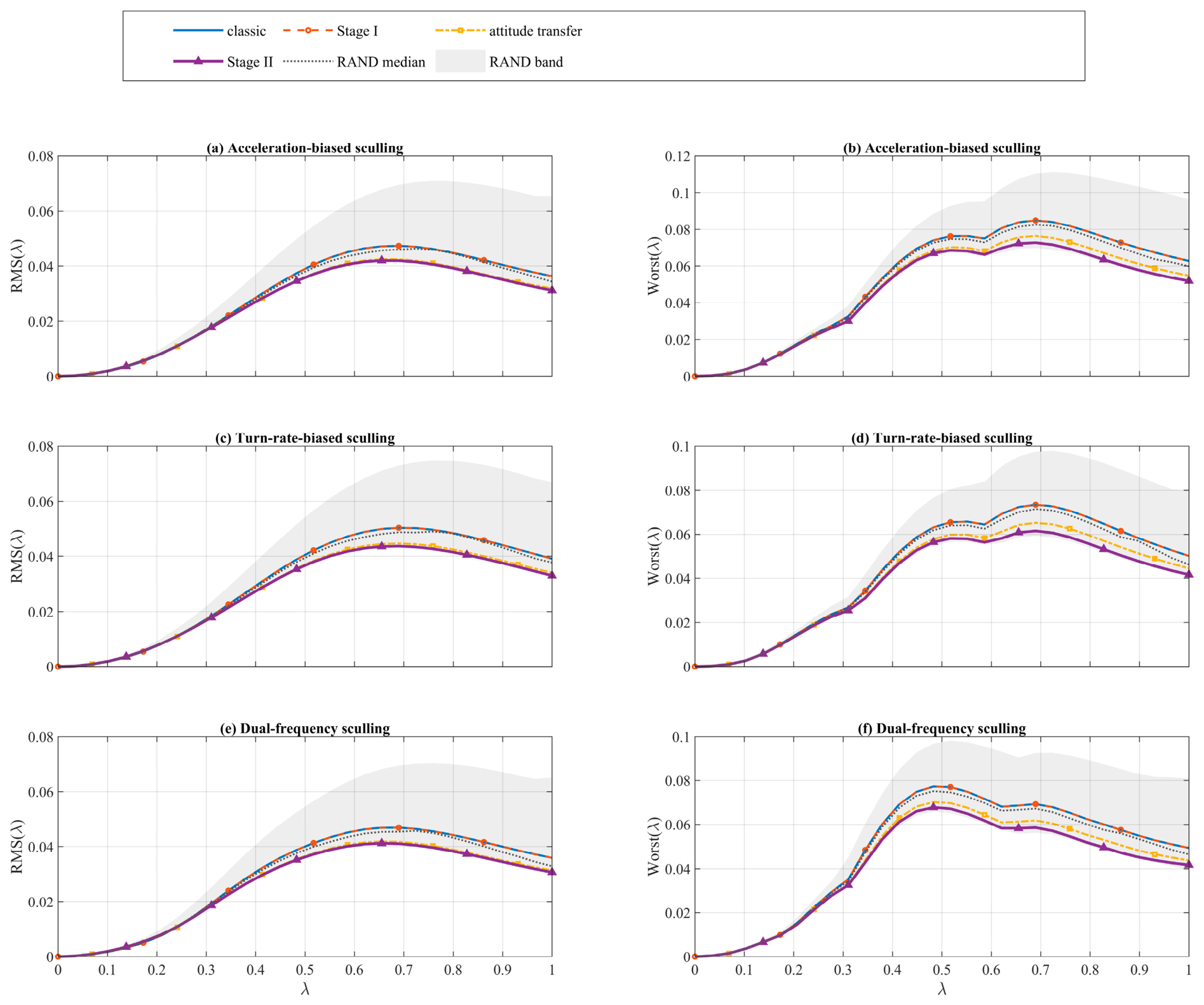
Figure 4 presents the curve-level error metrics under the three complex sculling motions. The left column shows RMS(λ), and the right column shows Worst(λ). The three rows correspond to constant-specific-force-biased sculling, constant-angular-rate-biased sculling, and double-frequency sculling, respectively. The RAND baseline is represented by the median curve and the min–max envelope over 20 random coefficient vectors.

As shown in Figure 4, the overall trends are consistent across the three complex motion cases. The classic and Stage-I curves almost overlap, indicating that the Stage-I proxy minimax result still preserves the classical coefficient structure under complex motions. The attitude-transfer curves are generally lower than the classic and Stage-I curves, confirming that optimized coning compensation coefficients remain partially effective when transferred to velocity sculling compensation.

The Stage-II curves are further reduced in the medium-to-high λ region, especially in the Worst(λ) curves. This indicates that the velocity-specific refinement mainly improves the finite-interval error distribution rather than seeking strict pointwise optimality near the small-λ limit. Consequently, the advantage of Stage II is reflected more clearly in the global RMS_all and Worst_all metrics.

The RAND envelope provides a reference range for non-optimized coefficient vectors. Although some random samples may occasionally approach the optimized results, the median RAND performance is generally weaker than Stage II and lacks a deterministic design basis. Therefore, the random baseline is used only as a non-optimized reference, not as a substitute for coefficient redesign based on the velocity-update error metric.

4.3.6. Analysis of Complex-Motion Results

The results in Table 6, Table 7 and Table 8 and Figure 4 show that the velocity-specific Stage-II coefficients consistently achieve the lowest global errors among the deterministic schemes under all three complex sculling motions. Compared with the classic coefficients, Stage II reduces RMS_all by approximately 10.62–12.44% and Worst_all by 12.29–16.17%. This indicates that the Stage-II coefficients are not only effective for the nominal single-frequency sculling model, but also remain stable under specific-force bias, background angular-rate bias, and double-frequency excitation.

The attitude-transfer coefficients also outperform the classic coefficients in all three complex cases, suggesting a structural connection between multi-sample coning and sculling compensation. However, Stage II further reduces the errors, especially in the worst-case metric. Therefore, attitude-transfer coefficients can provide a useful reference, but they cannot fully replace velocity-specific coefficient redesign based on the time-domain sculling compensation error.

Overall, these results further support the effectiveness of the proposed two-stage design strategy: Stage I preserves the classical low-order structure, while Stage II improves finite-interval performance through velocity-specific time-domain RMS refinement.

4.4. Additional Validation and Ablation Analysis

To further examine the roles of different components in the two-stage coefficient design framework and assess the sensitivity of the main conclusions to numerical settings, this section presents additional validation and ablation analysis. First, a direct RMS optimization scheme is introduced to distinguish the contribution of Stage-I proxy minimax screening from that of Stage-II time-domain RMS refinement. Then, numerical reproducibility checks are conducted by refining the evaluation grid, increasing the reference-integration oversampling factor, and switching the base-index strategy.

4.4.1. Ablation Experiment with Direct RMS Optimization

To evaluate the contribution of the time-domain RMS objective, a direct RMS optimization scheme, denoted as RMS-direct, is constructed. Unlike the proposed two-stage strategy, RMS-direct skips Stage-I proxy minimax screening and directly starts from a randomly initialized population, using the multi-condition time-domain RMS error defined in Section 3 as the fitness function. The resulting coefficients are then compared with classic, Stage I, attitude transfer, and Stage II under the same Protocol A evaluation conditions.

As shown in

Table 9. Ablation results for direct RMS optimization.

Coefficient Scheme	RMSall	Worstall	RMS Gain vs. Classic	Worst Gain vs. Classic
classic	0.035744	0.069290	1.000×	1.000×
Stage I	0.035744	0.069290	1.000×	1.000×
attitude transfer	0.032029	0.062260	1.116×	1.113×
Stage II	0.031252	0.059449	1.144×	1.166×
RMS-direct	0.031252	0.059439	1.144×	1.166×

, Stage I gives identical error metrics to the classic coefficients. This result should not be interpreted as a failure of Stage I, but rather as confirmation that the classical six-sample coefficients already represent the optimal solution for the retained low-order cancellation structure under the current proxy model. In other words, when the optimization objective is restricted to the first five odd-order error terms associated with the five available coefficient degrees of freedom, the proxy minimax design naturally preserves the classical low-order structure. In contrast, both Stage II and RMS-direct clearly outperform classic and attitude transfer, and their global error levels are almost identical. This result indicates that the final numerical improvement mainly comes from changing the objective from local low-order proxy cancellation to multi-condition time-domain RMS refinement. Therefore, the practical role of Stage I is to provide an analytically consistent and reproducible candidate solution, while Stage II is responsible for the main finite-interval performance improvement.

However, the RMS-direct result does not weaken the significance of the two-stage framework. Although direct RMS optimization can reach a similar error level in this experiment, it lacks guidance from the analytical error structure and depends more strongly on random initialization and numerical search. By contrast, the proposed two-stage method first preserves a robust candidate consistent with the classical low-order structure through Stage-I proxy minimax and then refines it using Stage-II time-domain RMS optimization. Therefore, the two-stage framework provides not only low numerical errors but also a more interpretable path from analytical coefficient design to time-domain performance refinement.

The similar performance of RMS-direct and Stage II also suggests that the six-sample sculling coefficient optimization problem may contain multiple low-error coefficient regions rather than a unique optimal coefficient vector. In this case, connecting the final design to the classical analytical structure and finite-interval robustness improves the interpretability and reproducibility of the proposed method.

4.4.2. Numerical Reproducibility Checks

To examine whether the main conclusions depend on specific numerical settings, three reproducibility checks are conducted. First, the evaluation grid is refined from 30 × 64 to 61 × 128 to reduce the influence of discrete sampling. Second, the oversampling factor for reference integration is increased from 100 to 400 to test the sensitivity to reference accuracy. Third, the base strategy is changed from worst-over-base to fixed b = 0 to assess whether the Stage-II advantage depends on conservative base aggregation. Since Stage I remains identical to the classic coefficients in all checks,

Table 10. Numerical reproducibility checks under different evaluation settings.

Evaluation Setting	Coefficient Scheme	RMSall	Worstall	RMS Gain vs. Classic	Worst Gain vs. Classic
Refined grid 61 × 128	classic	0.035868	0.069341	1.000×	1.000×
	attitude transfer	0.032147	0.062244	1.116×	1.114×
	Stage II	0.031374	0.059493	1.143×	1.166×
Oversampling factor 400	classic	0.035748	0.069298	1.000×	1.000×
	attitude transfer	0.032033	0.062267	1.116×	1.113×
	Stage II	0.031255	0.059454	1.144×	1.166×
Fixed base b = 0	classic	0.032164	0.069283	1.000×	1.000×
	attitude transfer	0.028885	0.062228	1.114×	1.113×
	Stage II	0.028615	0.059401	1.124×	1.166×

reports only the results for classic, attitude transfer, and Stage II.

As shown in Table 10, Stage II consistently outperforms both classic and attitude transfer under all three modified settings. With the refined 61 × 128 grid, the RMS and worst-case gains of Stage II remain close to those under Protocol A, indicating that the conclusion is not caused by a coarse λ–phase grid. Increasing the reference-integration oversampling factor to 400 leads to almost unchanged error metrics, showing that the adopted reference-integration accuracy is sufficient for distinguishing the coefficient schemes.

When the fixed base b = 0 is used, the overall RMS errors become lower because the evaluation no longer takes the worst case over different aggregation bases. Nevertheless, Stage II still gives the smallest global errors, and its worst-case gain remains stable. These results confirm that the advantage of Stage II is not sensitive to grid density, reference-integration accuracy, or base-index strategy.

Together with the ablation results in Table 9, these checks indicate that the main numerical improvement comes from the Stage-II time-domain RMS refinement, while Stage I mainly provides an analytically consistent and robust candidate solution. The superiority of Stage II over classic and attitude transfer remains stable under different numerical evaluation settings.

4.5. Sensitivity Analysis and Onboard Implementation

To further examine the numerical reliability and engineering applicability of the proposed coefficient design, several sensitivity and implementation analyses were conducted. These analyses include the sensitivity to GA hyperparameters and random seeds, the sensitivity to the reference-integration oversampling factor, the sensitivity to the prescribed λ interval, an order-of-magnitude propagation analysis of the residual compensation error, and the online implementation complexity. All additional checks are intended to support the robustness and engineering interpretability of the reported Stage-II coefficients.

4.5.1. Sensitivity to GA Hyperparameters and Random Seeds

To examine whether the Stage-II solution depends strongly on GA hyperparameters or random initialization, the Stage-II optimization was repeated under different population sizes, maximum generation numbers, and random seeds. The evaluated results are summarized in

Table 11. Sensitivity of Stage-II optimization to GA settings and random seeds.

Case	Population	Generations	Runs	Mean RMSall	Std RMSall	Mean Worstall	Std Worstall
Default	80	300	3	0.03125158	2.40 × 10−7	0.05944526	7.95 × 10−6
Pop40	40	300	3	0.03125180	4.58 × 10−7	0.05944475	1.27 × 10−5
Pop120	120	300	3	0.03125178	2.26 × 10−7	0.05944207	7.41 × 10−6
Gen150	80	150	3	0.03125484	3.21 × 10−7	0.05949894	2.28 × 10−5
Gen500	80	500	3	0.03125112	1.66 × 10−7	0.05943311	2.11 × 10−6

. For the default setting, three independent runs with different random seeds produced almost identical RMS_all and Worst_all values, indicating that the optimized performance is insensitive to random initialization. Changing the population size from 80 to 40 or 120 also led to negligible changes in the evaluated metrics. When the maximum generation number was reduced from 300 to 150, the error increased slightly, whereas increasing it from 300 to 500 produced only a marginal improvement. These results indicate that the default setting, namely population size 80 and 300 generations, provides a reasonable balance between convergence stability and computational cost. Although the optimized coefficient vectors are not strictly identical in all runs, the resulting RMS_all and Worst_all values remain highly stable, suggesting that the Stage-II optimization contains multiple low-error coefficient regions rather than relying on a single accidental GA solution.

4.5.2. Sensitivity to Reference-Integration Oversampling

The reference sculling compensation term in the main experiments is computed using oversampled time-domain integration. To justify the oversampling factor used in the evaluation, the same coefficient schemes were re-evaluated using 50×, 100×, and 200× reference-integration oversampling factors. The results are shown in

Table 12. Sensitivity of the evaluation results in the reference-integration oversampling factor.

Oversampling Factor	Classic RMSall	Classic Worstall	Stage-II RMSall	Stage-II Worstall	RMS Gain	Worst Gain
50×	0.035739	0.069279	0.031248	0.059442	1.143703	1.165486
100×	0.035744	0.069290	0.031252	0.059449	1.143747	1.165535
200×	0.035747	0.069295	0.031254	0.059452	1.143770	1.165560

. The evaluation metrics are almost unchanged when the oversampling factor varies from 50× to 200×. Compared with the 100× setting, the relative changes in the Stage-II RMS_all and Worst_all values are below 0.012% for 50× and below 0.006% for 200×. The corresponding RMS and worst-case gains also remain nearly identical. Therefore, the 100× oversampling factor used in the main experiments provides sufficient reference-integration accuracy while avoiding unnecessary computational cost.

4.5.3. Sensitivity to the Prescribed λ Interval

To examine the sensitivity of the Stage-II redesign to the prescribed λ interval, additional interval-sensitivity checks were conducted for λ ∈ [0, 0.5], λ ∈ [0, 1], and λ ∈ [0, 2]. The results in

Table 13. Sensitivity of Stage-II redesign to the prescribed λ interval.

Design Interval	Nλ	Runs	RMSall	Worstall	Interpretation
λ ∈ [0, 0.5]	30	3	0.019101	0.054485	Narrow-interval redesign
λ ∈ [0, 1]	30	1	0.031252	0.059449	Baseline interval used in this paper
λ ∈ [0, 2]	60	1	0.032226	0.059464	Wider-interval redesign

report the evaluated RMS_all and Worst_all values over the corresponding design intervals. These values should not be directly compared as absolute performance rankings, because the evaluated λ ranges are different. Instead, the purpose of this check is to show that the coefficient design is tied to the prescribed operating interval. For a narrower interval, the optimization problem may contain multiple near-equivalent low-error coefficient regions, and individual coefficient values should not be interpreted as universal constants. Therefore, the coefficients reported in the main experiments should be understood as the optimized coefficients for λ ∈ [0, 1]. For applications with narrower or wider operating intervals, the same two-stage design framework can be directly reapplied to obtain coefficients matched to the new interval.

4.5.4. Order-of-Magnitude Propagation of Residual Compensation Error

To provide an engineering interpretation of the reported compensation-error reduction, an order-of-magnitude propagation analysis was conducted. In this analysis, E_scul denotes the normalized residual sculling compensation error, which is taken from the RMS_all or Worst_all metric under Protocol A. The quantity S_v denotes the characteristic velocity-increment scale associated with one velocity update. The normalized residual sculling compensation error can therefore be regarded as a proportional factor acting on S_v. Accordingly, a smaller E_scul value directly indicates a smaller residual error introduced into each velocity update.

For a pure inertial interval, this per-update residual error may accumulate over repeated velocity updates. Under a conservative same-direction accumulation assumption, the accumulated velocity error increases approximately in proportion to the number of velocity updates, while the corresponding position drift further accumulates over time from the velocity error. The quantities expressed in units of S_v in

Table 14. Order-of-magnitude propagation of residual sculling compensation errors over a 60 s pure inertial interval.

Metric	Coefficient Scheme	Normalized Residual Sculling Error, Escul	Residual Error per Update	Velocity-Error Bound over 60 s	Position-Drift Bound over 60 s	Reduction
RMSall	Classic	0.035744	0.035744 Sv	21.4464 Sv	644.4643 Sv	—
RMSall	Stage II	0.031252	0.031252 Sv	18.7512 Sv	563.7736 Sv	12.57%
Worstall	Classic	0.069290	0.069290 Sv	41.5740 Sv	1249.5987 Sv	—
Worstall	Stage II	0.059449	0.059449 Sv	35.6694 Sv	1071.4635 Sv	14.20%

are scaling estimates rather than direct velocity or position errors in meters or meters per second. This analysis does not represent a complete mission-level UAV navigation simulation, but it provides a simple scaling interpretation of how the normalized sculling compensation error enters the velocity channel and may further propagate into position drift.

As shown in Table 14, the Stage-II coefficients reduce the residual velocity-update error contribution by the same proportion as the normalized sculling compensation error. Over a 60 s pure inertial interval with a velocity-update period of 0.1 s, the RMS-based accumulated velocity-error bound is reduced from 21.4464 S_v to 18.7512 S_v, and the corresponding position-drift bound is reduced from 644.4643 S_v to 563.7736 S_v. Similarly, the worst-case-based velocity-error bound is reduced from 41.5740 S_v to 35.6694 S_v, and the corresponding position-drift bound is reduced from 1249.5987 S_v to 1071.4635 S_v. Because the propagation analysis is linear with respect to E_scul, the relative reductions in the velocity-error and position-drift bounds are the same as the reductions in RMS_all and Worst_all reported under Protocol A, namely 12.57% and 14.20%, respectively. These values should be interpreted as scaling estimates rather than mission-level navigation accuracy predictions, because actual UAV navigation errors also depend on maneuver duration, error phase correlation, sensor errors, attitude errors, gravity compensation, and possible external aiding.

4.5.5. Onboard Implementation Complexity

The proposed coefficient design does not introduce a new online inertial integration structure. After the coefficients are obtained offline, the onboard six-sample sculling compensation algorithm has the same computational form as the classical six-sample algorithm. Both methods use the same six angular increments, six velocity increments, lag-group cross-product terms, and fixed coefficient-weighted summation. The only difference is the numerical values of the five coefficients. Therefore, the proposed Stage-II coefficients can directly replace the classical coefficients in the existing six-sample sculling compensation structure.

The computational difference between the classical six-sample coefficients and the proposed Stage-II coefficients is summarized in

Table 15. Online implementation comparison between the classical and proposed six-sample sculling compensation schemes.

Method	Online Compensation Structure	Offline Optimization	Additional Onboard Operations	Deployment Implication
Classical six-sample coefficients	Six-sample lag-group cross-product compensation with fixed coefficients	No	Baseline	Standard implementation
Proposed Stage-II coefficients	Same six-sample lag-group cross-product compensation; only coefficient values are replaced	Yes, offline GA-based design	None relative to the classical scheme	Direct coefficient replacement without increasing online computational load

. GA optimization is performed only in the offline coefficient-design stage and is not involved in real-time onboard navigation. Consequently, the proposed method introduces no additional online floating-point operations compared with the classical six-sample sculling compensation algorithm. This property makes the optimized coefficients suitable for direct onboard implementation in UAV strapdown INS velocity updating.

4.6. Summary of Numerical Validation Results

This section systematically validated the proposed finite-interval robust coefficient design method for six-sample sculling compensation. Under Protocol A, the standard single-frequency sculling case was evaluated using dense initial-phase sampling and worst-over-base aggregation. The results show that Stage I coincides with the classic coefficients, confirming the strong baseline role of the classical Taylor-cancellation structure, while the attitude-transfer coefficients provide consistent improvement. The velocity-specific Stage-II coefficients achieve the lowest global RMS and worst-case errors, reducing them by approximately 12.57% and 14.20%, respectively, compared with the classic coefficients.

Under Protocol B, three complex sculling motions were further tested, including constant-specific-force-biased sculling, constant-angular-rate-biased sculling, and double-frequency sculling. Stage II consistently gives the lowest global errors among the deterministic schemes, with RMS error reductions of approximately 10.62–12.44% and worst-case error reductions of 12.29–16.17% relative to the classic coefficients. These results indicate that the proposed velocity-specific coefficients are not limited to the nominal single-frequency model but remain effective under biased and multi-frequency velocity-updating inputs.

Additional comparisons with random coefficients, ablation experiments, and numerical reproducibility checks further support the robustness of the proposed design. The random baseline provides a non-optimized reference range but cannot replace deterministic coefficient redesign. The ablation results show that the main numerical gain comes from Stage-II time-domain RMS refinement, while Stage I provides an analytically consistent and interpretable candidate solution. The advantages of Stage II remain stable under grid refinement, increased reference-integration oversampling, and base-index strategy switching. Overall, the results demonstrate that extending classical local coefficient design to finite-interval time-domain error optimization is effective for improving sculling compensation in UAV strapdown INS velocity updating.

5. Discussion

The results indicate that coefficient design for multi-sample sculling compensation should not rely solely on local Taylor-series cancellation in the small-parameter limit [20,21]. The classical coefficients have a clear theoretical basis and remain competitive near λ → 0; however, as λ increases, higher-order terms, truncation effects, and angular-increment–velocity-increment coupling errors become more influential. The velocity-specific Stage-II coefficients do not strictly outperform the classical coefficients at every λ sample. Instead, they improve the error distribution mainly in the medium-to-high λ range, thereby reducing the global RMS and worst-case errors. This suggests that finite-interval redesign does not reject the classical local design principle but extends its objective from a small-parameter neighborhood to a more practical finite working interval for discrete velocity updating.

The comparison among classic, attitude-transfer, and Stage-II coefficients also provides useful insight. The attitude-transfer coefficients consistently improve upon the classical baseline, indicating that multi-sample coning and sculling compensation share similar local cross-product structures [11]. However, the velocity-specific Stage-II coefficients further reduce the errors, especially in the worst-case metric, showing that this structural similarity does not make attitude coefficients a complete substitute for velocity-specific design. The ablation results further clarify the roles of the two stages. The fact that Stage I coincides with the classical coefficients shows that the classical six-sample coefficients remain a strong solution for the retained low-order proxy cancellation problem. Thus, Stage-I proxy minimax mainly provides an analytically consistent and reproducible candidate, while the main numerical improvement comes from Stage-II time-domain RMS refinement. Therefore, the proposed method should be interpreted not as a purely numerical search, but as a design route that connects the classical analytical error structure with finite-interval time-domain performance optimization.

The relatively large value of k₅ in the Stage-II coefficient vector also deserves further explanation. In the compact six-sample lag-group formulation, k₅ is associated with the cross-product group involving the largest temporal separation among the sub-samples. Such long-lag terms are more sensitive to finite-step phase accumulation and therefore become more influential when λ moves from the small-parameter neighborhood to the medium-to-high finite-interval range. The classical coefficients are obtained by local low-order cancellation near λ → 0, whereas the Stage-II coefficients are obtained by minimizing the time-domain RMS error over the prescribed finite λ–phase condition set. Therefore, the increase in k₅ can be interpreted as a redistribution of lag-group weights to reduce finite-interval velocity-update errors. However, this should not be interpreted as independent physical optimality of k₅ alone. The five coefficients act jointly, and the optimized value of k₅ depends on the selected interval, motion set, and objective function.

From the perspective of UAV onboard navigation, the proposed method targets the velocity-updating module of strapdown INS under coupled angular and translational motion. The representative motion cases used in this study are designed to isolate typical UAV-related inertial excitations, such as sustained acceleration, turning motion, and rotor- or structure-induced vibration. Therefore, the present results should be interpreted as algorithm-level validation for UAV strapdown INS velocity updating, rather than full mission-level flight validation. It should also be noted that the sinusoidal sculling model used in the coefficient design is an idealized excitation model for isolating the angular–linear coupling error, rather than a complete representation of all UAV flight motions. Therefore, the optimized coefficients should not be interpreted as universally optimal for arbitrary motion inputs. Their effectiveness is expected when the dominant finite-step angular–linear coupling components of the motion fall within the prescribed λ interval and have similar cross-product error characteristics to those considered in the design. To examine this issue, the numerical experiments further include constant specific-force bias, constant angular-rate bias, and double-frequency sculling conditions. The results show that the Stage-II coefficients still reduce both RMS_all and Worst_all under these non-ideal conditions, indicating that the improvement is not limited to the ideal single-frequency sculling case. Nevertheless, for strongly nonstationary maneuvers, impact-like disturbances, or excitation components outside the prescribed λ interval, the coefficient design interval and validation motion set should be redefined using the same framework.

Several aspects should be further investigated to strengthen the engineering applicability of the proposed method. First, the present validation is based on numerical simulations, although stringent protocols, complex motion cases, random baselines, ablation analysis, and reproducibility checks were included. Further evaluation with measured IMU data, semi-physical simulation, or flight-test data would help assess engineering applicability. Second, this study focuses on the sculling compensation term in velocity updating, while its long-term influence on the complete pure INS velocity–position chain remains to be examined. Third, the analysis is limited to the six-sample structure and the prescribed interval λ ∈ [0, 1]. Extensions to other sample numbers, wider operating intervals, higher-order inertial computation models, and more diverse UAV maneuvering conditions will be considered in future work. Fourth, RMS minimization is adopted as the main Stage-II refinement objective, while the worst-case error is retained as an independent robustness indicator. A joint RMS–worst-case multi-objective formulation may further improve the balance between average and peak performance and will also be explored in future work.

6. Conclusions and Future Work

This paper proposed a two-stage finite-interval robust coefficient design method for six-sample sculling compensation in UAV strapdown INS velocity updating. Within the classical multi-sample sculling compensation framework, a compact six-sample coefficient form grouped by subsample spacing was first established, and the classical Taylor-cancellation coefficients were used as the baseline. The coefficient design problem was then reformulated from local cancellation in the small-parameter limit λ → 0 to finite-interval robust optimization over λ ∈ [0, 1]. To balance analytical interpretability and time-domain performance, Stage-I proxy minimax was used to generate robust candidate coefficients, and Stage-II time-domain RMS refinement was applied to obtain velocity-specific optimized coefficients.

Numerical results show that the proposed Stage-II coefficients reduce the global RMS and worst-case errors under a stringent single-frequency sculling protocol. Under three complex motion cases, including constant-specific-force-biased sculling, constant-angular-rate-biased sculling, and double-frequency sculling, the Stage-II coefficients also maintain stable error reductions, indicating that the optimized coefficients are not limited to the nominal single-frequency model. The attitude-transfer coefficients also improve upon the classical baseline, showing partial structural similarity between coning and sculling compensation. However, the velocity-specific Stage-II coefficients further reduce the errors, confirming the need for coefficient redesign based on the time-domain error characteristics of velocity updating. Ablation and reproducibility checks further indicate that the main numerical gain comes from Stage-II RMS refinement, while Stage I provides an analytically consistent and interpretable candidate solution.

Future work will focus on embedding the proposed velocity-specific six-sample sculling compensation coefficients into a complete UAV strapdown INS mechanization and evaluating their long-term influence on the velocity–position error propagation. Further validation using measured IMU data, semi-physical simulation platforms, or flight-test data will also be pursued. In addition, the proposed finite-interval design framework can be extended to other sample numbers, multiple update rates, wider working intervals, and higher-order inertial computation models involving more complex angular–linear motion coupling.