Kinematic Indicators as Complementary Performance Metrics for PID and Fuzzy Speed Controllers in Rover Actuators

Abstract

This work presents an experimental comparison of three speed control strategies for a permanent magnet DC (PMDC) rover actuator implemented on a resource-constrained embedded microcontroller platform. The system operates under fixed-rate discrete control with quantized encoder velocity feedback, representative of low-cost embedded systems. The controllers evaluated are a classical PID, a PID controller designed via discrete pole placement, and a Mamdani fuzzy controller. Beyond conventional tracking and transient response metrics, the proposed evaluation framework incorporates jerk-based kinematic indicators to assess the mechanical activity induced by control actions under both nominal and mechanically disturbed operating conditions. Experimental validation was performed over a range of operating speeds using repeated trials, and the observed differences were evaluated through nonparametric statistical testing. The results show that controller rankings depend strongly on operating conditions: the classical PID provides smoother motion under nominal conditions, whereas the fuzzy and compensated PID controllers achieve superior disturbance rejection when external mechanical perturbations are introduced. These findings reveal a clear tradeoff between mechanical smoothness and tracking robustness, and demonstrate that controllers exhibiting better tracking performance do not necessarily produce the smoothest kinematic response. The principal contribution of this work is the experimental demonstration that jerk-based indicators provide essential complementary information to conventional performance metrics for the evaluation and selection of embedded speed controllers in mechatronic systems subject to variable mechanical loading.

1. Introduction

DC motors constitute one of the most relevant elements in a wide variety of modern electromechanical systems, covering applications ranging from consumer electronic devices to industrial systems, mobile robotics, and aerospace platforms [1]. Their persistent relevance compared to other technologies, such as AC motors, is mainly due to their intrinsic characteristics, including high starting torque, an approximately linear relationship between speed and voltage, as well as notably straightforward controllability [2,3,4,5,6,7,8,9]. These properties make them a particularly attractive alternative in applications where precision, fast response, and simplicity in the implementation of control strategies are required.

In this context, the modeling and dynamic characterization of DC motors are essential for the design of high-performance control systems. The proper identification of dynamic parameters, together with the incorporation of nonlinear phenomena such as Coulomb friction and effects associated with operation under low voltage regimes, allows for significant improvement in the correspondence between the mathematical model and the real behavior of the system [10,11]. Such fidelity is critical not only for simulation, but also for the effective implementation of control algorithms in physical environments.

In recent years, multiple approaches have been developed aimed at optimizing the performance of DC motors, highlighting the central role of automatic control strategies [12,13]. In particular, speed control has been widely studied, leading to the consolidation of classical techniques such as the proportional integral derivative (PID) controller, as well as the development of intelligent approaches, among which fuzzy logic controllers (FLC) stand out. Several works have proposed improvements over these schemes, including advanced fuzzy control schemes and hybrid PID–FLC configurations with the objective of increasing system robustness and performance [14,15].

Several works have proposed improvements to classical PID controllers through intelligent tuning strategies, including genetic algorithms and particle swarm optimization applied to PMDC motor control [16,17]. Additionally, hybrid configurations combining fuzzy logic with PID structures have been explored, demonstrating improved stability and reduced overshoot compared to classical implementations [18]. Beyond these approaches, alternative control strategies such as optimal control, sliding-mode control, and nonlinear hybrid controllers have been widely investigated to enhance robustness and tracking performance under disturbances and parametric uncertainties [19,20,21,22,23]. Active disturbance rejection control has also demonstrated strong robustness against load variations and parametric uncertainties in electrical drive speed regulation [24], while data-driven approaches such as deep reinforcement learning have been applied to permanent magnet motor drives for model-free optimal speed tracking [25], and intelligent optimization techniques such as fractional order PID tuned via ant colony optimization have been explored specifically for PMDC motor speed control [26]. However, despite the diversity of control techniques, performance evaluation in most of these studies remains primarily based on classical indicators such as rise time, settling time, steady-state error, and integral error metrics (e.g., IAE, ISE, ITAE), without explicitly considering the kinematic characteristics of the system output.

Despite the abundant existing literature, the predominant reliance on classical transient performance indicators [27,28,29,30,31] presents a significant limitation for ensuring robust performance in real-world applications.

In particular, aspects such as motion smoothness and the mechanical effort induced in actuators are not usually explicitly considered. In this sense, the analysis of kinematic profiles, including variables such as velocity, acceleration, and jerk, acquires significant relevance, since it allows for evaluation of the impact of the controller on mechanical wear, vibration generation, and system stability under steady-state conditions [32,33,34]. However, this type of analysis has received limited attention in the literature, highlighting a gap in the comprehensive understanding of controller performance in real-world scenarios.

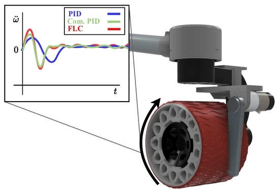
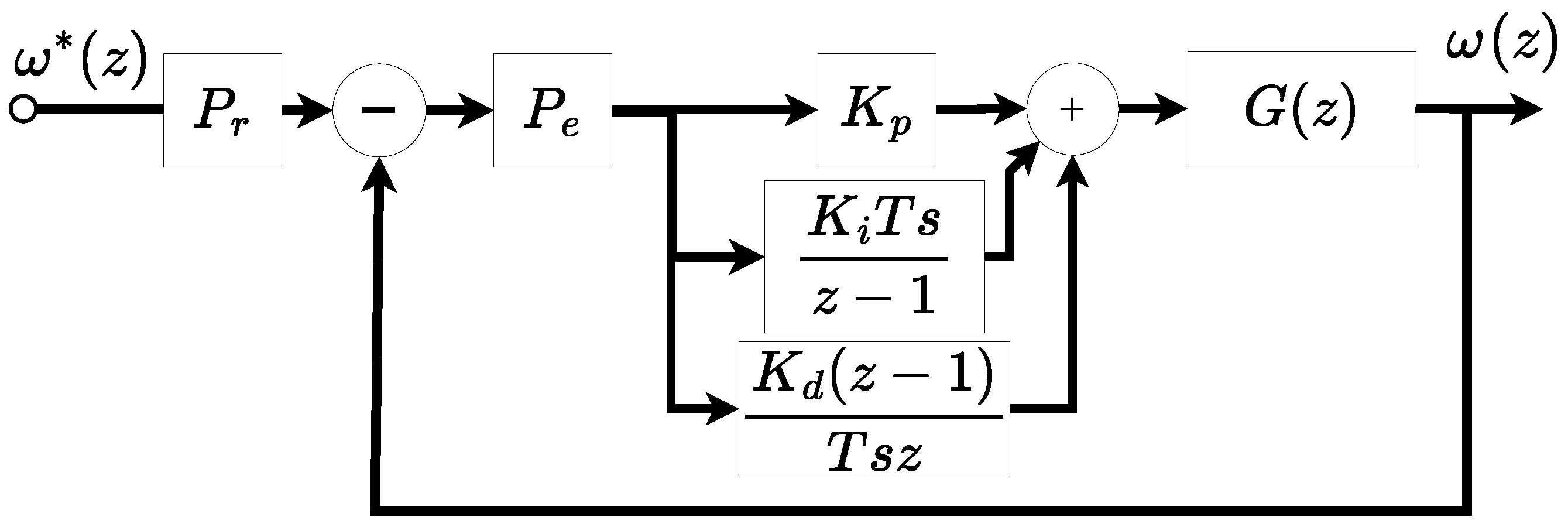
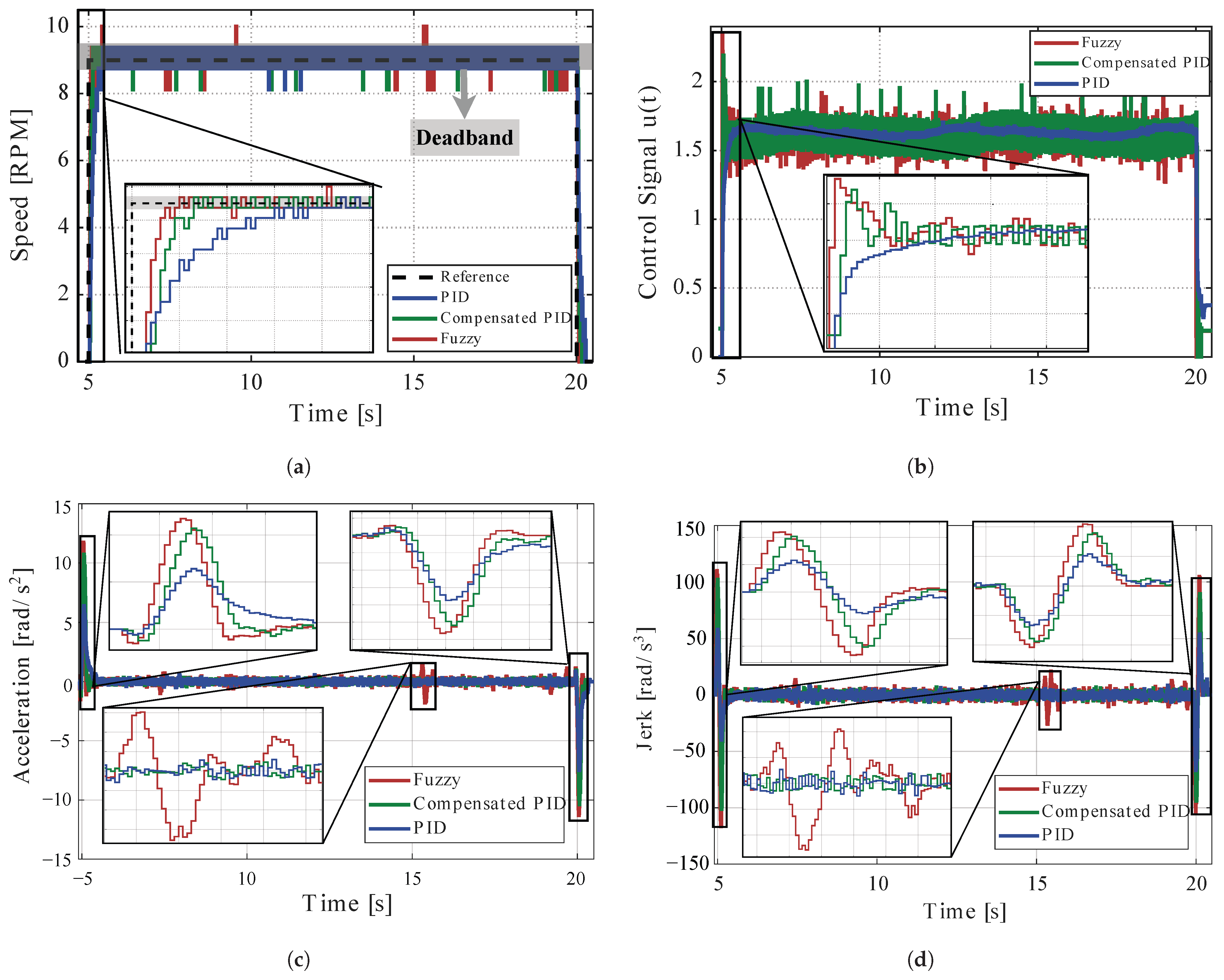
In response to this limitation, this work presents an experimental comparative analysis of different control strategies applied to a permanent magnet DC (PMDC) motor integrated in an educational rover designed for exploration of uneven terrain. Three widely studied control approaches are evaluated: a classical PID controller, an analytically compensated PID designed through discrete pole placement, and a fuzzy logic controller optimized according to the speed tracking and error requirements of the system. Consistent with the evaluation methodologies commonly reported in the state of the art, the proposed controllers are first assessed using conventional transient response metrics, including overshoot, steady-state error, and settling time, as these criteria remain standard references for determining control strategy effectiveness. Beyond these traditional indicators, however, the work incorporates an additional analysis dimension based on kinematic behavior, encompassing velocity, acceleration, and jerk profiles. The objective is not to replace classical evaluation criteria, but to complement them through a broader characterization of controller performance on a real robotic platform subject to realistic operating conditions.

2. Experimental Platform and Embedded Control System

PRAXIA is a mobile robotic platform configured as a rover with six wheels, developed by the Research Group on Interaction, Robotics and Automation (GIIRA) at Universidad Politécnica Salesiana (Cuenca, Ecuador). The platform was conceived as an educational experimental platform for applications in terrestrial environmental monitoring, precision agriculture support, industrial safety, and additive manufacturing process validation. To this end, it integrates a sensor network capable of measuring temperature, relative humidity, vapor and gas concentration, ambient light intensity, and ultraviolet radiation.

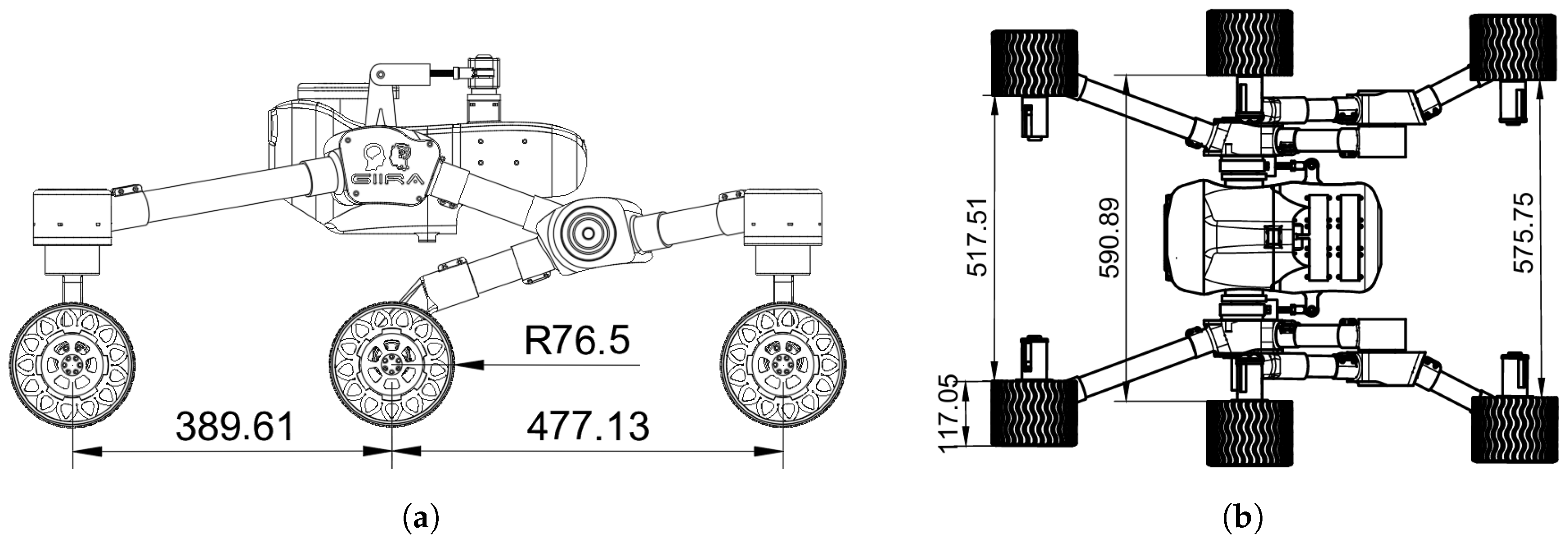
The chassis incorporates a passive rocker bogie suspension system, which distributes the platform weight evenly across the six drive units and ensures continuous wheel contact with the ground on uneven terrain. The measured dimensions of the rover are presented in Figure 1.

The software architecture is implemented on the Robot Operating System (ROS) ecosystem, structured as a set of distributed nodes communicating through publish and subscribe mechanisms. Advanced processing tasks, including teleoperation, telemetry management, and visual perception via a depth camera, are handled by an NVIDIA Jetson Nano module.

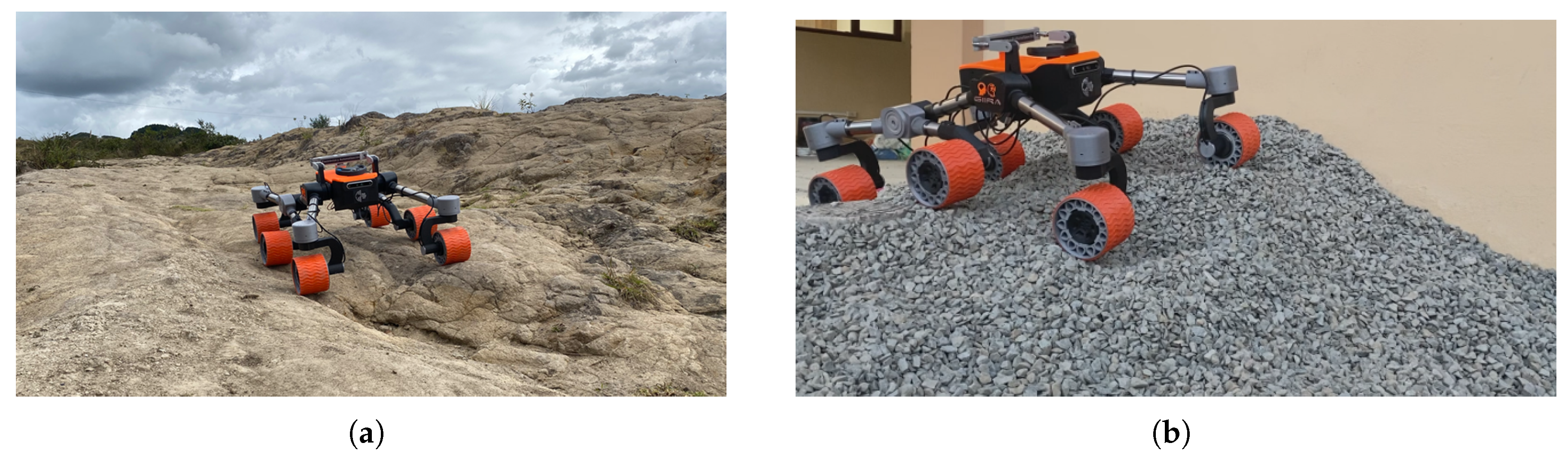
The navigational capability of the platform on unstructured terrain was assessed through experimental trials across multiple surface types, as illustrated in Figure 2. Traction limitations were identified on loosely compacted sandy terrain, attributed to the reduced substrate adhesion.

Individual wheel speed control is therefore essential for autonomous navigation, requiring controllers that achieve fast reference tracking, minimal overshoot, and convergent steady-state error.

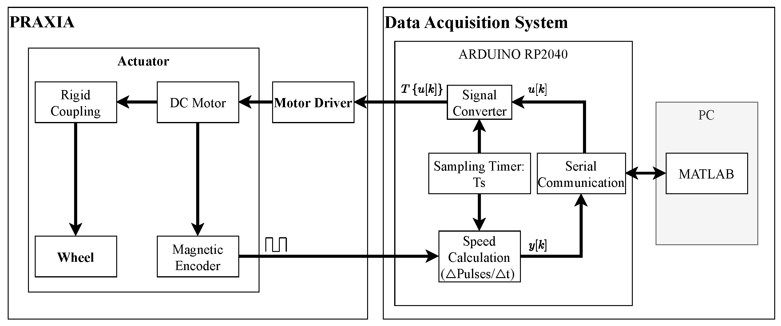
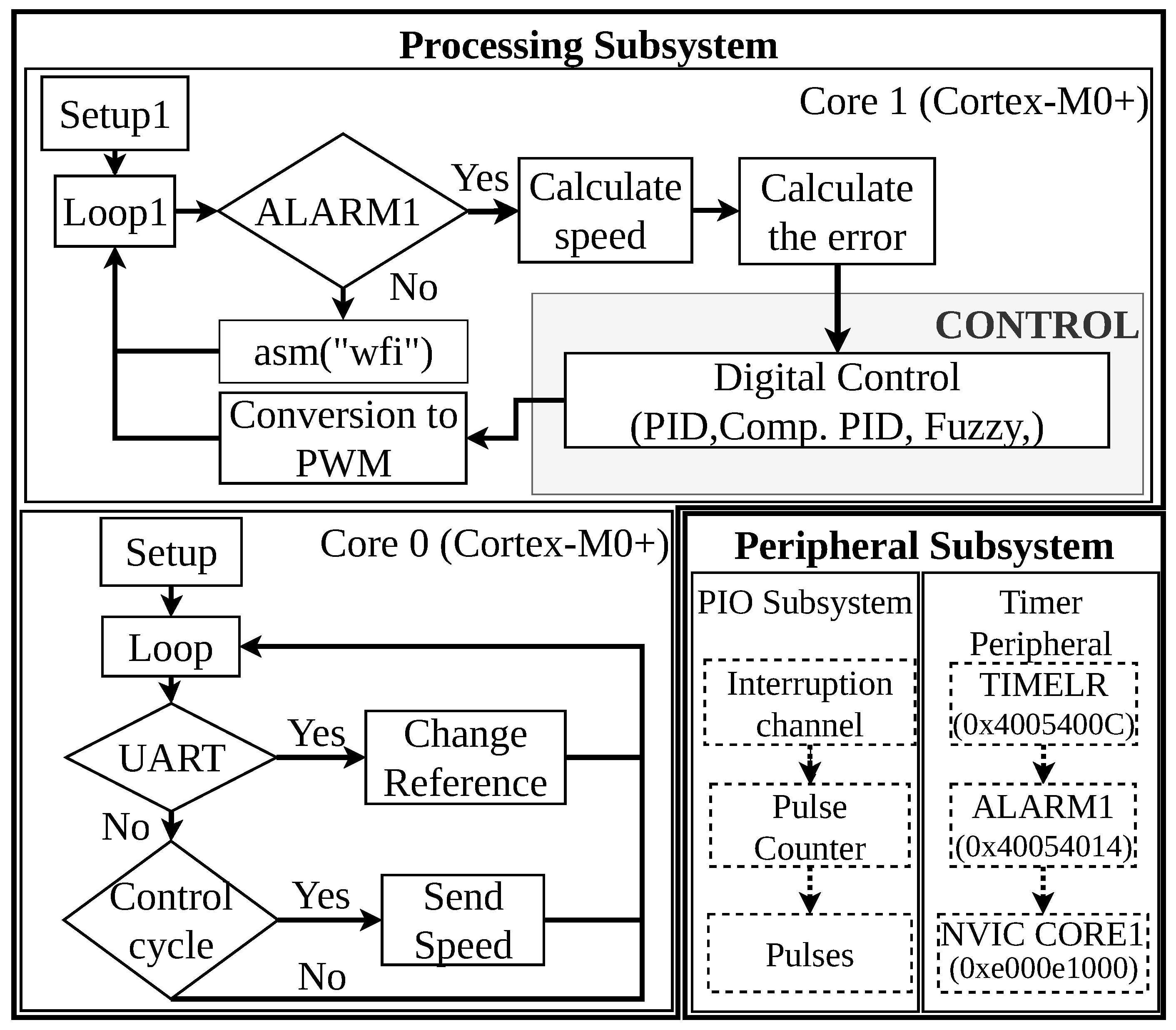
Each wheel is independently driven by an actuation unit consisting of a PMDC motor and a mechanical support structure. The observable variable of the system is the actuator angular velocity $\omega$, while the control input corresponds to the armature voltage V. Both parameters are managed entirely within an Arduino RP2040 Nano Connect microcontroller that executes the digital control loop, as illustrated in the general operation scheme in Figure 3.

This angular velocity is estimated from the encoder pulse count within the sampling period $\Delta t$. By defining $N_p$ as the number of detected pulses and $\mathcal{R}$ as the encoder resolution in pulses per revolution, the velocity calculation is computed according to Equation (1):

$$\omega ={\displaystyle \frac{N_p}{\mathcal{R}}}·{\displaystyle \frac{60}{\Delta t}};\left[\mathrm{RPM}\right]$$

(1)

For the experimental setup, the encoder operates with a resolution of $\mathcal{R}=9600$ pulses per revolution. Angular velocity was estimated using the frequency measurement method, in which encoder pulses are accumulated over the fixed sampling interval $T_s$. This approach was selected because of its simplicity, low computational cost, and direct compatibility with the fixed rate discrete control architecture adopted in this work. Although period-based techniques can improve velocity resolution, particularly at low-speeds, they generate measurements at a variable update rate that must subsequently be synchronized with the controller execution cycle and may become more sensitive to timing jitter and other measurement nonidealities at high pulse rates. Given the high pulse density provided by the encoder, the fixed window approach was considered a suitable compromise between implementation simplicity and measurement resolution [35].

It should be noted that on the PRAXIA platform, measurement jitter could be largely eliminated by precisely measuring the intervals between encoder pulses using the RP2040 hardware interrupts, which provide sub-microsecond timing resolution. However, the fixed-window approach was deliberately retained to evaluate controller behavior under the sensing constraints typical of lower-capability embedded platforms, where interrupt-based period measurement is not always feasible.

With $\mathcal{R}$ and $T_s$, the resulting quantization step is $\Delta {\omega }_c=2\pi /\left(\mathcal{R}{T}_s\right)=0.0654$ rad/s.

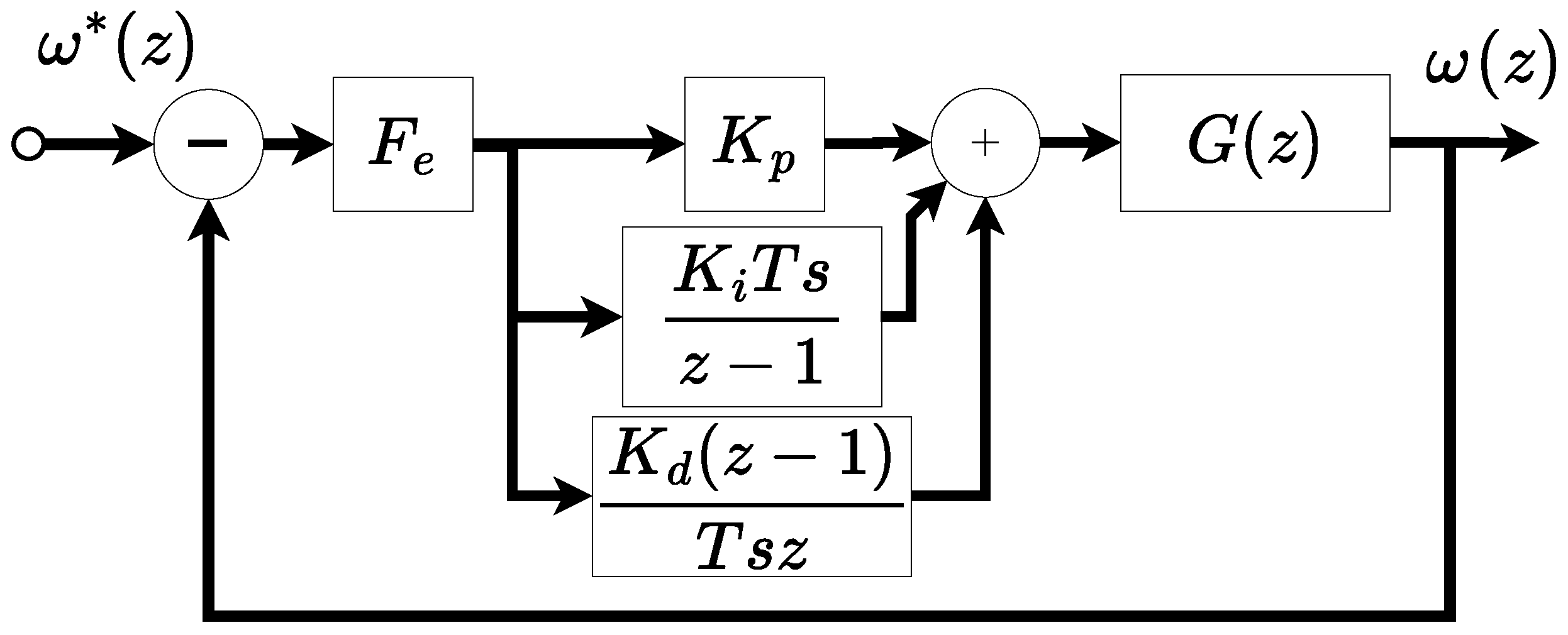
Figure 4 illustrates the implementation architecture within the microcontroller, including the execution sequence driven by a timer and the integration of the three evaluated control strategies. This structure ensures homogeneous operating conditions, thereby eliminating potential biases and enabling the intrinsic behavior of each strategy to be evaluated under identical hardware constraints.

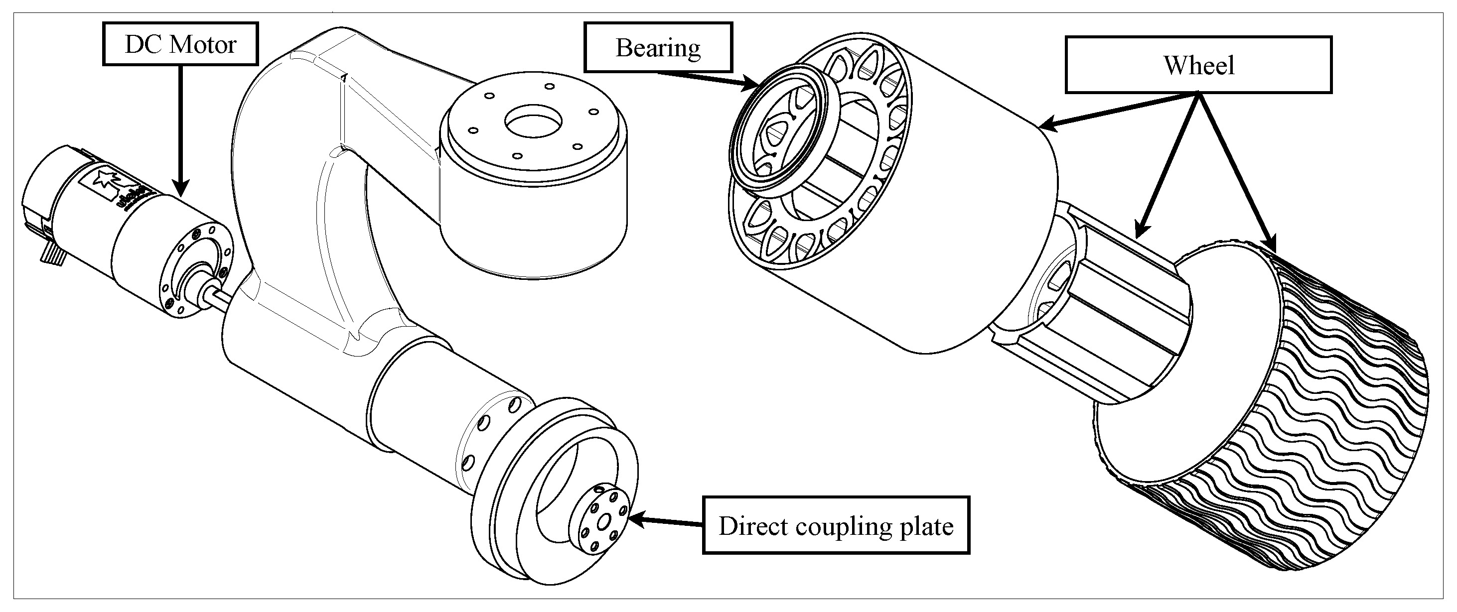
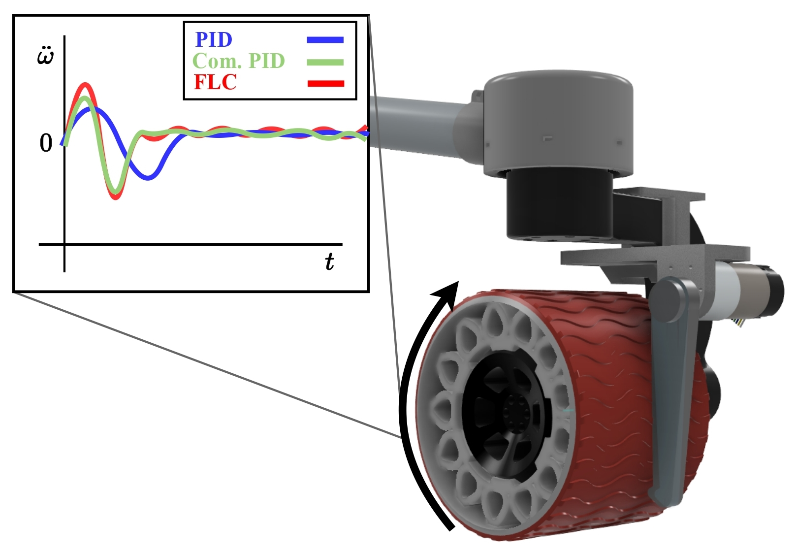
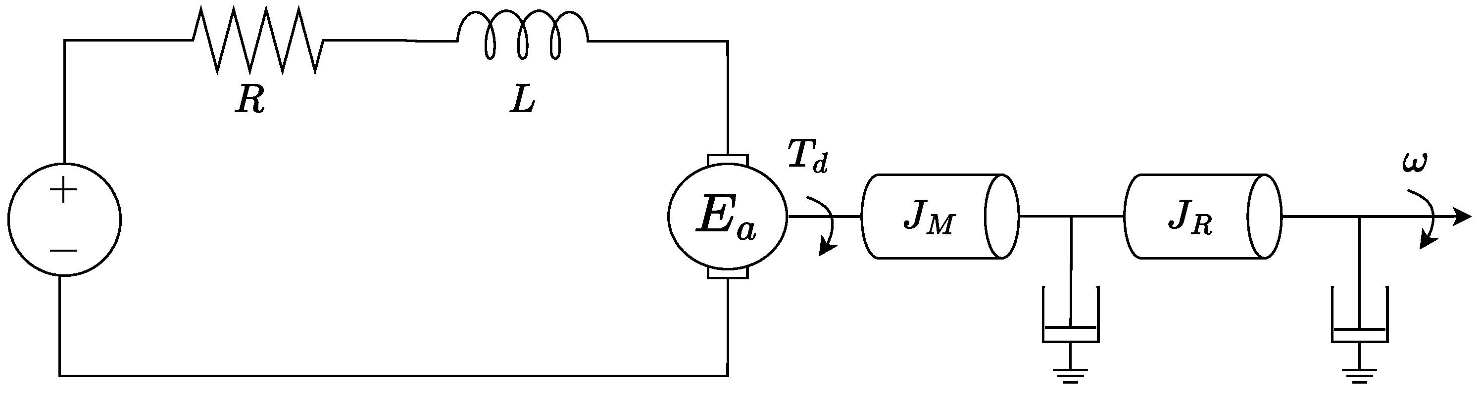
The actuation unit under study is part of the robot’s traction system. It consists of a PMDC motor and a mechanical support structure, as illustrated in Figure 5. Two mechanical interactions are critical for modeling: the direct plate coupling between the motor shaft and the wheel axle, and the bearing assembly responsible for distributing forces between them.

2.1. System Modeling and Identification

These interactions are jointly represented in the electromechanical model shown in Figure 6, where R and L denote the armature resistance and inductance, respectively; $T_d$, the electromagnetic torque; $J_M$ and $J_R$, the motor and wheel inertias; and ${\beta }_M$ and ${\beta }_R$, the viscous friction coefficients of each component.

To reduce the parametric complexity of the model, the inertial and dissipative contributions of the motor and the wheel are merged into the equivalent system parameters given by (2). This simplification is valid, assuming a rigid coupling between the motor shaft and the wheel.

$$J=J_M+J_R,\beta ={\beta }_M+{\beta }_R$$

(2)

where J represents the total moment of inertia of the system and $\beta$ the equivalent viscous friction coefficient.

From the electrical and mechanical equations of the DC motor, the second-order state-space model presented in (3) is directly obtained. The state vector is defined as $\mathbf{x}={\left[x_1{x}_2\right]}^T$ (where $x_1=\omega$ and $x_2=\dot{\omega }$) while $u=V$ represents the control input and K denotes the motor’s electromechanical constant.

$$\dot{\mathbf{x}}=\left[\begin{array}{cc}0& 1\\ -{\displaystyle \frac{R\beta +K^2}{LJ}}& -{\displaystyle \frac{L\beta +RJ}{LJ}}\end{array}\right]\mathbf{x}+\left[\begin{array}{c}0\\ {\displaystyle \frac{K}{LJ}}\end{array}\right]u$$

(3)

The dynamic behavior of the system is determined by the eigenvalues of the state matrix, obtained from the characteristic polynomial associated with (3). Experimental observations of the motor show that the system operates in an overdamped regime, under which these roots are real and negative, as expressed in (4).

$${\lambda }_{1,2}={\displaystyle \frac{-(L\beta +RJ)\mp \sqrt{{(L\beta +RJ)}^2-4LJ(R\beta +K^2)}}{2LJ}}$$

(4)

The experimental characterization reveals a marked separation of time scales between the two eigenvalues, as expressed in (5).

$$|{\lambda }_1|=a|{\lambda }_2|,a\gg 1$$

(5)

Therefore, ${\lambda }_2$ governs the $2\%$ settling time, denoted as $t_{ss}$, according to (6).

$${\lambda }_2={\displaystyle \frac{ln\left(0.02\right)}{t_{ss}}}$$

(6)

2.2. Parametric Identification

For parameter estimation, a structural approach based on physical measurements at various steady-state operating levels is adopted, in contrast to the black-box methods provided by the MATLAB R2024b system identification toolbox, which serves here as a validation reference. This approach allows K to be estimated through a least squares fit over the experimental dataset, resulting in:

$$K={\displaystyle \frac{{\sum }_{i=1}^n{\omega }_i{V}_i-R{\sum }_{i=1}^n{\omega }_i{I}_i}{{\sum }_{i=1}^n{\omega }_i^2}}$$

(7)

where I denotes the current at steady state. Once K is computed, the viscous friction coefficient is obtained as:

$$\beta =K{\displaystyle \frac{{\sum }_{i=1}^n{\omega }_i{I}_i}{{\sum }_{i=1}^n{\omega }_i^2}}$$

(8)

Finally, the equivalent moment of inertia is obtained by substituting ${\lambda }_2$ from (6) into the following expression:

$$J={\displaystyle \frac{K^2+\beta R-\beta L{\lambda }_2}{-L{\lambda }_2^2+R{\lambda }_2}}$$

(9)

This procedure obtains, in a systematic way and without additional instrumentation, the parameters that cannot be directly measured from the system. The parameterization was carried out over the six actuators of the robot, obtaining consistent results with small variations.

Table 1. Nominal parameters and statistical variability across the 6 actuators.

Parameter	$\mathit{\mu }$	$\mathit{\sigma }$ (±)	Units
R	1.95	0.0267	$\mathrm{\Omega }$
L	0.0018	0.0002	H
K	1.4010	0.0213	V·s/rad
$\beta$	0.0554	0.0025	N·m·s/rad
J	0.0543	0.0017	kg·m2

Note: The values of $\sigma$ represent the standard deviation observed across the set of 6 actuators.

summarizes the nominal values and the observed statistical dispersion.

2.3. Discretization and Transfer Function

From the mean values obtained in the parametric identification, the dominant eigenvalue of the actuators is ${\lambda }_2=-19.90$, corresponding to a time constant $\tau =50.2\mathrm{ms}$ and a $2\%$ settling time of approximately $196\mathrm{ms}$. The selected sampling frequency $f_s=100\mathrm{Hz}$ provides approximately 5 samples per time constant and 20 samples over the full transient response. The corresponding sampling period is $T_s=0.01\mathrm{s}$. Although a higher sampling rate would increase the number of samples per time constant, the fixed-window velocity estimation method constrains this choice: the quantization step $\Delta {\omega }_c=2\pi /\left(\mathcal{R}{T}_s\right)$ is inversely proportional to $T_s$, so halving the sampling period would double the measurement noise injected into the control loop, which is particularly detrimental at the low reference speeds considered in this work.

For the implementation of the digital controller, the continuous state-space model is discretized using zero order hold (ZOH) with sampling period $T_s$, yielding the discrete system:

$$\mathbf{x}[k+1]=A_d\mathbf{x}\left[k\right]+B_{d}u\left[k\right],{\omega }_c\left[k\right]=C_d\mathbf{x}\left[k\right]$$

(10)

where $C_d=\left[\begin{array}{cc}1& 0\end{array}\right]$, ${\omega }_c\left[k\right]$ represents the continuous angular velocity of the actuator, and $A_d$ and $B_d$ denote the discrete state and input matrices, respectively.

From the eigenvalues ${\lambda }_1$ and ${\lambda }_2$ of the continuous state matrix, the discrete matrices $A_d$ and $B_d$ are, in principle, obtained exactly through the matrix exponential. However, since $|{\lambda }_1| \gg |{\lambda }_2|$, the discrete contribution of the fast pole satisfies $e^{{\lambda }_1{T}_s}\approx 0$ under the selected sampling period, This condition allows the simplification of the matrix exponential in discretization Equations (11) and (12) without compromising dynamic fidelity, as demonstrated through simulation.

$$A_d=\left[\begin{array}{cc}{\displaystyle \frac{{\lambda }_1{e}^{{\lambda }_2{T}_s}}{{\lambda }_1-{\lambda }_2}}& -{\displaystyle \frac{e^{{\lambda }_2{T}_s}}{{\lambda }_1-{\lambda }_2}}\\ {\displaystyle \frac{{\lambda }_1{\lambda }_2{e}^{{\lambda }_2{T}_s}}{{\lambda }_1-{\lambda }_2}}& -{\displaystyle \frac{{\lambda }_2{e}^{{\lambda }_2{T}_s}}{{\lambda }_1-{\lambda }_2}}\end{array}\right],$$

(11)

$$B_d=\left[\begin{array}{c}-{\displaystyle \frac{{\lambda }_1(e^{{\lambda }_2{T}_s}-1)+{\lambda }_2}{{\lambda }_1{\lambda }_2({\lambda }_1-{\lambda }_2)}}\\ -{\displaystyle \frac{e^{{\lambda }_2{T}_s}}{{\lambda }_1-{\lambda }_2}}\end{array}\right].$$

(12)

Furthermore, for controller design via pole placement, it is advantageous to express the model in transfer function form within the z domain, defined as:

$$G\left(z\right)=C_d{(zI-A_d)}^{-1}{B}_d={\displaystyle \frac{n_{1}z+n_0}{z^2-tr\left(A_d\right)z+det\left(A_d\right)}}.$$

(13)

Since $det\left(A_d\right)=0$, the denominator factorizes as:

$$z^2-tr\left(A_d\right)z=z(z-p),$$

(14)

which reveals the presence of a pole at the origin. The transfer function then takes the structural form (15).

$$G\left(z\right)=k_m{\displaystyle \frac{z+a}{z(z-p)}},$$

(15)

2.4. Model Validation

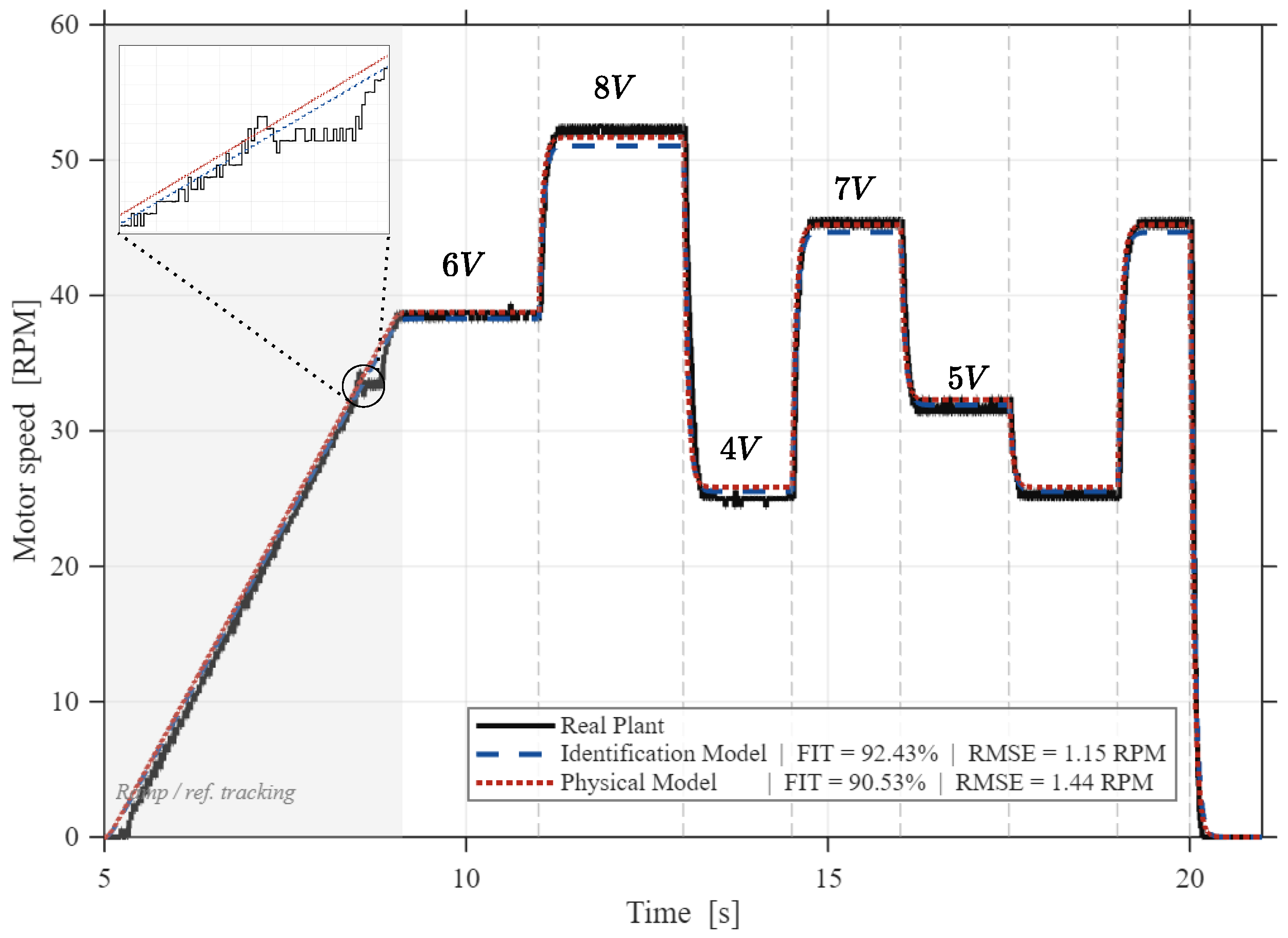
Figure 7 compares the proposed physical model against the numerical identification results from MATLAB R2024b. While the numerical approach yields a lower transient error, the physical model more accurately captures the steady-state behavior, justifying its use in controller design.

2.5. Encoder Quantization Model

From the estimated continuous velocity ${\omega }_c\left[k\right]$, the equivalent number of encoder increments is computed as:

$$n\left[k\right]={\displaystyle \frac{{\omega }_c\left[k\right]}{\Delta {\omega }_c}}$$

(16)

Since $n\left[k\right]$ is generally non-integer, the quantized increment count $n_q\left[k\right]$ is obtained by rounding to the nearest integer:

$$n_q\left[k\right]=\mathrm{round}\left(n\left[k\right]\right)$$

(17)

where, in the boundary case $n\left[k\right]=\lfloor n\left[k\right]\rfloor +0.5$, a randomized rounding rule is applied with equal probability for both outcomes, so as to avoid systematic bias in the quantization error. The quantized velocity delivered to the controller at each sampling instant is then recovered as:

$$\omega \left[k\right]=n_q\left[k\right]·\Delta {\omega }_c$$

(18)

3. Design and Tuning of Model-Based PID Controllers

Two design strategies are derived from the discrete transfer function in (15). The first is an analytical approach based on discrete pole placement, which explicitly incorporates the plant dynamics and the desired closed-loop specifications. The second is a model-based tuning procedure implemented using the MATLAB R2024b PID Tuner, representing a conventional industrial design workflow. Both controllers are evaluated using the same transient-response and steady-state performance metrics to ensure a consistent and objective comparison.

3.1. Analytical Design by Pole Placement with Precompensation

An analytical design method based on pole placement in discrete time is employed to achieve a closed-loop response that directly meets the specified dynamic requirements. Unlike empirical tuning, this approach derives the controller parameters from the plant model and the closed-loop poles, ensuring a systematic and reproducible design.

Based on the plant model and within the pole placement design framework, two precompensators are introduced: an error precompensator $P_e\left(z\right)$, used to cancel the plant zero $z=-a$, and a reference precompensator $P_r\left(z\right)$, used to achieve the desired second-order response. These precompensators are defined as:

$$\begin{array}{c}{P}_e\left(z\right)={\displaystyle \frac{z}{z+a}},P_r\left(z\right)={\displaystyle \frac{q_0+q_1+q_2}{q_0{z}^2+q_{1}z+q_2}}\end{array}$$

(19)

A noteworthy consequence of this analytical construction is the inherent attenuation of high-frequency components in both the reference and error channels. This property emerges naturally from the imposed closed-loop dynamics and should be regarded as a byproduct of the pole placement formulation rather than as an explicit filtering mechanism. Together with the PID gains, these precompensators yield the complete controller parameterization:

$$\mathbf{q}=\left[\begin{array}{c}{q}_0\\ q_1\\ q_2\end{array}\right],{\mathbf{k}}_{\mathrm{PID}}=\left[\begin{array}{c}{k}_p\\ k_i\\ k_d\end{array}\right]$$

(20)

The design procedure imposes a desired dynamics of second-order in closed-loop characterized by the damping ratio ${\zeta }_d$ and natural frequency ${\omega }_d$. These specifications determine the auxiliary parameters:

$$\begin{array}{c}A=e^{-T_s{\zeta }_d{\omega }_d},B=cos\left(T_s{\omega }_d\sqrt{1-{\zeta }_d^2}\right)\end{array}$$

(21)

Matching the desired characteristic polynomial with the denominator of the closed-loop yields the precompensator coefficients analytically:

$$\begin{array}{c}\mathbf{q}={\displaystyle \frac{1}{k_m}}\left[\begin{array}{c}ϵ-2AB+1-p\\ A^2-2ABϵ+p\\ A^2ϵ\end{array}\right]\end{array}$$

(22)

where $ϵ$ corresponds to an auxiliary pole that is not dominant, introduced to make both the numerator and denominator degrees compatible, whose contribution to the dynamics of the closed-loop is negligible by design.

The discrete PID gains are then recovered algebraically from $\mathbf{q}$ through:

$$\begin{array}{c}{\mathbf{k}}_{\mathrm{PID}}=\left[\begin{array}{ccc}1& 0& -1\\ T_s^{-1}& T_s^{-1}& T_s^{-1}\\ 0& 0& T_s\end{array}\right]\mathbf{q}\end{array}$$

(23)

This mapping establishes a direct and invertible relationship between the poles of the closed-loop and the PID gains, with no free tuning parameters beyond the performance specifications $({\zeta }_d,{\omega }_d)$. For this application, specifications prioritizing fast response with minimal overshoot were selected to avoid traction losses during speed transients: a maximum overshoot of $0.1\%$ and a peak time $t_p=150\mathrm{ms}$, conditioned by the actuator’s physical limitations to ensure realizable gains. The resulting parameters are listed in

Table 2. Parameters and gains of the compensated discrete PID controller.

Parameter	Symbol	Value
Difference Equation Coefficients
Coefficient $q_0$	$q_0$	3.1687
Coefficient $q_1$	$q_1$	−2.3972
Coefficient $q_2$	$q_2$	0.0392
PID Controller Gains
Proportional Gain	$k_p$	3.1296
Integral Gain	$k_i$	81.0711
Derivative Gain	$k_d$	0.00039
Filter Parameter
Compensation zero	a	−0.052

.

The final structure of the control system is presented in Figure 8, where the compensation filters are integrated with the discrete PID controller.

3.2. Standardized Signal Conditioning for Comparative Evaluation

To ensure a rigorous methodological comparison between the analytically designed PID controller and alternative control strategies, the inherent signal conditioning introduced by the error precompensator $P_e\left(z\right)$ must be addressed. As established in Equation (19), $P_e\left(z\right)$ incorporates a pole at $z=0.052$ and a zero at the origin. Frequency response analysis of this discrete block reveals a unitary gain cross-over point at exactly $24.58\mathrm{Hz}$ (for a sampling period $T_s=10\mathrm{ms}$). Beyond this frequency, the precompensator inherently provides progressive attenuation of high-frequency components, effectively acting as a noise suppression mechanism for the PID control loop. To prevent this inherent filtering from providing an uncompensated signal-to-noise advantage to the PID structure during comparative evaluations, a standardized first-order low-pass filter is implemented in the error channel of the alternative controllers. The cutoff frequency of this filter is matched exactly to the $24.58\mathrm{Hz}$ cross-over point of $P_e\left(z\right)$. This standardizes the high-frequency noise rejection across all evaluated strategies without transferring the low-frequency static gain bias inherent to the analytical precompensator. The normalized discrete transfer function of the comparative filter is defined as:

$$F_e\left(z\right)={\displaystyle \frac{(1-\rho )z}{z-\rho }}$$

(24)

where the discrete pole $\rho$ is determined through the exact z-plane mapping $\rho =e^{-2\pi f_c{T}_s}$. To match the target cutoff frequency of $f_c=24.58\mathrm{Hz}$ at the predefined sampling period, the parameter is set to $\rho =0.2134$. This standardized signal conditioning guarantees that all controllers operate under equivalent dynamic measurement conditions. Any observed variance in transient performance or steady-state accuracy during the physical implementation can therefore be attributed strictly to the mathematical formulation of the respective control laws, isolating the hardware variables from the comparative analysis.

3.3. Classical Method

As a baseline, a PID controller is tuned using MATLAB R2024b PID Tuner, leveraging the identified actuator model together with the error filter $F_e\left(z\right)$ described in Section 3.2. The filter is incorporated during the tuning stage so that the resulting controller parameters account for the same measurement-noise conditioning applied during experimental validation. While empirical methods like Ziegler–Nichols are viable, PID Tuner facilitates a model-based approach aligned with Internal Model Control (IMC) principles [36]. This allows us to systematically adjust the balance between response speed and robustness via a single tuning parameter, ensuring a fair and quantifiable comparison against the other evaluated strategies.

The discrete model of the classical PID controller is given by

$$u\left[k\right]=K_{p}e\left[k\right]+K_i{T}_s{\displaystyle \sum _{j=0}^k}e\left[j\right]+{\displaystyle \frac{K_d}{T_s}}\left(e\left[k\right]-e[k-1]\right)$$

(25)

where $u\left[k\right]$ is the control signal and $e\left[k\right]$ is the tracking error at sample k. The tuning objective is to obtain a fast response with minimal overshoot and adequate disturbance rejection capability while maintaining stable actuator operation.

The selected parameters were obtained through a systematic sweep of the two tuning controls available in the MATLAB R2024b PID Tuner: the response time ${\tau }_c$, which determines the bandwidth of the closed-loop, and the transient behavior parameter $\alpha \in [0,1]$, which balances controller aggressiveness and robustness.

Table 3. Representative operating points from the PID tuning sweep, organized by transient behavior parameter.

	Sweep Points
${\tau }_c$ (s)	2.405	1.384	0.264	0.200	0.200	0.200
$\alpha$	0.459	0.693	0.693	0.693	0.792	0.900
$K_p$	0.0126	0.0220	0.1999	0.4472	0.7232	0.9970
$K_i$	1.2615	2.1956	12.1962	16.6385	16.2739	15.0914
$K_d$	$3.15\times {10}^{-5}$	$5.49\times {10}^{-5}$	0.0008	0.0030	0.0080	0.0109
Rise time (s)	2.51	1.39	0.19	0.15	0.18	0.22
Settling time (s)	4.53	2.53	0.29	0.36	0.27	0.40
Overshoot (%)	0.00	0.00	1.58	2.65	0.18	0.00
Phase margin (°)	87.4	85.4	69.3	69.3	79.2	90.0

Bold values indicate the selected controller configuration.

presents representative operating points from this tuning process. In accordance with the design objectives, particular emphasis was placed on achieving a fast response with negligible overshoot while ensuring satisfactory performance during experimental validation.

The selected configuration was chosen for its acceptable rise time and zero overshoot with a phase margin of 90°, ensuring a stable response. Finally, the control architecture is represented by the block diagram shown in Figure 9, corresponding to the PID implementation in discrete time adopted in this work.

4. Design and Parametric Optimization of a Fuzzy Controller

The fuzzy controller is developed as an alternative to the PID controller, with the objective of evaluating its performance under the same operating conditions, particularly in the presence of disturbances, nonlinearities, and variations in the system dynamics. Unlike the conventional approach, fuzzy control is based on heuristic knowledge, represented through linguistic rules that describe the desired system behavior, whose gains are parametrically optimized to minimize the tracking error based on the obtained model.

The implemented architecture is shown in Figure 10. This structure integrates the computation of the speed error and its derivative with the fuzzy inference system, generating a control variation signal $\Delta u$ applied to the actuator. The inclusion of the error derivative as an input variable allows the controller to anticipate the dynamic trend of the system, acting in a preventive manner in the presence of imminent changes in speed before the error propagates. In turn, the incremental variation action at the output implicitly introduces an integrating effect in the control signal applied to the actuator, which contributes to reducing the error at steady state.

4.1. Input Variables, Universe of Discourse, and Membership Functions

The design of the universe of discourse is based on the physical limitations of the implemented discrete system. As established in Section 2, the minimum resolution of the speed measurement from the encoder on the RP2040 microcontroller is $\Delta \omega$. This value defines the boundary of the system deadband: speed errors below this threshold must be considered as an acceptable region, since they lie within the measurement quantization noise. Consequently, the minimum significant error limit is established, and analogously, the error derivative exhibits the same effective resolution limit, $|{\dot{e}}_{min}|=(0.0654/Ts){\mathrm{rad}/\mathrm{s}}^2$, since it is computed as the difference between consecutive measurements subject to the same quantization.

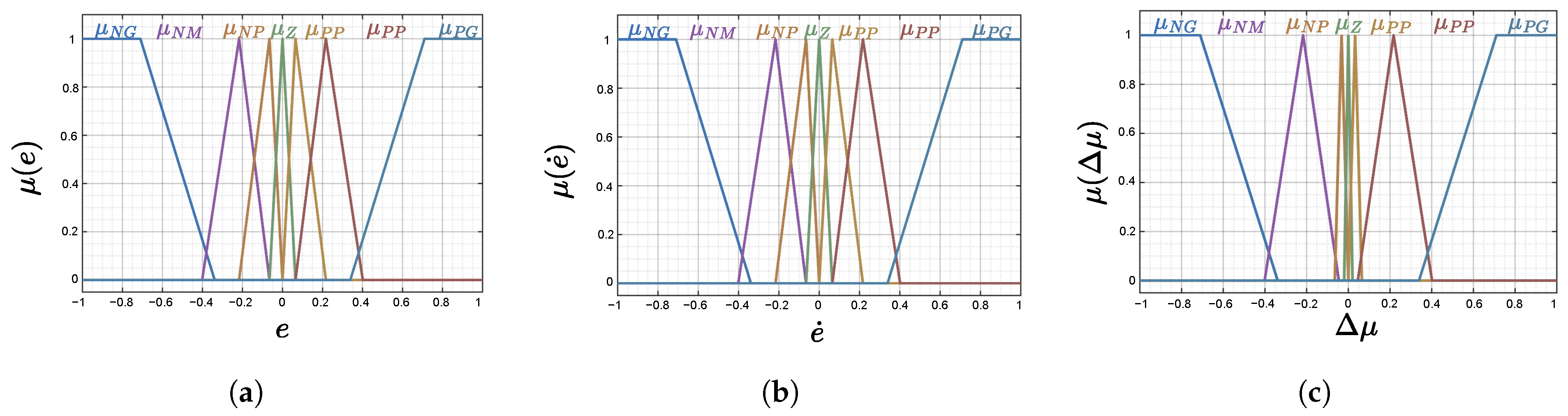
The membership functions for the input and output variables are illustrated in Figure 11. The inputs e and $\Delta e$ are classified into seven categories, NG, NM, NP, Z, PP, PM, and PG; analogously, the output $\Delta V$ is classified into VH, MH, H, M, L, ML, and VL, in order to satisfy the system requirements: fast response and minimal overshoot, within the voltage saturation limits of the actuator.

4.2. Inference Rules

The inference rule base, shown in

Table 4. Fuzzy inference rule base for the proposed controller.

$\mathit{e}\setminus \mathbf{\Delta }\mathit{e}$	NG	NM	NP	Z	PP	PM	PG
NG	VL	VL	VL	VL	VL	ML	ML
NM	VL	ML	ML	L	L	L	H
NP	ML	L	L	L	L	H	H
Z	L	L	L	M	H	H	H
PP	L	L	M	H	H	H	MH
PM	L	M	H	H	MH	MH	VH
PG	H	MH	VH	VH	VH	VH	VH

, was defined according to the specific requirements of the system. An inference mechanism of the Mamdani type was employed, with defuzzification using the centroid method.

The design procedure, which includes the selection of input variables, membership functions, their corresponding ranges, and the rule base, was based on configurations reported in previous studies [14,15,27,28,29]. These configurations were adapted to the specific conditions of the system.

Additionally, the type of membership functions was selected considering the feasibility of implementation on a microcontroller operating at a control frequency of 100 Hz.

4.3. Parameterization and Optimization of the Fuzzy Controller

Unlike the PID controller, the fuzzy controller does not have an analytical method that guarantees the effectiveness of the rule base or the membership functions. Therefore, the normalization gains ($G_e$, $G_{\dot{e}}$, $G_s$) were tuned via differential evolution, minimizing a composite cost function that jointly penalizes the three performance criteria identified in the literature review: tracking error, response speed, and overshoot:

$$\mathcal{J}=T_s{\displaystyle \sum _{k=0}^N}\left|e\left[k\right]\right|+0.5t_r+8max\left(0,\%\overline{OS}-1\%\right)$$

(26)

where $t_r$ is the rise time ($10$–$90\%$) and $\%OS$ is the percentage overshoot. The search ranges were determined from values reported in the literature. The optimizer was configured with a population size of $N_p=15$, a convergence tolerance of $\epsilon ={10}^{-7}$, and a fixed seed to ensure reproducibility of the results. The obtained gains are presented in

Table 5. Controller gains obtained through the optimization process.

${\mathit{G}}_{\mathit{e}}$	${\mathit{G}}_{\mathbf{\Delta }\mathit{e}}$	${\mathit{G}}_{\mathit{s}}$
5.0298	36.6970	203.8953

.

The weighting coefficients were selected so that each term contributes comparably to $\mathcal{J}$ at the expected operating point, preventing any single criterion from dominating the search. This formulation mirrors the design philosophy applied to the PID strategies, ensuring that all three controllers are optimized under equivalent objectives.

5. Simulation Framework and Sensitivity Analysis

The simulated response to the step input is presented in Figure 12. The results indicate that the fuzzy controller reaches the reference faster during the transient, followed by the compensated PID. The classical PID exhibits the slowest convergence, with an exponential decay characteristic of its conservative tuning. Regarding the control effort, the classical PID produces the action with the least reactivity and lowest amplitude, with residual oscillations resulting from quantization effects introduced by the speed estimation method using a fixed window.

5.1. Jerk Metric Construction

To characterize the mechanical smoothness of each controller in steady-state conditions, the root mean square (RMS) of the jerk was computed from the angular velocity signal. The angular velocity was processed using a Savitzky–Golay (SG) differentiating filter to estimate its second time derivative. The estimated jerk J was obtained as

$$J\left[k\right]={\displaystyle \frac{1}{T_s^2}}{\displaystyle \sum _{j=-m}^m}{c}_j^{\left(2\right)}\omega [k+j],m={\displaystyle \frac{W-1}{2}},$$

(27)

where W denotes the sliding window length, and $c_j^{\left(2\right)}$ are the coefficients derived from a local polynomial fit of degree $p=3$. This degree represents the minimum order necessary to ensure a consistent second derivative estimate while effectively attenuating measurement noise. Finally, to quantify performance across different operating conditions, the instantaneous jerk estimates are condensed into a single scalar indicator by calculating the root mean square (RMS) value over N samples:

$$\mathrm{RMS}\text{-}\mathrm{J}=\sqrt{{\displaystyle \frac{1}{N}}\sum _{k=1}^N{J}^2\left[k\right]}\left[\mathrm{rad}/{\mathrm{s}}^3\right]$$

(28)

The selection of the SG filter parameters is discussed in Section 6.3. The same filtering procedure was used for both simulation and experimental data to ensure a consistent computation of the metrics related to the jerk.

The use of jerk-based metrics is motivated by previous studies showing that excessive jerk contributes to vibration excitation, actuator wear, and fatigue-related mechanical degradation. For example, Pawlus et al. demonstrated that jerk energy is directly associated with cumulative drivetrain damage and vibration severity, while van der Kruk highlighted the role of jerk in the excitation of structural resonances and actuator wear [37,38]. In the present work, the RMS value of jerk is adopted instead of the Integral of Squared Jerk (JE) commonly used in the literature.

$$\mathrm{RMS}\text{-}\mathrm{J}=\sqrt{{\displaystyle \frac{JE}{N·T_s}}}$$

(29)

The RMS formulation was selected because it provides a normalized scalar measure that is independent of signal length, facilitating consistent comparisons across operating conditions and experimental trials.

5.2. Parametric Sensitivity Analysis

In order to evaluate the statistical robustness of the comparative results against the manufacturing variability observed among the six rover actuators, a parametric sensitivity analysis was performed using Monte Carlo simulation. For each sample $i\in \{1,\dots ,N_{\mathrm{MC}}\}$, with $N_{\mathrm{MC}}=500$, a set of perturbed parameters was generated using independent uniform distributions:

$${\theta }_i={\theta }_0+{\delta }_{\theta }·{\epsilon }_i,{\epsilon }_i\sim \mathcal{U}(-1,1),$$

(30)

where $\theta \in \{R,L,K,\beta ,J\}$, ${\theta }_0$ denotes the nominal value from Table 1 and ${\delta }_{\theta }$ the corresponding experimentally measured variation bound. For each set ${\theta }_i$, the matrices $A_d^{\left(i\right)}$ and $B_d^{\left(i\right)}$ were reconstructed using expressions (11) and (12), and the full simulation described in (10) was executed with the encoder quantization logic according to (18).

The kinematic metrics were evaluated over the window at steady state $t=1$ s, which is sufficient for simulation analysis since the discrete model is deterministic, unlike the experimental environment. Metrics related to the jerk were computed using the procedure defined in Equation (27). For each metric $\varphi \in \{\mathrm{IAE},{\mathrm{RMS}}_j,\mathrm{JE}\}$ and each controller c, the sample mean ${\overline{\varphi }}_c$ and standard deviation $s_c$ were estimated according to

$${\overline{\varphi }}_c={\displaystyle \frac{1}{N_{\mathrm{MC}}}}{\displaystyle \sum _{i=1}^{N_{\mathrm{MC}}}}{\varphi }_c^{\left(i\right)},s_c=\sqrt{{\displaystyle \frac{1}{N_{\mathrm{MC}}-1}}\sum _{i=1}^{N_{\mathrm{MC}}}{\left({\varphi }_c^{\left(i\right)}-{\overline{\varphi }}_c\right)}^2},$$

(31)

The results are summarized in

Table 6. Monte Carlo sensitivity analysis ($N_{\mathrm{MC}}=500$ samples). Jerk metrics computed via SG filtering (order 3, window 21) on the steady-state window ($T=1$ s). JE computed as $\mathrm{JE}={\mathrm{RMS}}^2·T$.

Controller	IAE [rad]	RMS-J [rad/s3]	JE [rad2/s5]
Classic PID	$0.031\pm 0.000$	$12.03\pm 0.24$	$144.82\pm 5.71$
Comp. PID	$0.031\pm 0.000$	$11.88\pm 0.56$	$141.36\pm 12.79$
Fuzzy Mamdani	$0.028\pm 0.000$	$13.05\pm 0.44$	$170.58\pm 12.48$
CV (%): IAE: $0.00$/$0.07$/$0.78$;   RMSj: $1.97$/$4.72$/$3.36$;   JE: $3.94$/$9.05$/$7.32$
(Classic PID/Comp. PID/FLC).
IAE ranking: stable in $99.6\%$ of samples.   RMSj/JE ranking: stable in $65.8\%$ (PIDs statistically indistinguishable).

. As expected in a deterministic simulation subject to small parametric perturbations, the metric values across controllers remain consistent and primarily reflect the limited actuator variability considered in the analysis. The purpose of this analysis is to verify the robustness of the ordinal ranking under the parametric variability observed across the six rover actuators. The coefficients of variation remained below $0.8\%$ for the IAE across all controllers, indicating that the tracking performance is largely insensitive to the parameter variations. For the jerk-related metrics, the coefficients of variation remained below $4.8\%$ for RMS_j and below $9.1\%$ for JE, reflecting a higher but still moderate sensitivity to actuator uncertainty. The IAE ranking was stable in $99.6\%$ of the samples, confirming that the Fuzzy Mamdani controller consistently achieved the lowest tracking error. The RMS_j/JE ranking was stable in $65.8\%$ of the samples, indicating that the ordering between the two PID variants occasionally changes due to their small absolute differences rather than a structural modification of the controller behavior. Overall, these results confirm that the comparative conclusions drawn from the nominal simulation are robust to actuator variability.

6. Experimental Results and Controller Comparison

6.1. Experimental Design

The three control strategies were implemented on an RP2040 microcontroller. Experimental validation was performed using two actuators whose parameters closely match the nominal values in Table 1, as identified by our parametric sensitivity analysis. Tests were divided into two scenarios: unperturbed operation (no external load) and operation under induced mechanical disturbances.

In the unperturbed scenario, we evaluated six reference speeds ranging from 3 to 60 RPM, with emphasis on the low-speed range, where encoder quantization and measurement resolution effects are most prominent. For the disturbed scenario, we restricted the range to 3–20 RPM. This limitation was twofold: first, to mitigate mechanical wear and thermal stress caused by prolonged loading; and second, to account for the disturbance generator’s physical constraints, as its influence on actuator dynamics diminishes at higher speeds.

To ensure statistical validity, we conducted 20 repetitions per speed and controller for the scenario without perturbation (360 total experiments) and 10 for the scenario with disturbance (120 total). Finally, we assessed the performance at steady state using the RMS-J metric (Equation (28)). For each case, we calculated the sample mean and standard deviation of the RMS-J values across repetitions to quantify both the average kinematic smoothness and the variability from trial to trial.

6.2. Disturbance Signal

Controlled disturbances were introduced using a second motor with characteristics identical to those of the actuator under study. This motor was mechanically coupled to the shaft and operated in active braking mode, thereby generating a tangential force on the wheel and, consequently, a variable disturbance torque. The disturbance torque acting on the system can therefore be expressed as

$$T_{\mathrm{dist}}=r·F_{\mathrm{dist}},$$

(32)

where r denotes the wheel radius, equal to 16 cm. This term can be included in the motor mechanical equation as

$$J\dot{\omega }=T_d-\beta \omega -T_{\mathrm{dist}},$$

(33)

where $T_{\mathrm{dist}}$ represents the external disturbance torque applied to emulate variable operating conditions on the wheel. The disturbance magnitude was varied by modulating the voltage applied to the load motor, sweeping from $0\%$ to $100\%$ of the nominal voltage.

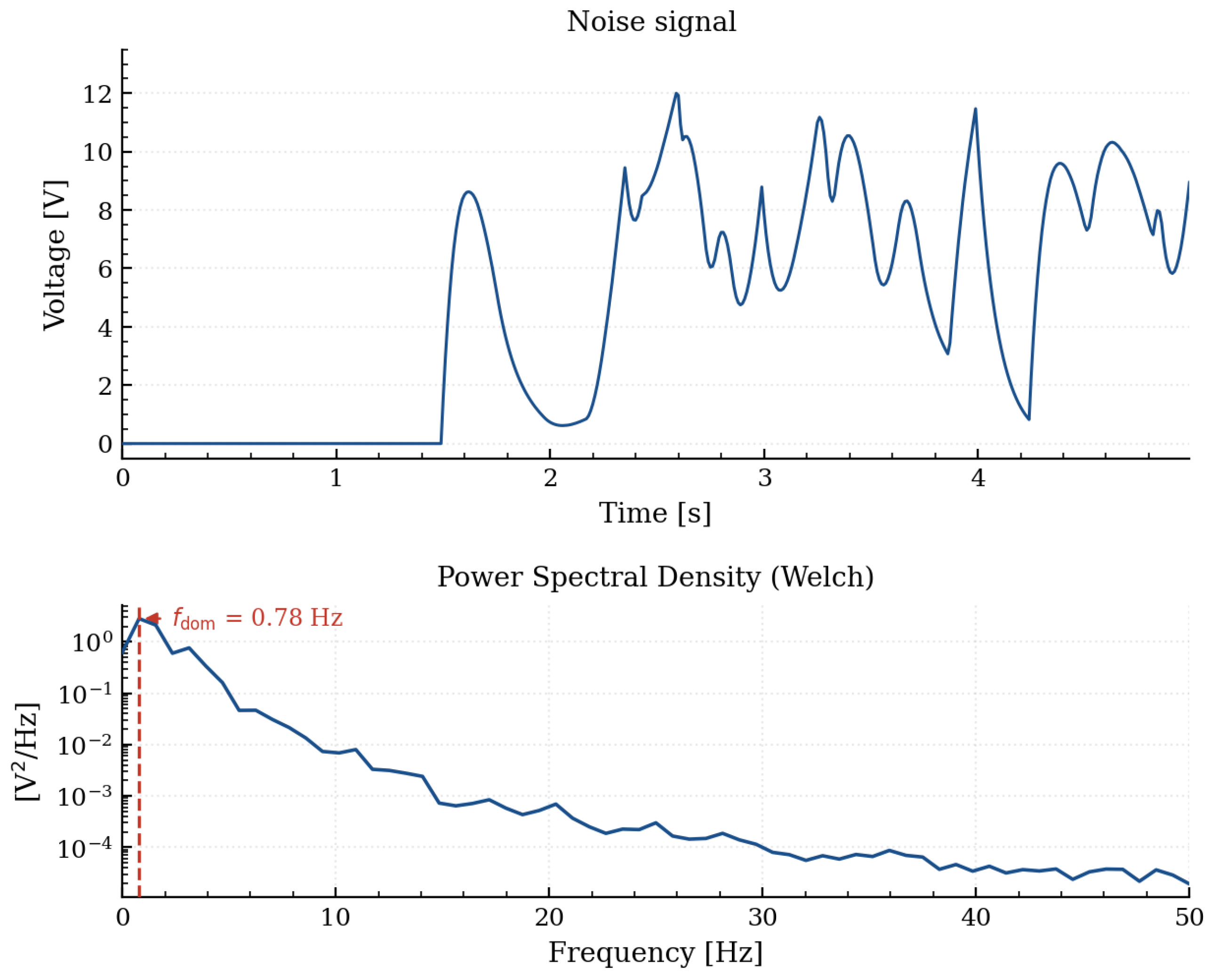
The second evaluation scenario introduces controlled disturbances with the objective of characterizing the performance of each strategy under nonlinearities and variable load conditions, emulating representative operating scenarios in real environments. The disturbance magnitude was adjusted by varying the voltage applied to the load motor between $0\%$ and $100\%$ of the nominal value, yielding the signal shown in Figure 13.

The signal exhibits a dominant frequency of $0.78$ Hz and a 95% power bandwidth of $3.91$ Hz, which concentrates practically all of the disturbance energy below 5 Hz. This slow spectral content lies well within the sampling bandwidth and the disturbance rejection capability of the evaluated controllers, ensuring that the disturbance is fully resolved without exciting high-frequency dynamics that are unmodeled. In addition, its amplitude distribution can be adjusted to avoid excessive loading of the actuator.

6.3. Unloaded Operation Results

The quantification of the jerk depends directly on the length of the window used by the Savitzky–Golay filter. Shorter windows preserve a larger portion of the content at high-frequency, whereas wider windows introduce a progressively stronger smoothing effect that attenuates rapid signal variations. As a result, the selection of this parameter can significantly influence the absolute magnitude of the estimated jerk and must therefore be carefully analyzed before comparing different controllers.

To obtain a consistent comparison, the analysis was restricted to the regime of steady-state. This decision is motivated by the fact that the evaluated controllers exhibit different convergence rates during the transient response, a characteristic that is inherently related to their design objectives and does not necessarily represent undesirable behavior. Since the tests employ step references, an analysis focused on the transient region would be dominated primarily by the response speed of each control strategy. In contrast, the steady-state regime allows the residual fluctuations of the system to be evaluated once the reference has been reached, providing a more representative measure of the mechanical smoothness associated with each controller.

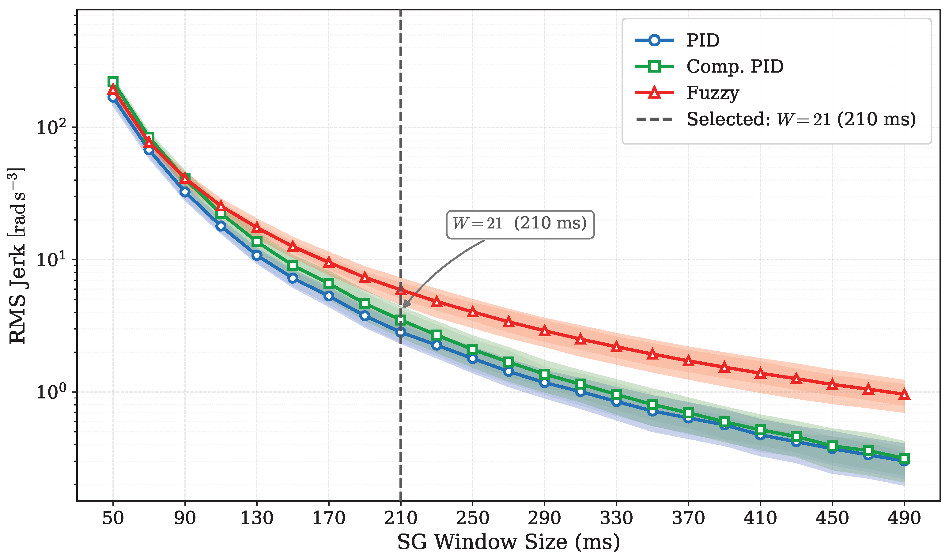
Figure 14 shows the evolution of the steady-state RMS-J as a function of the SG filter window length. Each point corresponds to the mean value obtained across all analyzed reference speeds, while the shaded regions represent the dispersion observed among experimental repetitions.

As expected, the RMS-J decreases systematically as the window length is increased. This behavior results from the progressive removal of components at high-frequency from the velocity signal, causing the estimated second derivative to approach lower values. For window lengths close to the minimum admissible value of the filter ($W=50$ ms), the effects of encoder quantization and measurement noise remain clearly observable.

The most relevant result, however, is that the relative differences among controllers persist even under substantial smoothing. As the window length increases, the jerk values of all three controllers gradually converge toward zero. Nevertheless, the fuzzy controller consistently exhibits higher RMS-J values than both the classical PID and the compensated PID. This tendency remains visible throughout the entire range of analyzed window lengths, including those for which the smoothing effect becomes dominant. Similarly, the compensated PID maintains RMS-J values slightly higher than those of the classical PID, although with a considerably smaller difference than that observed for the fuzzy controller.

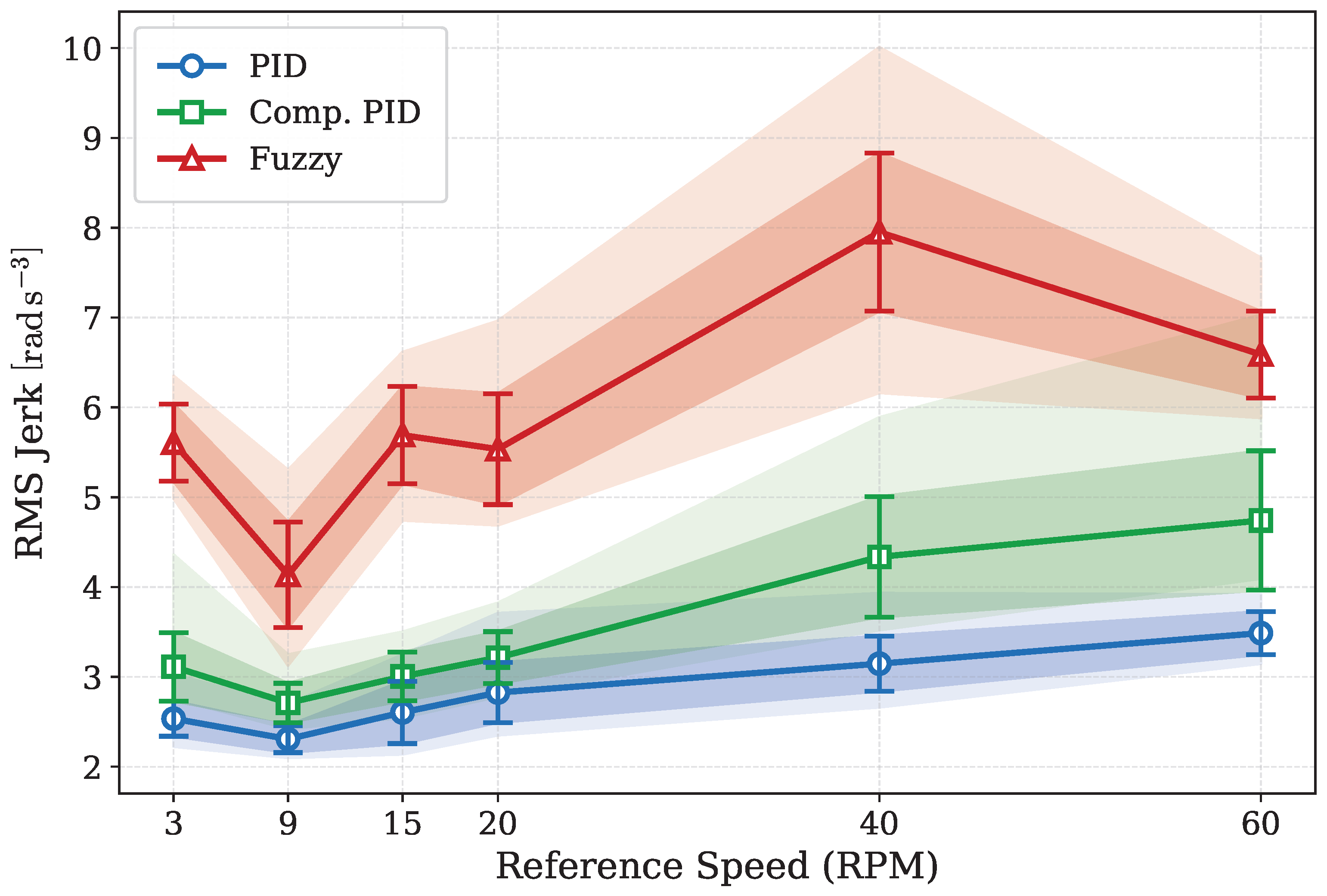
The relationship between RMS-J and reference speed was subsequently evaluated using the selected window length. The corresponding results are shown in Figure 15.

6.4. Kinematic Results Under Disturbance Conditions

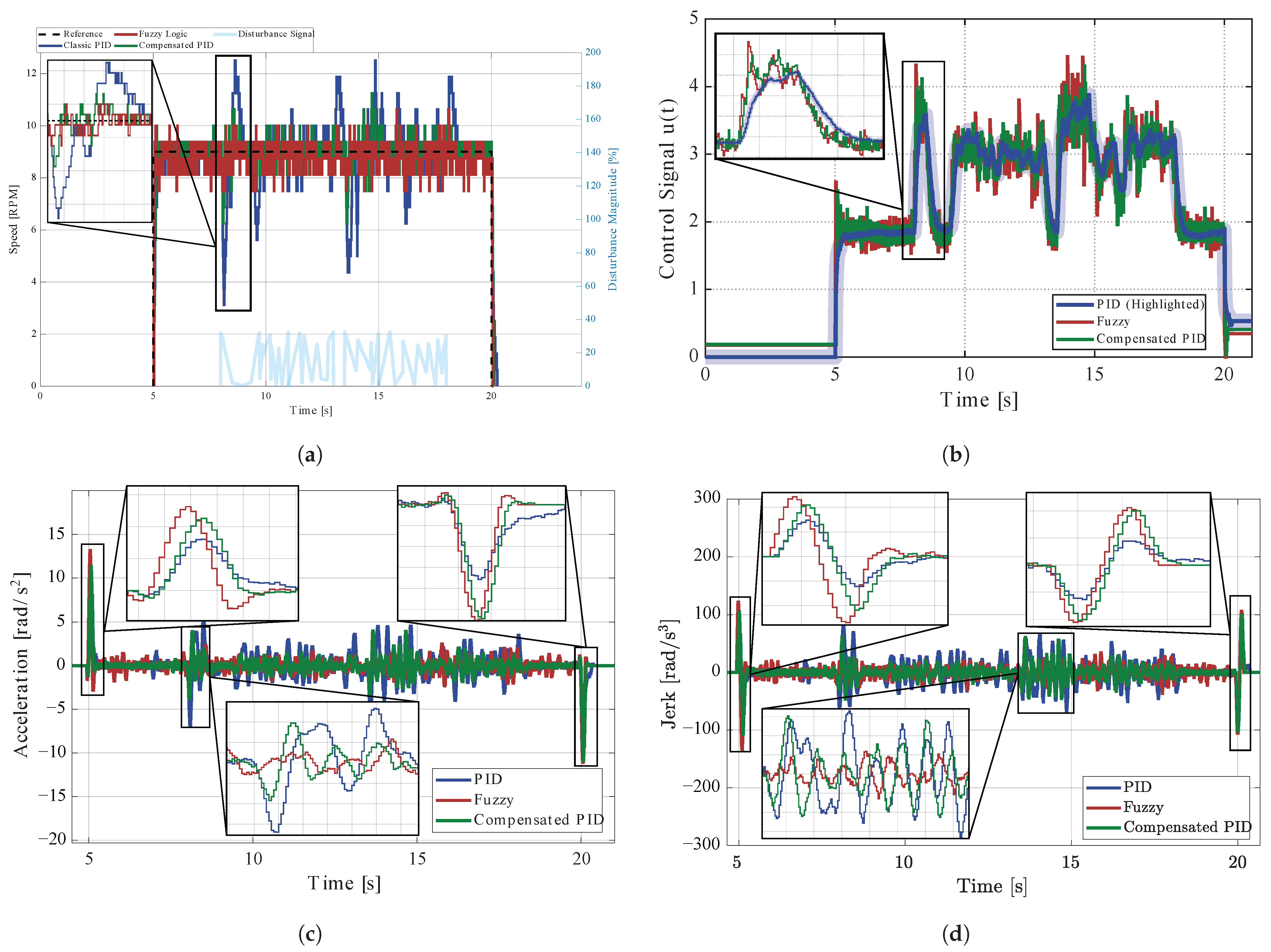
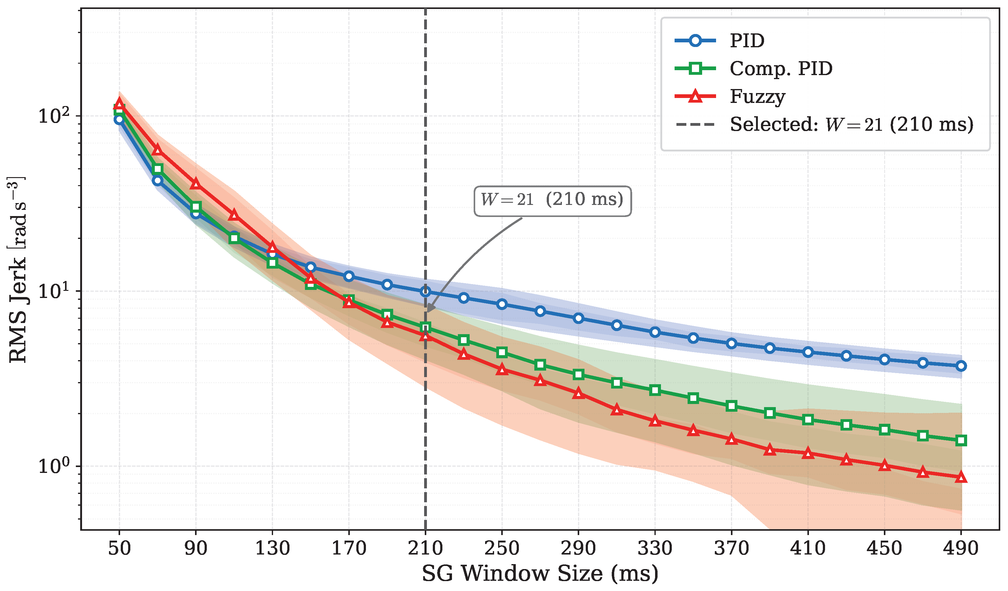
Figure 16 shows the evolution of the steady-state RMS jerk under mechanical disturbance conditions for different window lengths. For short windows (below approximately $130\mathrm{ms}$), the compensated PID and fuzzy controllers replicate the relative ordering observed in the unperturbed case, with the fuzzy controller presenting slightly higher RMS jerk than the compensated PID. At these scales, the contribution of encoder quantization variability is predominant. As the window length increases toward the crossing region (approximately 130–$170\mathrm{ms}$), the three curves converge and interchange their relative positions. Beyond this region, as the encoder noise contribution diminishes, a clearer ordering emerges: the fuzzy controller exhibits the lowest RMS jerk, followed by the compensated PID, while the classical PID presents the largest residual fluctuations across all larger window sizes.

This behavior suggests that each control strategy responds differently to disturbances depending on the temporal scale of analysis. For short windows, the fuzzy controller and the compensated PID replicate the same relative ordering observed in the unloaded case, indicating that the load does not fundamentally alter their high-frequency corrective behavior. The classical PID, conversely, presents the highest RMS jerk values across all window sizes, suggesting a consistently higher level of residual oscillation regardless of the analysis scale.

As the window length increases and the estimated jerk becomes progressively dominated by low-frequency components, the separation among the controllers becomes more pronounced. Under these conditions, the fuzzy controller exhibits the lowest residual fluctuations, followed by the compensated PID, while the classical PID presents the largest sustained deviations. This ordering suggests that both the fuzzy strategy and the compensated PID are more effective at attenuating the low-frequency disturbances introduced by the mechanical load, whereas the classical PID lacks sufficient corrective authority to suppress them.

These results also highlight an important limitation of RMS jerk as a comparative metric under disturbance conditions. Whereas jerk was primarily associated with mechanical smoothness in the unloaded scenario, the presence of external disturbances causes the metric to capture both the dynamics of disturbance rejection and the corrective action of the controller activity. Consequently, a lower RMS jerk does not necessarily imply superior tracking performance.

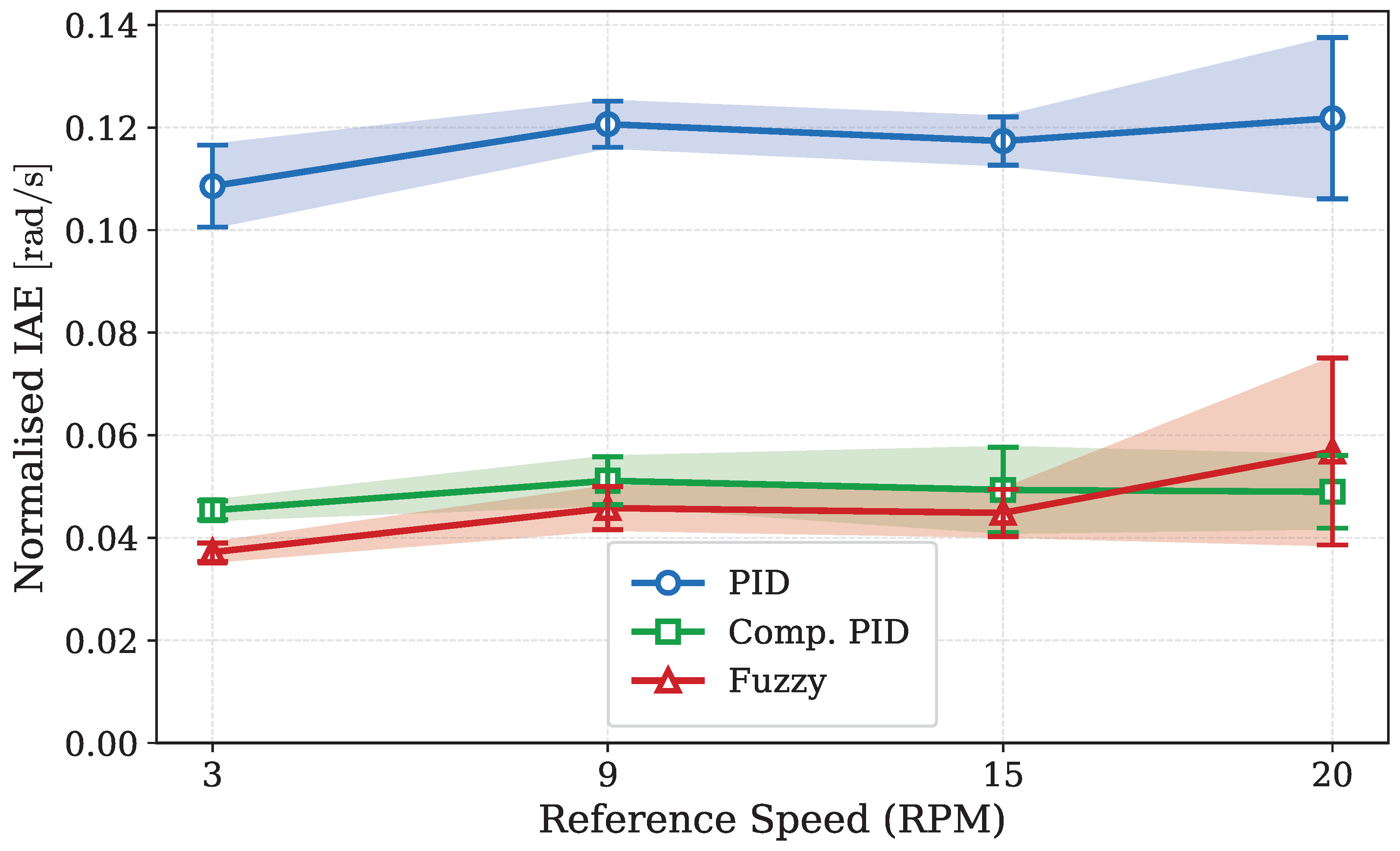
For this reason, a complementary metric based on the tracking error accumulated at steady state was incorporated. Figure 17 presents the normalized IAE obtained for each reference speed. Normalization was introduced to enable direct comparison across operating points, since the absolute value of the IAE naturally increases with the reference speed magnitude.

7. Discussion of Results

7.1. Analysis of Kinematic Profiles Without Disturbance

The first observation from Figure 14 is that, under no-load conditions, the fuzzy controller consistently exhibits the highest effective jerk magnitude in steady-state across all evaluated operating points. This behavior is quantified in

Table 7. RMS jerk at steady state under no-load conditions with the effect size of Kruskal–Wallis (W = 21 samples, order of SG filter = 3, Ts = 10 ms). Bold values indicate the lowest jerk at each speed.

Speed	Classic PID	Compensated PID	Fuzzy	${\widehat{\mathit{\eta }}}^2$
[RPM]	Jerk RMS [rad s−3]
3	2.535 ± 0.20	3.112 ± 0.38	5.608 ± 0.43	0.856
9	2.307 ± 0.15	2.710 ± 0.22	4.136 ± 0.59	0.833
15	2.605 ± 0.35	3.004 ± 0.27	5.691 ± 0.54	0.758
20	2.826 ± 0.33	3.215 ± 0.29	5.535 ± 0.62	0.771
40	3.147 ± 0.31	4.336 ± 0.67	7.950 ± 0.88	0.866
60	3.488 ± 0.24	4.741 ± 0.78	6.588 ± 0.48	0.841
Mean ± SD	$2.827\pm 0.484$	$3.498\pm 0.884$	$5.915\pm 1.302$

All Kruskal–Wallis tests: $p<0.001$ at every speed.

, computed with the SG window established in previous sections. Mean ± SD row represents the grand mean and between-speed standard deviation of the per-speed mean values.

The global statistics confirm a clear hierarchy: the classical PID achieves the lowest mean jerk RMS ($2.827\pm 0.484$ rad s⁻³), followed by the Compensated PID ($3.498\pm 0.884$ rad s⁻³), while the fuzzy controller produces approximately 1.7 times the jerk of its closest competitor ($5.915\pm 1.302$ rad s⁻³). The Compensated PID exhibits the highest coefficient of variation (CV = 25.3%), while the fuzzy controller also shows considerable variability (CV = 22.0%), both indicating lower repeatability than the classical PID (CV = 17.1%). This inferiority of the fuzzy controller is systematic: across all six evaluated operating points, it produces greater jerk than both competitors without exception, with a mean excess of 109.23% over the classical PID and 69.5% over the Compensated PID. The Kruskal–Wallis tests confirm that these differences are not only statistically significant ($p<0.001$ at all speeds) but also practically large, with effect sizes ${\widehat{\eta }}^2\in [0.76,0.87]$ indicating strong group separation across the entire operating range. With this quantitative context established, Figure 18 provides the complementary qualitative view of the four kinematic signals.

Figure 18a reveals velocity distortion peaks attributable to the fuzzy controller, while the Compensated PID exhibits oscillations of lower amplitude or excursions around the stability zone, also known as the deadband; the classical PID remains predominantly within this zone throughout steady-state operation, exhibiting very few fluctuations. This behavior has a structural explanation: the fuzzy controller bases its control decisions on an inference rule set that assigns corrective actions in response to any perceptible deviation in the error or its rate of change. In steady-state, where the residual error is small but nonzero, these rules continue to activate in response to velocity fluctuations that persist even after filtering. Although the filter attenuates high-frequency quantization jitter in the error signal, it does not eliminate the low-amplitude variations that occur at rates below its cutoff frequency, generating corrections that in a linear controller would be negligible. The observable result is precisely that pattern of intermittent spikes: the fuzzy mechanism reacts to variations that the classical PID, with its integral gain implicitly acting as a deadband, absorbs without producing any significant control action. The Compensated PID occupies an intermediate position between the conventional PID and the fuzzy controller. Although the compensation action increases sensitivity to error variations and promotes a more reactive response, its structure remains grounded in a linear control law based on the plant dynamic model. As a result, the controller is able to accelerate error correction relative to the classical PID without introducing the same level of control activity observed in the fuzzy strategy. This characteristic is reflected in the experimentally obtained RMS-J values, which remain systematically above those recorded by the conventional PID, yet significantly below those corresponding to the fuzzy controller.

Figure 18b further clarifies the causal mechanism described above. The control signal $v\left(t\right)$ of the fuzzy controller shows continuous variation of larger amplitude, a direct reflection of the fact that its inference rules produce perceptibly different control outputs in response to small oscillations of the steady-state error: when the error varies slightly, the active membership function shifts to a different region, and the defuzzified output undergoes a discrete jump that translates into a change in the voltage applied to the motor. This phenomenon, inherent to the discrete nature of the rule base, is the root cause of the velocity oscillations observed in panel (a) and, ultimately, of the higher jerk quantified in Table 7. The Compensated PID exhibits similar but attenuated variation, since its compensation acts on the error proportionally and continuously, without the jumps associated with defuzzification. The classical PID, by contrast, maintains a nearly constant control effort: operating with fixed gains over a small residual error, the control action converges to a stable equilibrium value, which accounts for both the absence of velocity spikes and its lower jerk values.

Figure 18c,d complete the analysis with the acceleration and jerk. During the transient phase, no meaningful distinctions in kinematic quality can be established, as all three controllers generate predictable acceleration and jerk profiles proportional to the tracking dynamics of each. In steady-state, however, the cumulative effect of the fuzzy mechanism’s discrete corrections becomes fully apparent: the continuous variations in $v\left(t\right)$ produce acceleration fluctuations that, upon differentiation, are amplified as jerk, giving rise to the elevated values quantified in Table 7. This result confirms that the fuzzy controller’s limitation in kinematic profiles is not attributable to a poor rule design for reference tracking, an area in which its performance is superior; instead, it stems from an inherent consequence of the implicit discretization in defuzzification, which prevents the maintenance of a sufficiently smooth control effort during steady-state regulation, and is consistent with greater mechanical loading on the actuator, suggesting elevated wear potential under sustained operation according to established jerk–fatigue relationships. From an engineering standpoint, the 109.23% higher steady-state RMS jerk produced by the fuzzy controller relative to the classical PID, (Table 7) translates into greater potential mechanical wear. According to the established motion planning literature, jerk is precisely the kinematic quantity that governs the excitation of residual vibrations and the accumulation of dynamic loads in mechanical transmission elements: smoother jerk profiles directly reduce both vibration residuals and surface fatigue rates [33,34]. Although a full frequency-domain vibration characterization is beyond the scope of the present work due to the requirement for dedicated chassis instrumentation, the jerk profile constitutes a well-established kinematic proxy for vibration excitation potential [33], suggesting that the fuzzy controller can be expected to impose a structurally higher mechanical cost during continuous operation, as exemplified by long duration terrain traversal.

7.2. Analysis of Kinematic Profiles Under Disturbance

The presence of load substantially modifies the relative ordering of the controllers compared to the undisturbed scenario. Figure 16 shows that the jerk RMS exhibits a marked frequency dependence. At narrow windows ($W\le 130$ ms), where encoder quantization variability dominates, the fuzzy and compensated PID controllers replicate the same relative ordering observed in the unloaded case, making it difficult to attribute differences exclusively to disturbance rejection. As the window widens and this quantization contribution diminishes, the controllers diverge: for $W\ge 210$ ms the classical PID becomes the worst performer, while the fuzzy and compensated PID converge toward significantly lower values. The physical mechanisms underlying this separation are examined through the kinematic profiles of Figure 19.

Table 8. Steady-state jerk RMS per velocity setpoint under mechanical load. Bold indicates best performer per speed.

Speed [RPM]	Classic PID	Compensated PID	Fuzzy	${\widehat{\mathit{\eta }}}^2$
3	$8.0562\pm 1.0327$	$5.2927\pm 0.8742$	$\mathbf{3}.\mathbf{9603}\pm \mathbf{0}.\mathbf{7877}$	0.77
9	$10.0518\pm 1.5948$	$5.6179\pm 0.8251$	$\mathbf{5}.\mathbf{0623}\pm \mathbf{2}.\mathbf{3454}$	0.60
15	$10.6859\pm 1.1927$	$6.2296\pm 2.2395$	$\mathbf{5}.\mathbf{3323}\pm \mathbf{1}.\mathbf{6460}$	0.57
20	$11.0861\pm 1.1754$	$\mathbf{7}.\mathbf{6623}\pm \mathbf{3}.\mathbf{0552}$	$7.9152\pm 3.6680$	0.27
Mean ± SD	$9.9700\pm 1.3450$	$6.2006\pm 1.0490$	$\mathbf{5}.\mathbf{5675}\pm \mathbf{1}.\mathbf{6738}$

All Kruskal–Wallis tests: $p\le 0.011$.

and

Table 9. Normalized IAE per velocity setpoint under mechanical load. Bold indicates best performer per speed.

Speed [RPM]	Classic PID	Compensated PID	Fuzzy	${\widehat{\mathit{\eta }}}^2$
3	$0.1086\pm 0.0080$	$0.0454\pm 0.0019$	$\mathbf{0}.\mathbf{0372}\pm \mathbf{0}.\mathbf{0018}$	0.88
9	$0.1206\pm 0.0045$	$0.0511\pm 0.0047$	$\mathbf{0}.\mathbf{0458}\pm \mathbf{0}.\mathbf{0042}$	0.73
15	$0.1174\pm 0.0047$	$0.0493\pm 0.0083$	$\mathbf{0}.\mathbf{0449}\pm \mathbf{0}.\mathbf{0046}$	0.69
20	$0.1218\pm 0.0157$	$\mathbf{0}.\mathbf{0490}\pm \mathbf{0}.\mathbf{0071}$	$0.0568\pm 0.0182$	0.66
Mean ± SD	$0.1171\pm 0.0060$	$0.0487\pm 0.0024$	$\mathbf{0}.\mathbf{0462}\pm \mathbf{0}.\mathbf{0081}$

All Kruskal–Wallis tests: $p<0.001$.

summarize both metrics at the selected window. The fuzzy controller achieves the lowest global jerk RMS and the lowest normalized IAE, with reductions of approximately 44% and 61%, respectively, relative to the classical PID. The compensated PID follows closely, with reductions of 38% in jerk RMS and 58% in IAE. Effect sizes for IAE (${\widehat{\eta }}^2\in [0.66,0.88]$) remain consistently larger than those for jerk RMS (${\widehat{\eta }}^2\in [0.27,0.77]$), confirming that tracking error is the more discriminative metric under disturbance. The notably weaker effect at 20 RPM for jerk RMS (${\widehat{\eta }}^2=0.27$) reflects the reduced mechanical perturbation at that operating point.

Dunn post hoc comparisons with Bonferroni correction confirm that the classical PID differs significantly from both the compensated PID and the fuzzy controller at all speed setpoints for both metrics. By contrast, the compensated PID and fuzzy controller do not differ significantly in jerk RMS at any speed. For IAE, a significant difference between them is detected only at 3 RPM ($p=0.033$), with the fuzzy controller outperforming the compensated PID; at higher speeds no significant difference is found.

Figure 19 illustrates the physical mechanisms underlying these results across the four kinematic signals.

Figure 19a reveals the most critical effect of the disturbance on the classical PID: in response to velocity drops coinciding with the dominant frequency of the load signal ($f_{\mathrm{dom}}=0.78$ Hz), the controller fails to react quickly enough and the velocity falls abruptly, producing sustained deviations from the reference. This sluggish response is a direct consequence of its fixed-gain linear structure: the corrective action is strictly proportional to the instantaneous error and its derivative, which means that under a sudden torque disturbance the controller can only recover gradually, accumulating tracking error throughout the perturbation cycle. This phenomenon is the direct cause of its elevated IAE and the high RMS of the jerk at low frequency: the tracking error is real and sustained, not a spectral artifact.

The fuzzy controller, by contrast, reacts more rapidly to these nonlinear disturbances by virtue of its inference rule structure. When the velocity error and its rate of change simultaneously become large as occurs during a load-induced drop multiple rules fire concurrently and produce a disproportionately large corrective output that a fixed-gain controller cannot replicate. This nonlinear amplification of the control action in critical regions is what allows the fuzzy controller to arrest the velocity deviation before it accumulates significantly. The compensated PID achieves a similar effect through its model-based feedforward term, which partially anticipates the disturbance and supplements the feedback correction; however, its linear gain structure limits its adaptability compared to the inference-based strategy. Both controllers therefore generate continuous high-frequency corrections, as shown in Figure 19b, which explains their higher jerk RMS at narrow windows but their superior overall tracking performance.

At 20 RPM, the compensated PID presents slightly lower values than the fuzzy controller in both metrics; although this reversal does not reach statistical significance, it is consistent with the model-based structure of the compensated PID providing marginally more effective load rejection at the upper end of the operating range, where the disturbance torque is relatively larger with respect to the available motor output.

Figure 19c,d confirm that the most significant differences among controllers are concentrated in the steady-state region under disturbance, where the effective jerk peaks are considerably larger than in the undisturbed scenario. This increase reflects the more aggressive kinematics imposed by the disturbance, and its magnitude is consistent with the values reported in Table 8 and Table 9.

From a durability standpoint, the sustained jerk peaks generated by the classical PID under disturbance, up to 2.0 times higher than those of the fuzzy controller, are consistent with cyclically applied force reversals that, according to the established fatigue literature [34], are expected to contribute to accelerated fatigue in the coupling and bearing assembly, suggesting that the classical PID may be less suitable for continuous loaded operation.

8. Conclusions

This study experimentally compared three strategies for speed control in a PMDC rover actuator implemented on an RP2040 microcontroller: a classical PID, a compensated PID, and a Mamdani fuzzy controller. Across all operating conditions, statistically significant differences were observed in both conventional tracking metrics and kinematic indicators, demonstrating that controller selection strongly influences not only tracking accuracy but also the kinematic loading profile of the actuator, with potential implications for mechanical wear.

8.1. Main Technical Findings

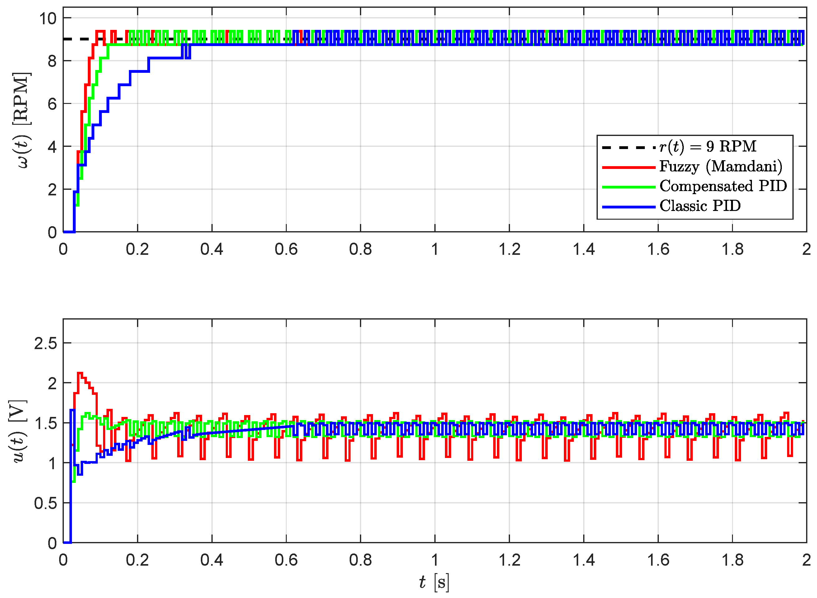
The results reveal that controller performance depends strongly on operating conditions. Under nominal conditions, the classical PID produced the smoothest motion, achieving a mean jerk RMS less than half that of the fuzzy controller, which exceeded the classical PID by 109.23% and the compensated PID by 69.5% across all evaluated speeds. Under mechanical disturbance, however, the performance hierarchy inverted substantially: the fuzzy controller reduced jerk RMS and normalized IAE by 44% and 61%, respectively, relative to the classical PID, while the compensated PID provided reductions of 38% and 58%. These findings indicate that a controller optimized for kinematic smoothness under nominal operation is not necessarily the most effective strategy when sustained disturbances are present.

8.2. Principal Contribution

The principal and novel contribution of this work is threefold. First, a jerk-based kinematic evaluation framework is proposed and validated experimentally for embedded speed controllers operating under quantized encoder measurements, including a principled Savitzky–Golay filter selection methodology. Second, it is demonstrated that the kinematic performance hierarchy undergoes a complete inversion between nominal and disturbed conditions—a reversal statistically confirmed across repeated trials and multiple operating speeds, and entirely invisible under classical transient metrics such as rise time, settling time, and integral error. Third, the engineering significance of this inversion is established: the controller producing the smoothest kinematic profile under nominal operation simultaneously generates the highest mechanical loading under variable loads, with potential implications for actuator durability, consistent with established jerk fatigue relationships in the literature [37].

8.3. Engineering Recommendations

From an engineering perspective, the results suggest that the classical PID remains an attractive solution for applications operating predominantly under nominal conditions, whereas the fuzzy and compensated PID controllers provide superior robustness when disturbance rejection is required. Consequently, kinematic indicators should be considered alongside traditional control metrics when selecting controllers for electromechanical systems subject to variable loading.

8.4. Limitations

The conclusions of this study are restricted to step-reference tracking and the controlled disturbance profiles evaluated in the experimental platform. Furthermore, the analysis focuses on actuator kinematics and does not include direct vibration measurements or long-term wear characterization. Consequently, the observed relationships between jerk and potential mechanical degradation should be interpreted as indirect indicators supported by the existing literature rather than direct measurements. Finally, the fixed-window velocity estimation introduces jitter that, although reducible via interrupt-based period measurement on the RP2040, was deliberately retained to reflect the sensing constraints of less capable microcontrollers.

8.5. Future Work

Future work should address two open research directions. First, the present study deliberately employs step references and controlled braking disturbances as a methodologically controlled baseline to isolate the effect of each control strategy on the kinematic response. While this choice enables clean comparative analysis, extending the evaluation framework to ramp references and terrain-induced disturbances such as those arising from obstacle negotiation or surface transitions on the PRAXIA rover would broaden the applicability of the proposed methodology to more realistic operational scenarios and strengthen its practical relevance for autonomous navigation applications. Second, evaluating hybrid strategies for speed measurement, such as methods that mix frequency and period, could further reduce the constraint on quantization imposed by the fixed-window approach adopted here.