Spectrum-Aware Generative Model for Small-Sample Motor Fault Diagnosis

Abstract

This paper proposes a spectrum-aware generative learning framework for intelligent motor fault diagnosis under small-sample conditions. To address the challenges of insufficient labeled fault data and imbalanced distributions in motor systems, a hybrid model integrating a generative adversarial network (GAN) with an attention-enhanced deep neural network is developed. First, vibration signals of the motor are transformed into time–frequency representations to capture discriminative spectral features. Then, the GAN is employed to augment minority classes and improve data diversity, while the SE (squeeze-and-excitation) mechanism enhances feature extraction by emphasizing critical fault-related components. Finally, a deep classifier is trained on the augmented dataset for fault identification. Experimental results on benchmark datasets demonstrate that the proposed method achieves superior diagnostic accuracy and robustness compared with several state-of-the-art approaches, especially under severe data scarcity and imbalance scenarios. The results indicate that the proposed framework effectively improves generalization performance and provides a reliable solution for intelligent motor fault diagnosis in practical industrial applications.

1. Introduction

The motor is a complex system coupled by multiple physical fields, such as electric and magnetic fields [1]. It is widely applied in industries, agriculture, transportation, national defense, and daily life [2,3]. With the rapid advancement of industrial automation and intelligent manufacturing, the demand for efficient and accurate fault diagnosis systems has grown significantly, particularly in the early detection of potential failures and the prevention of unexpected downtime [4,5]. However, conventional motor fault diagnosis approaches largely rely on one-dimensional time and frequency domain features and signal analysis techniques, which often struggle under non-stationary, nonlinear, and noise-intensive operating conditions [6,7]. Meanwhile, their diagnostic accuracy will be further reduced because of insufficient data and the easy overfitting of deep learning models, which limits their applicability in modern industrial environments requiring real-time and intelligent solutions [8,9,10]. Therefore, investigating motor fault diagnosis under small-sample data conditions, combining image representation with deep learning classifiers, is crucial for improving fault detection efficiency and enhancing the operational robustness of motor systems [11,12,13].

In recent years, significant advances have been achieved in fault diagnosis through the integration of time-series-to-image transformations and deep neural networks. On the one hand, recursive plot (RP), Gramian angular field (GAF), and Markov transfer field (MTF) are widely used to convert the original one-dimensional vibration signal into a two-dimensional representation, which can more richly characterize the time pattern and structural correlation. For instance, Xu developed a method that combines block 2D principal component analysis with a depth-separable convolutional model, demonstrating enhanced performance in rolling bearing fault identification [14]. More recently, Zhao proposed a multi-source information fusion approach that has integrated time-frequency image representations with one-dimensional convolutional neural networks (CNNs) features, achieving nearly 99% diagnostic accuracy and high generalization across datasets [15]. Similarly, Zhang discussed the application of deep learning in bridge health monitoring, emphasizing its adaptability and transferability in complex engineering systems [16]. Multidisciplinary applications also suggest the potential of deep learning combined with spectral imaging for fast identification tasks, as demonstrated by Raman spectroscopy-based bacterial detection [17]. Despite these advances, data scarcity remains a major bottleneck in motor fault diagnostics. To address this challenge, transfer learning, generative adversarial networks (GANs), and their variants, such as DCGAN and Wasserstein generative adversarial networks (WGANs), have been extensively studied. With architectural refinements and spectral regularization strategies, these models further improve the reliability of classification under small sample scenarios [18]. In order to solve the problem of the GAN suffering from mode collapse or unstable sample quality under extremely limited data conditions. A variety of enhanced architectures have been proposed: for instance, an enhanced GAN demonstrated improved performance for the imbalanced fault diagnosis of rotating machines [19]; the modified conditional generative adversarial network (MCGAN), based on memristive hyperchaotic sequences and a mixed-dimensional convolutional neural network (MCNN), was proposed for augmenting the fault sample and reducing the imbalanced rate [20]; and the residual signal-driven GAN integrating dual-stream attention was reported to extract the fault characteristics of induction motors [21]. Furthermore, hybrid approaches combining DCGANs with CNNs have been successfully applied to permanent magnet motor diagnosis under small sample settings [22]. The improved DCGAN and Gramian Angular Summation Field (GASF) methods have been applied to arc fault diagnosis of photovoltaic arrays [23]. Although standard deep convolutional networks have shown strong feature extraction capabilities, such networks usually give equal weight to all extracted feature channels. In the actual industrial scene, the signal is often accompanied by strong background noise, and not all the extracted frequency features have the same fault diagnosis value. Consequently, combining spectral constraints for high-quality data augmentation with architectures that capture both local details and global dependencies remains a critical direction for future research in Motor fault diagnosis. This is the first motivation of this study.

With the development of neural networks, CNNs and their variants have been widely recognized as powerful tools for fault diagnosis [24]. Wen proposed a data-driven CNN-based framework that demonstrated superior feature extraction capability compared with traditional signal processing approaches, laying the groundwork for end-to-end diagnostic models [25]. Building upon CNNs, residual networks (ResNets) were introduced to overcome the gradient disappearance problem in the deep structure, making the learning of hierarchical fault features more robust. For example, fault diagnosis strategies using ResNet have been successfully applied to driving motor diagnostics, significantly enhancing recognition accuracy under limited data conditions [26]. The auxiliary classifier generative adversarial network (GAN), which incorporates convolution and transformer modules, realizes the extraction of global and local features and improves the classification accuracy [27]. Similarly, dual-mode attention-based residual architectures have been developed to capture both the spatial and temporal dependencies of vibration signals, thereby achieving improved adaptability under variable operating conditions [28]. In addition, recent systematic reviewshave highlighted the growing role of CNNs and ResNets as mainstream architectures for fault diagnosis, emphasizing their capacity to generalize across diverse machinery and fault scenarios [29,30]. Overall, CNNs and ResNet-based models provide strong foundations for designing diagnostic frameworks, but their effectiveness is still closely tied to data sufficiency and model generalization, motivating the integration with generative and attention-based mechanisms in recent research. This gives us a clear research direction.

Although substantial progress has been achieved in fault diagnosis through time series-to-image conversion and deep neural network classification, several key challenges remain unresolved. First, most image transformation techniques fail to incorporate spectral characteristics adequately, resulting in limited sensitivity to frequency domain information of the fault signals. Second, in terms of model architecture, the integration of local features with long-range dependencies is still insufficiently explored. At the same time, more research is needed to design diagnostic networks with stronger representational capability. Based on the above discussion, we study spectrum-aware generative models based on RP. Using RP retains the complete time dependence and reduces the sensitivity to random noise. When combined with DCGAN, it is used to generate high-quality samples and achieve sample balance. The RP spatial layout in the image has time delay and topological symmetry, rather than physical shape. Spatial attention processing is easily misguided; this urgently needs an attention method for the channel level. This particular need constitutes the core motivation for us to choose the SE mechanism. Different from spatial attention, the SE mechanism explicitly models the dependencies between channels to achieve adaptive feature recalibration, thereby dynamically amplifying specific channels containing key mechanical failure frequencies and suppressing noise-dominated channels. The improved DCGAN-ResNet-SE model for motor fault diagnostics is proposed and verified on mechanical faults and electrical faults, such as motor bearing faults and stator inter-turn short circuit faults. The main contributions are as follows.

(1)

A spectrum-aware generative learning framework is proposed for intelligent motor fault diagnosis under small-sample conditions. By incorporating frequency-domain consistency constraints into the adversarial training process, the proposed method effectively improves the quality and reliability of generated samples, thereby alleviating the data scarcity problem in practical industrial systems.

(2)

A spectrum-aware filtering and feedback mechanism is developed to evaluate the similarity between generated samples and real signals in the frequency domain. The screening strategy selectively retains high-quality synthetic samples and reinjects them into the adversarial training loop, forming a closed-loop optimization process that enhances both the stability and diversity of the generated data.

(3)

An attention-enhanced deep classification network based on ResNet is designed to improve diagnostic performance. By integrating the SE mechanism with residual learning, the proposed model captures both local transient features and long-range dependencies in vibration signal representations, leading to more robust fault identification under limited data conditions.

The remainder of this paper is organized as follows: Section 1 introduces the research background, motivation, and contributions; Section 2 reviews the theoretical background; Section 3 presents the proposed spectrum-aware DCGAN with dynamic threshold filtering in detail; Section 4 reports the experimental setup and results; and Section 5 concludes the paper and discusses future research directions.

2. Theoretical Background

2.1. Recurrence Plot

Recurrence Plot (RP) [31] is a technique used to visualize the dynamics of time series data. By transforming a one-dimensional signal into a two-dimensional representation, RP highlights temporal patterns and structural correlations. Given a signal sequence $X=\left\{x(1),x(2),x(3),\dots ,x(N)\right\}$, the reconstructed state vectors with a time delay can be expressed as.

$$X(i)=[x(i),x(i+\tau ),\cdots ,x(i+(m-1)\tau )]$$

(1)

where $i=1,2,\dots ,N-(m-1)$, $\tau$ denotes the delay time and $m$ is the embedding dimension. The optimal values of $\tau$ and $m$ are typically determined using the autocorrelation function method.

The distance between any two vectors in the reconstructed phase space is evaluated.

$$D_{ij}=\Vert X_i-X_j\Vert$$

(2)

Based on these distances, the recurrence matrix of the phase space can be defined as.

$$R_{ij}=\mathrm{\Theta }(\epsilon -D_{ij})$$

(3)

where $\epsilon$ is a threshold for recurrence, commonly chosen as approximately 15% of the standard deviation of the original series.

2.2. Generative Adversarial Network

GANs [32] are a class of generative models with two core components: a generator G and a discriminator D, trained simultaneously in an adversarial manner. The generator samples from a latent space and produces data resembling the distribution of real samples, while the discriminator determines whether the input comes from the true dataset or is created by the G. During training, the G improves its ability to “fool” the D, while the D enhances its ability to distinguish real from synthetic data.

Mathematically, the training objective of a GAN is a minimax optimization problem:

$$\begin{array}{r}{\min }_G{\max }_{D}V(D,G)={\mathbb{E}}_{x~p_{\mathrm{data}}(x)}[\log D(x)]\\ +{\mathbb{E}}_{z~p_z(z)}[\log (1-D(G(z)))]\end{array}$$

(4)

where x denotes real data from the distribution $p_{\mathrm{data}}(x)$, and $p_z(z)$ is the prior noise distribution. The operator $\mathbb{E}$ denotes the expectation, and G(z) represents synthetic samples produced by the generator.

A key advantage of GANs is their ability to learn complex data distributions without requiring explicit probability density modeling. However, the non-convex nature of the minimax game leads to instability or mode collapse. To address this, architectures like Deep Convolutional GANs (DCGANs) and Wasserstein GANs (WGANs) improve sample quality and convergence stability.

2.3. Deep Convolutional GAN

In the conventional GAN framework, both the generator and discriminator are typically implemented using fully connected layers. However, such architectures are prone to excessive parameterization when handling high-dimensional image data, leading to inefficient training and difficulty in preserving spatial structures in the generated samples. To overcome these drawbacks, Radford et al. introduced the Deep Convolutional GAN (DCGAN) [33], which incorporates convolutional neural network architectures to enhance both spatial consistency in generation and discriminative capability in classification.

In the generator, DCGAN employs transposed convolution layers to progressively map the low-dimensional latent vector $z\sim p_z(z)$ into high-dimensional images. Formally, the mapping process can be expressed as.

$$x_g=G(z)=f(W_g\ast z+b_g)$$

(5)

where $*$ denotes the transposed convolution operation, $W_g$ and $b_g$ are the generator parameters, and $f(\cdot )$ is generally a ReLU or Leaky ReLU activation. This hierarchical expansion allows the model to increase the resolution of feature maps step by step, producing images with meaningful local spatial structures.

For the discriminator, DCGAN leverages conventional convolution and down-sampling layers to compress the input image progressively, extracting features that are discriminative between real and generated samples. Its discriminative function can be written as.

$$D(x)=\sigma (W_d*x+b_d)$$

(6)

where $\sigma (\cdot )$ represents the sigmoid activation function, outputting the probability that the input image belongs to the real data distribution.

Through these architectural innovations, DCGAN demonstrates significantly more stable convergence than the original GAN and generates images with superior visual quality and structural fidelity. These advantages not only enhance training stability and sample realism but also establish DCGAN as a widely adopted data augmentation technique for addressing small sample challenges in fault diagnosis of rotating machinery.

2.4. Convolutional Neural Network

CNNs are a category of deep learning models characterized by local connectivity, shared parameters, and hierarchical feature extraction capabilities. Compared with traditional fully connected neural networks, CNNs can significantly reduce the number of parameters when processing images, audio, or time-series signals, while more effectively capturing local spatial correlations. In the context of mechanical fault diagnosis, vibration signals transformed into images typically exhibit two-dimensional textures with temporal patterns. CNNs are capable of progressively extracting multi-level features from these representations, ranging from low-level edge textures to high-level semantic patterns. The primary components of a CNN include convolutional layers, activation layers, pooling layers, and fully connected layers.

Although CNNs excel in feature extraction, increasing network depth can lead to issues such as vanishing gradients or performance degradation, where the model’s accuracy may actually drop beyond a certain number of layers. To address this problem, He proposed the Residual Network (ResNet) [34].

The key innovation of ResNet is residual learning. By introducing identity-based skip connections, ResNet allows a deep network to directly learn the residual mapping between the input and output.

$$y=F(x,W)+x$$

(7)

where $F(x,W)$ represents a nonlinear transformation composed of convolutional layers and activation functions, $x$ is the input feature, and $y$ is the output feature.

This design ensures that, although $F(x,W)$$F(x,W)$ learns an effective mapping, the network can still preserve identity mapping, thus avoiding degradation.

2.5. SE Mechanism

In deep convolutional neural networks, the contribution of each extracted feature channel to the final classification result varies. Traditional convolutional mappings treat all channels with equal weight, which limits the discriminative power of the model in fault diagnosis scenarios characterized by significant background noise. To address this, the SE (squeeze-and-excitation) mechanism [35] is introduced in this study to model the inter-dependencies between channels and achieve adaptive feature recalibration. The SE module primarily consists of two key processing units: squeeze and excitation.

Squeeze Unit: This unit aims to compress spatial information into channel descriptors. Given an input representation $X\in {\mathbb{R}}^{H\times W\times C}$, a global average pooling mapping is employed to compress the $H\times W$ spatial features of each channel into a single global descriptive value $z_c$.

$$z_c={\displaystyle \frac{1}{H\times W}}{\displaystyle \sum _{i=1}^H{\displaystyle \sum _{j=1}^W{x}_c}}(i,j)$$

(8)

where $x_c$ denotes the feature mapping of the $c$ channel.

This operation enables the model to obtain a global receptive field and capture the global distribution of features across all channels.

Excitation Unit: This unit captures non-linear dependencies between channels through two fully connected layers. To reduce the parameter count, a dimensionality reduction weight matrix $W_1$ is first applied, followed by a dimensionality recovery weight matrix $W_2$ to return to the original channel dimension.

$$s=\sigma (W_2\cdot \mathit{ReLU}(W_1\cdot z))$$

(9)

where $\sigma$ represents the Sigmoid activation function, which maps the output to a weight coefficient $s$ ranging from 0 to 1.

Feature Recalibration: Finally, the generated weight coefficients are applied to the corresponding channels of the original feature map $X$ to perform feature reconstruction:

$${\tilde{x}}_c=s_c\cdot x_c$$

(10)

This channel-wise attention mechanism allows the model to autonomously learn the importance of different fault feature channels. In the context of fault diagnosis, the integration of the SE mechanism enables the network to reinforce feature channels sensitive to fault types (such as periodic textures in recurrence plots) while suppressing invalid channels affected by environmental noise. Consequently, this significantly improves the recognition accuracy and robustness of the model under complex operating conditions.

3. Improved DCGAN-ResNet-SE Model for Motor Fault

3.1. Improved DCGAN Algorithm Based on Spectrum-Aware Filtering

To further improve the quality of synthetic samples and ensure their physical plausibility in the frequency domain. A spectrum-aware filtering module is integrated into the training loop. The design theory of this module is strictly rooted in the physical nature of rotating machinery faults, and on this basis, the mathematical measurement method is optimized. At the advantage level of mathematical measurement, the traditional signal similarity evaluation often depends on the L1 Manhattan distance or the L2 Euclidean distance norm. However, these two spatial distance measures are extremely sensitive to signal phase offset and random ambient noise. Even in the frequency domain, due to the change in motor load under multiple operating conditions, the absolute amplitude of the spectrum induced by the same physical fault will fluctuate violently, resulting in the failure of the L1/L2 distance in evaluating sample fidelity. In contrast, the Pearson correlation coefficient used in this module is mainly used to measure the linear correlation between two vectors. Combined with the fast Fourier transform, this measurement method can effectively ignore the overall amplitude scaling and phase difference caused by the change in working conditions and focus on evaluating the high consistency between the generated samples and the real samples in the spectral contour. This screening mechanism, based on spectral contour similarity, forces the generator to learn the frequency distribution of faults mathematically, thus ensuring that the retained synthetic samples truly reproduce the resonance band structure of the corresponding faults in the physical principle, providing high-quality data support with high physical interpretability for subsequent classification models.

Specifically, every 10 epochs, the generator produces 100 candidate images, which are compared with reference samples from the minority class. Each candidate is converted into grayscale and transformed via a two-dimensional FFT. The magnitude spectrum is then logarithmically scaled, and the Pearson correlation coefficient is computed against the spectra of reference samples. For each candidate, the maximum correlation score is taken as its similarity measure. Samples with similarity exceeding a dynamic threshold ${\tau }_t=\min (0.25,; 0.10 + 0.01\times t/10)$ are retained, while others are discarded. To prevent overly strict filtering, a minimum-keep rule is applied: at least K_min = 5 candidates are preserved by selecting the top-ranked samples. All retained images are stored and iteratively fed back into the training process, providing high-quality synthetic data that enhances both the diversity and reliability of the classifier under limited-sample conditions. The procedure is as follows.

Candidate Sample Generation: At the end of each training iteration, the generator G produces a batch of candidate image samples.

$${\left\{x_g^i\right\}}_{i=1}^N$$

(11)

Spectral Mapping and Similarity Computation: Each candidate sample is transformed via an FFT to obtain its spectral representation.

$$\mathcal{F}(x_g^i)=\mathrm{FFT}(x_g^i)$$

(12)

is compared with the spectrum $\mathcal{F}(x_r)$ of the real reference sample to define the normalized spectrum difference.

$$d_i={\displaystyle \frac{\parallel \mathcal{F}(x_g^i)-\mathcal{F}(x_r){\parallel }_2}{\parallel \mathcal{F}(x_r){\parallel }_2}}$$

(13)

Dynamic threshold filtering: Set a gradually tightening spectral similarity threshold, whose value decreases with increasing training epochs t.

$${\tau }_t=\min \left({\tau }_{\max },\hspace{0.33em}{\tau }_0+\lambda \cdot t\right)$$

(14)

where ${\tau }_t$ represents the Sigmoid activation function, which maps the output to a weight coefficient ${\tau }_t=\min \left({\tau }_{\max },\hspace{0.33em}{\tau }_0+\lambda \cdot t\right)$ ranging from 0 to 1.

Feedback and closed-loop optimization: Selecting qualified samples is not only used to expand the training set of the classifier but also included as input for the next round of adversarial training, optimizing the discriminator on the joint distribution of real samples and high-quality generated samples, and gradually converging the generator towards spectral consistency. Its new adversarial objective can be expressed as.

$$\begin{array}{r}{\min }_G{\max }_D{V}^{\prime }(D,G)=E_{x~p_{data}(x)\cup p_{spec}(x)}\left[\log D(x)\right]\\ +E_{z~p_z(z)}\left[\log (1-D(G(z)))\right]\end{array}$$

(15)

where p_spec(x) represents the distribution of high-quality generated samples after spectral screening. The algorithm flowchart is shown in Algorithm 1.

Algorithm 1. Adversarial Training with Spectrum-Aware Filtering

Require: Training data X, reference set Xr, noise distribution $\mathcal{N}$ (0, I) Ensure: Best generator G*    1: Initialize generator G, discriminator D, optimizers;    2: for epoch = 1 to T do    3:   for each mini-batch of size B do    4:       Sample noise Z ~ $\mathcal{N}$ (0, I);    5:       Generate fake samples X^ = G(Z);    6:       Update discriminator D with real X and fake X^;    7:       Update generator G using discriminator feedback;    8:   end for    9:   if t mod fs = 0 then     10:      Sample candidate noise Zc;     11:      Generate candidate set $X_c^{^}$ = G(Zc);     12:      Compute FFT spectra and correlation with reference set Xr;     13:      Select samples with similarity s($X_c^{^}$) ≥ τi;     14:      if number of selected samples < kmin then     15:         Keep top-kmin most similar candidates;     16:      end if     17:      Save selected samples and metadata;     18:    end if     19: end for     20: return best generator G*

3.2. Classification Model Based on ResNet-SE

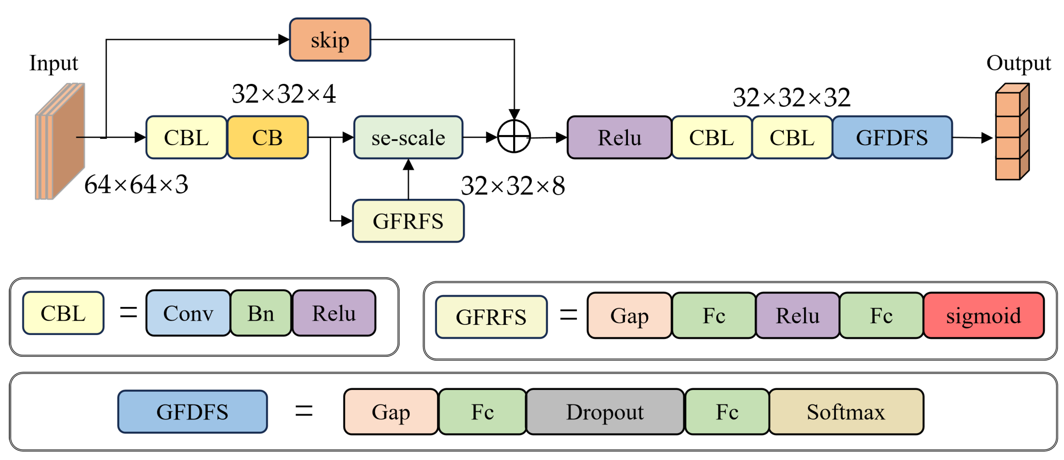
The ResNet-SE classification model constructed in this study builds upon a conventional CNN by integrating residual connections, feature concatenation, and the SE mechanism to achieve a high-precision classification of the fault signals. In technical diagnosis, vibration signals are often accompanied by strong environmental noise. This model realizes the compression and extraction of key features through the SE mechanism. Specifically, the input features are compressed by global average pooling, and the spatial information is transformed into a global channel descriptor. This topology compression mechanism enables the network to ignore invalid background noise and give higher weights to the feature channels containing periodic fault pulses, thus establishing a direct mapping between mathematical reconstruction and physical diagnosis. The network architecture primarily consists of an input layer, dual-branch feature extraction paths, a feature fusion module, convolutional and pooling layers, fully connected layers, and an attention mechanism, with a final Softmax layer for classification. The overall structure is illustrated in Figure 1 below.

Input Layer: Accepts color images of size 64 × 64 × 3, which represent the visualized vibration signals. This layer provides the raw information necessary for subsequent feature extraction.

Main Path: Uses a 4 × 4 convolutional layer to perform initial feature extraction on the input images, producing four output channels. The convolution is followed by batch normalization (BN) and ReLU activation to accelerate training convergence and enhance nonlinear feature representation. The 3 × 3 maximum pooling layer is used for spatial down sampling to reduce the feature dimension and improve the feature compactness while maintaining significant information.

Residual Path: To preserve essential input information and facilitate gradient propagation, a parallel residual branch is established. This branch employs a 1 × 1 convolution to adjust the channel dimensions, ensuring compatibility with the main path output. The residual features are later fused with the main path features during the feature concatenation stage, enriching feature representation and mitigating gradient vanishing issues.

Feature Concatenation Layer: Outputs from the main and residual paths are merged to form dual-channel features. The fused features then pass through multiple layers of convolution, batch normalization, ReLU activation, and pooling. The second convolutional layer outputs 16 channels, and the third convolutional layer outputs 32 channels. This hierarchical convolution and normalization process enables the model to progressively extract multi-scale fault features, from shallow texture to deep semantic patterns.

Fully Connected and SE Layer: After convolutional feature extraction, a flattening layer is employed to reshape the multi-dimensional feature maps, ensuring that the data format is compatible with the subsequent fully connected mapping and processing units. A 24-dimensional fully connected layer is then used for feature compression and combination. Subsequently, the SE mechanism is applied to perform an adaptive recalibration of the feature channels, enhancing critical fault-related features while suppressing redundant information. This process results in a more precise and discriminative feature representation for fault diagnosis.

Output Layer: The final fully connected layer outputs four feature dimensions, which are normalized by a Softmax layer to form a probability distribution across fault classes. The Softmax ensures that the sum of probabilities equals one, and the class with the highest probability is taken as the predicted fault type.

4. Experiment and Result Analysis

4.1. CWRU Fault Dataset

4.1.1. Dataset Introduction

The experimental data employed in this work are taken from the well-known Case Western Reserve University (CWRU) fault dataset [36], which has become a benchmark for validating fault diagnosis algorithms. The test platform consists of an induction motor, a torque sensor, a dynamometer, and a control module. Vibration measurements were recorded under four load conditions (0, 1, 2, and 3 hp) with a sampling frequency of 12 kHz using a digital acquisition system. To emulate bearing defects, single-point damages were generated on the inner race, outer race, and rolling element through electrical discharge machining (EDM). The dataset contains four major health states: normal, inner-race faul, outer-race fault, and ball bearing fault. Each fault type was manufactured with three different defect diameters (0.007, 0.014, and 0.021 in).

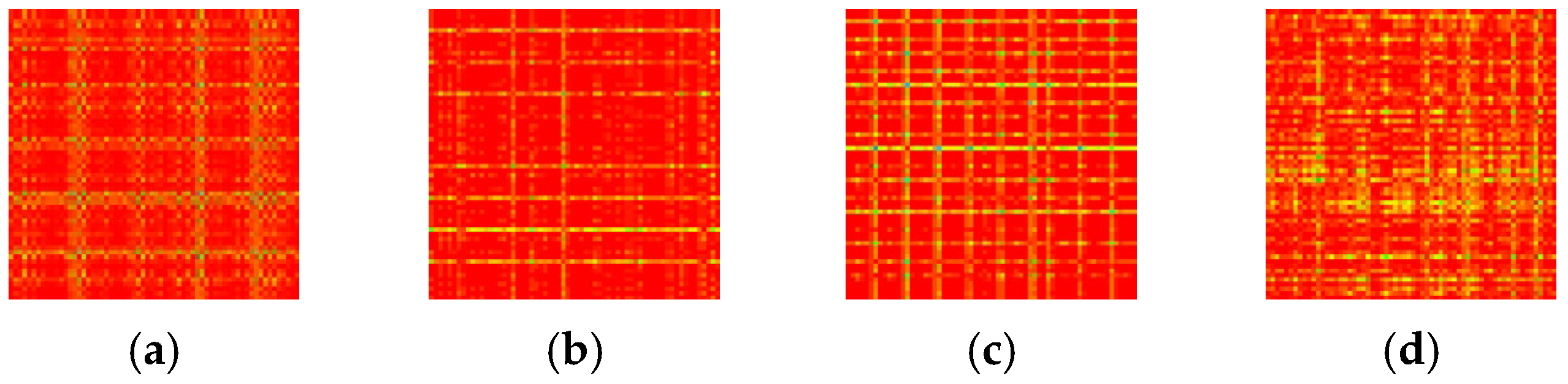
In our study, signals corresponding to the 0 hp load condition and 0.021 in fault diameter were selected. All vibration signals come from the drive end bearings. The data used includes four categories: health state (H), inner-race faul (IF), outer-race fault (OF), and ball bearing fault (BF). Each sample contains 2048 data points, with a total of 400 samples prepared for training and testing. The RP conversion diagrams of the four signals are shown in Figure 2.

4.1.2. Setting of Model Parameters

For the generator, the generative model starts from a 100-dimensional latent vector. This noise is first projected and reshaped into a compact feature representation of size 4 × 4 × 512. The subsequent synthesis process relies on four up-sampling stages realized by transposed convolutions. In the first stage, 256 filters are employed, followed by batch normalization and a ReLU nonlinearity. The following two stages use 128 and 64 filters, respectively, both operating with a stride of two to enlarge the spatial resolution; each stage is also stabilized by batch normalization and activated through ReLU. The final transposed convolution outputs a three-channel image of 64 × 64 pixels, and a Tanh activation scales the intensity values to the range [−1, 1].

For the discriminator, the adversarial counterpart receives an RGB image of 64 × 64 as input. To enhance robustness, a dropout operation with a 50% rate is applied at the beginning. Then, four hierarchical convolutional blocks progressively compress the input. Each block uses a 5 × 5 kernel with a stride of two; the number of filters grows from 64 to 128, 256, and finally 512. Starting from the second block, batch normalization is introduced to stabilize training. All convolutional layers are activated by LeakyReLU with a slope of 0.2, allowing the network to retain information from negative responses. The last convolution (kernel size four) produces a scalar output that estimates whether the sample is real or generated.

For the classification model, the classification branch also works with 64 × 64 × 3 inputs. Its architecture is organized as a dual-path design. The main path begins with a 4 × 4 convolution, followed by batch normalization, ReLU, and 3 × 3 max pooling. In parallel, a shortcut path applies a 1 × 1 convolution to preserve complementary features. The outputs of both paths are concatenated to form a richer representation. After fusion, additional convolutional layers with 16 and 32 filters are stacked, each combined with batch normalization, ReLU, and pooling. The resulting feature maps are forwarded to a 24-unit fully connected layer, flattened, and refined by an SE mechanism to capture long-range dependencies. The final stage employs a fully connected layer with four outputs, followed by a softmax operator to accomplish multi-class fault recognition.

4.1.3. Fault Diagnosis Under Limited Data Conditions

A.

Network Performance with Mixed Test Set

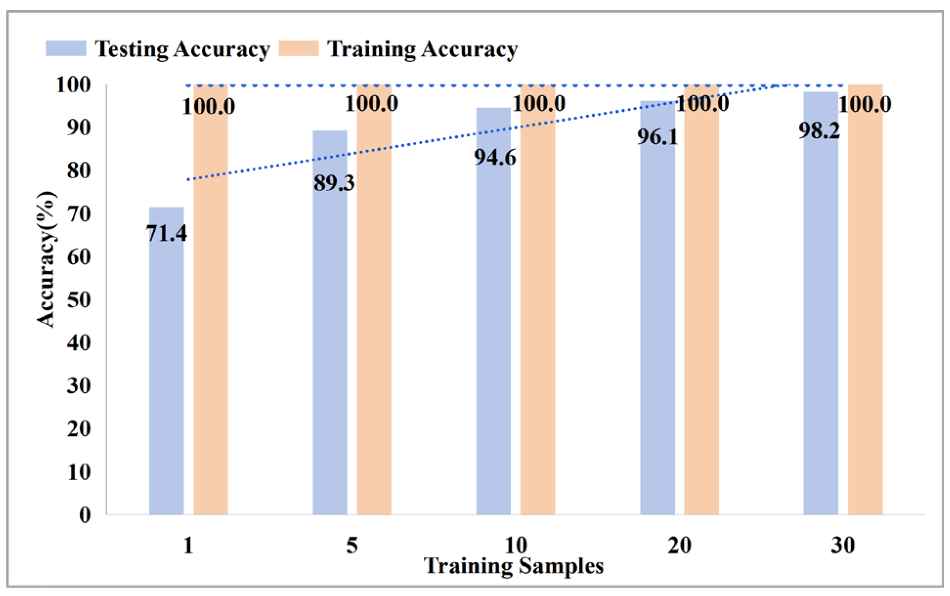
To systematically evaluate the effect of training sample size on diagnostic performance, we fixed the number of generated samples at 15 per class and gradually increased the number of real training samples to 1, 5, 10, 20, and 30. Real samples and generated samples are mixed to form the dataset, where 15 generated samples were generated by training on 30 real samples, which did not overlap with the real samples participating in the experiment. The test set and the training set are divided according to the ratio of 3:7. The experimental results are shown in Figure 3. As observed, when only one training sample per class was used, the diagnostic accuracy was limited to 71.4%. However, as the training sample size increased to 30 per class, the accuracy significantly improved to 98.2%. This finding indicates that a larger number of training samples enables the generative model to capture richer temporal dynamics, thereby improving the fidelity of synthesized data. Moreover, the enhanced diversity and representativeness of the training data contribute to a stronger generalization capability of the classification model, leading to superior diagnostic performance. Hence, the quantity of training samples plays a pivotal role in deep learning-based fault diagnosis tasks.

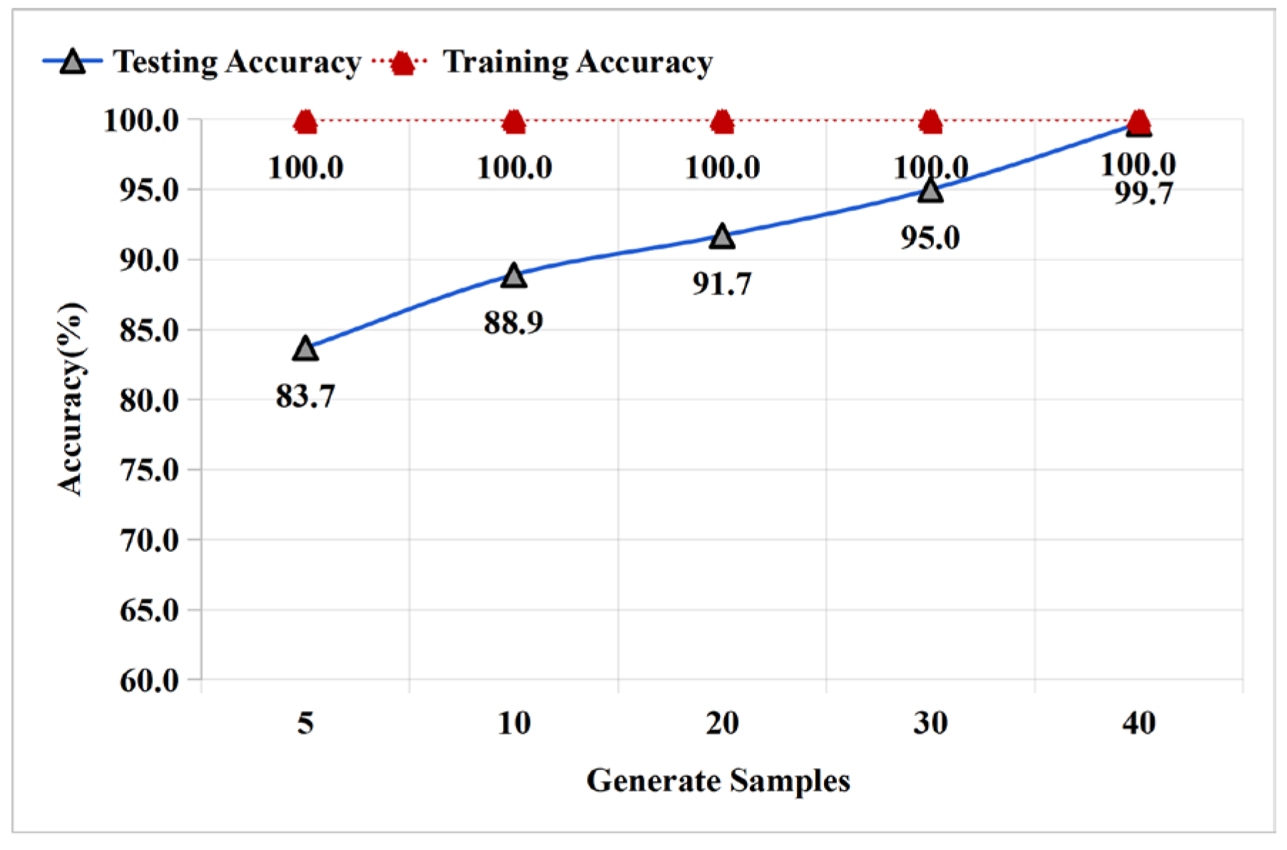
In a complementary set of experiments, we fixed the number of real training samples at 30 per class and progressively increased the number of generated samples to 5, 10, 20, 30, and 40. The dataset is equally divided into a test set and a training set in a 3:7 ratio. The results are presented in Figure 4. With only five generated samples per class, the diagnostic accuracy reached 83.7%. When the number of generated samples increased to 10, accuracy rose to 88.9%. A further increase to 20 and 30 generated samples yielded accuracies of 93.3% and 95.0%, respectively. Finally, with 40 generated samples per class, the model achieved nearly 100% accuracy. This clear upward trend highlights the significant role of data generation in enhancing classification performance under small-sample conditions. Furthermore, the introduction of the spectrum-aware module for sample screening ensured both distributional consistency and discriminability of the generated data, thereby contributing to improved diagnostic outcomes. Overall, the findings demonstrate a strong positive correlation between the number of generated samples and model accuracy, underscoring the potential of high-quality data generation to address the limitations imposed by limited training samples.

In summary, the two sets of experiments collectively demonstrate that both training sample size and generated sample size have substantial impacts on model performance. While increasing the number of training samples enhances the learning capacity of both the generative and classification models, augmenting the dataset with additional generated samples further alleviates the limitations of small sample scenarios. The synergy of these two factors effectively boosts diagnostic accuracy and robustness, providing a promising strategy for intelligent fault diagnosis under limited data conditions.

B.

Network Performance with Pure Real Test Set

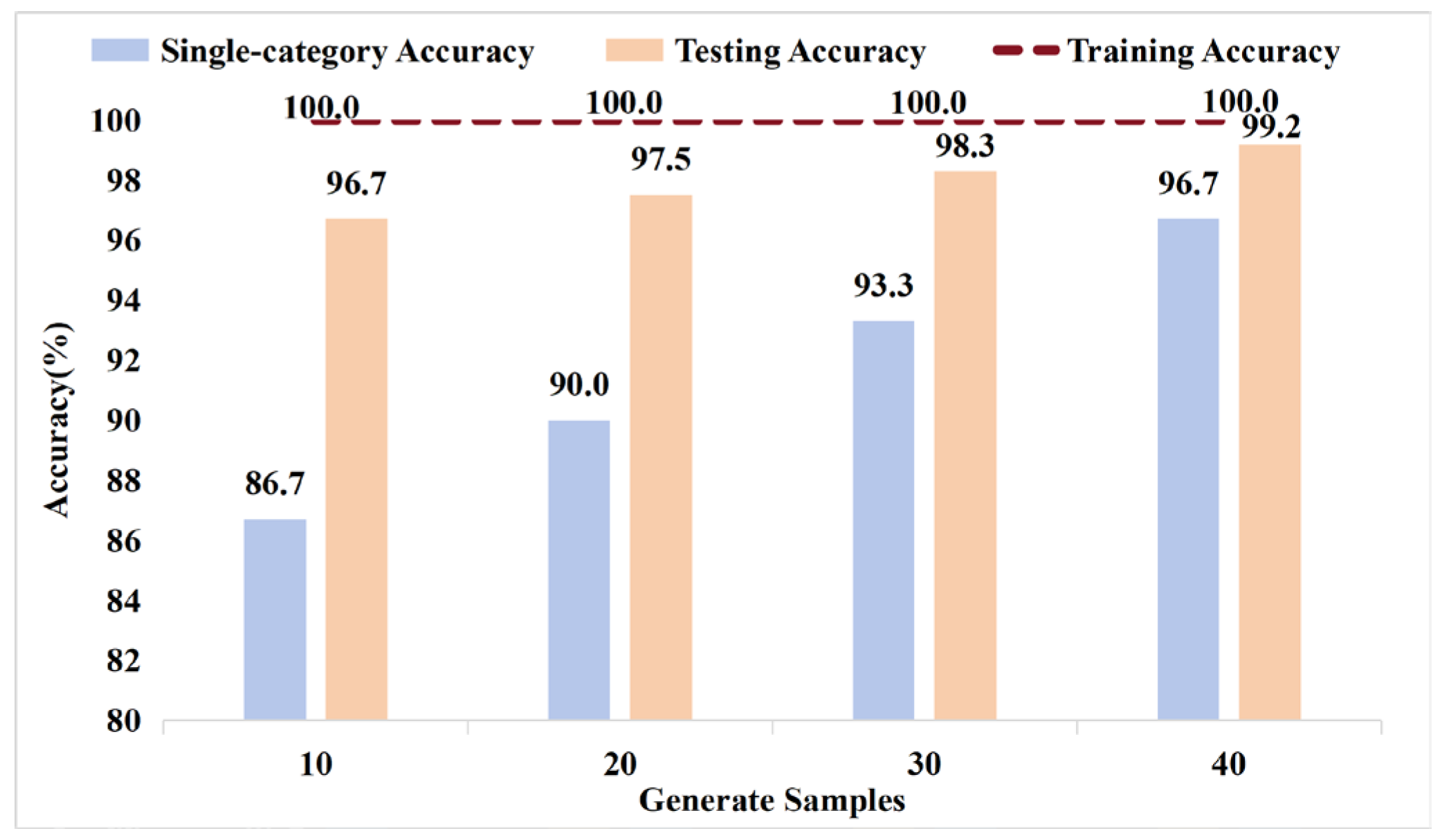
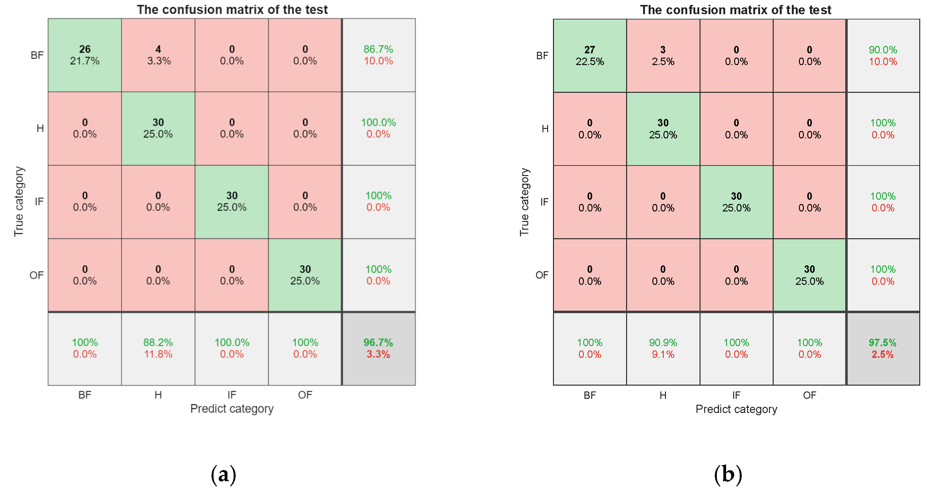
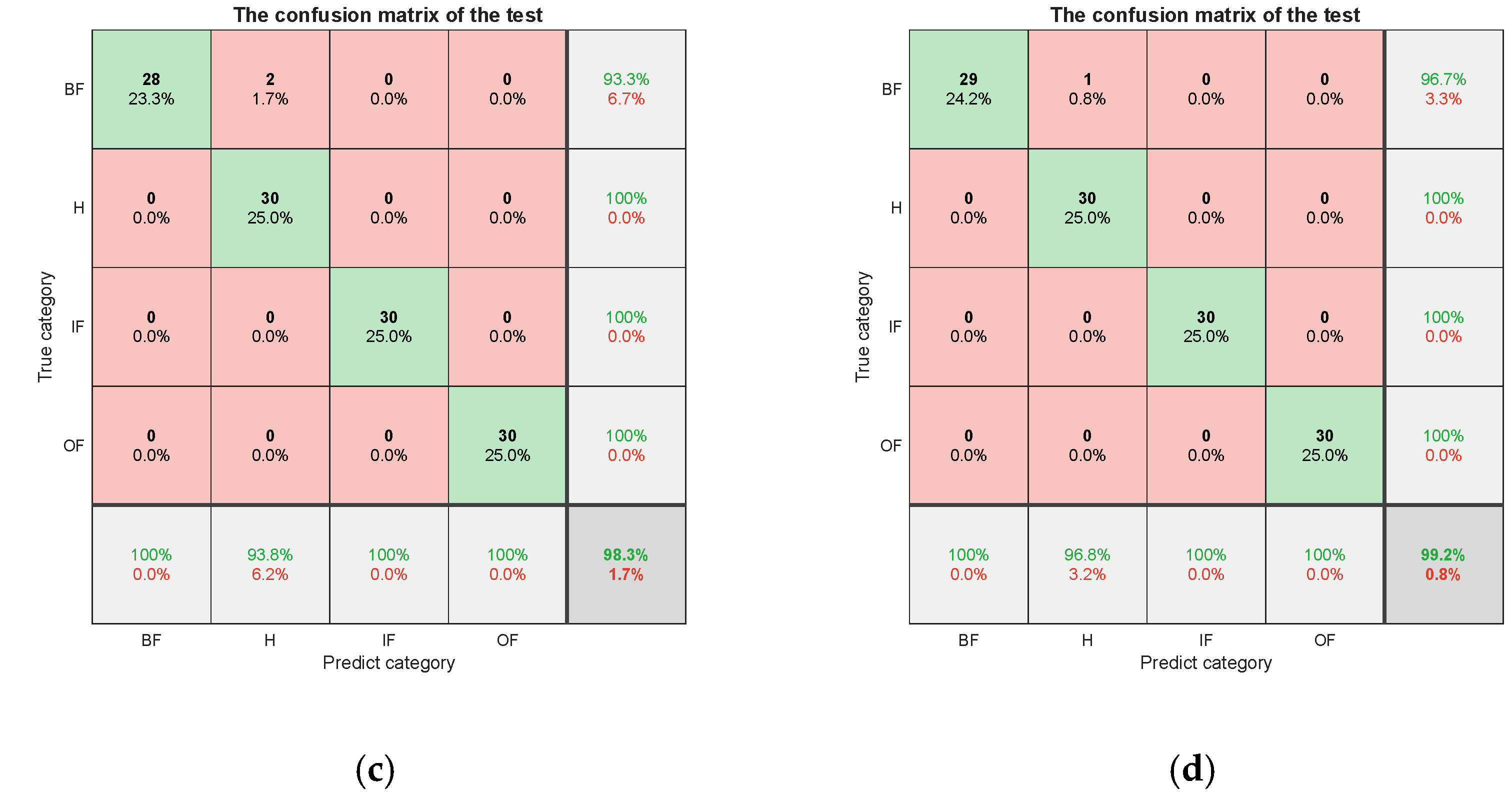
In the preceding experiments, we evaluated the impact of training and generated sample sizes. However, since both the training and testing sets were constructed by randomly mixing real and generated samples to verify the superiority of ResNet-SE, we adopted the following protocol: Five real samples were selected for the training set to generate 50 synthetic samples. Subsequently, 30 samples were randomly selected from the remaining real data for testing. The experimental results are illustrated in Figure 5 and Figure 6.

As the number of generated samples increased from 10 to 40, the single-class recognition accuracy rose from 86.7% to 100%, and the overall model accuracy improved from 96.7% to 99.2%. These results further validate the effectiveness of the proposed method.

4.1.4. Comparison with State-of-the-Art Methods

To further evaluate the effectiveness of the proposed method, we used diagnostic accuracy as a benchmark and compared it with several recently published generative adversarial-based diagnostic models. The baseline approaches considered in this study include the E-GAN, the GAN-based imbalanced diagnosis method (ACWGAN-GP) [37], the few-shot GAN [38], and the Conditional Variational Autoencoder (CVAE) [39]. The corresponding results are summarized in the comparative

Table 1. Comparison of diagnostic accuracy with state-of-the-art methods.

Method	Training Samples	Generated Samples	Accuracy (%)
E-GAN	100	50	96.0
ACWGAN-GP	150	100	94.5
Few-Shot GAN	50	50	95.2
CVAE	20	100	88.3
ResNet-SE (Proposed)	20	100	98.1
	30	50	99.7

.

The results show that when the training data are highly imbalanced, the accuracy of the enhanced GAN diagnostic model is about 96%, while the performance of the GAN-based imbalance diagnostic model remains about 94.5%. The few-shot GAN demonstrates clear benefits in small sample environments, reaching 95.2% accuracy with only 50 authentic samples combined with 50 generated ones. The CVAE, when trained with 20 real samples and supplemented with 100 generated samples, achieves an accuracy of 88.3%, highlighting both its potential and its current limitations relative to GAN-based solutions. In contrast, our proposed method requires merely 20 real samples together with 100 generated samples to obtain a 98.1% accuracy. By using 30 real samples together with 50 generated samples, the diagnostic accuracy reaches 99.7%, surpassing the majority of existing approaches in scenarios with limited data. These findings confirm that our framework leverages both global and spectral properties of vibration signals to generate high-fidelity synthetic data. Furthermore, by embedding residual learning and multi-scale attention within the classifier, it significantly enhances diagnostic robustness even under highly constrained data conditions.

4.1.5. Comparative Analysis with Different Classifiers

To further highlight the advantages of the proposed ResNet-SE model, we conducted comparative experiments against conventional CNNs, ResNet, and GAN-augmented CNN classifiers. The results are summarized in

Table 2. Comparison of classifier performance with different methods.

Method	Training Samples	Generated Samples	Accuracy (%)
CNN	30	0	93.5
ResNet	30	0	96.8
GAN-generated + CNN	30	50	97.6
ResNet-SE (Proposed)	30	0	97.9
	30	50	99.7

. With 30 training samples, the baseline CNN achieved an accuracy of only 93.5%, as it struggled to capture cross-scale features effectively. ResNet, benefiting from residual connections, achieved an accuracy of 96.8%. When combined with GAN-generated data for augmentation, CNN performance increased to 97.6%, demonstrating the role of synthetic samples in alleviating small sample limitations. Nevertheless, our ResNet-SE model further boosted accuracy to 99.7% under the same number of authentic fault samples and generated samples. This improvement stems from the multi-scale attention mechanism, which jointly models local details and global patterns, complementing the residual structure. As a result, the classifier achieves a significantly stronger generalization capability, even under restricted data availability.

4.2. Stator Interturn Fault Dataset

4.2.1. Dataset Introduction

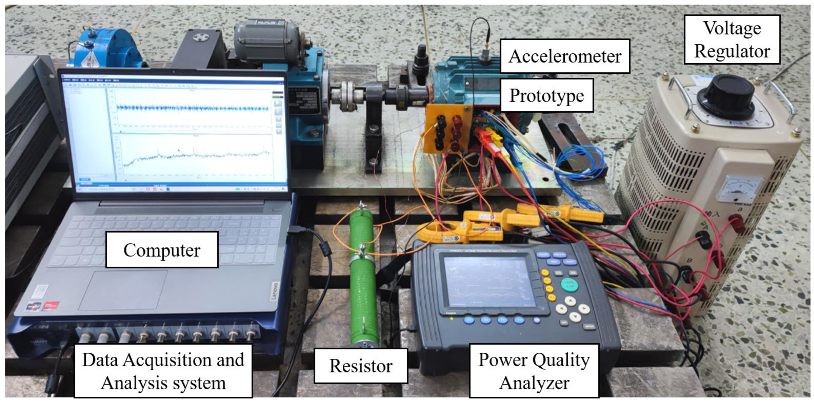
The above experimental verification and result analysis are carried out based on the general data set, which not only confirms that the proposed method has good effectiveness and generalization ability, but also finds that the method still needs to be extended to more fault-type diagnostic scenarios. To this end, this paper builds a data acquisition platform for the motor inter-turn short circuit fault, as shown in Figure 7. The YE2-80M2-2 cage induction motor, supplied by Shanghai Libiao Electric Machine Co., Ltd. (Shanghai, China), is used in the experiment, and the sampling frequency is 16.384 kHz. And its main performance parameters are shown in

Table 3. Main parameters of the experimental motor.

Parameters	Value	Parameters	Value
Rated power/kW	3	Rated current/A	5.2
Rated frequency/Hz	37.5	Core length/mm	70
Phase resistance/Ω	3.4	Motor pole number	6
Outer diameter of stator core/mm	210	Inner diameter of stator core/mm	148
Winding connection mode	Y	Number of parallel branches	1

. The experimental condition is set to no-load operation, and the detailed setting of the degree of short circuit fault between different turns of the motor is shown in

Table 4. Motor fault degree.

Fault Condition Diagnostic Classification	a	b	c	d	e	f
Number of faulty turns	0	5	15	25	35	45
η/%	0	1.96	5.86	9.76	13.67	17.58

.

In this study, the sampling conditions were set clearly. A single sample contained 1024 data points, and a total of 480 samples were prepared for model training and testing. The recurrence plot (RP) method is used to transform the signal, and the visualization results of the recurrence plot corresponding to the six signals are shown in Figure 8.

4.2.2. Fault Diagnosis Under Limited Data Conditions

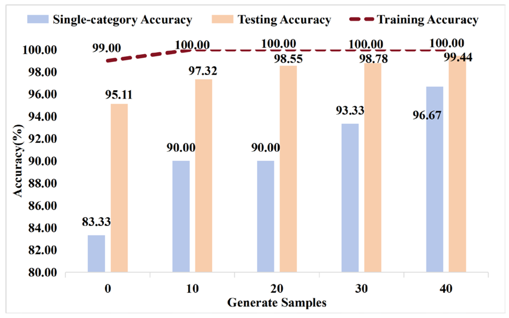
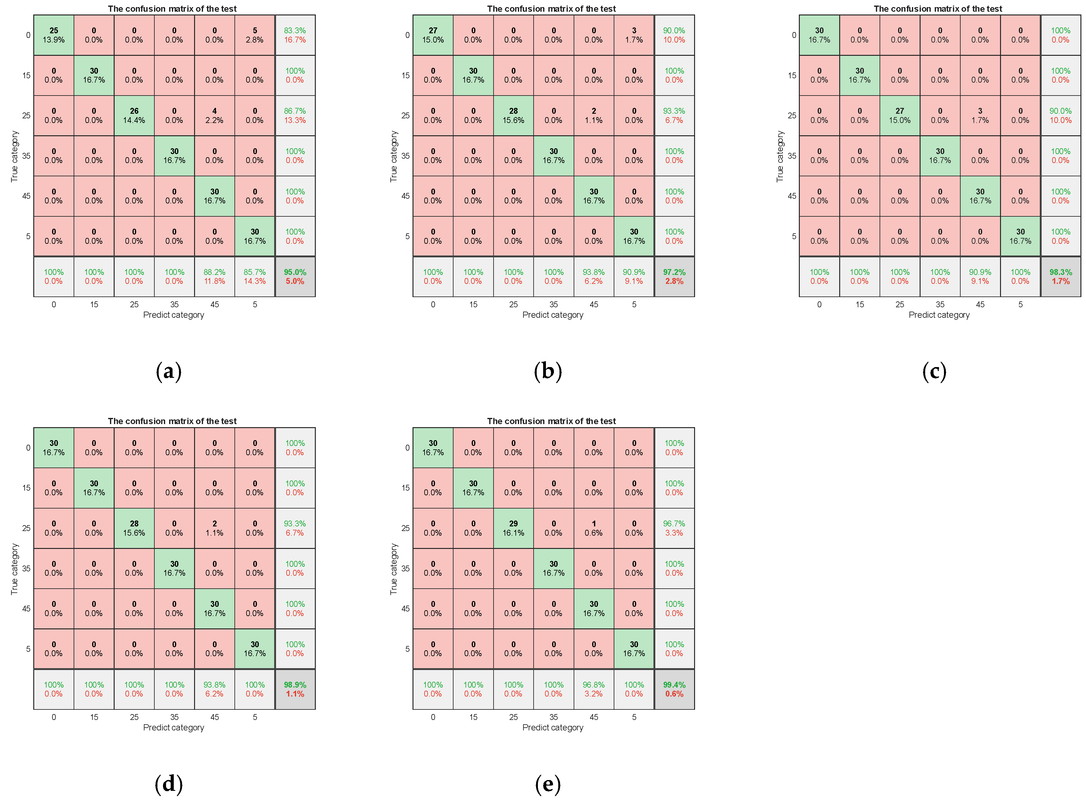
In this experiment, 10 real samples were selected as the training set, and 50 synthetic samples were generated based on the training set. Subsequently, 50 samples were randomly selected from the remaining real samples as the test set. The experimental results are shown in Figure 9. In order to ensure the reliability and rigor of the experiment, all the training and test results in this study used the mean value of repeated experiments. Figure 10 shows the confusion matrix, which is closest to the average accuracy in the training process. When the number of generated samples increases from 0 to 40, the accuracy of single-class fault recognition increases from 83.33% to 96.67%, and the overall recognition accuracy of the model also increases from 95.11% to 99.44%. The above experimental results fully verify the effectiveness and feasibility of the proposed method in the fault diagnosis of motor inter-turn short circuit.

According to the confusion matrix analysis, the classification confusion only occurs between the healthy condition and the 5-turn short circuit, 25-turn short circuit, and 45-turn short circuit categories. The experimental results show that the fault diagnosis performance of the model is significantly improved after the introduction of the generated samples. This shows that the generated samples can effectively make up for the limitation of the insufficient number of samples in the original data set. At the same time, the accuracy of the fault diagnosis continues to rise with the increase in the expanded samples, which also confirms that the diagnostic model is prone to under-fitting problems under the condition of small samples, and further verifies the rationality and effectiveness of the sample expansion strategy proposed in this paper.

4.3. HUST Fault Dataset

4.3.1. Dataset Introduction

The experiment of this study is based on the HUST data set constructed by the Intelligent Diagnosis and Health Monitoring Laboratory of Huazhong University of Science and Technology [40], and the data acquisition is completed based on the Spectra-Quest mechanical fault simulation experiment platform. The data set covers multiple types of motor fault samples and independent bearing test samples. In this paper, the motor fault data set is used to verify the diagnostic performance of the proposed method. At the same time, the small fault diagnosis test is carried out based on the bearing data set to further explore the generalization ability of the method.

The motor fault data acquisition system is mainly composed of a speed controller, an induction motor, a drive shaft, an accelerometer, and a data acquisition device. The data set contains six motor operating states: health state (H), bearing fault (BF), rotor bending fault (BOW), rotor broken bar fault (BRO), rotor misalignment fault (MISAL), and voltage unbalance fault (UNBAL). All fault types are implanted artificially, and all kinds of faults are tested by independent motor samples.

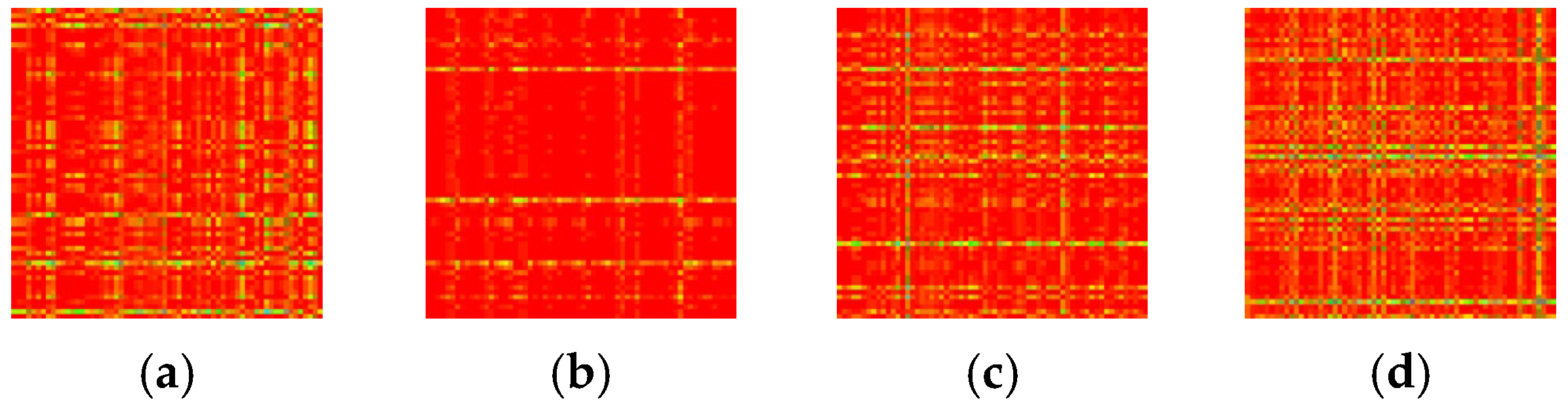
In the motor fault diagnosis experiment, the vibration signal collected under the condition of 5 Hz is selected, the sampling frequency is set to 25.6 kHz, and the length of the single sample data is 2048 sampling points. In order to fully explore the temporal correlation and internal structural characteristics of vibration signals, this paper uses the RP to convert one-dimensional time-domain vibration signals into two-dimensional grayscale images. For each operating condition, 100 RP images are generated for subsequent model training and testing. This transformation method can not only effectively improve the feature representation ability of the original data, but also lay a data foundation for the feature learning and fault classification of the deep learning model. The RP conversion results of six typical state signals are shown in Figure 11.

The bearing test system is composed of a speed controller, a motor, a shaft, an accelerometer, a bearing shell, and a data acquisition system, which can realize the controllable simulation of various bearing faults. The bearing data covers nine health states: (1) normal state; (2) moderate inner-race fault; (3) severe inner-race fault; (4) moderate outer-race fault; (5) severe outer-race fault; (6) moderate rolling element fault; (7) severe rolling element failure; (8) moderate compound fault; and (9) severe compound fault. A compound fault means that the inner ring and the outer ring have defects at the same time. All faults were manually introduced to ensure the controllability and repeatability of the experiment.

In the bearing expansion experiment, the vibration signal under the working condition of 60 Hz is selected, and four typical working conditions are focused on: health state (H), inner-race faul (IF), outer-race fault (OF), and rolling element fault (RF). The sampling frequency is set to 25.6 kHz, each acquisition lasts for 1 s, and each sample contains 2048 data points. After the RP method, the RP conversion diagram of the four signals is shown in Figure 12.

4.3.2. Fault Diagnosis Under Limited Data Conditions

A.

Motor fault diagnosis verification

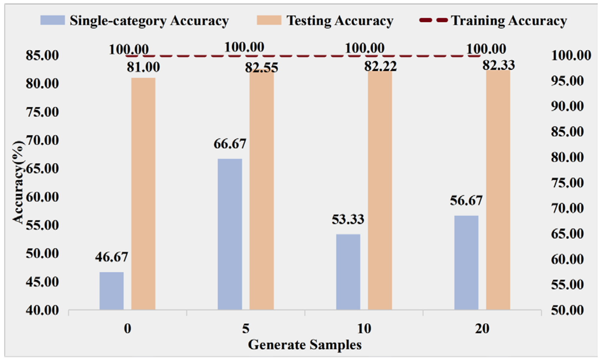
Different from the above experiments, this group of fault data covers both electrical faults and mechanical faults. A total of 80 sets of sample data were constructed in the experiment, 50 healthy samples and 30 fault samples were set, and the 30 samples that did not participate in the training were divided into the test sets. Based on 30 real fault samples, the sample generation is carried out, and the original 30 fault samples are mixed with the expanded number of 0, 5, 10, and 20 in turn to construct multiple sets of training sets with different ratios. Each group of experiments repeated training five times, and the mean value of the results was taken. The experimental statistical results are shown in Figure 13.

The experimental results show that after introducing the generated fault samples, the overall diagnostic accuracy of the model shows a significant improvement trend compared with the benchmark scheme. Although the accuracy fluctuates slightly when 10 and 20 new samples are added, the overall recognition accuracy is still significantly higher than the benchmark level without sample expansion. It is difficult to fully cover the feature distribution of various types of faults by relying only on 30 real fault training samples. The model has a slight under-fitting phenomenon and cannot fully learn the inherent characteristics of the fault, resulting in limited fault diagnosis accuracy under the benchmark conditions.

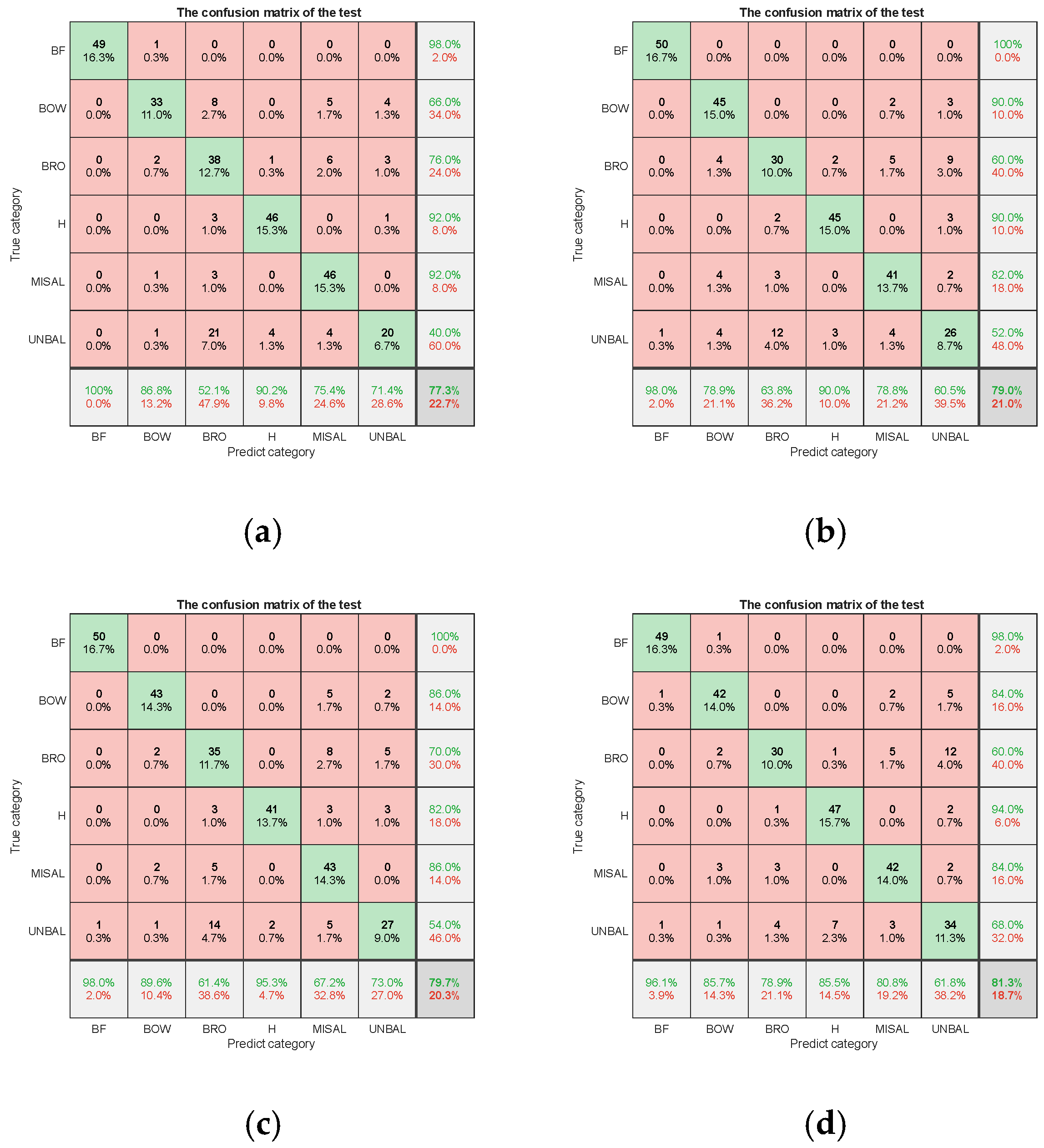
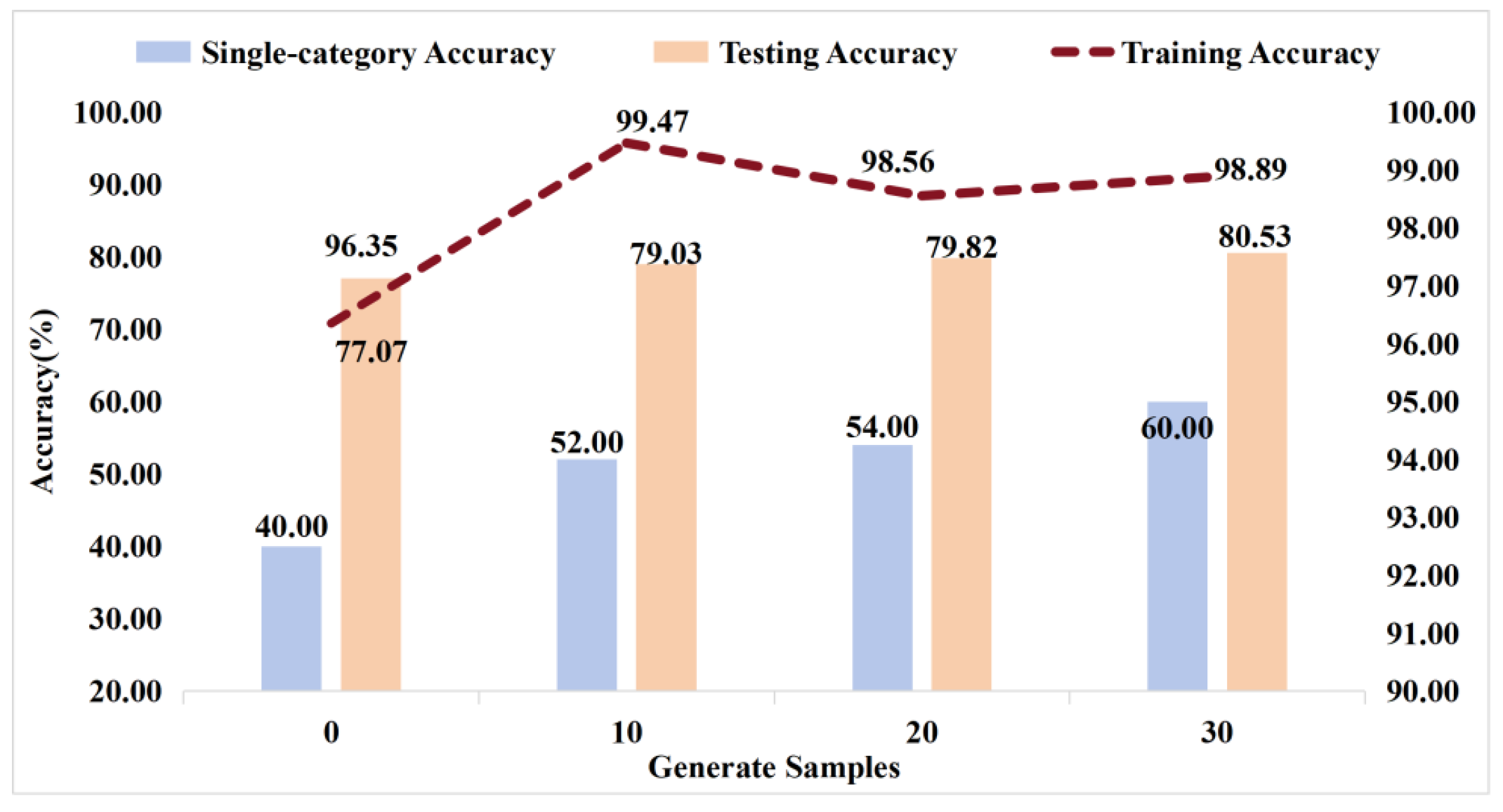
In order to further fully exploit the value of the fault data, this paper verifies the fault diagnosis performance of all the remaining real samples that have not participated in the training. The relevant results are shown in Figure 14 and Figure 15. Under the baseline condition that only 30 real training samples are set for each type and no generated samples are introduced, the diagnostic accuracy of the model is 77.07%. After adding 10 generated samples to each category, the accuracy rate is increased to 79.03%. As the number of generated samples increased to 20 and 30, the diagnostic accuracy further increased steadily to 79.82% and 80.53%, and the overall accuracy increased by 3.5%. Under the harsh conditions of the small samples in the HUST dataset, the proposed method still shows excellent diagnostic reliability and robustness, and also reflects the inherent challenges faced by fault diagnosis in a very small amount of data expansion scenarios.

By analyzing the confusion matrix in Figure 15, it can be seen that the main reason for the low diagnostic accuracy of the model is that the voltage unbalance fault (UNBAL) is easy to misclassify with other types of faults. Comparing Figure 15a,b, it can be found that after the introduction of the generated samples, the overall number of correctly classified samples increased from 232 to 244. Among them, the number of correct classifications of easily confused rotor broken bar faults (BRO) and voltage imbalance faults (UNBAL) increased from 58 to 64, and the classification effect of rotor bending faults (BOW) was also significantly improved. Further experiments were conducted without adding generated samples. Further experiments were conducted without adding generated samples. Focusing solely on identifying mechanical failures, the model can achieve a diagnostic accuracy of 93.6%, and electrical faults can reach 95.0%. This also shows that the model still has certain recognition limitations in the coexistence of electrical and mechanical multiple mixed faults.

B.

Bearing fault diagnosis verification

In order to further expand and verify the generalization performance of the proposed method, an extended experiment is carried out in this paper. The previous set of experiments indicates that the diagnostic effect of the bearing fault (BF) feature recognition is high. Therefore, this part subdivides the bearing faults in detail and focuses on the fault diagnosis performance of four working conditions: health state (H), inner-race fault (IF), outer-race fault (OF), and rolling element fault (RF).

In this group of experiments, the number of healthy samples was 30, and the test set was 30 samples that had not participated in the training. On the one hand, without adding the generated samples, the fault diagnosis of 10, 20, 24, 27, and 30 is gradually realized. On the other hand, the diagnosis of adding the generated samples in proportion is checked, and the average value of five experiments is taken, and the table is drawn. As shown in

Table 5. The accuracy and standard deviation of the DCGAN-ResNet-SE model on the HUST bearing fault dataset.

Sample Distribution	Case 1	Case 2	Case 3	Case 4	Case 5	Case 6	Case 7	Case 8
Training set real samples	10	20	24	24	24	27	27	30
Training set generates samples	0	0	0	3	6	0	3	0
Accuracy (%)	87.36	94.14	95.29	96.14	96.21	96.43	97.07	97.79
Standard deviation	2.796	1.277	1.273	0.686	1.198	1.213	0.684	0.688

.

In the absence of generated samples, when the fault sample is 30, the model achieves a 97.79% fault diagnosis. The high-precision classification effect of residual network-SE is illustrated. When we add the generated samples according to 10% and 20% of the fault samples, the diagnostic accuracy of the model is improved, indicating that the DCGAN algorithm based on spectrum-aware filtering generates high-quality samples and can achieve the effect of balancing samples. At the same time, we observe that the accurate standard deviation of all the models added to the generated samples is smaller than that of the models not added to the generated samples. It indirectly shows that the stability of model training is also improved after data enhancement by the DCGAN algorithm based on the spectrum-aware filtering method.

In order to verify the effectiveness of the data expansion of the generative network in the small sample fault diagnosis scenario, this paper designs multiple sets of control experiments. By adjusting the ratio of the number of healthy samples and fault samples in the training set, and setting different generation sample introduction strategies, the influence of the generated samples on the diagnostic performance and training stability of the model is systematically analyzed.

When only a single mechanical fault or a single electrical fault is identified, various types of faults have a more significant feature distribution. The gradual introduction of generated samples can effectively expand the diversity of fault features and significantly alleviate the modeling limitations caused by the scarcity of small sample data. In the complex scene with cross-condition and multi-fault types in the training set, even if the number of generated samples continues to increase, the improvement of classification accuracy gradually slows down, and it is difficult to achieve a significant increase due to factors such as the saturation of the model learning capacity and the limited inherent discriminant characteristics of the original data.

By comparing the accuracy and standard deviation of multiple rounds of repeated experiments, it can be found that the standard deviation of the training results after the introduction of the generated samples is lower. This shows that the generated samples not only improve the classification accuracy of the model in the adaptation scenario, but also effectively enhance the training stability and generalization robustness of the model. There are differences in the improvement of model performance on different data sets, which are mainly determined by the separability of sample categories, data complexity, and fault feature richness. This result further confirms that the proposed generation network expansion method has good adaptability and versatility, and can provide reliable technical support for equipment fault diagnosis under small sample conditions.

5. Conclusions

To address the challenge of insufficient training samples in motor fault diagnosis, this work proposes a DCGAN-based method with a spectrum-aware screening mechanism. Taking vibration signals as the research object, by integrating image constraints with high spectral similarity into the generative network, the proposed approach improves both the distributional consistency and the discriminative power of synthetic samples, thereby ensuring higher quality signal generation. For classification, a ResNet enhanced with an SE module is designed to capture both local details and global temporal dependencies, leading to more robust feature representations. Extensive experiments were conducted on the CWRU fault datasets, the stator interturn fault dataset, and the HUST fault datasets. The results demonstrate the effectiveness of the method under limited data conditions. For example, on the HUST motor fault dataset, the diagnostic accuracy increased by 2% after adding the generated samples. For the stator inter-turn short circuit fault dataset, the diagnostic accuracy 95.11% without generating samples, and increased to 99.44% when 40 generated samples per class were used. On the CWRU dataset, the model achieved nearly 100% accuracy, confirming the strong generalization capability of the approach. Moreover, the key novelty of this work lies in the spectrum-aware closed-loop design, which distinguishes our approach from conventional loss-regularized GANs. By screening and rejecting frequency-consistent samples, we ensure both stability and diversity in small sample augmentation. In addition, the integration of a ResNet-SE classifier allows for the simultaneous capture of local and global features, achieving superior accuracy under highly constrained conditions. This dual-level innovation, at both the data generation and classification stages, provides a systematic solution to small sample motor fault diagnosis, with a strong potential for extension to other rotating machinery.

The future research directions will focus on addressing the limitations of laboratory-based data and further enhancing the practicality and adaptability of the proposed method. On the one hand, we will study fault diagnosis methods under variable operating conditions and strong noise environments, aiming to narrow the gap between laboratory research and real-world applications. On the other hand, we will optimize the generative network to adapt to different types of motor faults and motor models (e.g., high-voltage industrial motors and permanent magnet synchronous motors), improving the generalization ability of synthetic samples across diverse fault categories and motor configurations. Finally, we will investigate the combination of the spectrum-aware GAN frameworks with transfer learning or federated learning to address the problem of insufficient labeled real-world fault data, further improving the diagnostic performance and practical value of the method in small-sample industrial scenarios.

References

1. Shan, H.; Zhang, X.; Liang, W.; Wu, Z.; Shao, H.; Qin, G. A Prototype Learning Framework Based on Continual Learning for Motor Incremental Fault Diagnosis Under Few-Shot Conditions. IEEE Trans. Instrum. Meas. 2025, 74, 3556211. [Google Scholar] [CrossRef]
2. Chen, H.T.; Jiang, B.; Ding, S.X.; Huang, B. Data-driven fault diagnosis for traction systems in high-speed trains: A survey, challenges, and perspectives. IEEE Trans. Intell. Transp. Syst. 2022, 23, 1700–1716. [Google Scholar] [CrossRef]
3. Aslan, B.; Balci, S.; Kayabasi, A. Fault diagnosis in thermal images of transformer and asynchronous motor through semantic segmentation and different CNN models. Appl. Therm. Eng. 2025, 265, 125599. [Google Scholar] [CrossRef]
4. Chen, Z.W.; Liang, K.T.; Ding, S.X.; Yang, C.; Peng, T.; Yuan, X.F. A comparative study of deep neural network-aided canonical correlation analysis-based process monitoring and fault detection methods. IEEE Trans. Neural Netw. Learn. Syst. 2022, 33, 6158–6172. [Google Scholar] [CrossRef] [PubMed]
5. Aguiar, G.; Krawczyk, B.; Cano, A. A survey on learning from imbalanced data streams: Taxonomy, challenges, empirical study, and reproducible experimental framework. Mach. Learn. 2024, 113, 4165–4243. [Google Scholar] [CrossRef]
6. Mohammad-Alikhani, A.; Jamshidpour, E.; Dhale, S.; Akrami, M.; Pardhan, S.; Nahid-Mobarakeh, B. Fault Diagnosis of Electric Motors by a Channel-Wise Regulated CNN and Differential of STFT. IEEE Trans. Ind. Appl. 2025, 61, 3066–3077. [Google Scholar] [CrossRef]
7. Chen, H.T.; Luo, H.; Huang, B.; Jiang, B.; Kaynak, O. Transfer learning-motivated intelligent fault diagnosis designs: A survey, insights, and perspectives. IEEE Trans. Neural Netw. Learn. Syst. 2024, 35, 2969–2983. [Google Scholar] [CrossRef]
8. Wu, Z.Y.; Lin, W.F.; Fu, B.H.; Guo, J.C.; Ji, Y.; Pecht, M. A local adaptive minority selection and oversampling method for class-imbalanced fault diagnostics in industrial systems. IEEE Trans. Reliab. 2020, 69, 1195–1206. [Google Scholar] [CrossRef]
9. Shih, K.; Ngo, D.; Huang, S.; Hsieh, M.-F. Mixed-Fault Diagnosis for Permanent Magnet Motor with Few-Shot Learning Based on the Prototypical Network. IET Electr. Power Appl. 2025, 19, e70081. [Google Scholar] [CrossRef]
10. Han, S.; Cheng, L. A multi-stage framework for motor vibration fault diagnosis based on long-term time series forecasting and deep feature classification. Control Eng. Pract. 2026, 168, 106685. [Google Scholar] [CrossRef]
11. Xia, P.; Huang, Y.; Liu, C.; Liu, J. Learn to Supervise: Deep Reinforcement Learning-Based Prototype Refinement for Few-Shot Motor Fault Diagnosis. IEEE Trans. Neural Netw. Learn. Syst. 2025, 36, 11428–11442. [Google Scholar] [CrossRef] [PubMed]
12. Chen, G.; Li, S.; He, Q.; Zhou, P.; Zhang, Q.; Yang, G.; Lv, D. Fault diagnosis of drone motors driven by current signal data with few samples. Meas. Sci. Technol. 2024, 35, 086202. [Google Scholar] [CrossRef]
13. Aggarwal, A.; Mittal, M.; Battineni, G. Generative adversarial network: An overview of theory and applications. Int. J. Inf. Manag. Data Insights 2021, 1, 100004. [Google Scholar] [CrossRef]
14. Xu, Z.F.; Liu, D.; Zhang, Y.F.; Wang, M.; Huang, Q.; Wang, X. Fault diagnosis of rolling bearings based on block 2D principal component analysis and depth separable convolution model. J. Mech. Sci. Technol. 2025, 39, 4277–4291. [Google Scholar] [CrossRef]
15. Zhao, Y.J.; Zhou, M.L.; Xu, X.Z.; Zhang, N.N. Fault diagnosis of rolling bearings with noise signal based on modified kernel principal component analysis and DC-ResNet. CAAI Trans. Intell. Technol. 2023, 8, 1014–1028. [Google Scholar] [CrossRef]
16. Zhang, G.Q.; Wang, B.; Li, J.; Xu, Y.L. The application of deep learning in bridge health monitoring: A literature review. Adv. Bridge Eng. 2022, 3, 22. [Google Scholar] [CrossRef]
17. Liu, Y.C.; Gao, Y.S.; Niu, R.; Zhang, Z.Y.; Lu, G.W.; Hu, H.F.; Liu, T.G.; Cheng, Z.Z. Rapid and accurate bacteria identification through deep-learning-based two-dimensional Raman spectroscopy. Anal. Chim. Acta 2024, 1332, 343376. [Google Scholar] [CrossRef]
18. Nguyen, T.D.; Nguyen, H.C.; Pham, D.H.; Nguyen, P.D. A distinguished deep learning method for gear fault classification using time-frequency representation. Discov. Appl. Sci. 2024, 6, 340. [Google Scholar] [CrossRef]
19. Wang, R.G.; Zhang, S.H.; Chen, Z.Y.; Li, W.H. Enhanced generative adversarial network for extremely imbalanced fault diagnosis of rotating machine. Measurement 2021, 180, 109467. [Google Scholar] [CrossRef]
20. Li, H.Z.; Yao, L.N. Motor Fault Diagnosis Based on Generative Adversarial Network Using Hyperchaotic Sequences and Mixed-Dimensional Network. IEEE Trans. Ind. Inform. 2025, 21, 3216–3225. [Google Scholar] [CrossRef]
21. Vo, T.T.; Liu, M.K. Residual signal-driven GAN framework for robust induction motor fault diagnosis under data scarcity conditions. Expert Syst. Appl. 2026, 301, 130513. [Google Scholar] [CrossRef]
22. Zhang, D.; Ning, Z.Q.; Yang, B.; Wang, T.Y.; Ma, Y.J. Fault diagnosis of permanent magnet motor based on DCGAN-RCCNN. Energy Rep. 2022, 8, 616–626. [Google Scholar] [CrossRef]
23. Gao, W.; Jin, H.; Yang, G.J. Series arc fault diagnosis method of photovoltaic arrays based on GASF and improved DCGAN. Adv. Eng. Inform. 2022, 54, 101809. [Google Scholar] [CrossRef]
24. Chen, L.M.; Jin, L.; Shang, M.S. Efficient loss landscape reshaping for convolutional neural networks. IEEE Trans. Neural Netw. Learn. Syst. 2025, 36, 12535–12549. [Google Scholar] [CrossRef] [PubMed]
25. Wen, L.; Li, X.Y.; Gao, L.; Zhang, Y.Y. A new convolutional neural network-based data-driven fault diagnosis method. IEEE Trans. Ind. Electron. 2018, 65, 5990–5998. [Google Scholar] [CrossRef]
26. Cheng, Y.; Gu, H.; Song, D.; Ma, L.; Tao, L. Fault diagnosis for driving motor with insufficient fault data: A data transfer generation method. Int. J. Adv. Manuf. Technol. 2024, 134, 1195–1218. [Google Scholar] [CrossRef]
27. Fu, Z.; Liu, Z.; Ping, S.; Li, W.; Liu, J. TRA-ACGAN: A Motor Bearing Fault Diagnosis Model Based on an Auxiliary Classifier Generative Adversarial Network and Transformer Network. ISA Trans. 2024, 149, 381–393. [Google Scholar] [CrossRef]
28. Xie, F.Y.; Li, G.; Hu, W.; Fan, Q.Y.; Zhou, S.T. Intelligent fault diagnosis of variable-condition motors using a dual-mode fusion attention residual. J. Mar. Sci. Eng. 2023, 11, 1385. [Google Scholar] [CrossRef]
29. Pandiyan, M.; Babu, T.N. Systematic review on fault diagnosis on rolling-element bearing. J. Vib. Eng. Technol. 2024, 12, 8249–8283. [Google Scholar] [CrossRef]
30. Wang, Q.; Huang, R.; Xiong, J.; Yang, J.; Dong, X.; Wu, Y.; Wu, Y.; Lu, T. A Survey on Fault Diagnosis of Rotating Machinery Based on Machine Learning. Meas. Sci. Technol. 2024, 35, 102001. [Google Scholar] [CrossRef]
31. Zhou, Y.K.; Wang, Z.Y.; Zuo, X.; Zhao, H. Identification of wear mechanisms of main bearings of marine diesel engine using recurrence plot based on CNN model. Wear 2023, 520, 204656. [Google Scholar] [CrossRef]
32. Lim, W.; Yong, K.S.C.; Lau, B.T.; Tan, C.C.L. Future of generative adversarial networks for anomaly detection in network security: A review. Comput. Secur. 2024, 139, 103733. [Google Scholar] [CrossRef]
33. Radford, A.; Metz, L.; Chintala, S. Unsupervised representation learning with deep convolutional generative adversarial networks. arXiv 2016, arXiv:1511.06434. [Google Scholar] [CrossRef]
34. He, K.M.; Zhang, X.Y.; Ren, S.Q.; Sun, J. Deep residual learning for image recognition. In Proceedings of the IEEE Conference on Computer Vision and Pattern Recognition; IEEE: New York, NY, USA, 2016; pp. 770–778. [Google Scholar]
35. Yang, Y.; Jing, J.; Zhang, J.; Liu, Z.; Li, X. Discriminative fault diagnosis transfer learning network under joint mechanism. Sci. Rep. 2025, 15, 8888. [Google Scholar] [CrossRef]
36. Yang, Y.C.; Han, C.S.; Ran, G.T.; Ma, T.Y.; Pan, J.T. Fault diagnosis of rolling element bearing based on BiTCN-attention and OCSSA mechanism. Actuators 2025, 14, 218. [Google Scholar] [CrossRef]
37. Li, Z.X.; Zheng, T.S.; Wang, Y.; Cao, Z.; Guo, Z.Q.; Fu, H.Y. A novel method for imbalanced fault diagnosis of rotating machinery based on generative adversarial networks. IEEE Trans. Instrum. Meas. 2021, 70, 3500417. [Google Scholar] [CrossRef]
38. Ren, Z.J.; Zhu, Y.S.; Liu, Z.; Feng, K. Few-shot GAN: Improving the performance of intelligent fault diagnosis in severe data imbalance. IEEE Trans. Instrum. Meas. 2023, 72, 3516814. [Google Scholar] [CrossRef]
39. Dixit, S.; Verma, N.K. Intelligent condition-based monitoring of rotary machines with few samples. IEEE Sens. J. 2020, 20, 14337–14346. [Google Scholar] [CrossRef]
40. Zhao, C.; Shen, W.; Zio, E.; Ma, H. Multimodal Unified Generalization and Translation Network for Intelligent Fault Diagnosis under Dynamic Environments. Eng. Appl. Artif. Intell. 2025, 162, 112559. [Google Scholar] [CrossRef]
Figure 1. Structure diagram of the classification model based on ResNet-SE.
Actuators 15 00299 g001
Figure 2. The RP conversion diagrams: (a) H; (b) IF; (c) OF; (d) BF.
Actuators 15 00299 g002
Figure 3. Effect of training sample size on diagnostic accuracy.
Actuators 15 00299 g003
Figure 4. Effect of generated sample size on diagnostic accuracy.
Actuators 15 00299 g004
Figure 5. The diagnostic accuracy of the proposed method.
Actuators 15 00299 g005
Figure 6. Confusion matrix: (a) 10 generated samples; (b) 20 generated samples; (c) 30 generated samples; (d) 40 generated samples.
Actuators 15 00299 g006aActuators 15 00299 g006b
Figure 7. Experimental platform of stator interturn fault.
Actuators 15 00299 g007
Figure 8. The RP conversion diagrams: (a) 0; (b) 5; (c) 15; (d) 25; (e) 35; (f) 45.
Actuators 15 00299 g008
Figure 9. The diagnostic accuracy of the proposed method.
Actuators 15 00299 g009
Figure 10. Confusion matrix: (a) 0 generated samples; (b) 10 generated samples; (c) 20 generated samples; (d) 30 generated samples; (e) 40 generated samples.
Actuators 15 00299 g010
Figure 11. The RP conversion diagrams: (a) H; (b) BF; (c) BOW; (d) BRO; (e) MISAL; (f) UNBAL.
Actuators 15 00299 g011
Figure 12. RP conversion diagram: (a) H; (b) IF; (c) OF; (d) RF.
Actuators 15 00299 g012
Figure 13. The diagnostic accuracy of the proposed method.
Actuators 15 00299 g013
Figure 14. The diagnostic accuracy of the proposed method.
Actuators 15 00299 g014
Figure 15. Confusion matrix: (a) 0 generated samples; (b) 10 generated samples; (c) 20 generated samples; (d) 30 generated samples.
Actuators 15 00299 g015