A Model-Based Backstepping Pressure Control Strategy for a Rotary Direct-Drive Pressure Valve

Abstract

Rotary direct-drive pressure valves (RDDPVs) have attracted increasing attention in aircraft braking systems because of their compact structure, reduced weight, and improved anti-contamination capability. However, the pressure regulation of RDDPVs is challenging due to the coupled dynamics among the limited-angle torque motor, eccentric spool motion, steady-state flow force, and load pressure. Existing pressure control methods for RDDPVs are still mainly based on linear controllers such as PI/PID controllers, which do not explicitly compensate for the nonlinear characteristics of the valve. To address this problem, this paper investigates the application of a model-based backstepping control strategy to RDDPV pressure regulation. First, a nonlinear dynamic model of the RDDPV is established, and a nonlinear state-space representation is derived for controller design. Based on this model, a backstepping pressure controller is developed, in which the nonlinear model information is used for feedforward compensation. Dynamic surface control is introduced to avoid direct differentiation of the virtual control signals. Lyapunov analysis shows that the closed-loop tracking errors are uniformly ultimately bounded under bounded disturbances. Comparative simulations are conducted under different reference pressure trajectories and randomized model parameter and disturbance conditions. The simulation results indicate that the proposed controller achieves better tracking performance than the controller without detailed model compensation and the conventional PI controller under the tested operating conditions. This study provides an initial simulation-based exploration of model-based nonlinear pressure control for RDDPVs.

1. Introduction

Pressure servo valves (PSVs) are key components in electro-hydraulic control systems and have been widely used in aerospace, robotics, and precision manufacturing applications [1,2,3,4]. In safety-critical systems such as aircraft braking systems, PSVs are responsible for regulating and maintaining the braking pressure, and their dynamic performance directly affects the stability and safety of the braking process [5,6]. Excessive braking pressure may generate an oversized braking torque, leading to wheel lock-up or even tire damage, whereas insufficient pressure may fail to provide the required braking force for aircraft deceleration. Therefore, accurate and fast pressure regulation is essential for aircraft braking systems.

At present, pressure servo valves used in airborne braking systems are mainly based on flapper-nozzle structures [7,8,9]. However, such valves usually have relatively complex pilot-stage structures and require high hydraulic fluid cleanliness, since the nozzles are susceptible to contaminant clogging [10,11]. These limitations may degrade pressure regulation performance and increase potential safety risks. In addition, the multi-stage structure of conventional flapper-nozzle valves often leads to increased size and weight, which is not favorable for the lightweight and compact design requirements of modern aircraft. To overcome these limitations, the rotary direct-drive pressure valve (RDDPV) has attracted increasing attention [12]. By eliminating the traditional flapper-nozzle pilot stage, the RDDPV has a simpler structure, reduced size and weight, and improved anti-contamination capability. Nevertheless, due to the coupled motor-spool dynamics, hydraulic nonlinearities, and external braking-load effects, accurate pressure control of the RDDPV remains challenging. These characteristics motivate the development of a model-based nonlinear pressure control strategy for the RDDPV.

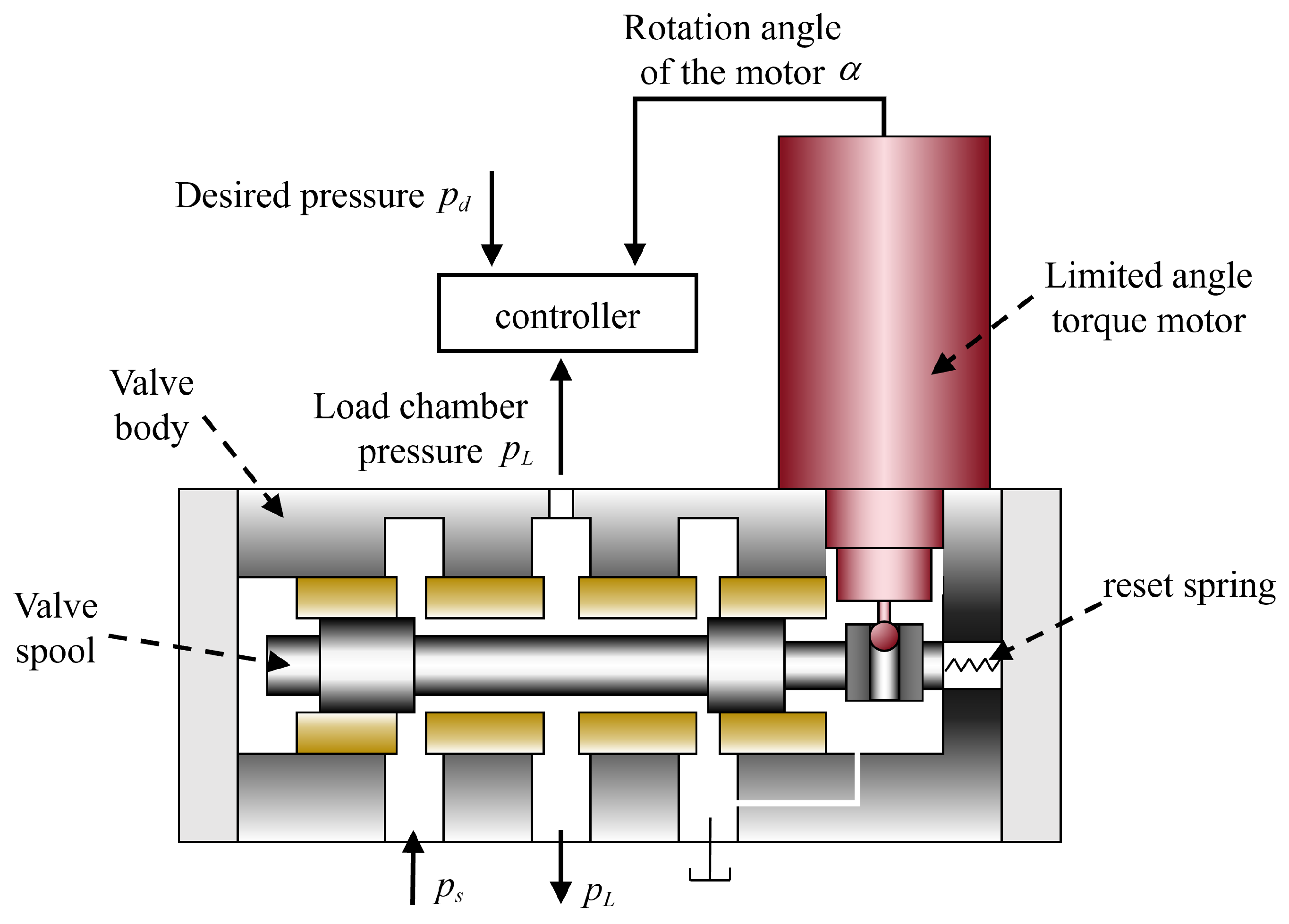
These control challenges mainly originate from the unique direct-drive structure of the RDDPV. The RDDPV is primarily composed of a limited-angle torque motor and a spool valve. The motor drives an eccentric shaft to generate the translational motion of the spool, thereby directly regulating the valve orifice opening and the load chamber pressure. Although this direct-drive structure simplifies the mechanical configuration, it also introduces strongly coupled and nonlinear system dynamics. First, the limited-angle torque motor, which acts as the driving unit, exhibits second-order dynamic characteristics due to the effects of rotational inertia and damping [13]. Second, when the eccentric shaft actuates the spool, the spool undergoes not only the desired translational motion but also a rotational motion around its axis [14]. During this process, the spool is affected by the steady-state flow force, whose magnitude varies nonlinearly with the valve orifice opening and the pressure differential, thereby influencing the spool motion [15]. Furthermore, the external braking-load characteristics are directly coupled with the pressure dynamics of the RDDPV, which further affects the pressure regulation accuracy [16]. Under the combined influence of motor dynamics, spool motion nonlinearities, hydraulic flow nonlinearities, and braking-load disturbances, conventional linear controllers may have limited ability to maintain satisfactory pressure tracking performance over a wide operating range. Therefore, it is necessary to develop a model-based nonlinear control strategy that explicitly utilizes the RDDPV dynamic model to compensate for the dominant nonlinearities and attenuate the influence of bounded disturbances.

Currently, various control methods have been investigated for pressure servo valves and related electro-hydraulic pressure regulation systems. Ref. [17] proposed a sliding mode variable-structure control strategy for a direct-drive volume-control electro-hydraulic servo system, in which pressure regulation was achieved by controlling the motor torque. In [18,19], switching valve arrays were employed in aircraft braking systems to realize braking pressure regulation and runway condition recognition. Although this type of method can avoid clogging failures associated with conventional servo valves, the coordinated operation of multiple switching valves increases the system complexity, volume, and weight, which is not favorable for the lightweight design requirements of modern aircraft braking systems. In addition, some nonlinear and robust control methods have been developed for pressure control in other fluid power systems. For example, Ref. [20] developed an extended-state-observer-based sliding mode control method for pneumatic actuator pressure control under uncertainties and disturbances, while Ref. [21] designed a model-based pressure controller for a pneumatic servo system using the backstepping method. However, due to the significant differences between pneumatic and hydraulic systems in terms of fluid compressibility, pressure level, and flow characteristics, these methods cannot be directly applied to the pressure control of RDDPVs.

Meanwhile, many advanced control methods have been reported for hydraulic servo systems, especially for position tracking control. For instance, adaptive control, disturbance observers, and observer-based control methods have been used to estimate or compensate for unknown parameters, external disturbances, and unmeasured states in hydraulic actuation systems [22,23,24]. Model-based nonlinear control methods have also been widely applied to hydraulic position servo systems to improve tracking performance under nonlinear dynamics and uncertainties [25,26,27,28,29,30,31]. Nevertheless, most of these studies focus on position control of hydraulic actuators or linear hydraulic servo systems, whereas the pressure control problem of the RDDPV involves different dynamic characteristics, including limited-angle motor dynamics, eccentric spool transmission, steady-state flow force, and load pressure dynamics. Therefore, how to establish a suitable nonlinear model and develop a model-based controller for RDDPV pressure regulation remains a problem worthy of further investigation.

Motivated by the above considerations, this paper first establishes a nonlinear dynamic model of the RDDPV, which describes the coupled relationships among the limited-angle torque motor, eccentric spool motion, steady-state flow force, and load pressure dynamics. Based on this model, a model-based backstepping pressure control strategy is developed for the RDDPV. The proposed controller uses the nonlinear model information for feedforward compensation and introduces stabilizing feedback terms to ensure that the closed-loop tracking errors are uniformly ultimately bounded under bounded disturbances. The main contributions of this paper are summarized as follows:

(1)

A nonlinear dynamic model of the RDDPV is established for pressure control design. The model describes the coupled relationships among the limited-angle torque motor dynamics, eccentric spool motion, steady-state flow force, and load pressure dynamics. Compared with studies that mainly focus on structural analysis or linearized descriptions, this model provides a nonlinear state-space representation suitable for model-based controller design.

(2)

A model-based backstepping pressure control strategy is developed for the RDDPV. Different from conventional PI/PID-based pressure regulation methods, the proposed controller explicitly uses the nonlinear model information for feedforward compensation, so that the dominant nonlinearities of the motor-spool-pressure dynamics can be considered in the control law.

(3)

Dynamic surface control is introduced into the RDDPV backstepping controller to avoid direct differentiation of the virtual control signals. The Lyapunov stability analysis proves that the closed-loop tracking errors are uniformly ultimately bounded under bounded disturbances. Comparative simulations are used to validate the proposed modeling and control framework under the considered operating conditions.

The remainder of this paper is organized as follows. Section 2 introduces the nonlinear model of the RDDPV. Section 3 details the controller design process and provides the stability proof. In Section 4, comparative simulations are conducted to evaluate the performance of the proposed controller. Finally, Section 5 concludes the paper.

2. The Nonlinear Model of RDDPV

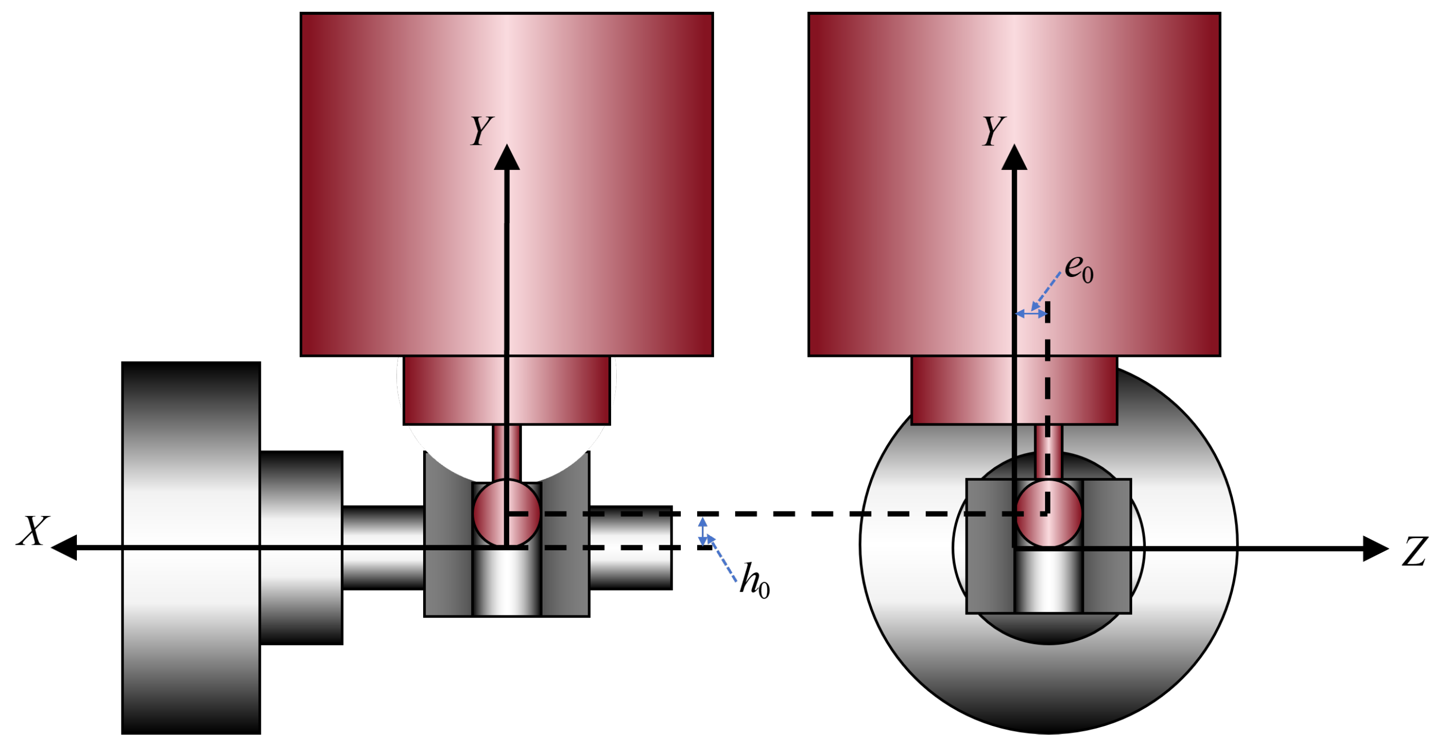
The schematic diagram of the RDDPV studied in this paper is shown in Figure 1. The limited-angle torque motor drives the eccentric shaft to rotate, which in turn actuates the spool motion to control the valve orifice opening, thereby regulating the load chamber pressure.

According to the fluid continuity equation, the dynamic equation for the load chamber pressure relative to the valve orifice opening is:

$$C_{d}W{x}_v\sqrt{{\displaystyle \frac{2\left(p_s-p_L\right)}{\rho }}}-C_{d}W\left(U-x_v\right)\sqrt{{\displaystyle \frac{2p_L}{\rho }}}={\displaystyle \frac{V}{E}}·{\displaystyle \frac{\mathrm{d}{p}_L}{\mathrm{d}t}}$$

(1)

where $C_d$ is the discharge coefficient; W is the throttle window area gradient, $W=\pi D$; D is the diameter of the valve shoulder; $x_v$ is the spool displacement; $P_s$ is the supply pressure; $P_L$ is the load chamber pressure; U is the prelap; $\rho$ is the oil density; V is the volume of the load chamber; and E is the effective bulk modulus of the oil.

The spool of the RDDPV is driven by an eccentric shaft. Since the spool displacement of the RDDPV is relatively small, the required motor rotation angle is also small. Therefore, the spool motion equation can be simplified as:

$$\left\{\begin{array}{c}{x}_v=e_{0}sin\alpha \approx e_0\alpha \hfill \\ {\beta }_v=arcsin{\displaystyle \frac{e_0(1-cos\alpha )}{h_0}}\approx {\displaystyle \frac{e_0{\alpha }^2}{2h_0}}\hfill \end{array}\right.$$

(2)

where $e_0$ is the eccentricity between the limited-angle torque motor and the eccentric shaft; $\alpha$ is the rotation angle of the limited-angle torque motor; ${\beta }_v$ is the rotation angle of the spool around its axis; and $h_0$ is the distance from the eccentric shaft to the spool axis. The geometrical relationship is illustrated in Figure 2.

Remark 1.

For the considered RDDPV, the spool displacement during pressure regulation is very small and is physically constrained within the valve opening range. Specifically, the maximum spool displacement is about $0.1\mathrm{mm}$, whereas the eccentricity of the eccentric shaft is $1.2\mathrm{mm}$. As a result, the corresponding rotation angle of the limited-angle torque motor remains within a small range. Therefore, to simplify the model derivation and facilitate the subsequent controller design, the small-angle approximations $sin\alpha \approx \alpha$ and $1-cos\alpha \approx {\alpha }^2/2$ are adopted in the geometric relationship of the eccentric mechanism. It should be noted that these approximations are only used for deriving the nominal model for controller design. In the simulation model, the original nonlinear geometric relationship is retained, so that the controller performance can be evaluated under a more accurate nonlinear model.

Based on (2), the velocity and acceleration of the spool’s linear motion and rotation can be expressed as:

$$\left\{\begin{array}{c}{\displaystyle \frac{d{x}_v}{dt}=e_0\frac{d\alpha }{dt},\frac{d^2{x}_v}{d{t}^2}=e_0\frac{d^2\alpha }{d{t}^2}}\hfill \\ {\displaystyle \frac{d{\beta }_v}{dt}=\frac{e_0\alpha }{h_0}\frac{d\alpha }{dt},\frac{d^2{\beta }_v}{d{t}^2}=\frac{e_0}{h_0}{\left(\frac{d\alpha }{dt}\right)}^2+\frac{e_0\alpha }{h_0}\frac{d^2\alpha }{d{t}^2}}\hfill \end{array}\right.$$

(3)

During the spool’s motion, it is affected by the steady-state flow force. For a spool valve with positive opening (underlap), the steady-state flow force can be expressed as:

$$F_s=2C_v{C}_{d}Wcos\theta \left[x_v\left(p_s-p_L\right)-\left(U-x_v\right)p_L\right]$$

(4)

where $C_v$ is the flow velocity coefficient, and $\theta$ is the jet angle.

Combining (3) and (4), the driving force for the spool’s linear motion and the driving torque for its rotation can be obtained as:

$$\left\{\begin{array}{c}{F}_x=m{\displaystyle \frac{{\mathrm{d}}^2{x}_v}{\mathrm{d}{t}^2}}+B_v{\displaystyle \frac{\mathrm{d}{x}_v}{\mathrm{d}t}}+F_{\mathrm{s}}+k_v{x}_v\hfill \\ T_{\beta }=J_{\beta v}{\displaystyle \frac{{\mathrm{d}}^2{\beta }_v}{\mathrm{d}{t}^2}}+B_{\beta v}{\displaystyle \frac{\mathrm{d}{\beta }_v}{\mathrm{d}t}}\hfill \end{array}\right.$$

(5)

where $k_v$ represents the stiffness of the reset spring.

For the limited-angle torque motor, by using Equation (5), the resistance torque it experiences can be expressed as

$$T_L=F_x{e}_{0}cos\alpha +{\displaystyle \frac{T_{\beta }}{h_0}}cos{\beta }_{\mathrm{v}}{e}_{0}sin\alpha cos{\beta }_{\mathrm{v}}=F_x{e}_{0}cos\alpha +T_{\beta }{k}_{\beta }$$

(6)

where $k_{\beta }={\displaystyle \frac{{\left(cos{\beta }_v\right)}^2{e}_{0}sin\alpha }{h_0}}$.

The rotor dynamics equation for the limited-angle torque motor can be expressed as:

$$J_r{\displaystyle \frac{{\mathrm{d}}^2\alpha }{\mathrm{d}{t}^2}}=T_{em}-B_r{\displaystyle \frac{\mathrm{d}\alpha }{\mathrm{d}t}}-T_L$$

(7)

where $J_r$ is the motor’s rotational inertia; $B_r$ is the rotational damping; and $T_{em}$ is the motor’s output torque. Within a small angle range, $T_{em}$ is approximately linear with the input current i, i.e., $T_{em}=k_t·i$, $k_t$ is the current-torque coefficient.

Combining (3)–(7), the motor dynamics equation can be rewritten as:

$${\displaystyle \frac{d^2\alpha }{d{t}^2}}={\displaystyle \frac{k_{t}i-\left(B_r+B_v{e}_0^2+B_{\beta v}\frac{e_0\alpha }{h_0}{k}_{\beta }\right)\frac{d\alpha }{dt}-J_{\beta v}\frac{e_0}{h_0}{k}_{\beta }{\left(\frac{d\alpha }{dt}\right)}^2-\left(k_v{e}_0^2\alpha +F_s{e}_0\right)}{J_r+m{e}_0^2+J_{\beta v}\frac{e_0\alpha }{h_0}{k}_{\beta }}}$$

(8)

Define the state variables as $x_1=P_L$, $x_2=\alpha$, and $x_3=\dot{\alpha }$. Then, using (1), (2) and (8), the state-space equation of the RDDPV can be obtained as:

$$\left\{\begin{array}{c}{\dot{x}}_1=f_{11}\left(x_1\right)x_2-f_{12}\left(x_1\right)+d_1\hfill \\ {\dot{x}}_2=x_3\hfill \\ {\dot{x}}_3={\displaystyle \frac{1}{g\left(x_2\right)}}\left(k_{t}i-f_2\left(x_2,x_3\right)\right)+d_3\hfill \end{array}\right.$$

(9)

where $d_1$ and $d_3$ represent disturbances and

$$\left\{\begin{array}{c}{\displaystyle f_{11}\left(x_1\right)=[C_{d}W{e}_0\sqrt{\frac{2\left(p_{\mathrm{s}}-x_1\right)}{\rho }}+C_{d}W{e}_0\sqrt{\frac{2x_1}{\rho }}]/(\frac{V}{E})}\hfill \\ {\displaystyle f_{12}\left(x_1\right)=[C_{d}WU\sqrt{\frac{2x_1}{\rho }}]/(\frac{V}{E})}\hfill \\ {\displaystyle g\left(x_2\right)=J_r+m{e}_0^2+J_{\beta v}\frac{e_0{x}_2}{h_0}{k}_{\beta }}\hfill \\ {\displaystyle f_2(x_2,x_3)=(B_r+B_v{e}_0^2+B_{\beta v}\frac{e_0{x}_2}{h_0}{k}_{\beta })x_3+J_{\beta v}\frac{e_0}{h_0}{k}_{\beta }{x}_3^2+(k_v{e}_0^2{x}_2+F_s{e}_0)}\hfill \end{array}\right.$$

(10)

Assumption 1.

The disturbances $d_1$ and $d_3$ are bounded, i.e., $|d_i|<{\zeta }_i$ (for $i=1,3$). Moreover, the load pressure $p_L$ is physically constrained within the admissible range $0\le p_L\le p_s$. In this range, the square-root terms in the flow model are well defined. Since all coefficients in $f_{11}\left(x_1\right)$ are positive, $f_{11}\left(x_1\right)$ is positive and bounded away from zero [32].

3. Model-Based Backstepping Controller Design

The proposed model-based backstepping controller is designed based on the state-space Equation (10) of the RDDPV. Define the first and second tracking errors as

$$e_1=x_1-x_{1d},e_2=x_2-{\alpha }_{1f},$$

(11)

where $x_{1d}$ is the desired pressure, and ${\alpha }_{1f}$ is the filtered signal of the virtual control signal ${\alpha }_1$.

To avoid the direct differentiation of ${\alpha }_1$, a dynamic surface control technique is introduced. Specifically, ${\alpha }_{1f}$ is generated by the following first-order filter:

$${\dot{\alpha }}_{1f}=-{\tau }_1{\epsilon }_1-f_{11}\left(x_1\right)e_1$$

(12)

where ${\tau }_1>0$ is the filter gain, ${\epsilon }_1={\alpha }_{1f}-{\alpha }_1$ is the filtering error. Due to the introduction of the dynamic surface control technique, it can be assumed that ${\dot{\alpha }}_1$ is bounded, i.e., $\left|{\dot{\alpha }}_1\right|\le {\delta }_1$ [26].

Considering (11) and (12), differentiating $e_1$ gives

$$\begin{array}{cc}\hfill {\dot{e}}_1& ={\dot{x}}_1-{\dot{x}}_{1d}=f_{11}\left(x_1\right)x_2-f_{12}\left(x_1\right)+d_1-{\dot{x}}_{1d}\hfill \\ \hfill & =f_{11}\left(x_1\right)\left(e_2+{\alpha }_1+{\epsilon }_1\right)-f_{12}\left(x_1\right)+d_1-{\dot{x}}_{1d}\hfill \end{array}$$

(13)

The virtual control signal ${\alpha }_1$ is designed as

$${\alpha }_1={\displaystyle \frac{1}{f_{11}}}\left(f_{12}+{\dot{x}}_{1d}-k_1{e}_1\right)$$

(14)

where $k_1$ is a positive control gain.

Substituting (14) into (13) yields

$${\dot{e}}_1=f_{11}\left(x_1\right)e_2-k_1{e}_1+f_{11}\left(x_1\right){\epsilon }_1+d_1.$$

(15)

Let $e_3=x_3-{\alpha }_{2f}$, where ${\alpha }_{2f}$ is the filtered signal of the virtual control signal ${\alpha }_2$, and it can be generated by:

$${\dot{\alpha }}_{2f}=-{\tau }_2{\epsilon }_2-e_2$$

(16)

where ${\tau }_2>0$ is the filter gain, ${\epsilon }_2={\alpha }_{2f}-{\alpha }_2$ is the filtering error. Similarly, we have $|{\dot{\alpha }}_2|\le {\delta }_2$.

According to (11) and (16), the time derivative of $e_2$ can be expressed as:

$${\dot{e}}_2=e_3+{\epsilon }_2+{\alpha }_2-{\dot{\alpha }}_{1f}$$

(17)

Design the virtual control law ${\alpha }_2=-f_{11}\left(x_1\right)e_1-k_2{e}_2+{\dot{\alpha }}_{1f}$, then we have:

$${\dot{e}}_2=e_3-f_{11}\left(x_1\right)e_1-k_2{e}_2+{\epsilon }_2$$

(18)

where $k_2$ is the control gain.

Taking the derivative of $e_3$, we have:

$${\dot{e}}_3={\displaystyle \frac{1}{g}}\left(k_{t}i-f_2\right)-{\dot{\alpha }}_{2f}+d_3$$

(19)

Thus, the control input i can be designed as $i={\displaystyle \frac{g}{k_t}}\left({\displaystyle \frac{f_2}{g}}+{\dot{\alpha }}_{2f}-e_2-k_3{e}_3\right)$. Then, the derivative of $e_3$ can be expressed as:

$${\dot{e}}_3=-e_2-k_3{e}_3+d_3$$

(20)

where $k_3$ is the control gain.

Theorem 1.

For the RDDPV system under the proposed model-based backstepping controller, select the control parameters to satisfy the following conditions:

$$k_1>{\displaystyle \frac{1}{2}},k_2>0,k_3>{\displaystyle \frac{1}{2}},{\tau }_1>{\displaystyle \frac{1}{2}},{\tau }_2>{\displaystyle \frac{1}{2}}.$$

(21)

Then, all closed-loop error signals $e_1$, $e_2$, $e_3$, ${\epsilon }_1$, and ${\epsilon }_2$ are uniformly ultimately bounded. More specifically, by defining the closed-loop error vector as $z={[e_1,e_2,e_3,{\epsilon }_1,{\epsilon }_2]}^T$, one has ${lim\; sup}_{t\to \infty }\parallel z\left(t\right)\parallel \le \sqrt{2\vartheta /\lambda }$, where λ and ϑ are specified in the proof.

Proof. 

Define the Lyapunov function $V={\displaystyle \frac{1}{2}}{e}_1^2+{\displaystyle \frac{1}{2}}{e}_2^2+{\displaystyle \frac{1}{2}}{e}_3^2+{\displaystyle \frac{1}{2}}{\epsilon }_1^2+{\displaystyle \frac{1}{2}}{\epsilon }_2^2$. Then, its time derivative $\dot{V}$ is

$$\begin{array}{cc}\hfill \dot{V}& =e_1{\dot{e}}_1+e_2{\dot{e}}_2+e_3{\dot{e}}_3+{\epsilon }_1{\dot{\epsilon }}_1+{\epsilon }_2{\dot{\epsilon }}_2\hfill \\ \hfill & =e_1\left(f_{11}\left(x_1\right)e_2-k_1{e}_1+f_{11}\left(x_1\right){\epsilon }_1+d_1\right)+e_2\left(-f_{11}\left(x_1\right)e_1+e_3-k_2{e}_2+{\epsilon }_2\right)\hfill \\ \hfill & +e_3\left(-e_2-k_3{e}_3+d_3\right)+{\epsilon }_1\left(-{\tau }_1{\epsilon }_1-f_{11}\left(x_1\right)e_1-{\dot{\alpha }}_1\right)+{\epsilon }_2\left(-{\tau }_2{\epsilon }_2-e_2-{\dot{\alpha }}_2\right).\hfill \end{array}$$

(22)

Using Young’s inequality, we have

$$\begin{array}{cc}\hfill \dot{V}& \le -\left(k_1-{\displaystyle \frac{1}{2}}\right)e_1^2-k_2{e}_2^2-\left(k_3-{\displaystyle \frac{1}{2}}\right)e_3^2-\left({\tau }_1-{\displaystyle \frac{1}{2}}\right){\epsilon }_1^2-\left({\tau }_2-{\displaystyle \frac{1}{2}}\right){\epsilon }_2^2+\vartheta \hfill \\ \hfill & \le -\lambda V+\vartheta \hfill \end{array}$$

(23)

where $\lambda =min\left\{2k_1-1,2k_2,2k_3-1,2{\tau }_1-1,2{\tau }_2-1\right\}$ and $\vartheta ={\displaystyle \frac{1}{2}}\left({\zeta }_1^2+{\zeta }_3^2+{\delta }_1^2+{\delta }_2^2\right)$.

According to the comparison lemma, the above inequality implies that

$$V\left(t\right)\le V\left(0\right)e^{-\lambda t}+{\displaystyle \frac{\vartheta }{\lambda }}\left(1-e^{-\lambda t}\right).$$

(24)

Therefore,

$$\underset{t\to \infty }{lim\; sup}V\left(t\right)\le {\displaystyle \frac{\vartheta }{\lambda }}.$$

(25)

Since $V={\displaystyle \frac{1}{2}}{\parallel z\parallel }^2$, where $z={[e_1,e_2,e_3,{\epsilon }_1,{\epsilon }_2]}^T$, it follows that

$$\underset{t\to \infty }{lim\; sup}\parallel z\left(t\right)\parallel \le \sqrt{{\displaystyle \frac{2\vartheta }{\lambda }}}.$$

(26)

Thus, all closed-loop error signals are uniformly ultimately bounded with the explicit ultimate bound $\sqrt{2\vartheta /\lambda }$.

Theorem 1 is thus proven. □

4. Simulation Results

In this section, comparative simulations are conducted to verify the effectiveness of the proposed controller. The selected parameters of the RDDPV system are shown in

Table 1. System parameters of the RDDPV.

Parameter	Value	Parameter	Value
$C_d$	0.61	$C_v$	0.98
$e_0$ (m)	$1.2\times {10}^{-3}$	$h_0$ (m)	$1.6\times {10}^{-5}$
D (m)	$6\times {10}^{-3}$	$\theta$ (rad)	1.2036
U (m)	$0.1\times {10}^{-3}$	m (kg)	$5\times {10}^{-3}$
$B_v$ (N.m.s)	1.2	$k_v$ (N/m)	10,000
$J_{\beta v}$ (kg $·{\mathrm{m}}^2$)	$1.6\times {10}^{-6}$	$B_{\beta v}$ (N.m.s)	0.1
$J_r$ (kg $·{\mathrm{m}}^2$)	$1.6\times {10}^{-4}$	$B_r$ (N.m.s)	$3.2\times {10}^{-4}$
$k_t$ (N.m/A)	$2.145\times {10}^{-3}$	$\rho$ (kg/${\mathrm{m}}^3$)	860
E (Pa)	$1.5\times {10}^9$	V (${\mathrm{m}}^3$)	$300\times {10}^{-6}$

. The disturbances acting on the system are defined as: $d_1=2\times {10}^{7}sin\left(2t\right)$ and $d_3=0.5sin\left(3t\right)$. The total simulation time is 50 s, and the fixed time step is defined as 1 ms.

The system supply pressure was set to $21\mathrm{MPa}$. Three controllers were selected for comparative validation. The first controller, denoted as C1, is the proposed model-based backstepping controller. The second controller, denoted as C2, has the same feedback structure as C1 but does not include the model-based feedforward compensation terms. The third controller, denoted as C3, is a conventional PI controller. The detailed settings of the three controllers are described below.

C1: This is the proposed model-based backstepping controller. The pressure tracking error is normalized in the controller design because the pressure signal is at the MPa level. This normalization facilitates the tuning of the control parameters and avoids excessively large numerical values in the feedback terms. The controller parameters are selected by trial-and-error tuning as $k_1=50$, $k_2=10$, $k_3=10$, ${\tau }_1=10$, and ${\tau }_2=10$. It should be noted that the model parameters used in the controller are intentionally set with certain deviations from the actual plant parameters to examine the performance of the proposed method under model parameter mismatch. Specifically, the nominal parameters used in the controller are selected as $J_r=1.0\times {10}^{-4}$, $B_r=2.0\times {10}^{-4}$, $m=2.0\times {10}^{-3}$, $B_v=0.5$, $k_v=5000$, and $E=1.0\times {10}^9$. These parameter deviations indicate that the controller is evaluated under imperfect model knowledge, which provides a more practical validation condition for the proposed method.

C2: It retains the same feedback structure as C1 but removes the nonlinear model compensation. Specifically, $f_{12}$ and $f_2$ in the controller are set to zero, while $f_{11}$ and g are replaced by constant nominal values, i.e., $f_{11}=1.9\times {10}^{10}$ and $g=1.6\times {10}^{-4}$. It should be noted that the stabilizing feedback terms associated with $k_1$, $k_2$, and $k_3$ are indispensable components of the backstepping controller rather than additional removable robust terms. Therefore, C2 retains the same feedback structure as C1 and removes only the nonlinear model-compensation terms, so that the contribution of the model-based compensation can be examined in a controlled manner.

C3: This is a conventional PI controller used as the baseline linear controller. Due to the large magnitude of the pressure tracking error, the PI gains should not be selected excessively large. After repeated tuning, the PI parameters are set to $K_p=10\times {10}^{-6}$ and $K_i=5\times {10}^{-6}$.

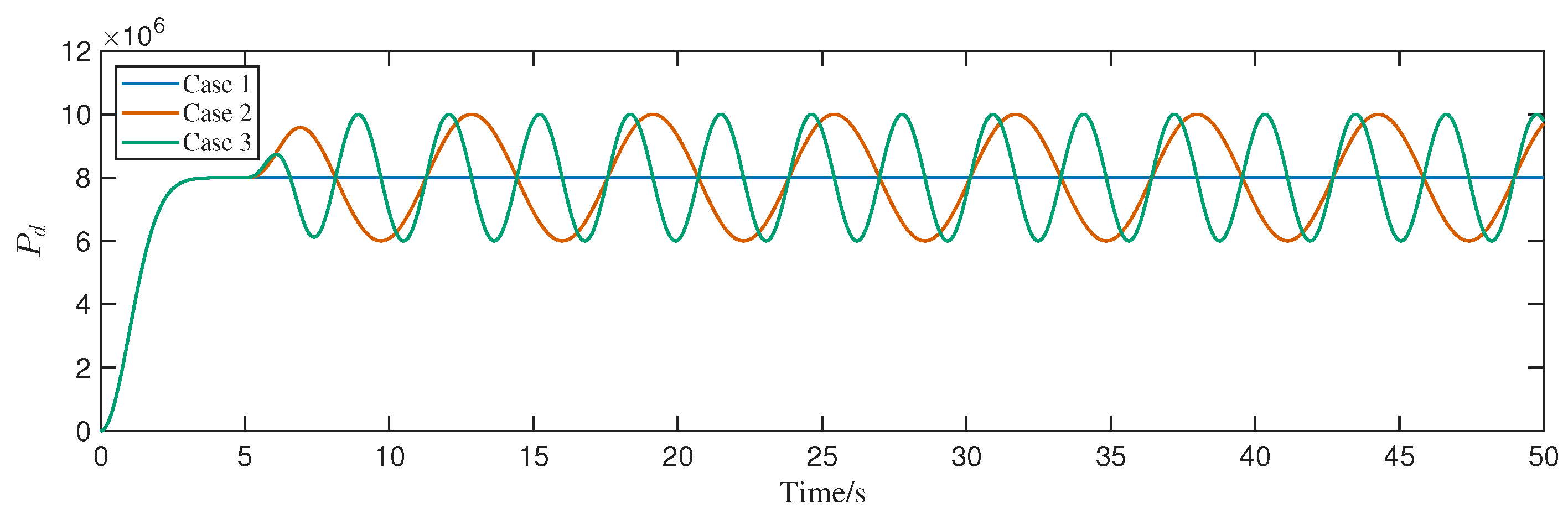
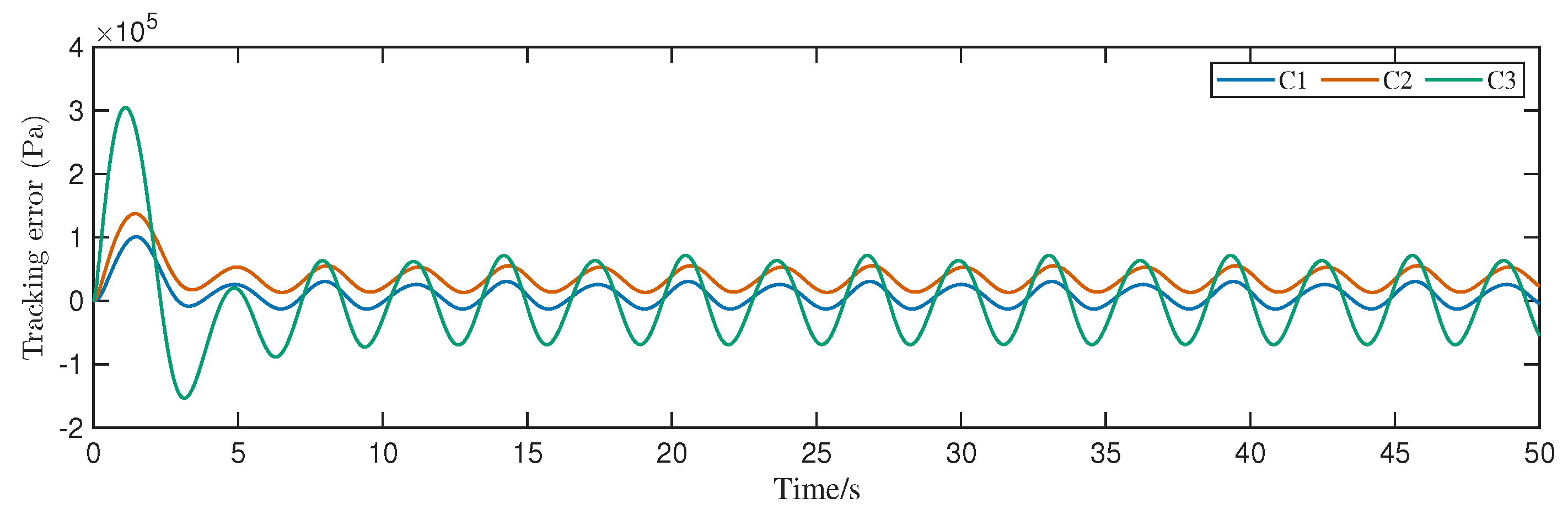
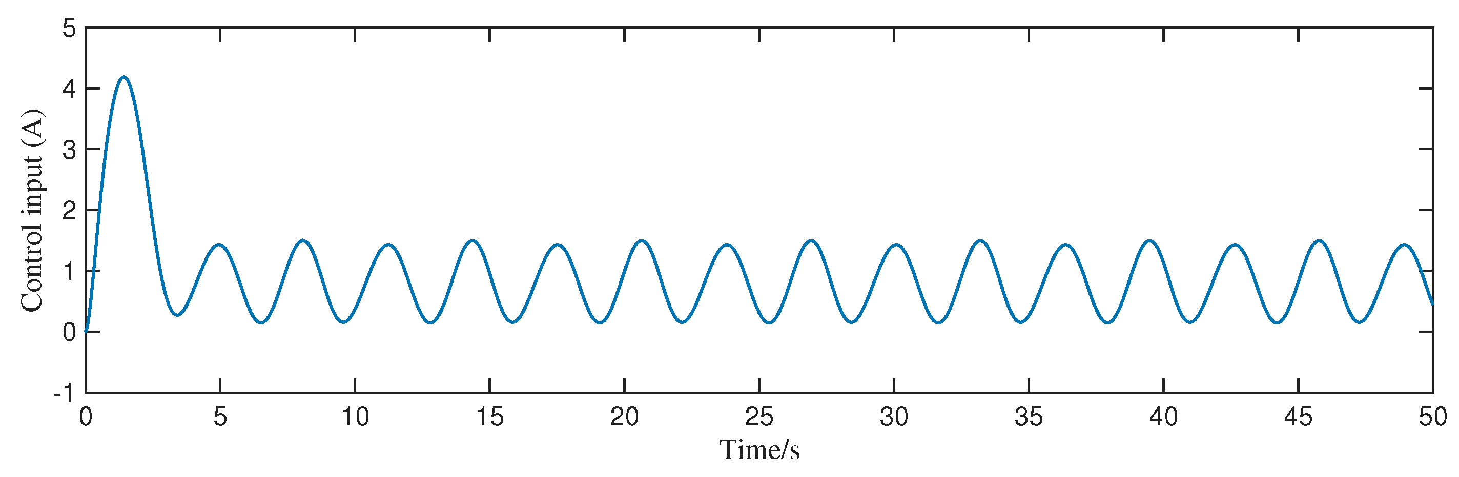
Case 1: The desired pressure is set as an approximately ramp-like signal, i.e., $x_{1d}=8\times {10}^6(1-exp(-0.5t^2))$, as shown in Figure 3. The pressure tracking errors of the three controllers are compared in Figure 4. It can be observed that C1 achieves the smallest tracking error among the three controllers because the nonlinear model information is utilized for feedforward compensation. C2 provides the second-best performance, since it retains the backstepping feedback structure but does not include detailed model-based compensation. In contrast, C3 does not use any model information and therefore exhibits the largest tracking error. These results demonstrate the effectiveness of the proposed model-based backstepping controller. Moreover, the comparison between C1 and C2 indicates that more accurate model information contributes to improved pressure tracking performance, which provides a useful insight for RDDPV pressure control. The comparison between C2 and C3 further shows that, even without detailed nonlinear model compensation, the controller constructed under the backstepping framework can still achieve relatively satisfactory tracking performance. Furthermore, the control input of C1 and the corresponding spool displacement are shown in Figure 5 and Figure 6, respectively. It can be observed that the control input remains continuous and bounded during the entire tracking process, and the spool displacement stays within the allowable physical range. In addition, the maximum value $M_Z$, mean value $A_Z$, and standard deviation $S_Z$ of the absolute tracking error in the last 20 s are calculated to quantify the steady-state tracking performance. The control input is also quantified by the accumulated quadratic cost $J={\int }_0^T{\displaystyle \frac{1}{2}}{i}^2\left(t\right)dt$. The corresponding results are listed in

Table 2. Quantitative comparison of tracking performance and control effort in Case 1.

Controller	${\mathit{M}}_{\mathit{Z}}$ (MPa)	${\mathit{A}}_{\mathit{Z}}$ (MPa)	${\mathit{S}}_{\mathit{Z}}$ (MPa)	J
C1	0.0305	0.0140	0.0086	65.2914
C2	0.0553	0.0342	0.0143	65.4078
C3	0.0716	0.0429	0.0210	67.3811

. It can be seen that C1 achieves the best performance among the three controllers in all these quantitative indices.

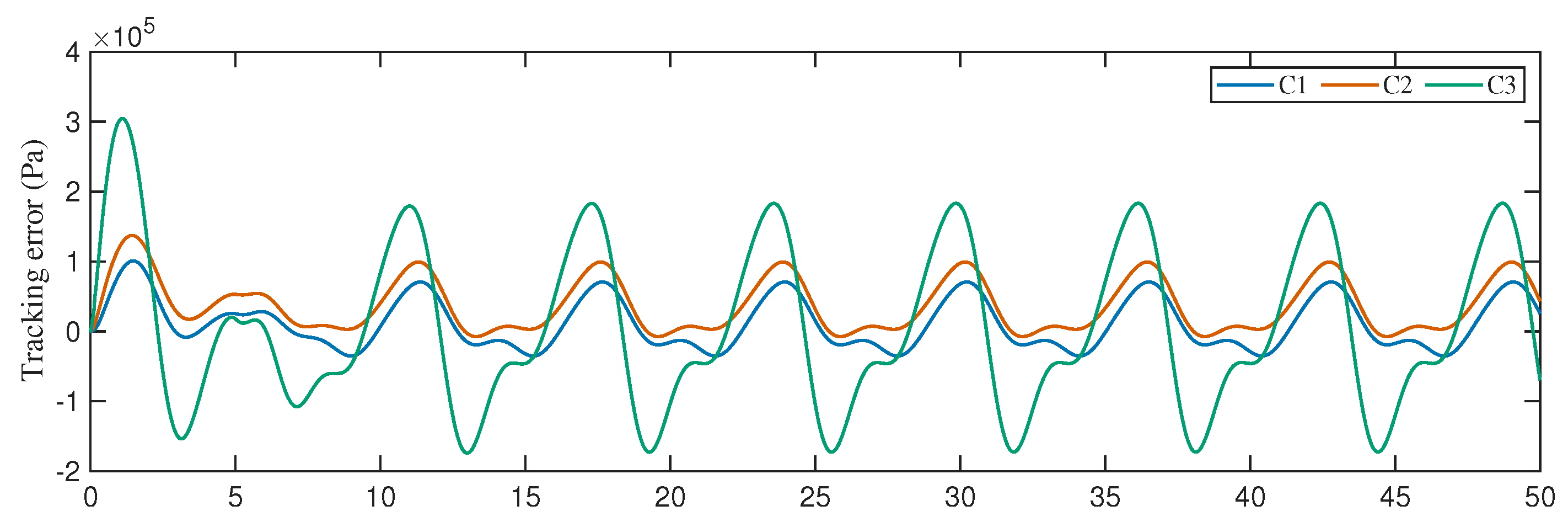
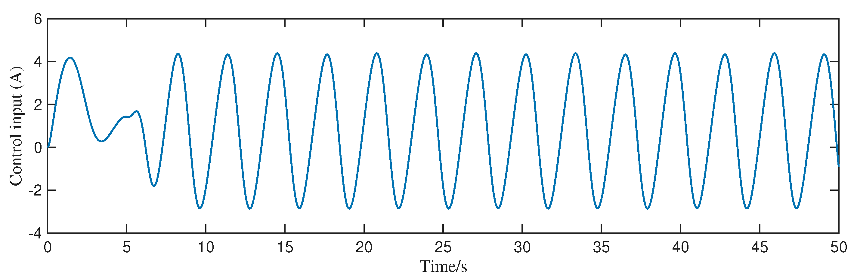
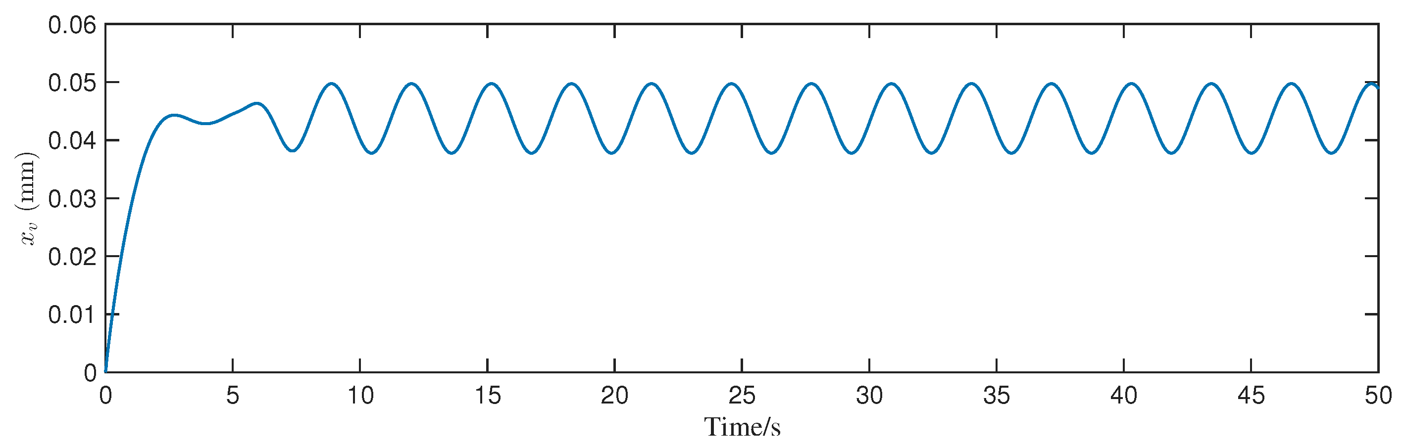
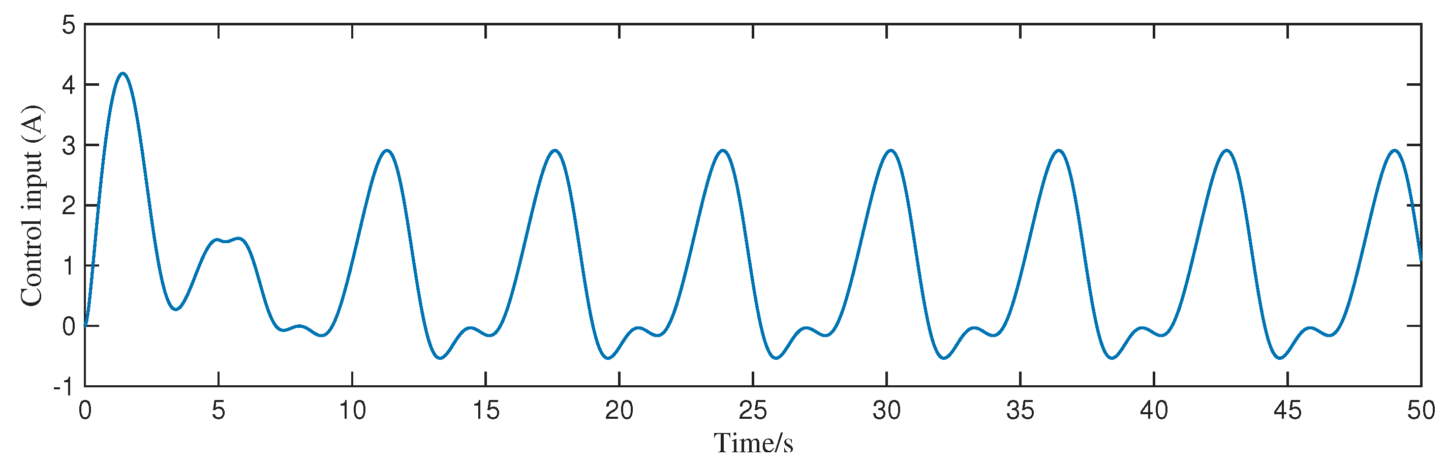
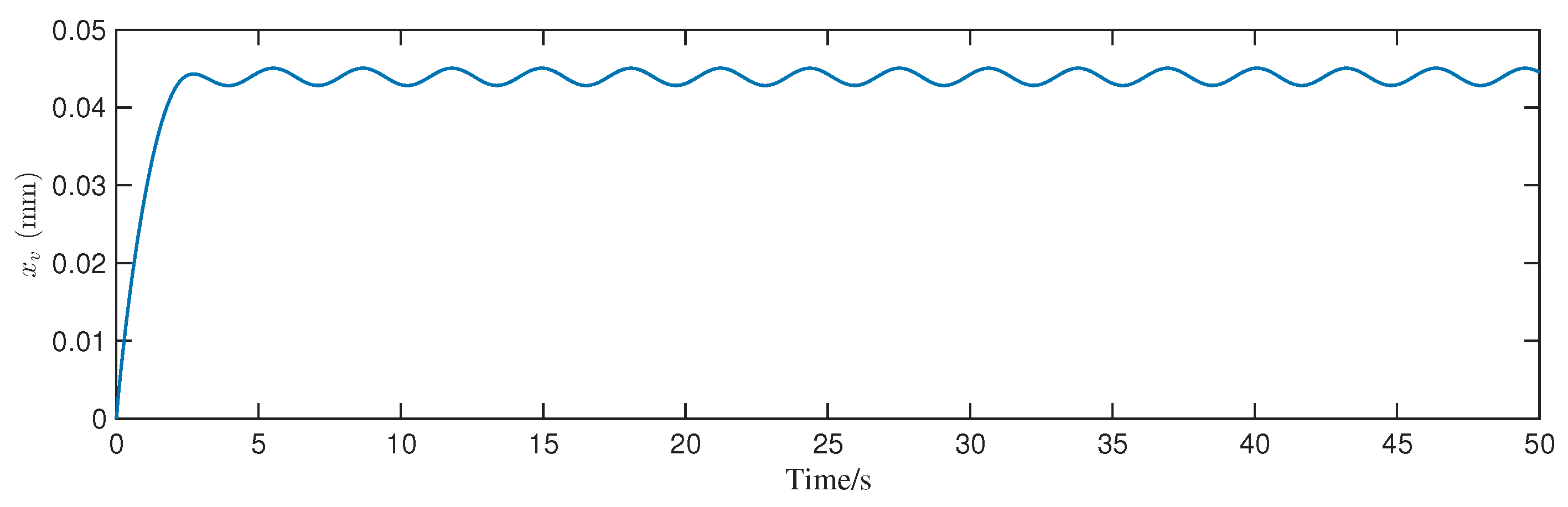
Case 2: To further compare the performance of the three controllers under a time-varying reference, a sinusoidal variation with an amplitude of $2\mathrm{MPa}$ is applied after the desired pressure reaches approximately $8\mathrm{MPa}$. The desired pressure trajectory is shown in Figure 3, and the corresponding tracking errors of the three controllers are shown in Figure 7. Due to the sinusoidal variation of the reference pressure, the tracking errors of all three controllers increase to some extent compared with Case 1. Nevertheless, C1 still maintains the smallest tracking error, C2 shows moderate tracking performance, and C3 exhibits the largest error among the three controllers. The control input and spool displacement of C1 are further shown in Figure 8 and Figure 9, respectively. It can be seen that both signals remain stable and bounded during the tracking process. In addition, the quantitative indices for Case 2 are listed in

Table 3. Quantitative comparison of tracking performance and control effort in Case 2.

Controller	${\mathit{M}}_{\mathit{Z}}$ (MPa)	${\mathit{A}}_{\mathit{Z}}$ (MPa)	${\mathit{S}}_{\mathit{Z}}$ (MPa)	J
C1	0.0707	0.0315	0.0206	116.0679
C2	0.0993	0.0375	0.0359	116.6273
C3	0.1831	0.0963	0.0564	123.7812

. It can be observed that C1 achieves the best performance among the three controllers in terms of both tracking accuracy and control effort.

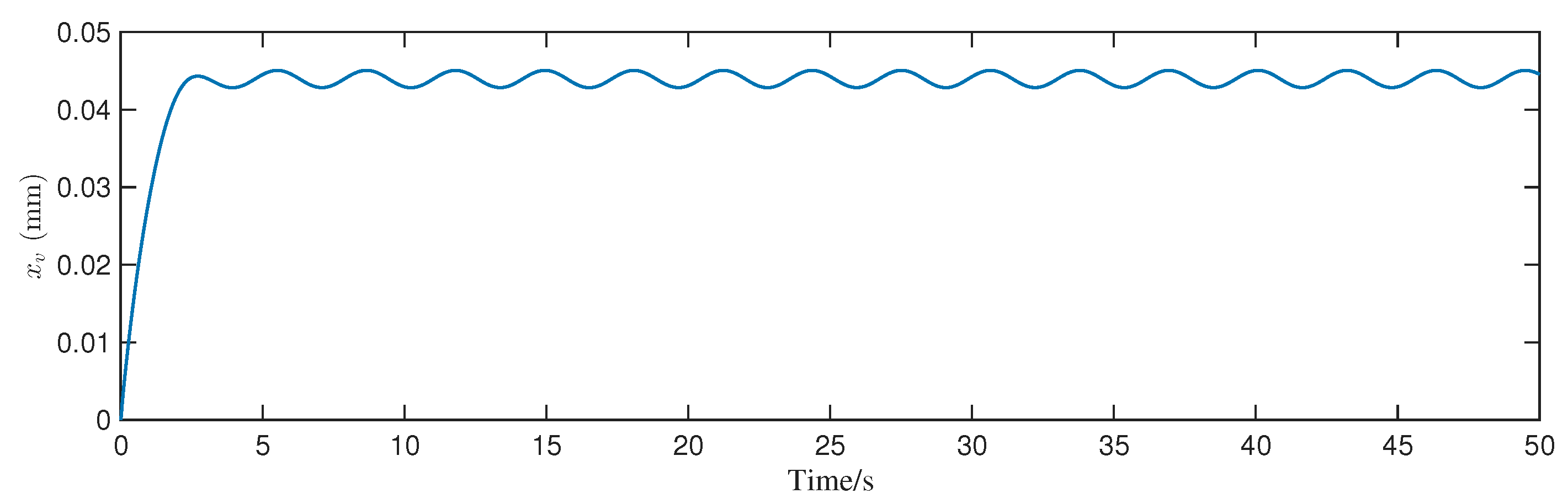
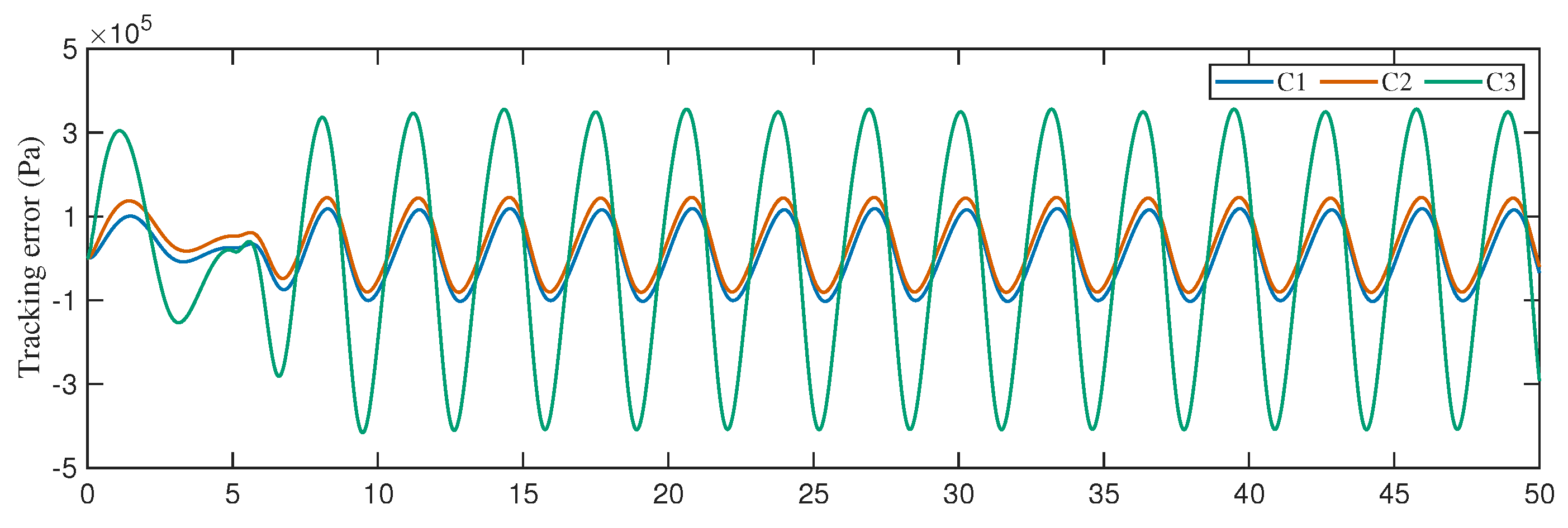
Case 3: To evaluate the tracking performance of the three controllers under a faster time-varying reference, the sinusoidal frequency in Case 2 is doubled while the pressure amplitude remains unchanged. The desired pressure trajectory is shown in Figure 3, and the corresponding tracking errors of the three controllers are presented in Figure 10. Compared with Case 2, the increased reference frequency imposes higher requirements on the dynamic response capability of the controllers, resulting in larger tracking errors for all three methods. Nevertheless, C1 still achieves the smallest tracking error owing to the use of model-based compensation, followed by C2, while C3 exhibits the largest tracking error. The control input and spool displacement of C1 are shown in Figure 11 and Figure 12, respectively. It can be observed that both signals remain bounded during the tracking process, indicating that the proposed controller can maintain stable operation under the faster reference variation considered in this case. In addition, the quantitative indices for Case 3 are listed in

Table 4. Quantitative comparison of tracking performance and control effort in Case 3.

Controller	${\mathit{M}}_{\mathit{Z}}$ (MPa)	${\mathit{A}}_{\mathit{Z}}$ (MPa)	${\mathit{S}}_{\mathit{Z}}$ (MPa)	J
C1	0.1189	0.0697	0.0347	333.1244
C2	0.1456	0.0756	0.0433	334.2458
C3	0.4090	0.2366	0.1179	381.6213

. It can be observed that C1 still achieves the best performance among the three controllers in terms of both tracking accuracy and control effort under the faster time-varying reference.

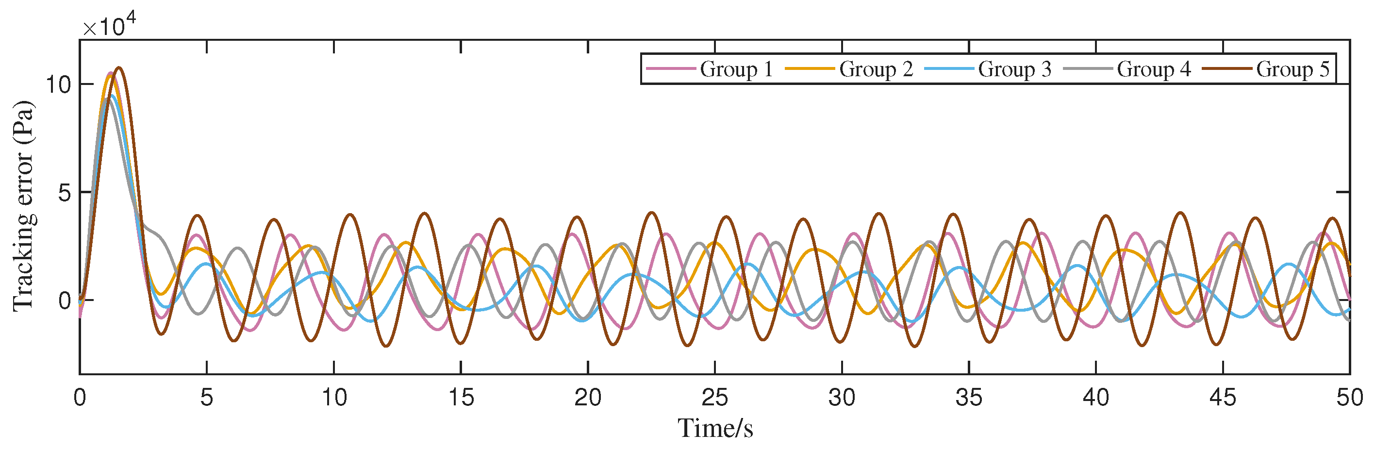
Case 4: To further evaluate the robustness of the proposed controller under model parameter uncertainties and disturbance variations, an additional robustness test is conducted based on the pressure reference trajectory in Case 1. This trajectory represents a typical pressure build-up process in practical braking applications. Different from the previous deterministic cases, five groups of randomized plant parameters and disturbances are considered in this case. The randomized parameters are generated using a Monte Carlo-style uniform sampling method. Specifically, the main uncertain mechanical and hydraulic parameters, including m, $B_v$, $k_v$, $J_r$, $B_r$, and E, are randomly selected within $\pm 30\%$ of their nominal values. Meanwhile, the disturbances are generated in the form of $d_1=A_{1}sin({\omega }_{1}t+{\varphi }_1)$ and $d_3=A_{3}sin({\omega }_{3}t+{\varphi }_3)$, where the disturbance amplitudes and frequencies are randomly varied around their nominal settings, and the disturbance phases are randomly selected within one full period. It should be emphasized that the randomization is applied only to the plant parameters and external disturbances. The proposed controller C1 is adopted in all five tests. The controller gains and the nominal model parameters used in the controller are kept unchanged throughout all five tests, while only the plant parameters and external disturbances are randomized. The five groups of randomized model and disturbance parameters are listed in

Table 5. Randomized model and disturbance parameters.

Parameter	Group 1	Group 2	Group 3	Group 4	Group 5
m	$4.244\times {10}^{-3}$	$4.904\times {10}^{-3}$	$5.339\times {10}^{-3}$	$6.331\times {10}^{-3}$	$6.038\times {10}^{-3}$
$B_v$	1.067	1.428	1.538	0.869	1.348
$k_v$	9023.85	11,558.60	7160.75	10,545.60	11,099.98
$J_r$	$2.04\times {10}^{-4}$	$1.32\times {10}^{-4}$	$1.75\times {10}^{-4}$	$1.59\times {10}^{-4}$	$1.21\times {10}^{-4}$
$B_r$	$2.57\times {10}^{-4}$	$2.69\times {10}^{-4}$	$3.40\times {10}^{-4}$	$2.48\times {10}^{-4}$	$2.31\times {10}^{-4}$
E	$1.442\times {10}^9$	$1.473\times {10}^9$	$1.506\times {10}^9$	$1.388\times {10}^9$	$1.087\times {10}^9$
$A_1$	$2.377\times {10}^7$	$1.808\times {10}^7$	$1.419\times {10}^7$	$1.430\times {10}^7$	$1.986\times {10}^7$
${\omega }_1$	1.702	1.550	1.473	2.073	2.112
${\varphi }_1$	1.687	2.291	2.319	3.281	6.207
$A_3$	0.604	0.481	0.509	0.465	0.437
${\omega }_3$	3.390	3.628	2.361	2.134	2.733
${\varphi }_3$	2.836	2.781	5.910	2.430	0.027

.

The tracking errors of C1 under the five randomized parameter and disturbance conditions are shown in Figure 13. Despite the variations in plant parameters and disturbance profiles, all five tracking error curves remain bounded during the entire pressure tracking process. The main tracking error appears in the initial pressure build-up stage, which is caused by the rapid increase in the desired pressure. After this transient stage, the pressure tracking errors settle into bounded small-amplitude oscillations and remain at a relatively low level for all randomized groups. Since the controller gains and the nominal model parameters are kept unchanged in all tests, the results demonstrate that the proposed controller can maintain satisfactory tracking performance under randomized model parameter mismatch and disturbance variations. This further supports the robustness of the proposed method under the considered operating conditions.

5. Conclusions

This paper investigates the application of a model-based backstepping control strategy to pressure regulation of the rotary direct-drive pressure valve (RDDPV). This research is motivated by the need for accurate braking pressure regulation in aircraft braking systems. Although the RDDPV has advantages in terms of structural simplicity, reduced size and weight, and improved anti-contamination capability, its pressure control is challenging due to the coupled motor-spool-pressure dynamics and hydraulic nonlinearities. To address this problem, a nonlinear dynamic model of the RDDPV is established, and a model-based backstepping pressure controller is developed by using nonlinear model information for feedforward compensation. Dynamic surface control is introduced to avoid direct differentiation of virtual control signals. The Lyapunov analysis shows that the closed-loop tracking errors are uniformly ultimately bounded under bounded disturbances. Comparative simulations under the tested reference pressure trajectories show that the proposed controller achieves better tracking performance than the controller without detailed model compensation and the conventional PI controller. Simulations with randomized model parameters and disturbance conditions further indicate that the proposed controller can maintain bounded tracking errors and acceptable control effort in the tested cases. These simulation results suggest the potential effectiveness of model-based nonlinear control for RDDPV pressure regulation under the considered operating conditions. Future work will focus on experimental verification on an RDDPV test platform and further investigation under practical aircraft braking load conditions.