Article

Fixed-Time Tracking Control for Underactuated Quadrotor UAVs with User-Defined Time Constraints

1
School of Automation, Jiangsu University of Science and Technology, Zhenjiang 212100, China
2
Department of Precision Instrument, Tsinghua University, Beijing 100084, China
*
Authors to whom correspondence should be addressed.
Actuators 2026, 15(5), 270; https://doi.org/10.3390/act15050270
Submission received: 8 April 2026 / Revised: 30 April 2026 / Accepted: 5 May 2026 / Published: 9 May 2026

Abstract

This paper investigates the fixed-time tracking control problem for underactuated quadrotor unmanned aerial vehicle systems subject to mass parameter uncertainties and user-defined time constraints. For the parameter uncertainties inherent in the system, the approximation capability of neural networks is exploited for compensation. Combined with the backstepping technique, this work proposes a new adaptive control strategy to ensure that the error variable converges within a small region near zero within a fixed time, and the designed controller effectively avoids singularity issues. Furthermore, a unified constraint framework with a shift function is introduced into the controller design, thereby providing a unified framework for user-defined time constraints that can flexibly handle different constraint scenarios without altering the control architecture. Finally, simulations are conducted to validate the effectiveness of the proposed method.

1. Introduction

In recent years, unmanned aerial vehicles (UAVs), particularly quadrotor platforms, have garnered significant attention in both academic and industrial communities due to their exceptional maneuverability, hovering capability, and vertical takeoff and landing characteristics [1,2]. As a typical underactuated Euler–Lagrange system, quadrotors possess six degrees of freedom but only four independent control inputs, resulting in strong nonlinear coupling between translational and rotational dynamics. This underactuated structure, combined with aerodynamic effects and intrinsic nonlinearities, poses inherent challenges for controller design. During practical missions, such as inspection, reconnaissance, disaster relief, and cooperative transportation, UAVs inevitably encounter parameter variations, modeling uncertainties, and external disturbances including wind gusts and turbulent airflow. To cope with these uncertainties, adaptive control and neural networks (NNs) approximation techniques have been widely employed in nonlinear and UAVs systems [3,4,5,6,7,8,9]. In addition, minimum-time reference generation with energy consideration [10] and sliding mode-based robust control [11] have also been studied for UAVs performance improvement. Nevertheless, designing robust and high-performance tracking control strategies for uncertain underactuated quadrotor systems remains a fundamental and challenging research problem.
Among various control performance metrics, convergence speed plays a critical role in UAVs applications, especially in time-sensitive tasks such as emergency response, agile maneuvering, and dynamic target tracking. Traditional asymptotic control methods only guarantee convergence as time approaches infinity and therefore cannot satisfy stringent rapid-response requirements. Finite-time control improves transient performance by ensuring convergence within a finite time horizon. For instance, finite-time consensus and tracking control strategies were investigated in [3,12,13,14,15] and an overview of finite-time control in UAVs systems was presented in [16]. Sliding-mode-based finite-time control methods have also been applied to aerial vehicles systems [17]. However, the settling time of finite-time control typically depends on initial conditions, limiting predictability under uncertain initial states. To eliminate this limitation, fixed-time stability theory was introduced in [18], where convergence time is independent of initial conditions and solely determined by control parameters. Following this concept, fixed-time control approaches have been widely studied for trajectory tracking of UAVs systems [19,20,21,22,23]. In UAVs applications, singularity-free and predefined-performance-based fixed-time control schemes were further investigated in [24,25,26,27]. Despite these advances, applying fixed-time control to uncertain underactuated quadrotor systems still presents several challenges. First, fixed-time stability conditions often involve nonlinear power-law terms that may induce singularities in controller implementation [22,25]. Second, the strong coupling between position and attitude subsystems increases the complexity of fixed-time stability analysis. Third, fixed-time convergence properties must be preserved while maintaining robustness against unknown disturbances.
Beyond convergence performance and robustness, practical UAVs operations frequently require state constraints to ensure safety and mission compliance. For instance, during low-altitude flight or navigation in confined environments, position states must remain within prescribed bounds to prevent collisions or structural damage. Classical constraint-handling approaches—particularly those based on the Barrier Lyapunov Function (BLF)—have been widely applied to nonlinear systems with state constraints. Distributed adaptive tracking with state constraints was studied in [28], while event-triggered robust tracking control for Euler–Lagrange systems with full-state constraints was developed in [29]. Cao et al. introduced a comprehensive constraint function in [30] to limit tracking errors, a method equally capable of handling unconstrained scenarios. The introduction of this comprehensive constraint function not only expands the scope of constrained control problems but also enhances the flexibility and applicability of control system design. And neural-network-based constrained adaptive control schemes were further investigated in [31,32,33,34,35]. However, most existing methods assume that constraints remain active throughout the entire operation. In many realistic UAVs tasks, constraints are activated only during specific mission intervals rather than throughout the whole process. Directly applying traditional BLF methods to user-defined time constraints (UTCs) scenarios may cause discontinuities or require controller restructuring during phase transitions, thereby increasing implementation complexity and potentially affecting system stability. Moreover, integrating constraint-handling mechanisms with fixed-time stability analysis further complicates controller design due to the nonlinear interaction between constraint functions and fixed-time Lyapunov conditions.
To address the aforementioned challenges, this paper proposes an adaptive neural network-based fixed-time control strategy for underactuated quadrotor UAVs subject to uncertainties, disturbances, and UTCs. The main contributions and innovations are summarized as follows:
(1) An adaptive fixed-time tracking control algorithm is designed using backstepping and neural network techniques to ensure tracking errors converge to a near-zero compact set within a fixed-time, with convergence time upper bound estimation independent of initial condition, while avoiding singularity issues commonly encountered in conventional fixed-time controller designs [22,25].
(2) A unified constraint framework incorporating a fusion transformation mechanism is developed to handle UTCs. Unlike traditional BLF-based constraint methods [28,29,30], the proposed unified framework seamlessly accommodates constrained and unconstrained phases without altering the controller structure. Furthermore, symmetric, asymmetric, and prescribed constraint forms are naturally included as special cases, enabling adaptation to diverse task-dependent constraint requirements.

2. Preliminaries

2.1. Notations

Throughout this paper, R n denotes the n-dimensional Euclidean space and R m × n denotes the space of real m × n matrices. The set of positive real numbers is denoted by R + . Old lowercase letters represent vectors, while bold uppercase letters denote matrices. The transpose of a matrix is indicated by the superscript · T . The Euclidean norm of a vector x R n is defined as x = x T x . For a symmetric matrix A, λ min ( A ) and λ max ( A ) denote its minimum and maximum eigenvalues, respectively. I denotes the identity matrix of compatible dimensions. The operators max ( · ) and min ( · ) denote the maximum and minimum values, respectively. For any vector a R 3 , S ( a ) R 3 × 3 denotes the associated skew-symmetric matrix satisfying S ( a ) b = a × b for all b R 3 , where × represents the cross product. The skew-symmetric matrix satisfies the properties S ( a ) T = S ( a ) , a T S ( a ) b = 0 and S ( a ) 2 = a a T a 2 I . Moreover, the following triple product identity holds: a T S ( b ) c = ( a × b ) · c = b T S ( c ) a = c T S ( b ) a . In particular, for a unit vector a, it holds that S ( a ) 2 = a a T I . For any rotation matrix R S O ( 3 ) , the following identity holds R S ( a ) R T = S ( R a ) , which implies that the cross product is invariant under rotation, i.e., R ( a × b ) = ( R a ) × ( R b ) . The special orthogonal group is defined as S O ( 3 ) : = { D R 3 × 3 D T D = I , det ( D ) = 1 } . The unit sphere in R 3 is denoted by S ( 2 ) : = { x R 3   x   = 1 } . The unit vector along the positive z-axis is denoted by e 3 : = [ 0 , 0 , 1 ] T . The operator diag ( · ) denotes a diagonal matrix formed by the corresponding elements. For a time-dependent scalar or vector function f ( t ) , f ˙ ( t ) denotes its time derivative. A symmetric matrix A is said to be positive definite, denoted by A > 0 , if x T A x > 0 for all x 0 .

2.2. Coordinate Frames and Vehicle Modeling

To facilitate the subsequent controller design and stability analysis, the coordinate frames and principal force directions of the quadrotor unmanned aerial vehicle are first introduced. Figure 1 illustrates the geometric configuration of the system, including the inertial frame, the body-fixed frame, the position vector, and the thrust-related directions. This geometric description provides the foundation for the dynamic model developed in this subsection.
As shown in Figure 1, we use I as the inertial frame and B as the body-fixed frame, where the origin of B is located at the UAV’s center of mass. The kinematic and dynamic equations describing vehicle motion are given by [2]
p ˙ = ν , ν ˙ = 1 m f + g e 3 + d , R ˙ = R S ( Ω ) J Ω ˙ = S ( Ω ) J Ω + τ
where p R 3 and ν R 3 represent the position vector and velocity vector in the inertial frame, respectively. m R denotes the drone’s mass. f R 3 indicates thrust in the I . g R signifies gravitational acceleration. e 3 = 0 , 0 , 1 T is a unit vector pointing along the positive z-axis direction. R S O ( 3 ) is the rotation matrix. Ω R 3 represents the angular velocity in the B . d R 3 denotes external disturbances in the I , such as wind. J R 3 × 3 is the moment of inertia matrix. τ R 3 represents the control torque.
For a quadrotor platform, the total aerodynamic thrust is generated only along the body-fixed frame vertical direction and this force is normal to the rotor plane. Under this configuration, the resultant force can be represented as follows:
f = T R e 3 ,
where T : = f corresponds to the total thrust of the four rotors, whose direction is given by r 3 S ( 2 ) , with
r 3 : = R e 3 .
To achieve specific maneuvers, a desired thrust vector f d R 3 is introduced, which is specified as follows:
f d = T d r 3 d ,
where T d : = f d represents the desired net thrust applied along direction r 3 d S ( 2 ) . Therefore, the required thrust direction is calculated as
r 3 d : = 1 T d f d S 2 .
Intuitively, r 3 d specifies the desired thrust direction of f . As the actual thrust T can only act along r 3 , it is chosen as T = T d r 3 d T r 3 . With the aid of (2) and (5), we obtain f = r 3 r 3 T f d . With r 3 r 3 T = I + S 2 ( r 3 ) , it can be deduced that
f = f d T d S 2 ( r 3 ) r 3 d .
The direction r 3 d cannot be arbitrarily assigned, as it is dictated by the stabilizing force f.

2.3. Problem Statement and Control Objective

Consider a reference trajectory p d ( t ) R 3 , defined for all t t 0 , which belongs to class C 2 . Its first- and second-order derivatives, p ˙ d ( t ) and p ¨ d ( t ) , are assumed to be bounded. We set x 1 = p , x 2 = ν . Let us define the position and velocity errors as
z 1 t = x 1 t p d t ,
z 2 ( t ) = x 2 ( t ) α ( t ) ,
where z 1 represents position error, and z 2 represents velocity error. Among them, α is a virtual controller.
This work considers applying UTCs to x 1 s ( t ) ( s = 1 , , n ) during [ t a , t f ) , where t a and t f correspond to the activation and termination times, respectively, satisfying 0 t 0 < t a < t f . The UTCs scheme is described below:
(1)
During [ t 0 , t a ) or [ t f , + ) , x 1 s ( t ) imposes no constraints.
(2)
During [ t a , t f ) , x 1 s ( t ) constrained by the custom constraint set
Ξ ( t ) : = x 1 s ( t ) R L ̲ s ( t ) < x 1 s ( t ) < L ¯ s ( t ) , t [ t a , t f ) ,
where L ̲ s ( t ) and L ¯ s ( t ) correspond to the lower and upper time-varying bounds of x 1 s ( t ) .
Purpose of this paper: For underactuated quadrotor UAVs systems, uncertainties in mass-related parameters and external disturbances exist. Based on this, the control objectives of this work are defined as follows:
(1)
All errors converge to a compact set within a fixed time;
(2)
x 1 s ( t ) ( s = 1 , , n ) follows UTCs.
Assumption 1.
The position state of the UAV must satisfy J ̲ s x 10 s ( t ) J ¯ s , where J ̲ s and J ¯ s represent predetermined constants, and satisfy L ̲ s ( t ) > J ̲ s and L ¯ s ( t ) > J ¯ s .
Remark 1.
For practical tracking, the constraints imposed on the follower should be no less restrictive than those of the reference trajectory. Accordingly, Assumption 1 requires L ̲ s ( t ) > J ̲ s and L ¯ s ( t ) > J ¯ s .
Remark 2.
Assumption 1 is a standard feasibility condition for the proposed barrier-type user-defined time constraint (UTC) framework. Specifically, during the active constraint interval t [ t a , t f ) , the transformed error should satisfy W s ( t ) < β s ( t ) < W ¯ s ( t ) , s = 1 , , n , so that the variable λ s ( t ) in (11) is well defined. Under this admissible-domain condition and continuous closed-loop state evolution, the boundedness of λ s ( t ) prevents β s ( t ) from reaching the constraint boundary, thereby ensuring constraint preservation. However, if an extreme instantaneous perturbation, such as a physical impact, causes a discontinuous jump of the UAV position and leads to β s ( t + ) ( W s ( t + ) , W ¯ s ( t + ) ) , the barrier transformation is no longer valid after the impact, and the Lyapunov-based stability proof cannot directly guarantee constraint satisfaction from this infeasible state. In practice, the UAV may remain bounded under actuator and system limits, but the strict state-constraint guarantee is temporarily lost. Such events should be handled by a supervisory safety mechanism, e.g., emergency hovering/landing, constraint-envelope re-planning, or reference resetting, to restore feasibility. Once the post-impact state is back in the admissible set, the proposed fixed-time adaptive controller can resume ensuring tracking performance while respecting the updated constraints.

2.4. Shift Function and Unified Constraint Framework

The UTCs framework consists of two unconstrained phases and one constrained phase, where the constraint is activated over a specified time interval. The transition between these phases is discontinuous. To handle this discontinuity, a shift function is introduced as follows:
χ s ( t ) = exp tan π t a t 2 t a 2 p 2 ( ω 1 s ) 2 p , t [ t 0 , t a ) 1 , t [ t a , t f ) exp ( t t f ) 2 p 2 ( ω 2 s ) 2 p , t [ t f , + )
where ω 1 s R + , ω 2 s R + , p denotes the order of the system.
Property 1.
The shift function (10) possesses the following characteristics:
(1) 
In the [ t 0 , t a ) stage, χ s ( t ) monotonically increases, and lim t t a χ s ( t ) = 1 .
(2) 
χ s ( t ) reaches 1 at t = t a and maintains χ s ( t ) = 1 during phase [ t a , t f ) .
(3) 
In the [ t f , + ) stage, χ s ( t ) monotonically decreases, and lim t + χ s t = 0 .
(4) 
χ ˙ s ( t ) is continuous.
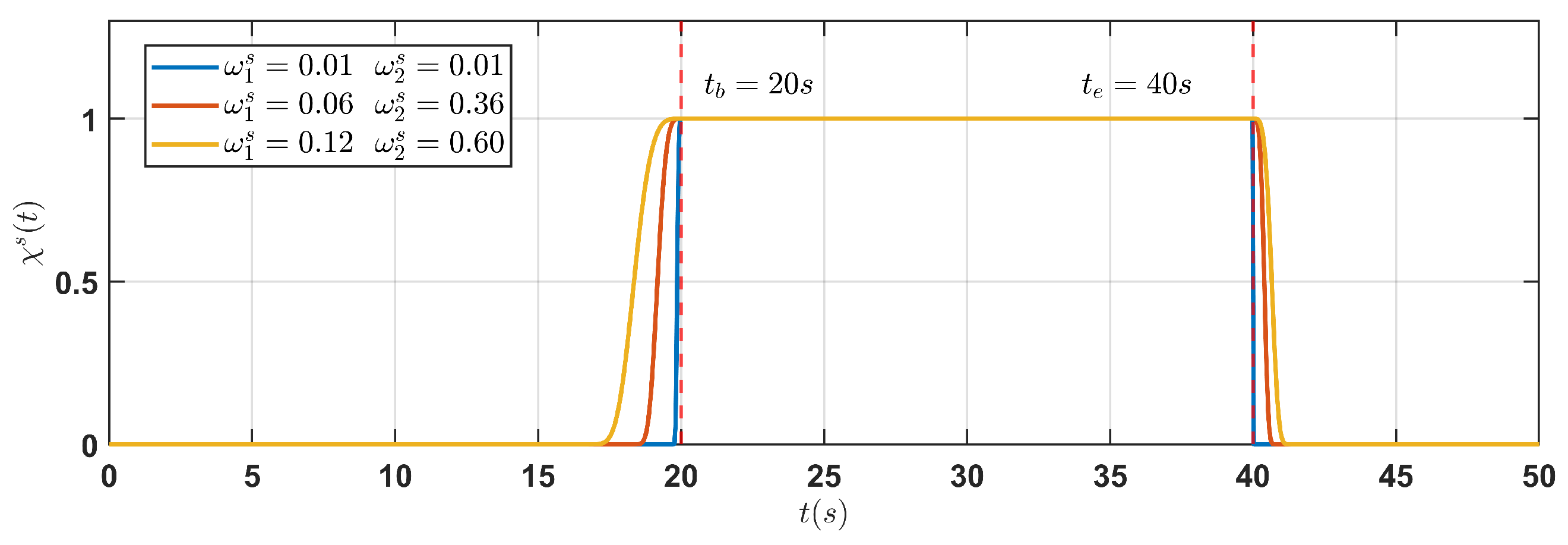
Since Property 1 is easily verifiable, its proof is omitted. It is important to emphasize that in the shift function (10), ω 1 s and ω 2 s govern the growth and decay rates of χ s ( t ) . As observed in Figure 2, the smaller ω 1 s leads to a faster increase in χ s ( t ) toward 1, while the smaller ω 2 s results in a quicker convergence toward zero. These characteristics ensure that the shift function χ s ( t ) shifts smoothly across constrained and unconstrained regimes while maintaining continuity.
To impose UTCs on the position state x 1 s ( t ) ( s = 1 , , n ) in a UAV system, constraints must first be applied to the position tracking error z 1 s , inspired by the BLFs framework. Subsequently, the following unified constraint framework is formulated:
λ s ( t ) = W ̲ s ( t ) W ¯ s ( t ) z 1 s ( t ) W ̲ s ( t ) + β s ( t ) W ¯ s ( t ) β s ( t )
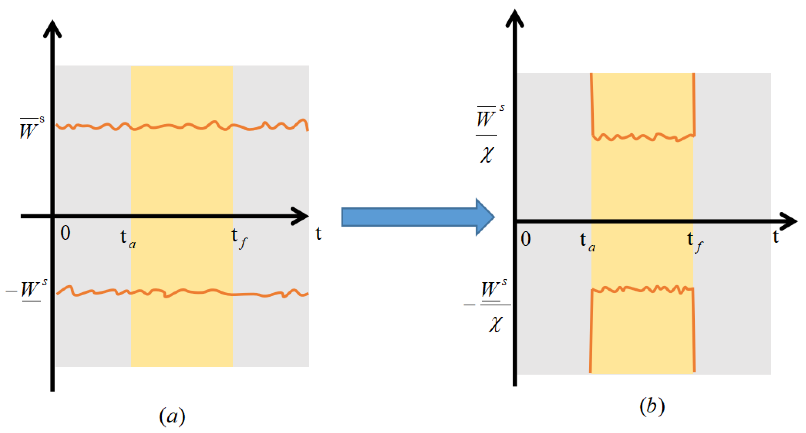
where β s ( t ) = χ s ( t ) z 1 s ( t ) , the position tracking error z 1 s ( t ) is further discussed in the next section on fixed-time local tracking control algorithm design, β s ( 0 ) W ̲ s ( 0 ) , W ¯ s ( 0 ) , while W ̲ s ( t ) and W ¯ s ( t ) denote the lower bound and upper bound of the constraint function of z 1 s ( t ) . Clearly, if β s ( t ) W ̲ s ( t ) or β s ( t ) W ¯ s ( t ) , right then λ s ( t ) ± , and only when β s = 0 holds, λ s = 0 . Therefore, when λ s ( t ) remains bounded under the designed controller, W ̲ s ( t ) < β s ( t ) < W ¯ s ( t ) can be guaranteed. Combining (10), we can further deduce from (11) that λ s ( t ) ± holds if and only if z 1 s W ̲ s / χ s or z 1 s W ¯ s / χ s . Simultaneously, for t [ t 0 , t a ) or [ t f , + ) , if χ s 0 + holds, then W ̲ s / χ s and W ¯ s / χ s + hold, implying z 1 s ( t ) ( , ) , which means z 1 s ( t ) is unconstrained. When t [ t a , t f ) holds, χ s = 1 , follows from (10), subsequently implying W ̲ s < z 1 s < W ¯ s . This indicates that z 1 s ( t ) is constrained. For clarity, the principle of unified constraint framework is illustrated in Figure 3.
Differentiating λ s ( t ) yields
λ ˙ i s ( t ) = P 1 s ( t ) z ˙ 1 s ( t ) + P 2 s ( t ) χ ˙ s ( t ) + θ s ( t ) ,
where
P 1 s ( t ) = W ̲ s ( t ) W ¯ s ( t ) W ̲ s ( t ) W ¯ s ( t ) + β s ( t ) 2 W ̲ s ( t ) + β s ( t ) 2 W ¯ s ( t ) β s ( t ) 2 ,
P 2 s ( t ) = W ̲ s ( t ) W ¯ s ( t ) z 1 s ( t ) 2 W ¯ s ( t ) W ̲ s ( t ) 2 β s ( t ) W ̲ s ( t ) + β s ( t ) 2 W ¯ s ( t ) β s ( t ) 2 ,
θ s t = λ s ( t ) W ̲ s ( t ) W ̲ s ( t ) + λ s ( t ) W ¯ s ( t ) W ¯ ˙ s ( t ) ,
λ s ( t ) W ̲ s ( t ) = W ¯ s ( t ) β s ( t ) z 1 s ( t ) W ̲ s ( t ) + β s ( t ) 2 W ¯ s ( t ) β s ( t ) ,
λ s ( t ) W ¯ s ( t ) = W s ( t ) β s ( t ) z 1 s ( t ) W ̲ s ( t ) + β s ( t ) W ¯ s ( t ) β s ( t ) 2 .
Additionally, by adjusting specific time parameters t a and t f , flexible adjustment of constraint forms can be realized to suit diverse task requirements. The corresponding cases are described in the following:
Case 1: If t a = 0 , t f > 0 , this indicates an initial constraint scenario. This indicates that the constraint is active during the initial phase and is removed afterward. During the t > t f phase, due to χ s 0 + , it can be inferred that W ̲ s / χ s and W ¯ s / χ s + , indicating that this phase is unconstrained.
Case 2: If t a > 0 , t f = + , this corresponds to a delayed constraint scenario. This indicates that the constraint is applied to the system after a period following the start of the operation. During the phase of 0 < t < t a , it can be inferred that W ̲ s / χ s and W ¯ s / χ s + , since χ s 0 + , meaning this phase is unconstrained.
Case 3: If t a = 0 , t f = + , this indicates a continuous constraint scenario. This situation implies that the constraint is always applied, i.e., since t 0 , χ s = 1 holds, W ̲ s < z 1 s < W ¯ s is satisfied, which is analogous to the cases considered in existing results.
Case 4: If t a = t f = + , this indicates an unconstrained scenario. This situation signifies that the constraint is removed, meaning that due to χ s 0 + , for t > 0 , W ̲ s / χ s and W ¯ s / χ s + .
The above analysis demonstrates that the unified constraint framework (11) facilitates fixed-time tracking control of constrained UAVs systems.

2.5. Related Lemma

Lemma 1
([5]).  If Y R n × n is a symmetric positive definite matrix, then for x R n , the following inequality holds
λ min ( Y ) x 2 x T Y x λ max ( Y ) x 2 .
Lemma 2
([36]).  If ϕ , θ R , then the following inequality holds
ϕ · θ ε p p | ϕ | p + 1 q ε q | θ | q ,
where ε > 0 , p > 1 , q > 1 , ( p 1 ) ( q 1 ) = 1 .
Lemma 3
([37]).  If x n > 0 , n = 1 , , m and 0 < α 1 , then the following inequality holds
n = 1 m x n α n = 1 m x n α .
Lemma 4
([37]).  If x n > 0 , n = 1 , , m and α > 1 , then the following inequality holds
m 1 α · n = 1 m x n α n = 1 m x n α n = 1 m x n α .
Lemma 5
([38,39]).  Consider the following system x ˙ ( t ) = f ( t , x ) , x ( 0 ) = x 0 , where x R n , f : R + × R n R n and the origin is an equilibrium point. For m > 0 , n > 0 , 0 < q < 1 , p > 1 , if there exists a positive definite function U ( x ) satisfying U ( x ) m U q ( x ) n U p ( x ) , then the origin is fixed-time stable, and the upper bound estimate for the convergence time is
T T max = 1 m ( 1 q ) + 1 n ( p 1 ) .
Lemma 6
([40]).  Suppose that the signal x ( t ) and its first derivative are bounded. Consider the following linear system
δ ξ ˙ = ξ + x ( t ) .
Then, there exist positive constants c 1 , c 2 , and t * such that for all t t * .
ξ x ( t ) c 1 δ , ξ ˙ x ˙ ( t ) c 2 δ .
where ξ R 3 is the filter state, δ > 0 is a small positive constant, and · denotes the Euclidean norm. The constants c 1 , c 2 > 0 are independent of δ, and t * is a finite settling time. Moreover, the approximation error can be made arbitrarily small by selecting sufficiently small δ.

3. Controller Design and Stability Analysis

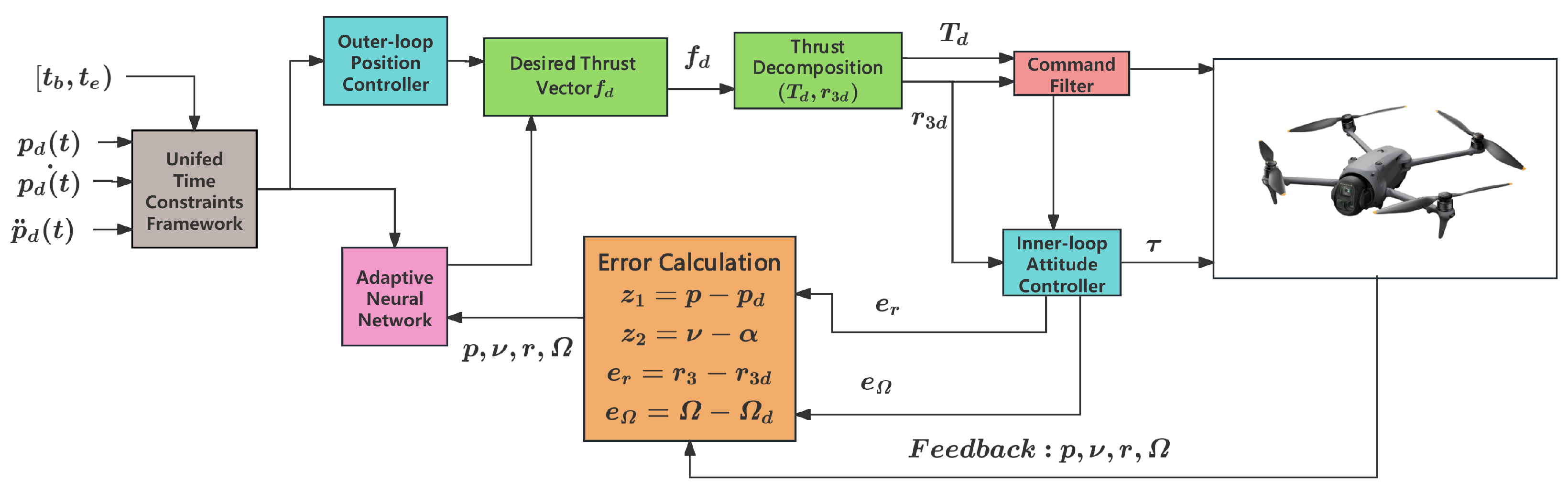
In subsequent sections, an adaptive backstepping algorithm is designed for UAVs systems. The overall control framework of the proposed method is shown in Figure 4.

3.1. Position Control

First, define position error and velocity error as
z 1 t = x 1 t p d t ,
z 2 ( t ) = x 2 ( t ) α ( t ) ,
where z 1 = [ z 1 1 , , z 1 n ] T R n represents position error, and z 2 = [ z 2 1 , , z 2 n ] T R n represents velocity error. Among them, α is a virtual controller. Using (13) and x ˙ 1 = x 2 = p ˙ = ν , x ˙ 2 = ν ˙ , taking the derivative of z 1 yields
z ˙ 1 = x 2 p ˙ d ,
where p ˙ d represents the derivative of p d . Furthermore, with the aid of (14), the time derivative of z 1 can be equivalently expressed as
z ˙ 1 = z 2 + α p ˙ d .
Based on the unified constraint framework (11) and its time derivative (12), it can be derived that
λ ˙ = P 1 z 2 p ˙ d + α + P 2 χ ˙ + θ ,
where P 1 = diag { P 1 1 , , P 1 n } , P 2 = diag { P 2 1 , , P 2 n } , θ = [ θ 1 , , θ n ] T , χ ˙ = [ χ ˙ 1 , , χ ˙ n ] T .
Subsequently, the virtual control law α is designed as follows:
α = P 1 1 K 11 1 2 3 4 Θ 1 ( λ ) K 12 1 2 2 λ λ T λ + P 1 p ˙ d P 2 χ ˙ θ
where the parameters K 11 R + and K 12 R + represent gain parameters, and the function Θ 1 ( λ ) is defined as follows:
Θ 1 ( λ ) = λ λ T λ 1 4 if λ ϖ 1 5 4 λ ϖ 1 1 2 1 4 λ λ T λ ϖ 1 5 2 otherwise
where ϖ 1 R + .
The first Lyapunov function is constructed as follows:
V 1 = 1 2 λ T λ .
Taking the time derivative of V 1 yields
V ˙ 1 = K 11 1 2 λ T λ 3 4 K 12 1 2 λ T λ 2 + λ T P 1 z 2 + ϑ 1 ,
where
ϑ 1 = 0 λ ϖ 1 K 11 1 / 2 3 4 Y 1 otherwise
Y 1 = λ T λ 3 4 5 4 λ T λ ϖ 1 1 2 + 1 4 λ T λ 2 ϖ 1 5 2 .
Remark 3.
Based on Boundary z 1   = ϖ 1 , it can be seen that
lim λ ϖ 1 λ λ T λ 1 4 = lim λ ϖ 1 λ     λ   1 2 = ϖ 1 1 2 λ ,
lim λ ϖ 1 ( 5 4 λ ϖ 1 1 2 1 4 λ λ T λ ϖ 1 5 2 ) = ϖ 1 1 2 λ .
Clearly, Item ϖ 1 1 2 λ concerns the continuity and differentiability of λ. Therefore, the piecewise function Θ 1 ( λ ) is continuously differentiable. It should be noted that the form of piecewise function Θ 1 ( λ ) is designed to circumvent singularity issues. Using (27), it is easy to obtain lim λ 0 Θ 1 ( λ ) = lim λ 0 5 / 4 λ ϖ 1 ( 1 / 2 ) 1 / 4 λ λ T λ ϖ 1 ( 5 / 2 ) = 0 . Furthermore, an extremely small value of ϖ 1 can result in a large value for the virtual controller, which may lead to failure of the control algorithm. Therefore, it is necessary to select an appropriate value of ϖ 1 to meet practical requirements.
The time derivative of the velocity error z 2 in (14) is derived to facilitate the design of the desired thrust vector f d . Therefore, the translational subsystem can be equivalently represented as m v ˙ = f + m g e 3 + m d .
Using (1) and (6), and taking the time derivative of z 2 , we obtain
z ˙ 2 = 1 m f d T d S 2 ( r 3 ) r 3 d + m d + m g e 3 α ˙ .
We construct the second Lyapunov function as follows:
V 2 = 1 2 z 2 T m z 2 .
The time derivative of V 2 in (22), using (21), is derived as
V ˙ 2 = z 2 T m z ˙ 2 + 1 2 z 2 T m ˙ z 2 = z 2 T f d T d S 2 ( r 3 ) r 3 d + m d + m g e 3 m α ˙ + 1 2 z 2 T m ˙ z 2 .
Since mass m is a constant, m ˙ = 0 , so we obtain
V ˙ 2 = z 2 T f d T d S 2 ( r 3 ) r 3 d + m d m α ˙ + m g e 3 .
Given the uncertainties present in m, m α ˙ t and m g e 3 , this work employs adaptive neural network technology to compensate for uncertain elements, thereby enhancing control performance and precision. Consequently, it can be concluded that
W * T S Z = m g e 3 + m α ˙ ε Z ,
where W * denotes the optimal weight vector, S ( Z ) represents the basis function, Z = x 1 T , x 2 T , α T , α ˙ T denotes the neural network input, ε ( Z ) R n denotes the approximation error satisfying ε ( Z ) ε ¯ , ε ¯ 0 . We set W ˜ = W ^ W * , d ˜ = d ¯ d ^ , W ˜ denotes the neural network error, and W ^ represents the estimated value of W * , d ¯ = m d , d ˜ denotes the estimation error, and d ^ denotes the estimated value of d ¯ .
Subsequently, we substitute (24) into (23). Therefore, it can be concluded that
V ˙ 2 = z 2 T f d T d S 2 ( r 3 ) r 3 d + d ¯ W * T S Z ε ( Z ) .
The desired thrust vector is designed as follows
f d = [ K 21 1 2 3 4 Θ 2 ( z 2 ) K 22 1 2 2 z 2 z 2 T z 2 + W ^ T S ( Z ) d ^ z 1 1 2 z 2 ] ,
where K 21 > 0 , K 22 > 0 , and the function Θ 2 ( z 2 ) is defined as follows:
Θ 2 ( z 2 ) = z 2 z 2 T z 2 1 4 if     z 2       ϖ 2 5 4 z 2 ϖ 2 1 2 1 4 z 2 z 2 T z 2 ϖ 2 5 2 otherwise
where ϖ 2 R + .
The adaptive law is designed as follows
W ^ ˙ k = Γ k S ( Z ) z 2 k + W ^ k W ^ k T W ^ k + σ k W ^ k ,
d ^ ˙ = z 2 d ^ d ^ T d ^ χ d ^ ,
where Γ k k = 1 , , n is a constant matrix, and σ k > 0 , χ > 0 .
Substituting (27) into (26) gives
V ˙ 2 K 21 1 2 z 2 T z 2 3 4 K 22 1 2 z 2 T z 2 2 z 2 T z 1 z 2 T d ˜ 1 2 z 2 T z 2 z 2 T T d S 2 ( r 3 ) r 3 d + z 2 T W ˜ T S ( Z ) + z 2 T ε ( Z ) + ϑ 2 ,
where
ϑ 2 = 0   z 2     ϖ 2 K 21 1 / 2 3 4 Y 2 otherwise
Y 2 = z 2 T z 2 3 4 5 4 z 2 T z 2 ϖ 2 1 2 + 1 4 z 2 T z 2 2 ϖ 2 5 2 .
For term z 2 T ε ( Z ) in (30), it is easy to obtain
z 2 T ε ( Z ) 1 2 ε ¯ 2 + 1 2 z 2 T z 2 .
Substituting expression (31) into (30) yields
V ˙ 2 K 21 1 2 z 2 T z 2 3 4 K 22 1 2 z 2 T z 2 2 z 2 T d ˜ z 2 T z 1 z 2 T T d S 2 ( r 3 ) r 3 d + z 2 T W ˜ T S ( Z ) + 1 2 ε ¯ 2 + ϑ 2 .
By Lemma 1, we obtain the following inequality
K 21 1 2 z 2 T z 2 3 4 K 21 λ max 3 4 ( m ) 1 2 z 2 T m z 2 3 4 ,
K 22 1 2 z 2 T z 2 2 K 22 λ max 2 m 1 2 z 2 T m z 2 2 .
Applying (33) and (34) to (32) directly yields
V ˙ 2 K 21 V 2 2 4 λ max 3 4 m K 22 V 2 2 λ max 2 m + z 2 T W ˜ T S Z + 1 2 ε ¯ 2 z 2 T z 1 + ϑ 2 z 2 T d ˜ z 2 T T d S 2 ( r 3 ) r 3 d .
We construct the third Lyapunov function as follows
V 3 = 1 2 k = 1 n W ˜ k T Γ k 1 W ˜ k T .
Then calculate the time derivative of V 3 as
V ˙ 3 = k = 1 n W ˜ k T S ( Z ) z 2 k k = 1 n σ k W ˜ k T W ^ k k = 1 n W ˜ k T W ^ k W ^ k T W ^ k .
For the term σ k W ˜ k T W ^ k in (37), we obtain
σ k W ˜ k T W ^ k = σ k W ˜ k T W ˜ k σ k W ˜ k T W k * σ k 2 W ˜ k T W ˜ k + σ k 2 W k * T W k * .
For the term σ k 2 W ˜ k T W ˜ k in (38), it can be seen that
σ k 2 W ˜ k T W ˜ k = σ k 4 W ˜ k T W ˜ k σ k 4 W ˜ k T W ˜ k 1 2 2 W ˜ k T W ˜ k 1 4 2 + σ k W ˜ k T W ˜ k 1 2 σ k W ˜ k T W ˜ k 3 4 .
Using Lemmas 1 and 2, we obtain the following inequality
σ k W ˜ k T W ˜ k 3 4 σ k 2 λ max ( Γ k 1 ) 3 4 1 2 W ˜ k T Γ k 1 W ˜ k 3 4
σ k W ˜ k T W ˜ k 1 2 σ k 8 W ˜ k T W ˜ k + 2 σ k .
Substituting (40), (41) and (39) into (38), we get
σ k W ˜ k T W ^ k σ k 2 λ max ( Γ k 1 ) 3 4 1 2 W ˜ k T Γ k 1 W ˜ k 3 4 + σ k 2 W k * T W k * + 2 σ k .
Regarding the term W ˜ k T W ^ k W ^ k T W ^ k in (37), it can be seen that
W ˜ k T W ^ k W ^ k T W ^ k = W k * 2 W ˜ k T W k * 3 W ˜ k 2 W ˜ k T W k * W ˜ k * 4 3 W k * 2 W ˜ k * 2 .
Using Lemma 2, it follows readily that
3 W ˜ k 2 W ˜ k T W k * 3 W ˜ k 3 W k * 3 3 4 κ k 4 3 W ˜ k 3 4 3 + 1 4 κ k 4 W k * 4 9 4 κ k 4 3 W ˜ k 4 + 3 4 κ k 4 W k * 4 ,
W k * 2 W k ˜ T W k *   W k * 3 W k ˜     3 W k * 2 W k ˜ 2 + 1 12 W k * 4 ,
where 0 < κ k < ( 2 / 3 ) ( 3 / 2 ) . Based on Lemma 1, we obtain
W ˜ k 4 4 λ max 2 Γ k 1 1 2 W ˜ k T Γ k 1 W ˜ k 2 .
Combining (44), (45), and (46), (43) can be rewritten as
W ˜ k T W ^ k W ^ k T W ^ k 4 9 κ k 4 3 λ max 2 Γ k 1 1 2 W ˜ k T Γ k 1 W ˜ k 2 + 3 4 κ k 4 + 1 12 W k * 4 .
Substituting (42) and (47) into (37) yields
V ˙ 3 k = 1 n W ˜ k T S ( Z ) z 2 k k = 1 n σ k 2 λ max ( Γ k 1 ) 3 4 1 2 W ˜ k T Γ k 1 W ˜ k 3 4 k = 1 n 4 9 κ k 4 3 λ max 2 Γ k 1 1 2 W ˜ k T Γ k 1 W ˜ k 2 + G 1 ,
where G 1 = k = 1 n 3 / 4 κ k 4 + 1 / 12 W k * 4 + σ k / 2 W k * 2 + 2 σ k .
We construct the fourth Lyapunov function as follows:
V 4 = 1 2 d ˜ T d ˜ .
Then, following the similar derivation process shown in (37)–(48), we can derive that the time derivative of V 4 is
V ˙ 4 d ˜ T z 2 2 3 4 χ V 4 3 4 ( 4 9 ι 4 3 ) V 4 2 + G 2 ,
where G 2 = 3 / 4 ι 4 + 1 / 12 d ¯ 4 + χ / 2 d ¯ 2 + 2 χ , and 0 < ι < ( 2 / 3 ) ( 3 / 2 ) .

3.2. Attitude Control

To achieve attitude stabilization, an error variable is introduced based on the actual direction r 3 defined in (3) and the desired direction r 3 d defined in (5) as
e r : = r 3 r 3 d S 2 .
With the aid of (1) and (3), we can obtain
r ˙ 3 = R S ( Ω ) e 3 .
Taking the time derivative of e r , we obtain
e ˙ r = r ˙ 3 r ˙ 3 d = R S ( Ω ) e 3 r ˙ 3 d .
We construct the fifth Lyapunov function for the attitude component as follows:
V 5 : = h r 2 e r T e r ,
where h r R is a positive constant gain and r 3   = 1 , r 3 d   = 1 . By using (1), the time derivative of V 5 in (54) is
V ˙ 5 = h r e r T ( R S ( Ω ) e 3 r ˙ 3 d ) .
For the design of the torque command law τ , the angular velocity error e Ω R 3 is introduced as
e Ω : = Ω Ω d ,
where Ω d R 3 corresponds to the desired angular velocity, expressed as
Ω d = S 2 ( e 3 ) R T S ( r 3 d ) r ˙ ^ 3 d K r 1 h r 1 2 3 / 4 S ( e 3 ) R T Θ ( e r ) K r 2 h r 1 2 2 S ( e 3 ) R T e r ( e r T e r ) T d h r S ( e 3 ) R T z 2 } + Ω d 3 e 3 ,
where Ω d 3 represents the free yaw term along the e 3 direction, and K r 1 > 0 , K r 2 > 0 , moreover, the piecewise function Θ ( e r ) is defined as follows
Θ ( e r ) = e r ( e r T e r ) 1 / 4 , if   e r   ϖ 3 , 5 4 e r ϖ 3 1 / 2 1 4 ( e r T e r ) e r ϖ 3 5 / 2 , otherwise
where ϖ 3 > 0 . Due to the uncertainty in the mass m of the UAV, the time derivative of r 3 d in (5) cannot be obtained. To overcome this issue, a first-order command filter is introduced to generate a estimate of r 3 d . An estimate of r ˙ 3 d is introduced as r ˙ ^ 3 d , which is defined as r ˙ ^ 3 d = ξ ˙ r r ˙ 3 d , with ξ r R 3 . With the aid of Lemma 6, define the filtered signal ξ r governed by
δ r ξ r ˙ = ξ r + r 3 d ,
where δ r > 0 is a small constant. According to Lemma 6, there exist positive constants c 1 , c 2 , and t * such that for all t t * , ξ r r 3 d c 1 δ r , ξ r ˙ r ˙ 3 d c 2 δ r . Thus, ξ r and ξ r ˙ can be used as estimates of r 3 d and r ˙ 3 d , respectively.
Substituting (56) into (55) yields the following
V ˙ 5 = h r e r T ( R S ( Ω d ) e 3 r ˙ 3 d ) + h r e r T R S ( e Ω ) e 3 = h r e r T ( R S ( Ω d ) e 3 r ˙ 3 d ) + h r e Ω T S ( e 3 ) R T e r = h r e r T ( R S ( Ω d ) e 3 r ˙ ^ 3 d ) + h r e r T R S ( e Ω ) e 3 + h r e r T ( r ˙ ^ 3 d r ˙ 3 d ) .
Regarding the term h r e r T ( r ˙ ^ 3 d r ˙ 3 d ) in V ˙ 5 , by Lemma 6, we obtain that | h r e r T ( r ˙ ^ 3 d r ˙ 3 d ) |     h r c r δ r e r     γ r 2 e r 2 + ( h r c r δ r ) 2 2 γ r , with γ r is a positive constant.
Substituting (57) into (59) and combining it with the results derived from the translation subsystem, we obtain
V ˙ 5 K r 1 1 2 3 / 4 e r T Θ ( e r ) K r 2 1 2 2 ( e r T e r ) 2 + z 2 T T d S 2 ( r 3 ) r 3 d + h r e Ω T S ( e 3 ) R T e r + ϕ r + ϑ r ,
where
ϕ r = γ r 2 e r 2 + ( h r c r δ r ) 2 2 γ r ,
ϑ r = 0   e r       ϖ 3 K r 1 1 / 2 3 4 Y 1 otherwise ,
Y 3 = e r T e r 3 4 5 4 e r T e r ϖ 3 1 2 + 1 4 e r T e r 2 ϖ 3 5 2 .
By utilizing (1) and (55), we obtain the angular velocity error dynamics equation as
J e ˙ Ω = S ( Ω ) J Ω + τ J Ω ˙ d .
Based on (61), we set the torque vector τ as
τ = S ( Ω ) J Ω + J Ω ˙ ^ d h r S ( e 3 ) R T e r K Ω 1 1 2 3 / 4 Θ ( e Ω ) K Ω 2 1 2 2 e Ω ( e Ω T e Ω ) ,
where K Ω 1 > 0 , K Ω 2 > 0 , moreover, the piecewise function Θ ( e Ω ) is defined as follows:
Θ ( e Ω ) = e Ω ( e Ω T e Ω ) 1 / 4 , if   e Ω   ϖ 4 , 5 4 e Ω ϖ 4 1 / 2 1 4 ( e Ω T e Ω ) e Ω ϖ 4 5 / 2 , otherwise
where ϖ 4 > 0 . Due to the uncertainty in the mass m of the UAV, the time derivative of Ω d , as defined in (57), is not available. To address this challenge, a first-order command filter is introduced to generate a estimate of Ω d . An estimate of Ω ˙ d is introduced as r ˙ ^ 3 d , which is defined as Ω ˙ ^ d , which is defined as Ω ˙ ^ d = ξ Ω ˙ Ω d ˙ ,with ξ Ω R 3 . With the aid of Lemma 6, define the filtered signal ξ Ω governed by
δ Ω ξ Ω ˙ = ξ Ω + Ω d ,
where δ Ω > 0 is a small constant. According to Lemma 6, there exist positive constants c Ω , and t * such that for all t t * , ξ Ω Ω d     c Ω δ Ω . Combining (61) and (62) gives
J e ˙ Ω = S ( Ω ) J Ω + τ J Ω ˙ ^ d Ω ˙ d .
We construct the second Lyapunov function for the attitude subsystem as follows:
V 6 : = 1 2 e Ω T J e Ω .
Taking the derivative of V 6 , using (62) and (64), we obtain
V ˙ 6 = e Ω T J e ˙ Ω = e Ω T S ( Ω ) J Ω + τ J Ω ˙ ^ d Ω ˙ d = h r e Ω T S ( e 3 ) R T e r K Ω 1 1 2 3 / 4 e Ω T Θ ( e Ω ) K Ω 2 1 2 2 ( e Ω T e Ω ) 2 + e Ω T J Ω ˙ ^ d Ω ˙ d + ϑ Ω .
For the term e Ω T J Ω ˙ ^ d Ω ˙ d in V ˙ 6 , by Lemma 6, we obtain that | e Ω T J Ω ˙ ^ d Ω ˙ d |     J c Ω δ Ω e Ω     γ Ω 2 e Ω 2 + ( J c Ω δ Ω ) 2 2 γ Ω , with γ r is a positive constant.
Substituting thethe torque vector τ from (62) into (66), we obtain
V ˙ 6 h r e Ω T S ( e 3 ) R T e r K Ω 1 1 2 3 / 4 e Ω T Θ ( e Ω ) K Ω 2 1 2 2 ( e Ω T e Ω ) 2 + ϕ Ω + ϑ Ω ,
where
ϕ Ω = γ Ω 2 e Ω 2 + ( J c Ω δ Ω ) 2 2 γ Ω ,
ϑ Ω = 0 e Ω     ϖ 4 K Ω 1 1 / 2 3 4 Y 4 otherwise ,
Y 4 = e Ω T e Ω 3 4 5 4 e Ω T e Ω ϖ 4 1 2 + 1 4 e Ω T e Ω 2 ϖ 4 5 2 .
To date, the attitude control design is completed, yielding the desired angular velocity Ω d in (57) and the torque vector τ in (62). The main result is stated in the following theorem.

3.3. Stability Analysis

Theorem 1.
Consider the UAVs system described in (1). Assume that (a) Assumption 1 holds; (b) the reference signals p d ( t ) , p ˙ d ( t ) , p ¨ d ( t ) , along with all initial conditions ν ( 0 ) , ν ˙ ( 0 ) , d ^ ( 0 ) , W ^ 1 ( 0 ) , , W ^ n ( 0 ) , ξ r ( 0 ) and ξ Ω ( 0 ) , are all bounded; (c) the virtual controller α be designed by (18), the desired thrust vector f d by (27), the adaptive laws by (28), the desired angular velocity Ω d by (57), and the torque vector τ by (62).
Then, all closed-loop signals remain bounded. Moreover, the error z 1 , z 2 , d ˜ , W ˜ , e r , e Ω will converge to a compact set Ω z 1 , Ω z 2 , Ω d ˜ , Ω W ˜ , Ω e r , Ω e Ω within a fixed time, and the upper bound estimate T c o for the convergence time satisfies
T c o = 4 μ 1 + n + 5 ( 1 ω ) μ 2 ,
where 0 < ω < 1 , μ 1 , μ 2 R + , and Ω z 1 , Ω z 2 , Ω d ˜ , Ω W ˜ , Ω e r , Ω e Ω is defined as follows:
Ω z 1 : = z 1 z 1 A , Ω z 2 : = z 2 z 2 A / λ min m , Ω d ˜ : = d ˜ d ˜ A
Ω W ˜ : = W ˜ = W ˜ 1 , W ˜ 2 , , W ˜ n R l × n W ˜ k A / λ min Γ k 1 , k = 1 , , n ,
Ω e r : = e r e r A , Ω e Ω : = e Ω e Ω A / λ min J ,
A : = 2 G ( n + 5 ) / ω μ 2 .
Proof of Theorem 1.
See Appendix A. □
Remark 4.
By appropriately adjusting relevant parameters, the size of the compact sets Ω z 1 , Ω e r and Ω z 2 , Ω e Ω can be minimized as much as possible. For example, increasing parameter κ k , ω and control gain K 12 , K 22 , K 32 , K 42 , K r 2 , K Ω 2 or decreasing parameter ε ¯ , σ k will reduce the size of the compact sets. Additionally, increasing μ 1 , μ 2 or decreasing G can shorten the estimated upper bound of the convergence time T c o . The controller parameters listed in Table 1 are selected based on both theoretical design requirements and empirical tuning. Specifically, the gain parameters are chosen to satisfy the sufficient conditions derived from the fixed-time stability analysis, ensuring convergence within a prescribed time bound. Meanwhile, parameter tuning is further performed to balance convergence speed, control effort, and numerical stability. This combination of analytical design and practical adjustment is widely adopted in nonlinear control implementations.
Remark 5.
If a sufficiently large number of neurons is selected, the approximation error can be minimized as much as possible, meaning that the neural network weights W ˜ will be closer to the optimal weights W * . However, using a large number of neurons also consumes a significant amount of computational time. Therefore, there exists a trade-off between the actual system performance and the approximation accuracy of the neural network.
Remark 6.
In practical UAVs implementations, neural-network-based controllers may introduce computational delay τ d > 0 due to limited onboard processing capability. Such delay can be modeled as a bounded matched disturbance Δ ( τ d ) satisfying Δ ( τ d ) κ d τ d , where κ d > 0 depends on the system and controller properties. Accordingly, the Lyapunov inequality becomes V ˙ μ 1 V 3 / 4 μ 2 n + 5 V 2 + G + κ d τ d . For sufficiently small τ d , the additional term can be absorbed into G, and the system retains practical fixed-time stability, meaning that all signals remain bounded and the tracking errors converge to a compact set within T ¯ c o = T c o + O ( τ d ) . This indicates that the fixed-time convergence property is preserved in a practical sense, with convergence-time degradation scaling linearly with the delay. In typical UAVs platforms, the computation time of the adopted RBF network is on the order of tens of microseconds, which is much smaller than the control sampling period; hence, the delay-induced effect is negligible in practice. When necessary, such effects can be further mitigated by reducing network complexity, using lightweight models, adopting multi-rate schemes, or improving hardware performance. These considerations provide guidance for implementing the proposed method on resource-constrained UAVs systems.

4. Simulation Results

To verify the effectiveness of the proposed adaptive neural-network-based fixed-time control strategy under UTCs, numerical simulations are conducted for the quadrotor UAVs system described in (1). The main objective is to evaluate the trajectory tracking performance, neural network approximation capability, adaptive parameter evolution, and control input responses of the proposed control scheme.

Constraint Verification

To validate the effectiveness of the proposed adaptive constraint tracking control scheme, this section designs multi-scenario numerical simulations targeting a position tracking system under three-dimensional straight-pipe constraints. The radius of the circular tube is R = 0.30 m . The center axis of the pipe is p pipe ( t ) = [ 1.2 + 0.12 t , 0.7 , 0.35 ] T .
Additionally, by setting t a = 10 ( s ) and t f = 35 ( s ) , the drone’s flight path has been identified as
p d ( t ) = 1.2 + 0.12 t + 0.06 sin ( 1.3 t ) Φ ( t ) 0.7 + 0.12 sin ( 1.3 t + 0.7 ) Φ ( t ) 0.35 + 0.14 cos ( 1.3 t ) Φ ( t )
where Φ ( t ) = tanh t t a 1.6 + 0.3 cos ( 1.3 t ) + tanh t f t 1.6 .
The initial position, linear velocity, and angular velocity of the quadcopter are given by p d ( 0 ) = [ 1.2 , 0.8 , 0.2 ] T ( m ) , ν ( 0 ) = 0 0 0 T m / s , Ω ( 0 ) = 0 0 0 T rad / s . Additionally, assuming that the UAVs are subject to complex time-varying non-harmonic aerodynamic disturbances, its expression is
d ( t ) = 0.35 1 + 0.20 sin ( 0.3 t ) sin ( 2 t ) 0.525 ( 1 + 0.15 cos ( 0.4 t ) ) cos ( 3 π t 5 ) 0.35 1 + 0.10 sin ( 0.2 t ) sin ( π t 2 ) + 0.042 exp ( t 12 1.5 2 ) .
Subsequently, Table 1 outlines the system design parameters. From the pipe centerline and pipe radius, it can be inferred that the constraints applied to x 1 satisfy L ̲ ( t ) = [ 0.9 + 0.12 t , 1 , 0.65 ] T ( m ) , L ¯ ( t ) = [ 1.5 + 0.12 t , 0.4 , 0.05 ] T ( m ) .
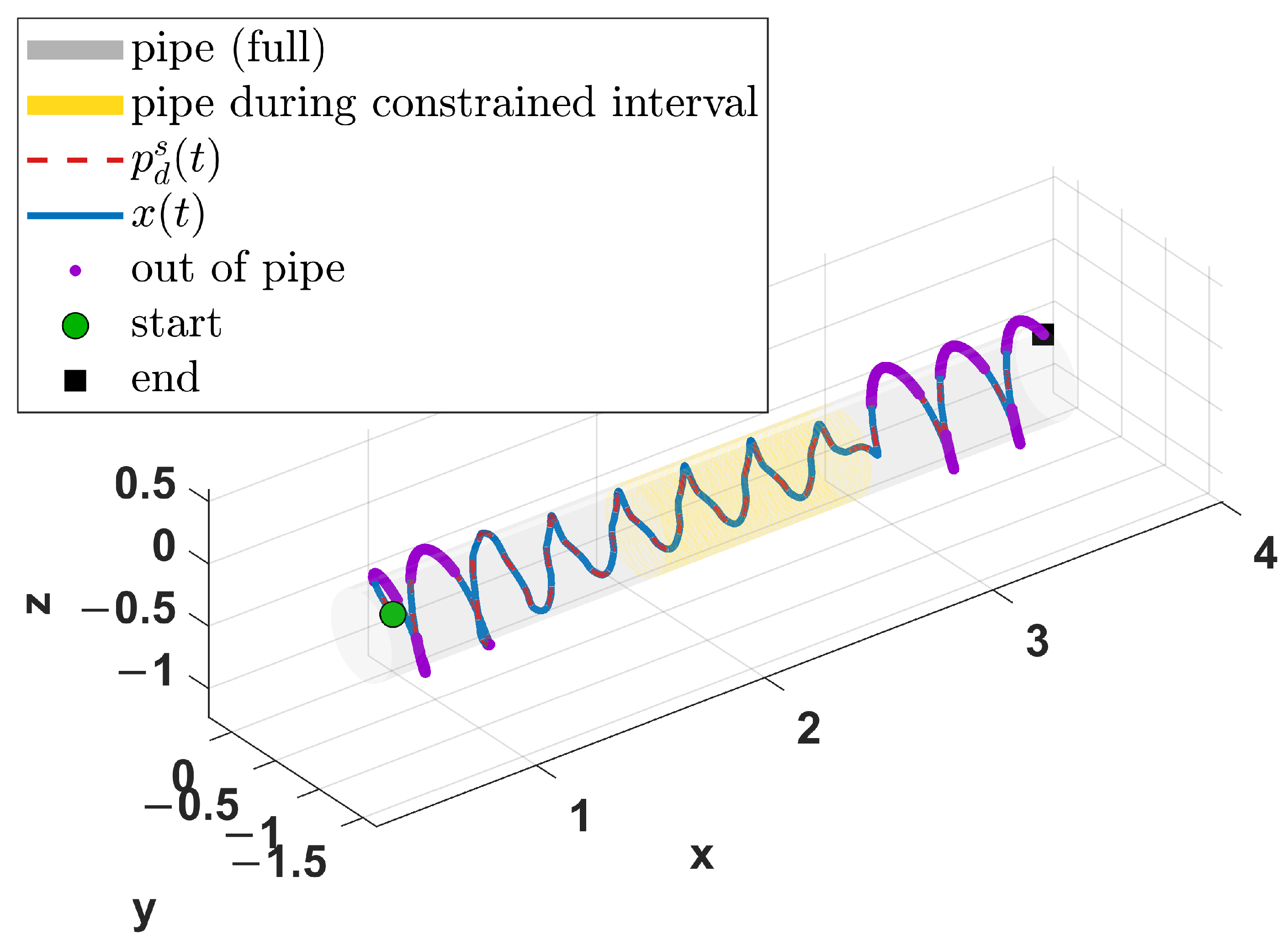
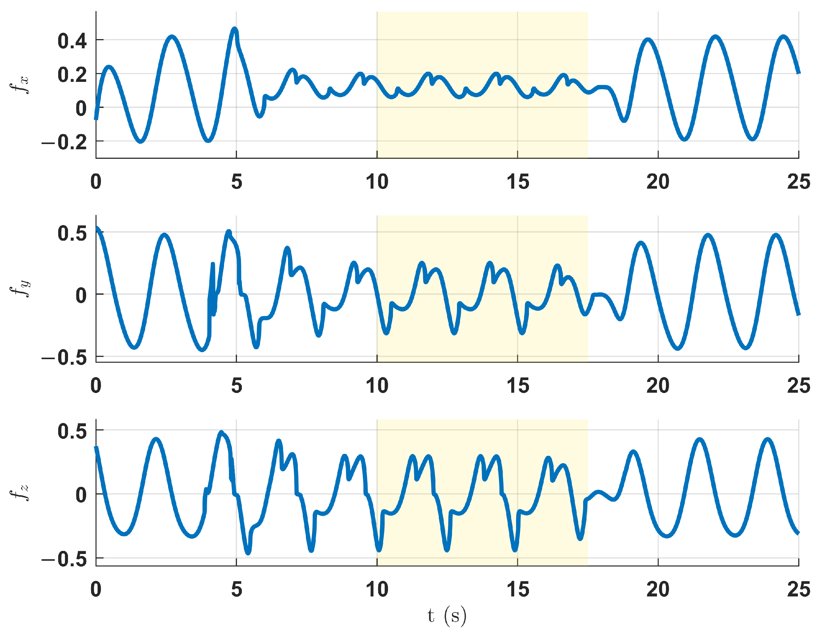
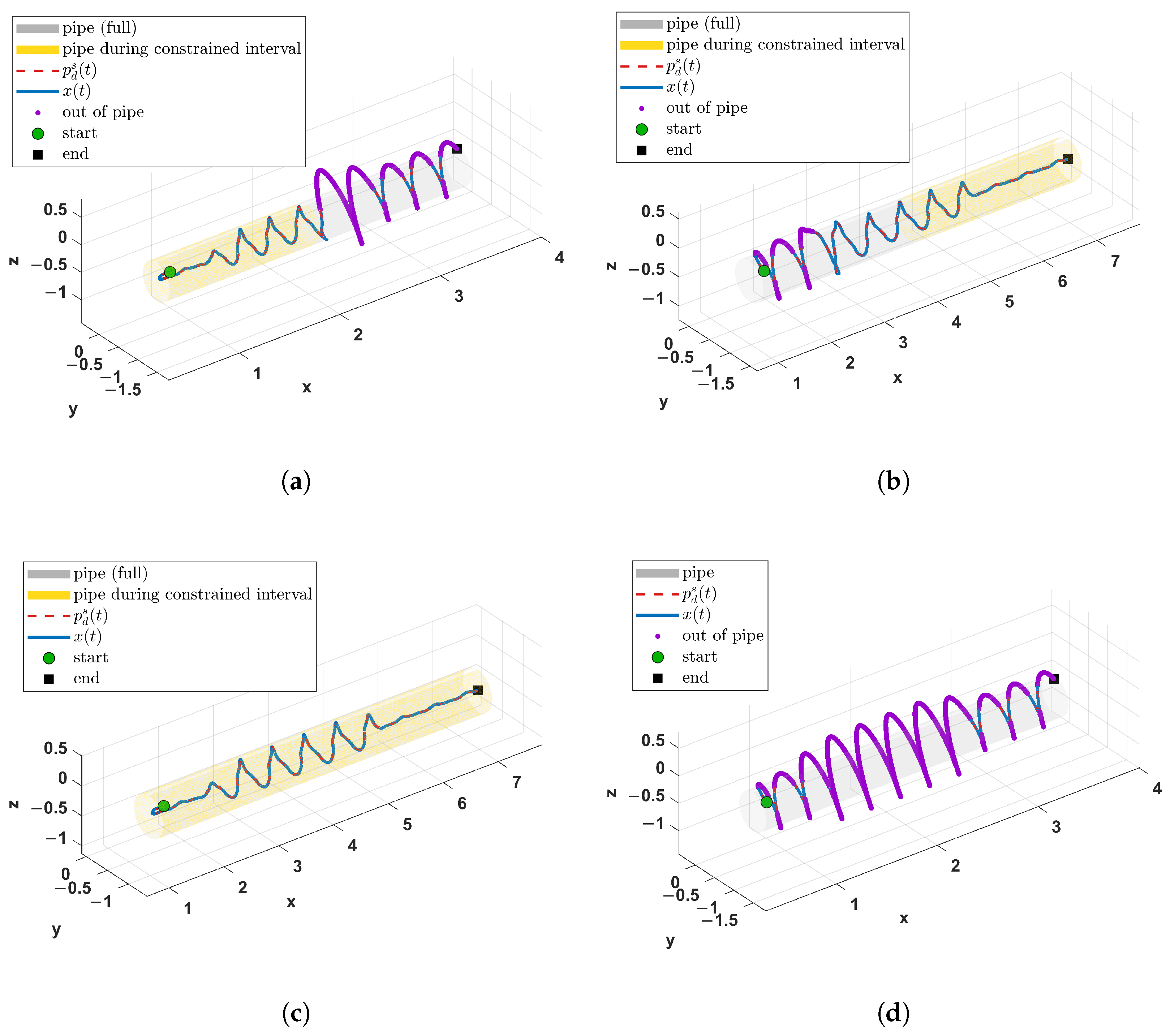
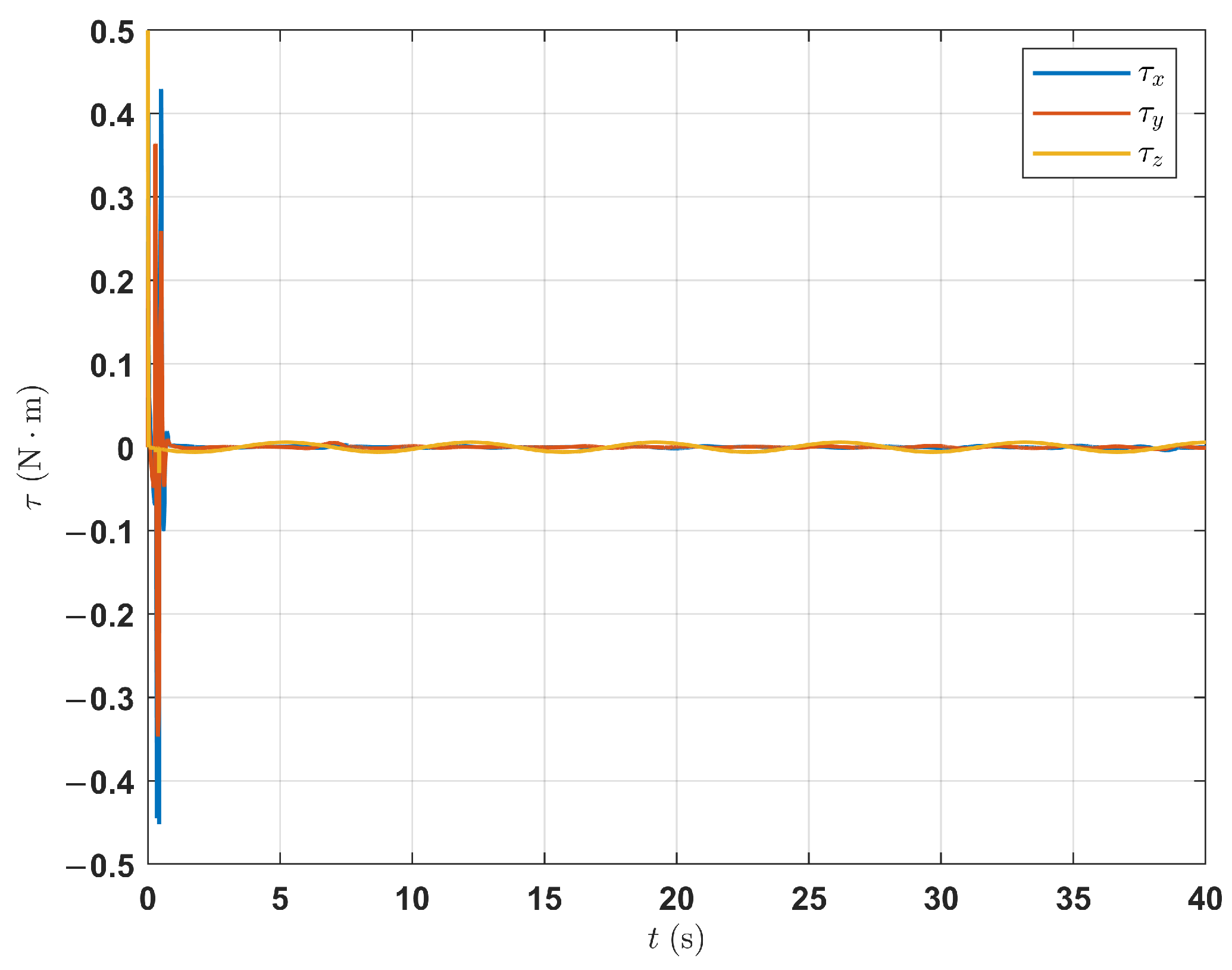
Simulations were conducted in the MATLAB R2023b environment, with results presented in Figure 5, Figure 6 and Figure 7. To demonstrate the effectiveness of the proposed UTCs mechanism, we first present the three-dimensional trajectory results of a UAV under straight-pipe constraints, as shown in Figure 5. The blue curve represents the UAV’s actual trajectory x ( t ) , the dashed line indicates the desired trajectory p d ( t ) , and the yellow area signifies the constraint activation interval. Notably, in the results depicted in Figure 5 the UTCs are not violated, ensuring L ̲ s ( t ) < x 1 s ( t ) < L ¯ s . This demonstrates that the proposed control strategy effectively ensures the system satisfies the designed state constraints. Figure 6 shows the time response of the control input, indicating that all signals remain bounded even during constraint activation, which validates the effectiveness and robustness of the proposed control strategy. Furthermore, as shown in Figure 7, the UTCs are extended to specific scenarios, demonstrating that the proposed constraint function can handle fixed-time tracking problems under various constraint scenarios, including scenario (a) initial constraints, scenario (b) delayed constraints, scenario (c) continuous constraints, and scenario (d) unconstrained. Simulation results demonstrate that the proposed adaptive constrained tracking control scheme effectively addresses position tracking under three-dimensional straight-pipe constraints. Within the constraint activation window, the obstacle function ensures the system state remains within bounds, validating the scheme’s tracking performance and robustness.
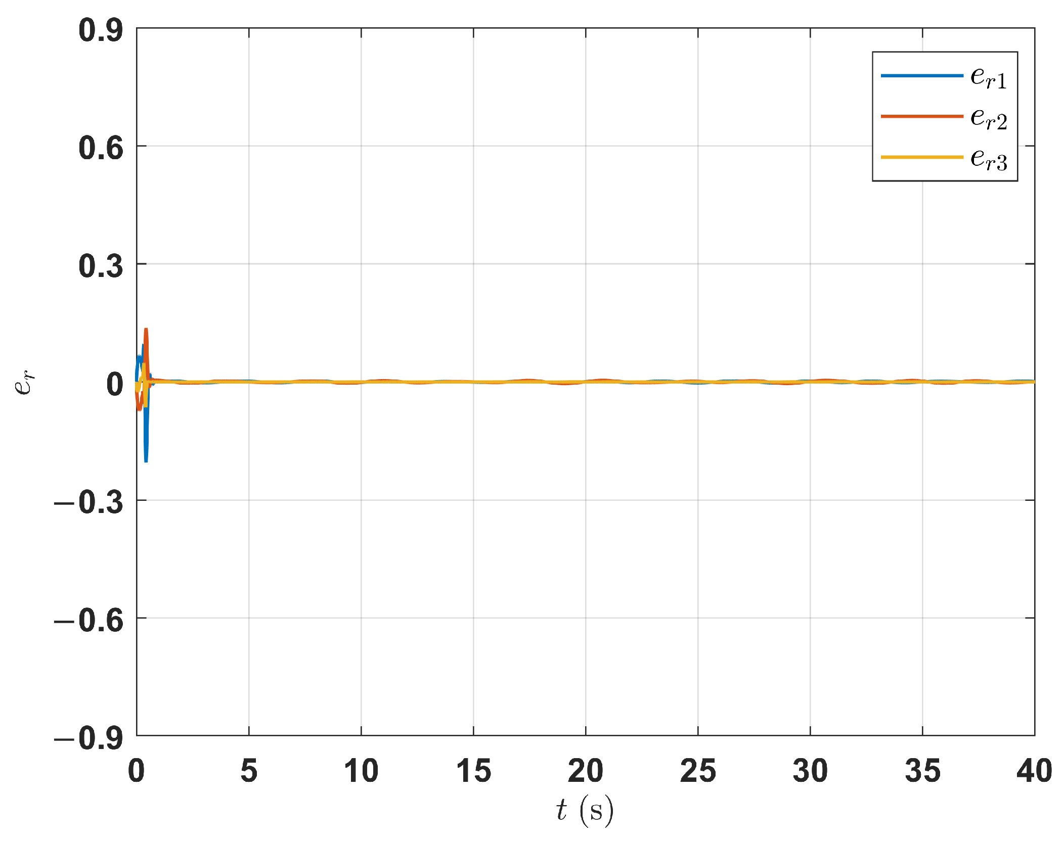
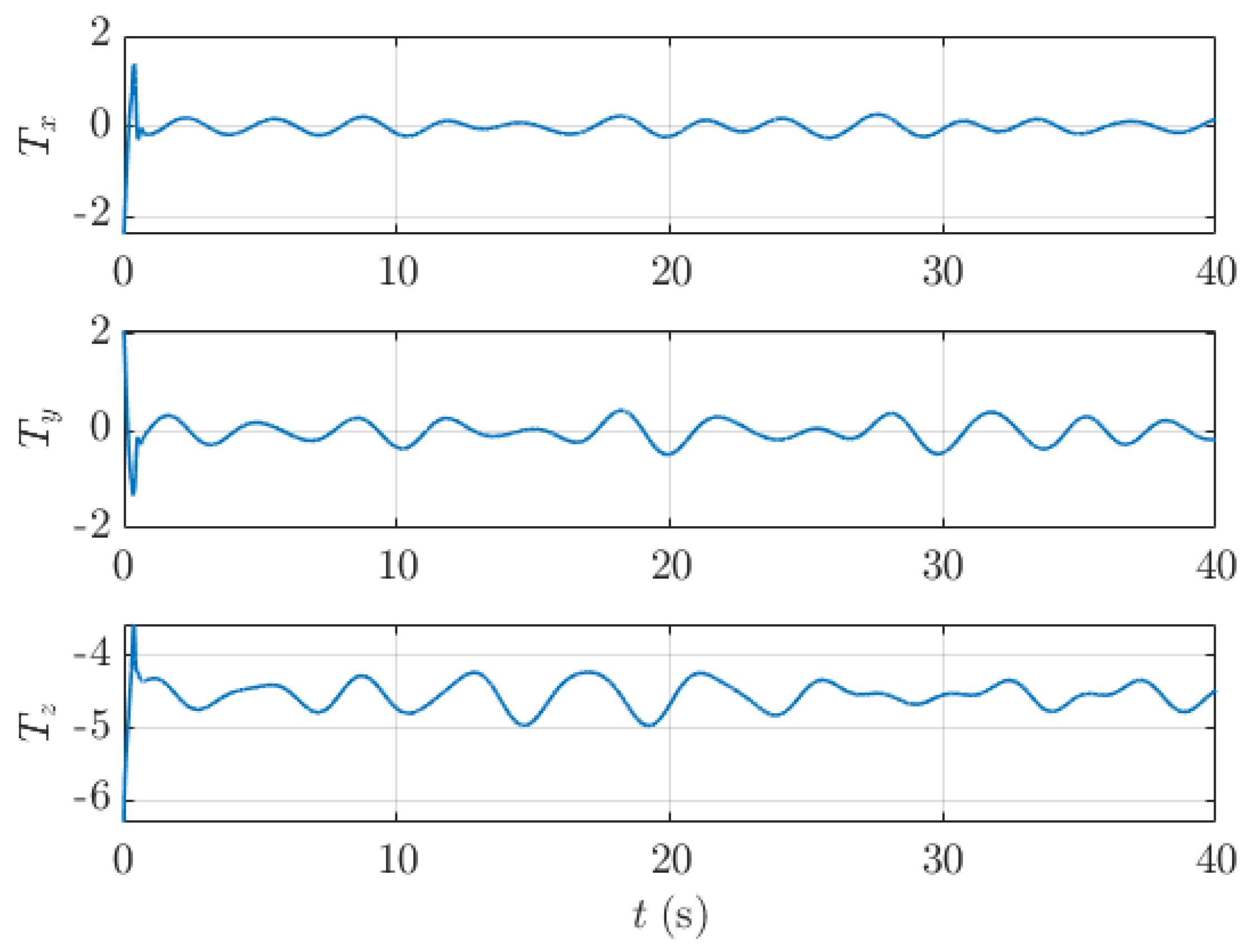
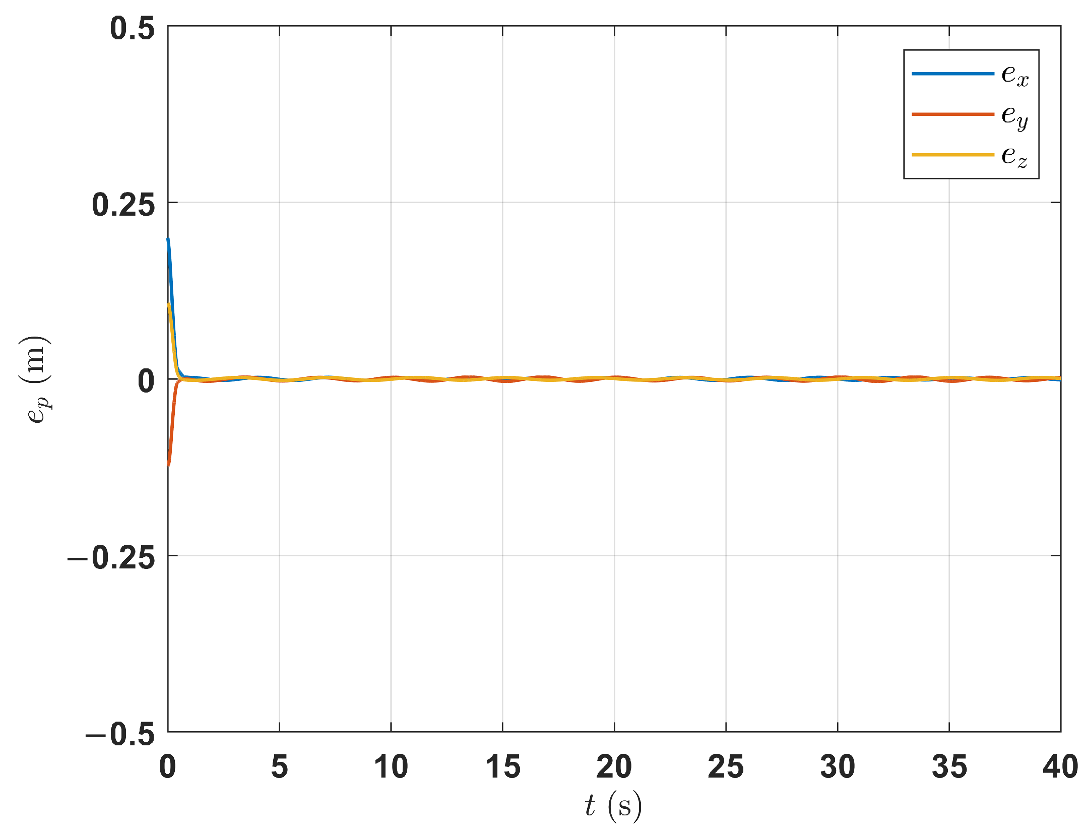
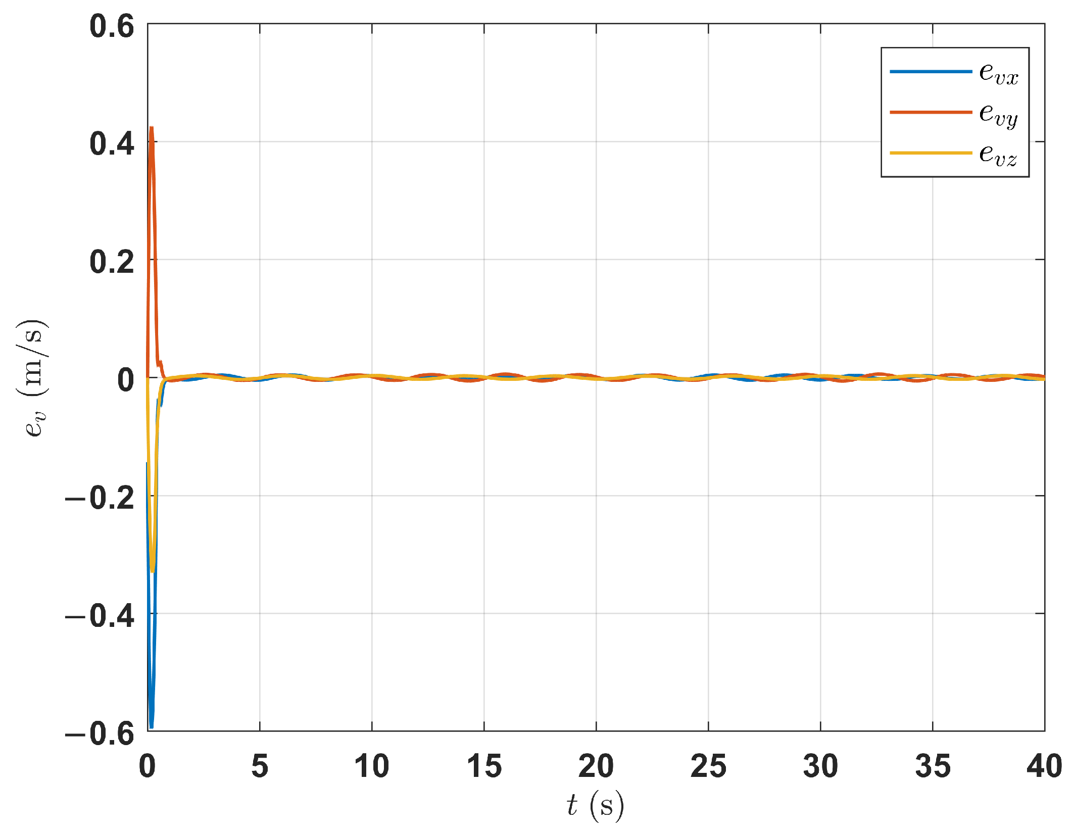
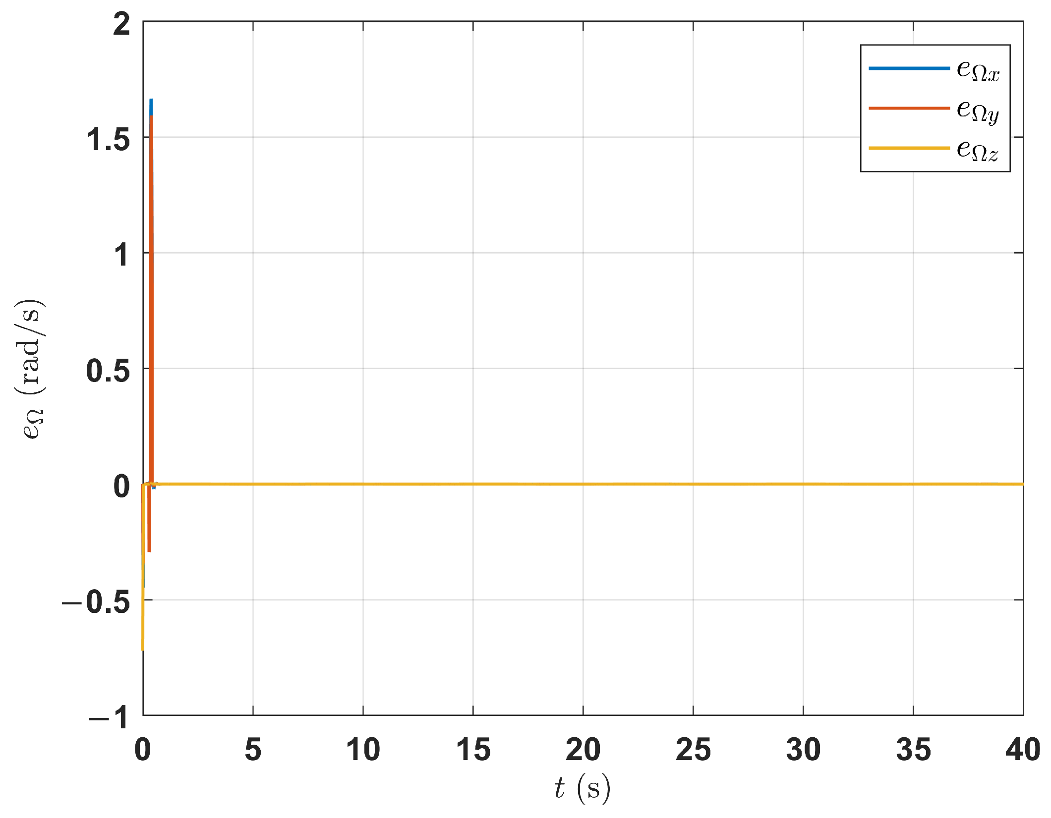
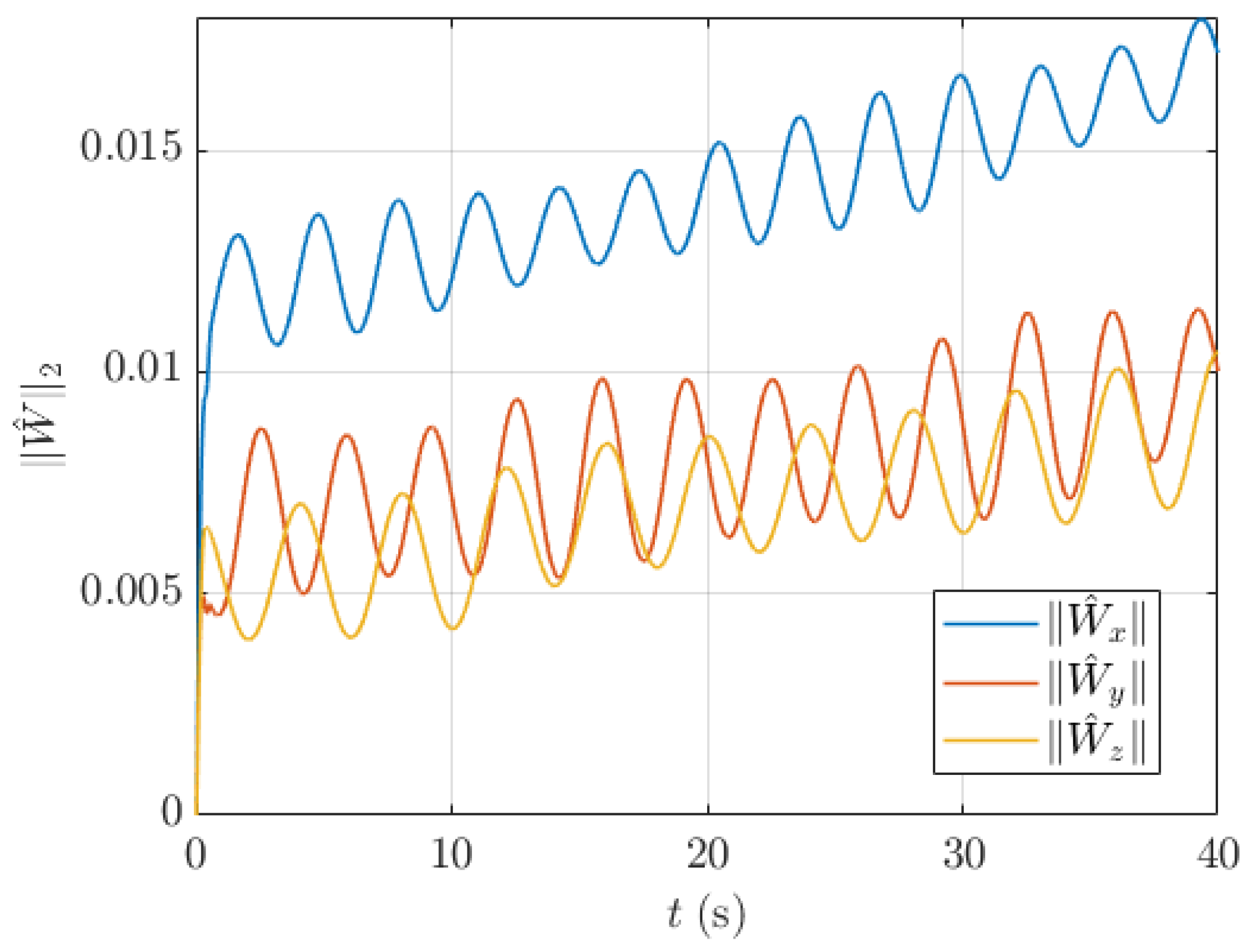
To further evaluate the overall tracking performance of the proposed controller, the simulation results are presented in Figure 8, Figure 9, Figure 10, Figure 11, Figure 12, Figure 13 and Figure 14, which demonstrate the variation in system tracking error, the approximation behavior of the neural network, the control input response, and the system state tracking performance. Figure 8, Figure 9, Figure 10 and Figure 11 illustrate the variations in tracking errors for the translational and attitude subsystems, corresponding to position tracking error z 1 , velocity tracking error z 2 , attitude error e r , and angular velocity error e Ω , respectively. According to the desired thrust vector design, the desired thrust vector control input for the translational subsystem is given by (27), which is f d = [ K 21 1 2 3 4 Θ 2 ( z 2 ) K 22 1 2 2 z 2 z 2 T z 2 + W ^ T S ( Z ) d ^ z 1 1 2 z 2 ] . As shown in Figure 8, Figure 9, Figure 10 and Figure 11, all tracking errors rapidly converge to a small neighborhood near zero after a brief transient phase and remain bounded throughout the simulation. This demonstrates that the proposed control method ensures stable tracking of the UAV’s translational and attitude dynamics systems. Furthermore, to verify the effectiveness of the proposed method in compensating for unknown disturbances, Figure 12 depicts the dynamic response of the system under uncertain conditions. The neural network weights are updated online according to the adaptive law defined in (28), which ensures the boundedness of the weights and supports an effective approximation of the unknown dynamics. To further analyze the control actions generated by the controller, Figure 13 and Figure 14 present the control input responses for thrust T and control torque τ , respectively.
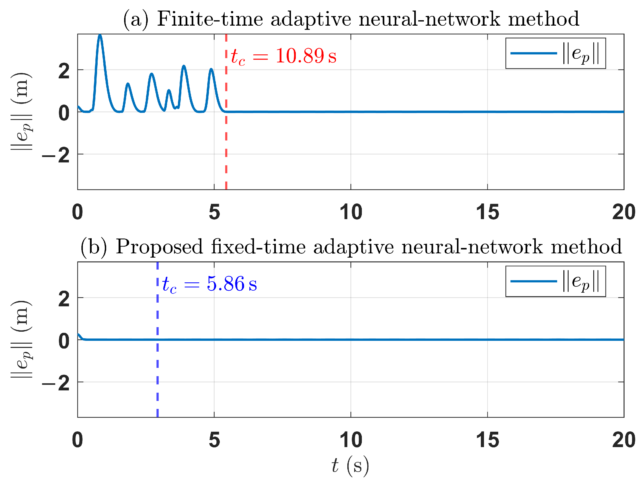
To better demonstrate the performance of the proposed method, a comparative simulation is carried out between a representative finite-time adaptive neural-network method and the proposed fixed-time adaptive neural-network method. For fairness, both methods are implemented under the same initial conditions, reference trajectory, non-harmonic disturbance, neural-network structure, and main design parameters listed in Table 1. The Euclidean norm of the position tracking error, i.e., e p , is shown in Figure 15. It can be observed that the finite-time method ensures convergence; however, the settling time is relatively longer. In contrast, the proposed method achieves faster convergence of e p , which is consistent with the theoretical analysis. These results further verify the advantage of the proposed method in terms of convergence rate and time predictability.
In summary, simulation results demonstrate that the proposed fixed-time control strategy based on adaptive neural networks achieves precise trajectory tracking while satisfying UTCs. Concurrently, the neural network effectively compensates for unknown disturbances within the system, maintaining smooth and bounded control inputs. This validates the effectiveness and robustness of the proposed control method.

5. Conclusions

This paper has investigated the fixed-time tracking control problem for an underactuated quadcopter UAV system subject to mass parameter uncertainties and UTCs. By incorporating backstepping techniques, it has proposed a neural network-based adaptive control strategy that has ensured the tracking error converges to a small region near the origin within a fixed time, while effectively avoiding singularity issues. The approximation capabilities of the neural network have been utilized to effectively compensate for uncertainties in the system dynamics. Furthermore, the controller design has incorporated a unified constraint framework with a shift function to handle more general UTCs, while also enabling flexible adaptation to different constraint scenarios without altering the adaptive structure. Finally, simulation results have validated the effectiveness of the proposed method. This work supports the advancement of UAVs systems in time-critical, safety-constrained, and dynamically evolving environments, including agile maneuvering, emergency response, and autonomous operations under transient state constraints. Future work will focus on the study and experimental validation of prescribed-time tracking control for UAVs systems in complex environments.

Author Contributions

Conceptualization, J.W. and H.L.; methodology, H.L.; software, J.W.; validation, J.W.; formal analysis, J.W.; investigation, H.L.; resources, X.Z. and Z.Q.; writing—original draft preparation, J.W.; writing—review and editing, H.L., X.Z., Y.S. and Z.Q.; supervision, H.L. and X.Z.; project administration, H.L.; funding acquisition, X.Z. and Y.S. All authors have read and agreed to the published version of the manuscript.

Funding

This research was funded by the Jiangsu Provincial Natural Science Foundation Youth Fund (Grant No. BK20251034) and the Natural Science Fundamental Research Project of Jiangsu Colleges and Universities (Grant No. 25KJB590001).

Institutional Review Board Statement

Not applicable.

Informed Consent Statement

Not applicable.

Data Availability Statement

The data presented in this study are available on request from the corresponding author.

Conflicts of Interest

The authors declare no conflicts of interest.

Appendix A. Proof of Theorem 1

Proof. 
Construct the following Lyapunov function:
V = V 1 + V 2 + V 3 + V 4 + V 5 + V 6
Substituting Equations (20), (30), (48), (50), (60) and (67) into the time derivative of V yields
V ˙ K 11 V 1 3 4 K 21 V 2 3 4 λ max 3 4 m K 31 V 3 3 4 K 41 V 4 3 4 K 12 V 1 2 K 2 V 2 2 λ max 2 m K 32 V 3 2 K 42 V 4 2 + G K r 1 V 5 3 4 K Ω 1 V 6 3 4 λ max 3 4 J K r 2 V 5 2 K Ω 2 V 6 2 λ max 2 J ,
where K 31 = min σ k 2 ( 3 / 4 ) / λ max ( 3 / 4 ) Γ k 1 , K 32 = min 4 9 κ k ( 4 / 3 ) / λ max 2 Γ k 1 , k = 1 , 2 , , n , K 41 = 2 ( 3 / 4 ) χ , K 42 = 4 9 ι ( 4 / 3 ) , G = G 1 + G 2 1 / 2 ε ¯ 2 + ϑ 1 + ϑ 2 + ϑ r + ϑ Ω + ϕ r + ϕ Ω .
By Lemmas 3 and 4, it follows readily that
μ 1 V 3 4 K 11 V 1 3 4 K 21 V 2 3 4 λ max 3 4 m K 31 V 3 3 4 K 41 V 4 3 4 K r 1 V 5 3 4 K Ω 1 V 6 3 4 λ max 3 4 J ,
μ 2 n + 5 V 2 K 12 V 1 2 K 22 V 2 2 λ max 2 m K 32 V 3 2 K 42 V 4 2 K r 2 V 5 2 K Ω 2 V 6 2 λ max 2 J
where
μ 1 = min K 11 , K 21 / λ max ( 3 / 4 ) ( m ) , K 31 , K 41 , K r 1 , K Ω 1 / λ max ( 3 / 4 ) ( J ) ,
μ 2 = min K 12 , K 22 / λ max 2 m , K 32 , K 42 , K r 2 , K Ω 2 / λ max 2 J .
Based on (A2) and (A3), (A4) can be rewritten as
V μ 1 V 3 4 μ 2 n + 5 V 2 + G
From (68) it can be seen that if V 2 G ( n + 5 ) / μ 2 then V ˙ μ 1 ( V ) ( 3 / 4 ) 0 holds. Hence V is bounded. When V 2 G ( n + 5 ) / ω μ 2 and 0 < ω < 1 , it follows that G ω μ 2 / ( n + 5 ) V 2 , and combining this with V μ 1 V 3 4 μ 2 n + 5 V 2 + G yields V ˙ μ 1 V ( 3 / 4 ) ( 1 ω ) ( μ 2 / n + 5 ) V 2 . By Lemma 5, it easily follows that V converges to the compact set V | V G ( n + 5 ) / ω μ 2 within a fixed time, with an upper bound on the convergence time given by T c o . Moreover, it is evident that 1 / 2 z 1 T z 1 V G ( n + 5 ) / ω μ 2 , z 1     2 G ( n + 5 ) / ω μ 2 = A is easily obtained, and thus it follows that z 1 converges to the compact set Ω z 1 in finite time. Similarly, z 2 , d ˜ , W ˜ , e r , e Ω also converges to the compact set Ω z 2 , Ω d ˜ , Ω W ˜ , Ω e r , Ω e Ω in finite time. Theorem 1 is proved. □

References

  1. Yogi, S.C.; Behera, L.; Nahavandi, S. Adaptive Intelligent Minimum Parameter Singularity Free Sliding Mode Controller Design for Quadrotor. IEEE Trans. Autom. Sci. Eng. 2024, 21, 1805–1823. [Google Scholar] [CrossRef] [Scilit]
  2. Roberts, A.; Tayebi, A. Adaptive Position Tracking of VTOL UAVs. IEEE Trans. Robot. 2011, 27, 129–142. [Google Scholar] [CrossRef] [Scilit]
  3. Li, K.; Ran, G.T.; Xiao, Y.Z.; Guo, Y.N.; Wu, W.R. Trajectory optimization under uncertainty: A convex optimization approach with polynomial chaos-based uncertainty quantification. Chin. J. Aeronaut. 2025, 103864. [Google Scholar] [CrossRef] [Scilit]
  4. Yin, S.; Li, C.J.; Fadda, E.; Guo, Y.N.; Ran, G.T.; Brandimarte, P. On-orbit refueling robust mission scheduling with uncertain duration for geosynchronous orbit spacecraft. Chin. J. Aeronaut. 2025, 39, 103774. [Google Scholar] [CrossRef] [Scilit]
  5. He, W.; Chen, Y.H.; Yin, Z. Adaptive Neural Network Control of an UncertainRobot with Full-State Constraints. IEEE Trans. Cybern. 2016, 46, 620–629. [Google Scholar] [CrossRef] [Scilit] [PubMed]
  6. He, W.; Ge, S.S.; Li, Y.; Chew, E.; Ng, Y.S. Neural network control of a rehabilitation robot by state and output feedback. J. Intell. Robot Syst. 2015, 80, 15–31. [Google Scholar] [CrossRef] [Scilit]
  7. Imran, I.H.; Wood, K.; Montazeri, A. Adaptive Control of Unmanned Aerial Vehicles with Varying Payload and Full Parametric Uncertainties. Electronics 2024, 13, 347. [Google Scholar] [CrossRef] [Scilit]
  8. Hu, J.H.; Xian, B.; Shao, P. Fault Tolerant Control for Unmanned Aerial Vehicle Formation Based on Distributed Nonlinear Model Predictive Control. IEEE/ASME Trans. Mechatronics 2026, 1–11. [Google Scholar] [CrossRef] [Scilit]
  9. Sun, J.R.; Li, C.J.; Ran, G.T.; Su, R.; Guo, Y.N. Two-stage cooperative trajectory planning for hypersonic glide vehicles: A bio-inspired optimization approach. Aerosp. Sci. Technol. 2026, 174, 111909. [Google Scholar] [CrossRef] [Scilit]
  10. Bianchi, A.; Borri, S.; Di Gennaro, S.; Preziuso, M. UAV trajectory control with rule-based minimum-energy reference generation. In Proceedings of the 2022 European Control Conference (ECC), London, UK, 12–15 July 2022; pp. 1497–1502. [Google Scholar]
  11. Komiyama, S.; Uchiyama, K.; Masuda, K. Combined Robust Control for Quadrotor UAV Using Model Predictive Control and Super-Twisting Algorithm. Drones 2025, 9, 576. [Google Scholar] [CrossRef] [Scilit]
  12. Wen, X.; Zou, W.C.; Xiang, Z.R. Finite-Time Consensus for High-Order Disturbed Multiagent Systems with Bounded Control Input. IEEE Syst. J. 2023, 17, 6380–6389. [Google Scholar] [CrossRef] [Scilit]
  13. Lv, Y.F.; Zhang, W.; Jian, L.; Chang, H.M. Multi-finite-time H-infinity controls of the coupled multi-driving servo systems with unknown disturbance. Eng. Appl. Artif. Intell. 2026, 171, 114276. [Google Scholar] [CrossRef] [Scilit]
  14. Stilhi, S.; Faehr, R.; Khadraoui, S.; Bettayeb, M.; Tadjine, M. Robust Finite-Time Control Using Fractional Synergetic Techniques for Robot Manipulators. Int. J. Robust Nonlinear Control 2026, 36, 4837–4856. [Google Scholar] [CrossRef] [Scilit]
  15. He, W.L.; Xu, C.R.; Han, Q.L.; Qian, F.; Lang, Z.Q. Finite-Time L2 Leader–Follower Consensus of Networked Euler–Lagrange Systems with External Disturbances. IEEE Trans. Syst. Man Cybern. Syst. 2018, 48, 1920–1928. [Google Scholar] [CrossRef] [Scilit]
  16. Liu, Y.; Li, H.Y.; Zuo, Z.Y.; Li, X.D.; Lu, R.Q. An Overview of Finite/Fixed-Time Control and Its Application in Engineering Systems. IEEE/CAA J. Autom. Sin. 2022, 9, 2106–2120. [Google Scholar] [CrossRef] [Scilit]
  17. Singh, P.; Giri, D.K.; Ghosh, A.K. Robust backstepping sliding mode aircraft attitude and altitude control based on adaptive neural network using symmetric BLF. Aerosp. Sci. Technol. 2022, 126, 107653. [Google Scholar] [CrossRef] [Scilit]
  18. Ni, J.K.; Shi, P. Adaptive Neural Network Fixed-Time Leader–Follower Consensus for Multiagent Systems with Constraints and Disturbances. IEEE Trans. Cybern. 2021, 51, 1835–1848. [Google Scholar] [CrossRef] [Scilit] [PubMed]
  19. Sui, S.; Chen, C.L.P.; Tong, S.C. A Novel Full Errors Fixed-Time Control for Constraint Nonlinear Systems. IEEE Trans. Autom. Control 2023, 68, 2568–2575. [Google Scholar] [CrossRef] [Scilit]
  20. Wang, S.B.; Sun, C.B.; Chen, Q.; He, H.R. Composite Learning Fixed-Time Control for Nonlinear Servo Systems with State Constraints and Unknown Dynamics. IEEE Trans. Syst. Man Cybern. Syst. 2025, 55, 2332–2342. [Google Scholar] [CrossRef] [Scilit]
  21. Liu, J.; Liu, J.; Wu, Y.B.; Mu, C.X.; Sun, C.Y. Aperiodically Intermittent Event-Based Fixed-Time Consensus Tracking and Its Applications. IEEE Trans. Autom. Sci. Eng. 2024, 21, 5790–5801. [Google Scholar] [CrossRef] [Scilit]
  22. Wang, H.Y.; Cui, G.Z.; Li, H.Y. Fixed-Time Adaptive Tracking Control for a Quadrotor Unmanned Aerial Vehicle with Input Saturation. Actuators 2023, 12, 130. [Google Scholar] [CrossRef] [Scilit]
  23. Gao, J.; Guo, Y.N.; Ran, G.T.; Lam, H.K.; Li, D.Y. Fast Fixed-Time-Synchronized Time-Varying Formation Tracking Control of Quadrotor UAVs Under External Disturbances. IEEE Trans. Consum. Electron. 2026, 72, 1782–1792. [Google Scholar] [CrossRef] [Scilit]
  24. Huang, J.L.; Xie, J.J.; Huang, J.; Liu, S.K. Prescribed-Time, Event-Triggered, Adaptive, Fault-Tolerant Formation Control of Heterogeneous Air–Ground Multi-Agent Systems Under Deception Attacks and Actuator Faults. Actuators 2025, 14, 575. [Google Scholar] [CrossRef] [Scilit]
  25. Pan, Y.N.; Du, P.H.; Xue, H.; Lam, H.K. Singularity-Free Fixed-Time Fuzzy Control for Robotic Systems with User-Defined Performance. IEEE Trans. Fuzzy Syst. 2021, 29, 2388–2398. [Google Scholar] [CrossRef] [Scilit]
  26. Yao, W.; Garcia de Marina, H.; Lin, B.; Cao, M. Singularity-Free Guiding Vector Field for Robot Navigation. IEEE Trans. Robot. 2021, 37, 1206–1221. [Google Scholar] [CrossRef] [Scilit]
  27. Shi, W.R.; Hou, M.Z.; Duan, G.R. A Preset-Trajectory-Based Singularity-Free Preassigned Performance Control Approach. IEEE Trans. Autom. Control 2024, 69, 6183–6190. [Google Scholar] [CrossRef] [Scilit]
  28. Fan, J.Z.; Zhao, L. Distributed finite-time adaptive consensus tracking control for multiple AUVs with state constraints. J. Frankl. Inst. 2021, 358, 9158–9177. [Google Scholar] [CrossRef] [Scilit]
  29. Liu, H.T.; Du, G.S.; Tian, X.H.; Zou, L.P. Distributed robust tracking control for multiple Euler–Lagrange systems with full-state constraints and input saturation using an event-triggered scheme. Int. J. Robust Nonlinear Control 2021, 32, 807–829. [Google Scholar] [CrossRef] [Scilit]
  30. Cao, Y.; Cao, J.F.; Song, Y.D. Practical Prescribed Time Control of Euler–Lagrange Systems with Partial/Full State Constraints: A Settling Time Regulator-Based Approach. IEEE Trans. Cybern. 2022, 52, 13096–13105. [Google Scholar] [CrossRef] [Scilit]
  31. Liu, Y.J.; Gong, M.Z.; Liu, L.; Tong, S.C.; Chen, C.L.P. Fuzzy Observer Constraint Based on Adaptive Control for Uncertain Nonlinear MIMO Systems with Time-Varying State Constraints. IEEE Trans. Cybern. 2021, 51, 1380–1389. [Google Scholar] [CrossRef] [Scilit]
  32. Kong, L.H.; Yu, X.B.; Zhang, S. Neuro-learning-based adaptive control for state-constrained strict-feedback systems with unknown control direction. ISA Trans. 2021, 112, 12–22. [Google Scholar] [CrossRef] [Scilit]
  33. He, W.; Dong, Y.T.; Sun, C.Y. Adaptive neural network control of unknown nonlinear affine systems with input deadzone and output constraint. ISA Trans. 2015, 58, 96–104. [Google Scholar] [CrossRef] [Scilit]
  34. Wang, S.M.; Huang, J. Adaptive Leader-Following Consensus for Multiple Euler–Lagrange Systems with an Uncertain Leader System. IEEE Trans. Neural Netw. Learn. Syst. 2019, 30, 2188–2196. [Google Scholar] [CrossRef] [Scilit] [PubMed]
  35. Kong, L.H.; He, W.; Dong, Y.T.; Cheng, L.; Yang, C.G.; Li, Z.J. Asymmetric bounded neural control for an uncertain robot by state feedback and output feedback. IEEE Trans. Syst. Man Cybern. Syst. 2021, 51, 1735–1746. [Google Scholar] [CrossRef] [Scilit]
  36. Wang, H.Q.; Chen, B.; Lin, C. Adaptive neural tracking control for a class of stochastic nonlinear systems. Int. J. Robust Nonlinear Control 2014, 24, 1262–1280. [Google Scholar] [CrossRef] [Scilit]
  37. Liu, M.L.; Guo, Y.N.; Ran, G.T.; Park, J.H. Fixed-Time Consensus Tracking Control for Nonlinear Multi-Agent Systems: A Dynamic Edge/Self-Triggered Approach. IEEE Trans. Circuits Syst. II Exp. Briefs 2026, 73, 73–77. [Google Scholar] [CrossRef] [Scilit]
  38. Jin, X. Adaptive Fixed-Time Control for MIMO Nonlinear Systems with Asymmetric Output Constraints Using Universal Barrier Functions. IEEE Trans. Autom. Control 2019, 64, 3046–3053. [Google Scholar] [CrossRef] [Scilit]
  39. Zuo, Z.Y.; Han, Q.L.; Ning, B.D. Fixed-Time Stability and Stabilization. In Fixed-Time Cooperative Control of Multi-Agent Systems; Springer: Singapore, 2019; pp. 19–25. [Google Scholar]
  40. Liu, Z.C.; Bechlioulis, C.P.; Huang, J.S.; Wen, C.Y. Nonlinear Dynamic Surface Control for a Class of Uncertain Systems with Novel Nonlinear Filters. IEEE Trans. Autom. Control 2025, 70, 8290–8297. [Google Scholar] [CrossRef] [Scilit]
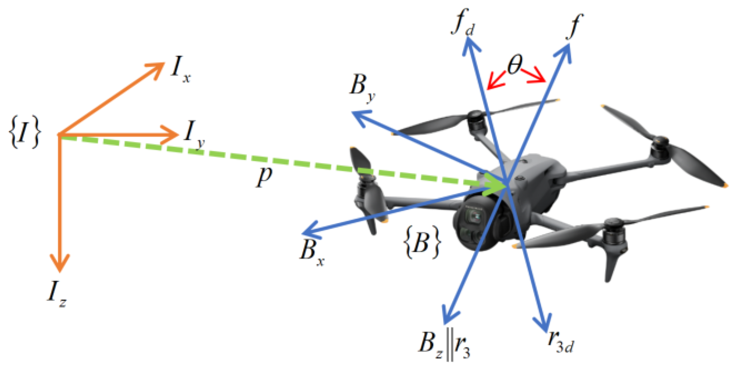
Figure 1. UAV’s framework.
Actuators 15 00270 g001
Figure 2. The trajectory of the shift function χ s ( t ) .
Actuators 15 00270 g002
Figure 3. Unified constraint framework mechanism (a) W ̲ s < β s < W ¯ s ; (b) W ̲ s χ s < z 1 s < W ¯ s χ s .
Actuators 15 00270 g003
Figure 4. Control architecture.
Actuators 15 00270 g004
Figure 5. General constraint scenarios.
Actuators 15 00270 g005
Figure 6. Control input response.
Actuators 15 00270 g006
Figure 7. (a) Initial constraints, scenario (b) delayed constraints, scenario (c) continuous constraints, and scenario (d) unconstrained.
Actuators 15 00270 g007
Figure 8. Position tracking errors.
Actuators 15 00270 g008
Figure 9. Velocity tracking errors.
Actuators 15 00270 g009
Figure 10. Attitude tracking errors.
Actuators 15 00270 g010
Figure 11. Angular velocity tracking errors.
Actuators 15 00270 g011
Figure 12. Neural network weight norms.
Actuators 15 00270 g012
Figure 13. Thrust input.
Actuators 15 00270 g013
Figure 14. Control torque inputs.
Actuators 15 00270 g014
Figure 15. Comparison of settling time based on the position tracking error norm under finite-time and fixed-time adaptive NN methods.
Actuators 15 00270 g015
Table 1. System parameters.
CategorySymbolValue
Model Parametersm0.463
g9.81
e 3 0 , 0 , 1 T
Projected Performance Parameters h r 0.40
κ h r 12
Controller gain K 11 1.8
K 12 2.2
ϖ 1 0.08
K 21 2.8
K 22 3.2
ϖ 2 0.08
K r 1 8.0
K r 2 8.0
ϖ 3 0.08
K Ω 1 4.5
K Ω 2 4.5
ϖ 4 0.08
Numerical safety T max 20
τ max 0.50
Ω max 12
Controller gain N RBF 12
Γ 0.08I
σ 0.15
b RBF 0.8
Constraint Bounds W l ( t ) [ 0.30 , 0.30 , 0.30 ] T
W u ( t ) [ 0.30 , 0.30 , 0.30 ] T
Disclaimer/Publisher’s Note: The statements, opinions and data contained in all publications are solely those of the individual author(s) and contributor(s) and not of MDPI and/or the editor(s). MDPI and/or the editor(s) disclaim responsibility for any injury to people or property resulting from any ideas, methods, instructions or products referred to in the content.