Adaptive Actor–Critic Optimal Tracking Control for a Class of High-Order Nonlinear Systems with Partially Unknown Dynamics

Abstract

Optimal tracking control for high-order partially unknown nonlinear systems poses significant challenges, particularly in deriving tractable solutions without requiring persistent excitation (PE) conditions or precise system models. This study develops an adaptive optimal tracking control law using neural network (NN)-based reinforcement learning (RL) for high-order partially unknown nonlinear systems. By designing a cost function associated with the sliding mode variable (SMV), the original tracking control problem is equivalently transformed into solving the optimal control problem related to the tracking Hamilton–Jacobi–Bellman (HJB) equation. Since the analytical solution of the HJB equation is generally intractable, we employ a policy iteration algorithm derived from the HJB equation, where both the partial derivative of the optimal tracking cost function and the optimal control law are approximated by NNs. The proposed RL framework achieves simplification through actor–critic training laws derived under the condition that a simple function is zero. Finally, both a numerical example and a single-link robotic arm application are provided to demonstrate the effectiveness and advantages of the proposed adaptive optimal tracking control method.

1. Introduction

In recent decades, optimal tracking control for nonlinear systems has remained one of the most significant research topics in control theory, with extensive applications in industrial manufacturing [1], aerospace [2], and robotics [3,4]. However, the majority of existing controller designs fail to incorporate formal optimization frameworks for performance cost functions, despite energy/time efficiency being critical in practical engineering. This study addresses this gap by developing an optimal tracking control law for partially unknown continuous-time nonlinear systems. Using an actor–critic reinforcement learning strategy derived from the HJB equation, the proposed method enables system states to achieve asymptotic tracking of the desired reference trajectory with guaranteed convergence.

Nonlinear tracking control problems can be effectively addressed through nonlinear control techniques including feedback linearization [5,6], the backstepping approach [7,8,9,10], and sliding mode control (SMC) [3,11,12,13], among others. Feedback linearization, a mature methodology in nonlinear control theory, transforms nonlinear systems into partially or fully linear equivalents through coordinated nonlinear state feedback and coordinate transformations (including dynamic compensation). This enables the application of established linear control design methods. Unlike feedback linearization, the backstepping approach provides an alternative framework for nonlinear systems unbounded by linear constraints. This methodology synthesizes feedback control laws through an iterative recursive procedure. Its principal advantage lies in preserving beneficial nonlinearities while guaranteeing asymptotic stability for regulation and tracking tasks. However, these methods are mainly applicable to strictly feedback nonlinear systems. To enhance transient response performance, SMC has garnered significant research attention. As a robust control strategy, SMC’s distinctive feature lies in its adaptive control structure switching based on state-dependent sliding surfaces. Its multiple variants have been developed, including terminal SMC [11], integral SMC [3,12], and hierarchical SMC [13]. Recent years have witnessed increasingly in-depth research on adaptive optimal control integrated with sliding mode surface (SMS). Zhang et al. addressed the problem of SMS-based adaptive optimal control for a class of switched continuous-time nonlinear systems with average dwell time by employing an actor–critic RL strategy [14]. Zhao et al. investigated the SMS-based approximate optimal control problem in the context of nonlinear multi-player Stackelberg–Nash games [15]. Furthermore, Zhang et al. studied the adaptive optimal control scheme based on a hierarchical SMS for a class of switched continuous-time nonlinear systems subject to unknown disturbances, utilizing an actor–critic NN architectures [16]. However, all of these are aimed at the problem of optimal regulation.

Designing optimal control laws for nonlinear systems typically requires solving the HJB equation. However, the inherent nonlinearity of the HJB equation makes analytical solutions challenging to derive via conventional methods. To address this, RL algorithms have been integrated into the optimal control framework, enabling feasible solutions. As a machine learning paradigm, RL allows agents to learn optimal policies through environmental interactions [17,18]. This RL-based function approximation approach has successfully enabled adaptive optimal control, emerging as a prominent methodology for complex nonlinear control in recent decades.

Current research extensively explores optimal tracking for nonlinear systems using adaptive dynamic programming (ADP) [19,20]. This method combines dynamic programming (DP) and RL. Notably, Radac et al. address the key challenge of interleaving real-time interaction with online learning in RL-based control. They propose a near real-time online RL framework for model reference tracking, which employs an extended moving window for state encoding and online backpropagation training [21]. Modares et al. proposed a novel integral RL formulation for continuous-time nonlinear systems. This approach adapts methodologies originally developed for optimal regulation problems to address optimal tracking control. Recent advancements in RL-based tracking control have demonstrated significant progress across diverse nonlinear systems [18]. Jiang et al. investigated the adaptive optimal tracking control problem for networked discrete-time linear systems by directly utilizing the data transmitted through the communication network. This problem can be addressed by solving two sub-problems: an adaptive optimal control problem and an adaptive output regulation problem. In the case of random packet loss in the network, the tracking error of the closed-loop control system has also been proven to be asymptotically stable [22]. Radac et al. proposed a novel virtual state-feedback reference feedback tuning and approximate iterative value iterative reinforcement learning method for learning the linear reference model’s output tracking control of observable systems with unknown dynamic characteristics. The approximate iterative value iterative reinforcement learning can effectively reduce the learning complexity; the virtual state-feedback reference feedback tuning can learn stable controllers even in an open-loop environment with a low exploration degree, demonstrating its superiority in tracking control learning [23]. Wen et al. developed an optimized tracking control framework employing neural network-based actor–critic reinforcement learning for a class of nonlinear dynamic systems [24]. Wang et al. subsequently proposed a novel actor–critic RL scheme to achieve optimal tracking control for unmanned surface vehicles, explicitly addressing complex unknowns including dead-zone input nonlinearities, uncertain system dynamics, and external disturbances [25]. Shi et al. proposed a robust predictive fault-tolerant control method based on signal compensation. This method established a new model for nonlinear industrial processes that contain fault factors and unknown concentrated dynamic nonlinear terms. A sub-compensator was designed to eliminate the influence of unmodeled dynamics on the control effect. This method effectively reduced the conservatism of traditional fault-tolerant control and significantly improved the tracking performance of the system [26]. Further innovations include the fuzzy integral RL-based fault-tolerant control algorithm, which integrates RL techniques with fuzzy-augmented models to handle partially unknown systems with actuator faults [27]. Specialized applications have been demonstrated, including robust online tracking control for space manipulators and the nearly optimal trajectory tracking of autonomous surface vehicles [28,29]. While the backstepping technique has been widely applied in optimal tracking control of strict-feedback nonlinear systems [30,31,32,33], the same problem for high-order canonical nonlinear systems remains largely unexplored.

Motivated by the above discussions, this paper addresses a class of canonical-form high-order nonlinear system by proposing a novel adaptive optimal tracking control scheme. The main contributions comprise three aspects. First, an adaptive optimal tracking control scheme is proposed via an SMS for high-order canonical nonlinear systems. By constructing a cost function specifically related to the SMS, the original control problem is equivalently transformed into one that seeks an optimal control strategy. The designed SMS constrains the states of the error dynamic system, thereby forcing the tracking error to converge to zero with predefined dynamics. Second, in most of the existing literature, such as [18,20,24,25], the requirement of persistent excitation is necessary for training RL optimal control with adaptive parameters. The proposed optimization method can avoid this requirement. Third, an adaptive optimal tracking law is developed using an actor–critic NN RL framework. Compared with method in [34], our method achieves higher tracking accuracy and computational efficiency with fewer conditional constraints.

The rest of this paper is organized as follows: Section 2 describes the optimal tracking control problem of a class of canonical-form high-order nonlinear system. In Section 3, we present an SMS-based adaptive optimal tracking control using actor–critic RL. Based on the Lyapunov theory, it is proven that the error signals are semi-globally uniformly ultimately bounded (SGUUB), and the tracking error can be steered into a small neighborhood of zero in Section 4. Simulations are provided to demonstrate the effectiveness of the proposed method in Section 5. Finally, the conclusion summarized in Section 6.

2. Problem Description

A canonical form nonlinear system with relative degree n is given by [35]:

$$\begin{array}{cc}\hfill & {\dot{x}}_i\left(t\right)=x_{i+1}\left(t\right),i=1,\dots ,n-1\hfill \\ \hfill & {\dot{x}}_n\left(t\right)=f\left(\overline{x}\right)+gu,\hfill \end{array}$$

(1)

where $\overline{x}\left(t\right)={\left[x_1\left(t\right),x_2\left(t\right),\dots ,x_n\left(t\right)\right]}^T\in {\mathbb{R}}^n$ is the system state vector, $u\in \mathbb{R}$ is the control input, $f\left(\overline{x}\right)\in \mathbb{R}$ is the unknown and bounded nonlinear dynamic function, and $g\in \mathbb{R}$ is the known control gain constant.

Assumption 1.

The system (1) is stabilizable, meaning there exists an admissible control policy $u\in \Psi (\Omega )$ that ensures the global stability of the closed-loop system.

Assumption 2.

The reference trajectory $y_d\left(t\right)$ and its i-th order derivatives $y_d^{\left(i\right)}\left(t\right)(i=1,\dots ,n)$ are assumed to be bounded.

Definition 1

([36]). For a nonlinear system $\dot{\zeta }=f(\zeta ,t)$, the solution $\zeta \left(t\right)\in {\mathbb{R}}^n$ is called SGUUB if for any initial state $\zeta \left(t_0\right)\in \Omega$, where Ω is a compact set, there exists constants $\sigma >0$ and $T(\sigma ,\zeta \left(t_0\right))>0$ such that $\parallel \zeta \left(t\right)\parallel ⩽\sigma$ for all $t\ge t_0+T(\sigma ,\zeta \left(t_0\right))$.

The control objective of this paper is to design an optimized tracking controller for partially unknown nonlinear dynamic system (1) using an NN-based actor–critic RL strategy. The proposed control law not only ensures all closed-loop error signals are SGUUB, but also guarantees that the output state $x_1\left(t\right)$ and its derivative signals rapidly track the reference trajectory $y_d\left(t\right)$ and its corresponding derivatives, respectively.

3. Optimal Tracking Control Design

3.1. Tracking HJB Equation

The tracking errors are defined as $z_1\left(t\right)=x_1\left(t\right)-y_d\left(t\right),z_2\left(t\right)=x_2\left(t\right)-{\dot{y}}_d\left(t\right),\dots ,$ and $z_n\left(t\right)=x_n\left(t\right)-y_d^{(n-1)}\left(t\right)$. Based on the dynamic model (1) and the above tracking error definitions, the error dynamical system is derived as follows:

$$\begin{array}{cc}\hfill & {\dot{z}}_i\left(t\right)=z_{i+1}\left(t\right),i=1,\dots ,n-1\hfill \\ \hfill & {\dot{z}}_n\left(t\right)=f(\overline{z},{\overline{y}}_d)+gu-y_d^{\left(n\right)}\left(t\right)\hfill \end{array}$$

(2)

where $\overline{z}={[z_1\left(t\right),z_2\left(t\right),\dots ,z_n\left(t\right)]}^T\in {\mathbb{R}}^n$, and ${\overline{y}}_d={[y_d\left(t\right),{\dot{y}}_d\left(t\right),\dots ,y_d^{(n-1)}\left(t\right)]}^T\in {\mathbb{R}}^n$.

Based on the tracking errors, the sliding mode variable [37] is constructed as

$$s\left(t\right)=K_0^T\overline{z}\left(t\right)=k_1{z}_1\left(t\right)+\dots +k_{n-1}{z}_{n-1}\left(t\right)+z_n\left(t\right),$$

(3)

where $s\left(t\right)\in \mathbb{R}$, $K_0={[k_1,\dots ,k_{n-1},1]}^T\in {\mathbb{R}}^n$, and $k_j>0(j=1,\dots ,n-1)$ are design parameters.

Taking the time derivative of $s\left(t\right)$ along the error dynamical system (2) yields

$$\begin{array}{cc}\hfill \dot{s}\left(t\right)& =K_1^T\overline{z}\left(t\right)+f(\overline{z},{\overline{y}}_d)+gu-y_d^{\left(n\right)}\left(t\right)=k_1{z}_2\left(t\right)+\dots +k_{n-1}{z}_n\left(t\right)\hfill \\ \hfill & +f(\overline{z},{\overline{y}}_d)+gu-y_d^{\left(n\right)}\left(t\right),\hfill \end{array}$$

(4)

where $K_1={[0,k_1,\dots ,k_{n-1}]}^T\in {\mathbb{R}}^n$.

The design parameters $k_j$ are chosen such that the polynomial ${\rho }^{n-1}+k_{n-1}{\rho }^{n-2}+\dots +k_2\rho +k_1$ is Hurwitz, i.e., all its roots lie in the open left-half plane. Note that when the tracking errors $z_1\left(t\right),\dots ,z_n\left(t\right)$ are constrained to the SMS $s\left(t\right)=0$, they will converge to a small neighborhood of zero.

Define an infinite-horizon cost function with respect to the SMS s as follows:

$$V\left(s\right)={\int }_t^{\infty }r(s\left(\tau \right),u\left(s\right))d\tau ,$$

(5)

where $r(s,u)=s^2+u^2$ denotes the utility function.

Definition 2.

For the error dynamical system (2), the control policy $u\left(s\right)$ is defined as admissible with respect to $V\left(s\right)$ on the compact set Ω, denoted by $u\left(s\right)\in \Psi (\Omega )$; if $u\left(s\right)$ is continuous, $u\left(0\right)=0$, $u\left(s\right)$ can stabilize (2) on Ω and $V\left(s\right)$ is finite for $\forall s\in \Omega$.

The optimal control objective for the error dynamical system (2) is to find an admissible control law that minimizes the cost function (5) over an infinite horizon, thus achieving the desired control task. Accordingly, the optimal cost function is defined as

$$\begin{array}{cc}\hfill V^{*}\left(s\right)& =\underset{u\in \Psi (\Omega )}{min}\left({\int }_t^{\infty }r(s\left(\tau \right),u\left(s\right))d\tau \right)={\int }_t^{\infty }r(s\left(\tau \right),u^{*}\left(s\right))d\tau ,\hfill \end{array}$$

(6)

where $V^{*}\left(s\right)$ and $u^{*}\left(s\right)$ denote the optimal cost function and optimal control law, respectively, and $\Psi (\Omega )$ represents the set of admissible controls over the domain $\Omega$.

By calculating the time derivative of the cost function (6) along the sliding mode dynamic (4) and applying the optimality condition, the following HJB equation is derived:

$$\begin{array}{cc}\hfill H(s,u^{*},\nabla V^{*}\left(s\right))& =r(s,u^{*})+\nabla V^{*}\left(s\right)\dot{s}\hfill \\ & =s^2+u^{*2}+\nabla V^{*}\left(s\right)(K_1^T\overline{z}\left(t\right)+f(\overline{z},{\overline{y}}_d)+g{u}^{*}-y_d^{\left(n\right)}\left(t\right))\hfill \\ & =0\hfill \end{array}$$

(7)

where $\nabla V^{*}\left(s\right)=\partial V^{*}\left(s\right)/\partial s$ denotes the partial derivative of $V^{*}\left(s\right)$ with respect to s.

Assuming the solution of (7) exists and is unique, the optimal control $u^{*}$ can be obtained by applying the stationarity condition ${\displaystyle \frac{\partial H(s,u^{*},\nabla V^{*}\left(s\right)}{\partial u^{*}}}=0$ as

$$u^{*}=-{\displaystyle \frac{g}{2}}\nabla V^{*}\left(s\right).$$

(8)

Substituting (8) into (7) yields

$$\begin{array}{c}\hfill s^2-{\displaystyle \frac{g^2}{4}}{\left(\nabla V^{*}\left(s\right)\right)}^2+\nabla V^{*}\left(s\right)\left(K_1^T\overline{z}\left(t\right)+f(\overline{z},{\overline{y}}_d)-y_d^{\left(n\right)}\left(t\right)\right)=0.\end{array}$$

(9)

The partial derivative $\nabla V^{*}\left(s\right)$ can be obtained by solving the HJB Equation (9). The optimal control protocol can then be derived by combining the result with (8). However, solving (9) analytically is difficult due to the inherent system nonlinearity. Furthermore, the lack of complete knowledge about the system dynamics $f(\overline{z},{\overline{y}}_d)$ further complicates the solution of (9). To overcome these challenges, this paper employs a reinforcement learning method with an actor–critic architecture.

3.2. NNs Approximation in Actor–Critic RL

To achieve the optimal tracking control, the term $\nabla V^{*}\left(s\right)$ in (9) is decomposed as

$$\nabla V^{*}\left(s\right)=2{\gamma }_{u}s\left(t\right)+{\displaystyle \frac{2}{g^2}}{K}_1^T\overline{z}\left(t\right)+{\displaystyle \frac{1}{g^2}}{V}^0(s,\overline{z}),$$

(10)

where ${\gamma }_u>0$ is the designed parameter and ${\displaystyle \frac{1}{g^2}}{V}^0(s,\overline{z})=-2{\gamma }_{u}s\left(t\right)-{\displaystyle \frac{2}{g^2}}{K}_1^T\overline{z}\left(t\right)+\nabla V^{*}\left(s\right)$ is the unknown function in this dual architecture.

Remark 1.

In (10), the terms $2{\gamma }_{u}s\left(t\right)$ and ${\displaystyle \frac{2}{g^2}}{K}_1^T\overline{z}\left(t\right)$ are designed to ensure the boundedness and stability of the system signals.

According to the Weierstrass approximation theorem [38], the continuous function $V^0(s,\overline{z})$ can be approximated by the weighted sum of basis functions. Given the relationship $s\left(t\right)=K_0^T\overline{z}\left(t\right)$ between s and $\overline{z}$, the approximation takes the form as

$$V^0(s,\overline{z})=W^{*T}\Phi \left(\overline{z}\right)+\epsilon \left(\overline{z}\right),$$

(11)

where $W^{*}=[w_1,w_2,\dots ,w_N]\in {\mathbb{R}}^N$ is the ideal weight vector and bounded by a positive constant $\overline{W}$ such that $\parallel W^{*}\parallel \le \overline{W}$. Moreover, $\Phi =[{\varphi }_1,{\varphi }_2,\dots ,{\varphi }_N]\in {\mathbb{R}}^N$ and $\epsilon \left(\overline{z}\right)\in \mathbb{R}$ are, respectively, the activation function vector and the approximation error. With the number of neurons in the hidden layer $N\to \infty$, the NN approximation error $\epsilon \left(\overline{z}\right)\to 0$.

Putting (11) into (10) yields

$$\nabla V^{*}\left(s\right)=2{\gamma }_{u}s\left(t\right)+{\displaystyle \frac{2}{g^2}}{K}_1^T\overline{z}\left(t\right)+{\displaystyle \frac{1}{g^2}}{W}^{*T}\Phi \left(\overline{z}\right)+{\displaystyle \frac{1}{g^2}}\epsilon \left(\overline{z}\right).$$

(12)

Since the ideal weight vector $W^{*}$ is unknown, (12) is approximated by a critic NN as

$$\nabla {\widehat{V}}^{*}\left(s\right)=2{\gamma }_{u}s\left(t\right)+{\displaystyle \frac{2}{g^2}}{K}_1^T\overline{z}\left(t\right)+{\displaystyle \frac{1}{g^2}}{\widehat{W}}_c^T\Phi \left(\overline{z}\right),$$

(13)

where ${\widehat{W}}_c$ denotes the current estimate of $W^{*}$. The weight estimation error is then defined as ${\tilde{W}}_c={\widehat{W}}_c-W^{*}$.

According to (8) and (13), the optimal control to the system is approximated by an additional actor NN as

$${\widehat{u}}^{*}=-g{\gamma }_{u}s\left(t\right)-{\displaystyle \frac{1}{g}}{K}_1^T\overline{z}\left(t\right)-{\displaystyle \frac{1}{2g}}{\widehat{W}}_a^T\Phi \left(\overline{z}\right),$$

(14)

where ${\widehat{W}}_a$ is the current estimate of $W^{*}$. The actor NN weight estimation error is defined as ${\tilde{W}}_a={\widehat{W}}_a-W^{*}$.

The critic and actor adaptive training laws are designed as

$$\begin{array}{c}\hfill {\dot{\widehat{W}}}_c\left(t\right)=-{\gamma }_c\left(\Phi \left(\overline{z}\right){\Phi }^T\left(\overline{z}\right)+\sigma I_m\right){\widehat{W}}_c\left(t\right),\end{array}$$

(15)

$${\dot{\widehat{W}}}_a\left(t\right)=-\left(\Phi \left(\overline{z}\right){\Phi }^T\left(\overline{z}\right)+\sigma I_m\right)\left[{\gamma }_a\left({\widehat{W}}_a\left(t\right)-{\widehat{W}}_c\left(t\right)\right)-{\gamma }_c{\widehat{W}}_c\left(t\right)\right],$$

(16)

where ${\gamma }_c>0$ and ${\gamma }_a>0$ are the learning rates for the critic and actor networks, respectively. Here, $\sigma >0$ is a regularization parameter, and $I_m$ denotes the $m\times m$ identity matrix.

Inserting both (13) and (14) into (7), the approximated HJB equation yields

$$\begin{array}{cc}\hfill \widehat{H}(s,{\widehat{u}}^{*},\nabla {\widehat{V}}^{*}\left(s\right))& =s^2+g^2{\left(-{\gamma }_{u}s\left(t\right)-{\displaystyle \frac{1}{g^2}}{K}_1^T\overline{z}\left(t\right)-{\displaystyle \frac{1}{2g^2}}{\widehat{W}}_a^T\Phi \left(\overline{z}\right)\right)}^2\hfill \\ & +\left(2{\gamma }_{u}s\left(t\right)+{\displaystyle \frac{2}{g^2}}{K}_1^T\overline{z}\left(t\right)+{\displaystyle \frac{1}{g^2}}{\widehat{W}}_c^T\left(t\right)\Phi \left(\overline{z}\right)\right)\hfill \\ & \times \left(-g^2{\gamma }_{u}s\left(t\right)-{\displaystyle \frac{1}{2}}{\widehat{W}}_a^T\Phi \left(\overline{z}\right)+f(\overline{z},{\overline{y}}_d)-y_d^{\left(n\right)}\left(t\right)\right).\hfill \end{array}$$

(17)

The Bellman residual error E is introduced, with the following expression:

$$\begin{array}{cc}\hfill E& =\widehat{H}(s,{\widehat{u}}^{*},\nabla {\widehat{V}}^{*}\left(s\right))-H(s,u^{*},\nabla V^{*}\left(s\right))\hfill \\ \hfill & =\widehat{H}(s,{\widehat{u}}^{*},\nabla {\widehat{V}}^{*}\left(s\right))\hfill \end{array}$$

(18)

According to the previous analysis and the optimal control theory, the approximate optimized control ${\widehat{u}}^{*}$ should ensure $E\to 0$. If the condition $E=0$ is met and has a unique solution, it is equivalent to

$$\begin{array}{c}\hfill {\displaystyle \frac{\partial \widehat{H}(s,{\widehat{u}}^{*},\nabla {\widehat{V}}^{*}\left(s\right))}{\partial {\widehat{W}}_a}}={\displaystyle \frac{1}{2g^2}}\Phi \left(\overline{z}\right){\Phi }^T\left(\overline{z}\right)\left({\widehat{W}}_a\left(t\right)-{\widehat{W}}_c\left(t\right)\right)=0.\end{array}$$

(19)

To make (19) hold, construct the following function $\Gamma \left(t\right)$ such that

$$\begin{array}{c}\hfill \Gamma \left(t\right)={\left({\widehat{W}}_a\left(t\right)-{\widehat{W}}_c\left(t\right)\right)}^T\left({\widehat{W}}_a\left(t\right)-{\widehat{W}}_c\left(t\right)\right).\end{array}$$

(20)

Obviously, $\Gamma \left(t\right)=0$ ensures that (19) holds. When the weight vectors of both networks are trained to satisfy ${\widehat{W}}_a\left(t\right)={\widehat{W}}_c\left(t\right)$, Equations (13) and (14) fulfill the relation (8), and the control action approaches the optimal solution.

Theorem 1.

Under the adaptive laws given by (15) and (16), the function $\Gamma \left(t\right)$ converges to zero asymptotically.

Proof. 

The partial derivatives of $\Gamma \left(t\right)$ with respect to the weight estimates are

$${\displaystyle \frac{\partial \Gamma \left(t\right)}{\partial {\widehat{W}}_a\left(t\right)}}=-{\displaystyle \frac{\partial \Gamma \left(t\right)}{\partial {\widehat{W}}_c\left(t\right)}}=2\left({\widehat{W}}_a\left(t\right)-{\widehat{W}}_c\left(t\right)\right).$$

(21)

The time derivative of $\Gamma \left(t\right)$ along the trajectories of the system is

$$\begin{array}{cc}\hfill \dot{\Gamma }\left(t\right)& ={\displaystyle \frac{\partial \Gamma \left(t\right)}{\partial {\widehat{W}}_a\left(t\right)}}{\dot{\widehat{W}}}_a\left(t\right)+{\displaystyle \frac{\partial \Gamma \left(t\right)}{\partial {\widehat{W}}_c\left(t\right)}}{\dot{\widehat{W}}}_c\left(t\right)={\displaystyle \frac{\partial \Gamma \left(t\right)}{\partial {\widehat{W}}_a\left(t\right)}}\left({\dot{\widehat{W}}}_a\left(t\right)-{\dot{\widehat{W}}}_c\left(t\right)\right).\hfill \end{array}$$

(22)

Substituting the adaptive laws (15) and (16) into (22) yields

$$\begin{array}{cc}\hfill \dot{\Gamma }\left(t\right)& =2{\left({\widehat{W}}_a-{\widehat{W}}_c\right)}^T\left[-{\gamma }_a\left(\Phi \left(\overline{z}\right){\Phi }^T\left(\overline{z}\right)+\sigma I_m\right)\left({\widehat{W}}_a-{\widehat{W}}_c\right)\right]\hfill \\ \hfill & =-2{\gamma }_a{\left({\widehat{W}}_a-{\widehat{W}}_c\right)}^T\left(\Phi \left(\overline{z}\right){\Phi }^T\left(\overline{z}\right)+\sigma I_m\right)\left({\widehat{W}}_a-{\widehat{W}}_c\right).\hfill \end{array}$$

(23)

Noting that $\Gamma \left(t\right)=\parallel {\widehat{W}}_a-{\widehat{W}}_c{\parallel }^2$, the expression in (23) can be rewritten as a function of $\Gamma \left(t\right)$ itself. Since the matrix $\left(\Phi \left(\overline{z}\right){\Phi }^T\left(\overline{z}\right)+\sigma I_m\right)$ is positive definite, it follows that

$$\begin{array}{cc}\hfill \dot{\Gamma }\left(t\right)& =-2{\gamma }_a{\left({\widehat{W}}_a-{\widehat{W}}_c\right)}^T\left(\Phi \left(\overline{z}\right){\Phi }^T\left(\overline{z}\right)+\sigma I_m\right)\left({\widehat{W}}_a-{\widehat{W}}_c\right)\hfill \\ \hfill & \le -2{\gamma }_a{\lambda }_{min}{\parallel {\widehat{W}}_a-{\widehat{W}}_c\parallel }^2=-2{\gamma }_a{\lambda }_{min}\Gamma \left(t\right),\hfill \end{array}$$

(24)

where ${\lambda }_{min}>0$ is the minimum eigenvalue of the positive definite matrix $\left(\Phi \left(\overline{z}\right){\Phi }^T\left(\overline{z}\right)+\sigma I_m\right)$.

This inequality, $\dot{\Gamma }\left(t\right)\le -2{\gamma }_a{\lambda }_{min}\Gamma \left(t\right)$, implies that $\Gamma \left(t\right)$ converges to zero exponentially. □

Remark 2.

The critic NN in (14) may be used to determine the actor without using another NN for the actor. However, to obtain the form of (19) and to facilitate the derivation of weight update laws and subsequent stability analysis, separate NNs are necessary for the actor and critic.

Remark 3.

This paper presents an online reinforcement learning framework based on an actor–critic architecture. The actor and critic networks are employed to approximate the optimal control law and the value function gradient, respectively. Critically, the update laws for the network weights are derived from the convergence condition of a constructed scalar function $\Gamma \left(t\right)$ to zero, rather than from the minimization of the Bellman residual error. This constitutes a key methodological departure. Conventional adaptive dynamic programming methods typically design update laws by minimizing the squared Bellman residual. However, solving this nonlinear equation online is computationally complex. The proposed approach, by leveraging the simple convergence condition of $\Gamma \left(t\right)$, circumvents this complexity, thereby significantly reducing the online computational burden of the control design.

Remark 4.

As demonstrated in this subsection, the proposed RL approach not only features a simple structure but also eliminates the need for explicit knowledge of the system dynamic $f(\overline{z},{\overline{y}}_d)$ when solving the optimal control problem.

4. Main Results

Lemma 1

([39]). $X\left(t\right)\in \mathbb{R}$ is a positive continuous function and has the bounded initial value $X\left(0\right)$. If the inequality $\dot{X}\left(t\right)⩽-\alpha X\left(t\right)+\beta$ holds, where $\alpha >0$ and $\beta >0$ are constants, then

$$X\left(t\right)⩽e^{-\alpha t}X\left(0\right)+{\displaystyle \frac{\beta }{\alpha }}(1-e^{-\alpha t}).$$

(25)

Theorem 2.

Consider the partially unknown nonlinear system (1) under Assumptions 1 and 2, with a bounded initial state. The optimal control law is derived from the actor–critic RL framework, where the critic and actor are updated according to (13) and (14), using the learning rules given in (15) and (16), respectively. If the parameters satisfy ${\gamma }_u>{\displaystyle \frac{1}{2}}+{\displaystyle \frac{1}{g^2}}$, ${\gamma }_c>{\displaystyle \frac{{\gamma }_a}{2}}$ and ${\gamma }_a>1$, then the tracking error vector $\overline{z}\left(t\right)$ and the weight estimation errors $\tilde{W}c\left(t\right)$ and $\tilde{W}a\left(t\right)$ are SGUUB. Moreover, the tracking errors converge to an arbitrarily small neighborhood of zero.

Proof. 

Choose the Lyapunov candidate function as

$$L\left(t\right)={\displaystyle \frac{1}{2}}{s}^2+{\displaystyle \frac{1}{2}}{\tilde{W}}_c^T\left(t\right){\tilde{W}}_c\left(t\right)+{\displaystyle \frac{1}{2}}{\tilde{W}}_a^T\left(t\right){\tilde{W}}_a\left(t\right).$$

(26)

Calculating the time derivative (26) along (4), (15) and (16) yields

$$\begin{array}{cc}\hfill \dot{L}\left(t\right)& =s\left(-g^2{\gamma }_{u}s-{\displaystyle \frac{1}{2}}{\widehat{W}}_a^T\left(t\right)\Phi \left(\overline{z}\right)+f(\overline{z},{\overline{y}}_d)-y_d^{\left(n\right)}\left(t\right)\right)-{\gamma }_c{\tilde{W}}_c^T\left(t\right)(\Phi \left(\overline{z}\right){\Phi }^T\left(\overline{z}\right)\hfill \\ & +\sigma I_m){\widehat{W}}_c\left(t\right)-{\gamma }_a{\tilde{W}}_a^T\left(t\right)\left(\Phi \left(\overline{z}\right){\Phi }^T\left(\overline{z}\right)+\sigma I_m\right)\left({\widehat{W}}_a\left(t\right)-{\widehat{W}}_c\left(t\right)\right)\hfill \\ & +{\gamma }_c{\tilde{W}}_a^T\left(t\right)\left(\Phi \left(\overline{z}\right){\Phi }^T\left(\overline{z}\right)+\sigma I_m\right){\widehat{W}}_c\left(t\right).\hfill \end{array}$$

(27)

It follows from ${\tilde{W}}_c={\widehat{W}}_c-W^{*}$ and ${\tilde{W}}_a={\widehat{W}}_a-W^{*}$ that

$${\widehat{W}}_a^T\Phi \left(\overline{z}\right)={\tilde{W}}_a^T\Phi \left(\overline{z}\right)+{W^{*}}^T\Phi \left(\overline{z}\right)$$

(28)

and

$${\widehat{W}}_a\left(t\right)-{\widehat{W}}_c\left(t\right)={\widehat{W}}_a\left(t\right)-W^{*}+W^{*}-{\widehat{W}}_c\left(t\right)={\tilde{W}}_a-{\tilde{W}}_c.$$

(29)

Using (28) and (29), (27) can be rewritten as

$$\begin{array}{cc}\hfill \dot{L}\left(t\right)& =-g^2{\gamma }_u{s}^2-{\displaystyle \frac{1}{2}}s{\tilde{W}}_a^T\left(t\right)\Phi \left(\overline{z}\right)-{\displaystyle \frac{1}{2}}s{W^{*}}^T\Phi \left(\overline{z}\right)+sf(\overline{z},{\overline{y}}_d)-s{y}_d^{\left(n\right)}\left(t\right)\hfill \\ & -{\gamma }_c{\tilde{W}}_c^T\left(t\right)\left(\Phi \left(\overline{z}\right){\Phi }^T\left(\overline{z}\right)+\sigma I_m\right){\widehat{W}}_c\left(t\right)-{\gamma }_a{\tilde{W}}_a^T\left(t\right)\left(\Phi \left(\overline{z}\right){\Phi }^T\left(\overline{z}\right)+\sigma I_m\right)\hfill \\ & \times \left({\tilde{W}}_a\left(t\right)-{\tilde{W}}_c\left(t\right)\right)+{\gamma }_c{\tilde{W}}_a^T\left(t\right)\left(\Phi \left(\overline{z}\right){\Phi }^T\left(\overline{z}\right)+\sigma I_m\right){\widehat{W}}_c\left(t\right).\hfill \end{array}$$

(30)

From Cauchy–Schwartz and Young’s inequalities, we obtain

$$\begin{array}{cc}\hfill & sf(\overline{z},{\overline{y}}_d)\le {\displaystyle \frac{1}{2}}{s}^2+{\displaystyle \frac{1}{2}}{f}^2(\overline{z},{\overline{y}}_d),\hfill \\ & -s{y}_d^{\left(n\right)}\left(t\right)\le {\displaystyle \frac{1}{2}}{s}^2+{\displaystyle \frac{1}{2}}{\left(y_d^{\left(n\right)}\left(t\right)\right)}^2,\hfill \\ & -s{\tilde{W}}_a^T\left(t\right)\Phi \left(\overline{z}\right)\le {\displaystyle \frac{1}{2}}{s}^2+{\displaystyle \frac{1}{2}}{\tilde{W}}_a^T\left(t\right)\left(\Phi \left(\overline{z}\right){\Phi }^T\left(\overline{z}\right)+\sigma I_m\right){\tilde{W}}_a\left(t\right),\hfill \\ & -s{W^{*}}^T\Phi \left(\overline{z}\right)\le {\displaystyle \frac{1}{2}}{s}^2+{\displaystyle \frac{1}{2}}{W^{*}}^T\left(\Phi \left(\overline{z}\right){\Phi }^T\left(\overline{z}\right)+\sigma I_m\right)W^{*}.\hfill \end{array}$$

(31)

Under these inequalities, (30) reduces to

$$\begin{array}{cc}\hfill \dot{L}\left(t\right)& \le -\left[g^2\left({\gamma }_u-{\displaystyle \frac{1}{2}}\right)-1\right]s^2+{\displaystyle \frac{1}{2}}{f}^2(\overline{z},{\overline{y}}_d)+{\displaystyle \frac{1}{2}}{\left(y_d^{\left(n\right)}\left(t\right)\right)}^2-{\gamma }_c{\tilde{W}}_c^T\left(t\right)\left(\Phi \left(\overline{z}\right){\Phi }^T\left(\overline{z}\right)+\sigma I_m\right)\hfill \\ & \times {\widehat{W}}_c\left(t\right)-\left({\gamma }_a-{\displaystyle \frac{1}{4}}\right){\tilde{W}}_a^T\left(t\right)\left(\Phi \left(\overline{z}\right){\Phi }^T\left(\overline{z}\right)+\sigma I_m\right){\tilde{W}}_a\left(t\right)+{\gamma }_a{\tilde{W}}_a^T\left(t\right)(\Phi \left(\overline{z}\right){\Phi }^T\left(\overline{z}\right)\hfill \\ & +\sigma I_m){\tilde{W}}_c\left(t\right)+{\gamma }_c{\tilde{W}}_a^T\left(t\right)\left(\Phi \left(\overline{z}\right){\Phi }^T\left(\overline{z}\right)+\sigma I_m\right){\widehat{W}}_c\left(t\right)+{\displaystyle \frac{1}{4}}{W^{*}}^T\left(\Phi \left(\overline{z}\right){\Phi }^T\left(\overline{z}\right)+\sigma I_m\right)W^{*}.\hfill \end{array}$$

(32)

From the definition ${\tilde{W}}_c={\widehat{W}}_c-W^{*}$, the following equation can be derived:

$$\begin{array}{cc}\hfill & {\tilde{W}}_c^T\left(t\right)\left(\Phi \left(\overline{z}\right){\Phi }^T\left(\overline{z}\right)+\sigma I_m\right){\widehat{W}}_c\left(t\right)\hfill \\ & ={\tilde{W}}_c^T\left(t\right)\left(\Phi \left(\overline{z}\right){\Phi }^T\left(\overline{z}\right)+\sigma I_m\right){\tilde{W}}_c\left(t\right)+{\widehat{W}}_c^T\left(t\right)(\Phi \left(\overline{z}\right)\hfill \\ & \times {\Phi }^T\left(\overline{z}\right)+\sigma I_m){\widehat{W}}_c\left(t\right)-W^{*T}\left(\Phi \left(\overline{z}\right){\Phi }^T\left(\overline{z}\right)+\sigma I_m\right)W^{*}.\hfill \end{array}$$

(33)

Moreover, the following inequality can be derived according to Young’s inequality:

$$\begin{array}{cc}\hfill {\tilde{W}}_a^T\left(t\right)\left(\Phi \left(\overline{z}\right){\Phi }^T\left(\overline{z}\right)+\sigma I_m\right){\tilde{W}}_c\left(t\right)& \le {\displaystyle \frac{1}{2}}{\tilde{W}}_a^T\left(t\right)\left(\Phi \left(\overline{z}\right){\Phi }^T\left(\overline{z}\right)+\sigma I_m\right){\tilde{W}}_a\left(t\right)\hfill \\ & +{\displaystyle \frac{1}{2}}{\tilde{W}}_c^T\left(t\right)\left(\Phi \left(\overline{z}\right){\Phi }^T\left(\overline{z}\right)+\sigma I_m\right){\tilde{W}}_c\left(t\right),\hfill \\ \hfill {\tilde{W}}_a^T\left(t\right)\left(\Phi \left(\overline{z}\right){\Phi }^T\left(\overline{z}\right)+\sigma I_m\right){\widehat{W}}_c\left(t\right)& \le {\displaystyle \frac{1}{2}}{\tilde{W}}_a^T\left(t\right)\left(\Phi \left(\overline{z}\right){\Phi }^T\left(\overline{z}\right)+\sigma I_m\right){\tilde{W}}_a\left(t\right)\hfill \\ & +{\displaystyle \frac{1}{2}}{\widehat{W}}_c^T\left(t\right)\left(\Phi \left(\overline{z}\right){\Phi }^T\left(\overline{z}\right)+\sigma I_m\right){\widehat{W}}_c\left(t\right).\hfill \end{array}$$

(34)

According to the above Equation (33) and inequality (34), the following inequality can be derived from (32):

$$\begin{array}{cc}\hfill \dot{L}\left(t\right)& \le -\left[g^2\left({\gamma }_u-{\displaystyle \frac{1}{2}}\right)-1\right]s^2-\left({\gamma }_c-{\displaystyle \frac{{\gamma }_a}{2}}\right){\tilde{W}}_c^T\left(t\right)\left(\Phi \left(\overline{z}\right){\Phi }^T\left(\overline{z}\right)+\sigma I_m\right){\tilde{W}}_c\left(t\right)\hfill \\ & -{\displaystyle \frac{1}{2}}\left({\gamma }_a-{\gamma }_c-{\displaystyle \frac{1}{2}}\right){\tilde{W}}_a^T\left(t\right)\left(\Phi \left(\overline{z}\right){\Phi }^T\left(\overline{z}\right)+\sigma I_m\right){\tilde{W}}_a\left(t\right)-{\displaystyle \frac{{\gamma }_c}{2}}{\widehat{W}}_c^T\left(t\right)(\Phi \left(\overline{z}\right){\Phi }^T\left(\overline{z}\right)\hfill \\ & +\sigma I_m){\widehat{W}}_c\left(t\right)+\left({\gamma }_c+{\displaystyle \frac{1}{4}}\right){W^{*}}^T\left(\Phi \left(\overline{z}\right){\Phi }^T\left(\overline{z}\right)+\sigma I_m\right)W^{*}+{\displaystyle \frac{1}{2}}{f}^2(\overline{z},{\overline{y}}_d)+{\displaystyle \frac{1}{2}}{\left(y_d^{\left(n\right)}\left(t\right)\right)}^2.\hfill \end{array}$$

(35)

This inequality (35) can be simplified to

$$\begin{array}{cc}\hfill \dot{L}\left(t\right)& \le -\left[g^2\left({\gamma }_u-{\displaystyle \frac{1}{2}}\right)-1\right]s^2-\left({\gamma }_c-{\displaystyle \frac{{\gamma }_a}{2}}\right){\tilde{W}}_c^T\left(t\right)\left(\Phi \left(\overline{z}\right){\Phi }^T\left(\overline{z}\right)+\sigma I_m\right){\tilde{W}}_c\left(t\right)\hfill \\ & -{\displaystyle \frac{1}{2}}\left({\gamma }_a-{\gamma }_c-{\displaystyle \frac{1}{2}}\right){\tilde{W}}_a^T\left(t\right)\left(\Phi \left(\overline{z}\right){\Phi }^T\left(\overline{z}\right)+\sigma I_m\right){\tilde{W}}_a\left(t\right)+C\left(t\right),\hfill \end{array}$$

(36)

where $C\left(t\right)=({\gamma }_c+{\displaystyle \frac{1}{4}}){W^{*}}^T\left(\Phi \left(\overline{z}\right){\Phi }^T\left(\overline{z}\right)+\sigma I_m\right)W^{*}+{\displaystyle \frac{1}{2}}{f}^2(\overline{z},{\overline{y}}_d)+{\displaystyle \frac{1}{2}}{\left(y_d^{\left(n\right)}\left(t\right)\right)}^2$ can be bounded by a constant $\beta$, i.e., $\left|C\left(t\right)\right|\le \beta$.

Let $\alpha =min\left\{g^2\left({\gamma }_u-{\displaystyle \frac{1}{2}}\right)-1,({\gamma }_c-{\displaystyle \frac{{\gamma }_a}{2}})\sigma ,{\displaystyle \frac{1}{2}}({\gamma }_a-{\gamma }_c-{\displaystyle \frac{1}{2}})\sigma \right\}$; then, (36) can be rewritten as

$$\dot{L}\left(t\right)\le -\alpha L\left(t\right)+\beta$$

(37)

Applying Lemma 1, we rigorously obtain the following inequality:

$$L\left(t\right)\le e^{-\alpha t}L\left(0\right)+{\displaystyle \frac{\beta }{\alpha }}\left(1-e^{-\alpha t}\right).$$

(38)

The above inequality implies that the signals $\overline{z}\left(t\right)$, ${\tilde{W}}_c\left(t\right)$, and ${\tilde{W}}_a\left(t\right)$ are SGUUB. Moreover, by selecting the design parameters to make $\alpha$ sufficiently large, the tracking errors $z_1\left(t\right),\dots ,z_n\left(t\right)$ can be made to converge to an arbitrarily small neighborhood of zero. This completes the proof. □

Remark 5.

The designed parameter ${\gamma }_u$ and the learning rates ${\gamma }_c$ and ${\gamma }_a$ must satisfy the inequalities in Theorem 2 to guarantee stability. An excessively large ${\gamma }_u$ enhances robustness but leads to high control effort, while an excessively small ${\gamma }_u$ results in a sluggish response and poor disturbance rejection. Excessively large learning rates ${\gamma }_c$ and ${\gamma }_a$ accelerate convergence but risk numerical instability and oscillatory updates; excessively small rates, though ensuring update smoothness, significantly slow down the learning process.

5. Simulation Experiment

In this section, the effectiveness and advantages of the proposed adaptive optimal tracking control method are demonstrated through two simulation examples.

Example 1.

Consider a second-order nonlinear dynamic model as presented in [34]:

$$\begin{array}{cc}\hfill & {\dot{x}}_1\left(t\right)=x_2\left(t\right),\hfill \\ & {\dot{x}}_2\left(t\right)={\left(1-x_1\left(t\right)\right)}^2-x_2\left(t\right)+gu,\hfill \end{array}$$

(39)

where $x_1\left(t\right)$ and $x_2\left(t\right)$ are the system states, u is the control input, and $g=1$ is the control gain, with initial conditions $x_1\left(0\right)=2$ and $x_2\left(0\right)=3$.

Based on the reference trajectory $y_d\left(t\right)=5sin\left(t\right)$, the tracking errors can be obtained as

$$\begin{array}{cc}\hfill & z_1\left(t\right)=x_1\left(t\right)-5sin\left(t\right),\hfill \\ & z_2\left(t\right)=x_2\left(t\right)-5cos\left(t\right).\hfill \end{array}$$

(40)

The error dynamics derived in (39) are

$$\begin{array}{cc}\hfill & {\dot{z}}_1\left(t\right)=z_2\left(t\right),\hfill \\ & {\dot{z}}_2\left(t\right)={\left(1-z_1\left(t\right)-5sin\left(t\right)\right)}^2-z_2\left(t\right)-5cos\left(t\right)+u+5sin\left(t\right).\hfill \end{array}$$

(41)

Following from (3), the sliding mode variable is designed as

$$s\left(t\right)=2z_1\left(t\right)+z_2\left(t\right).$$

(42)

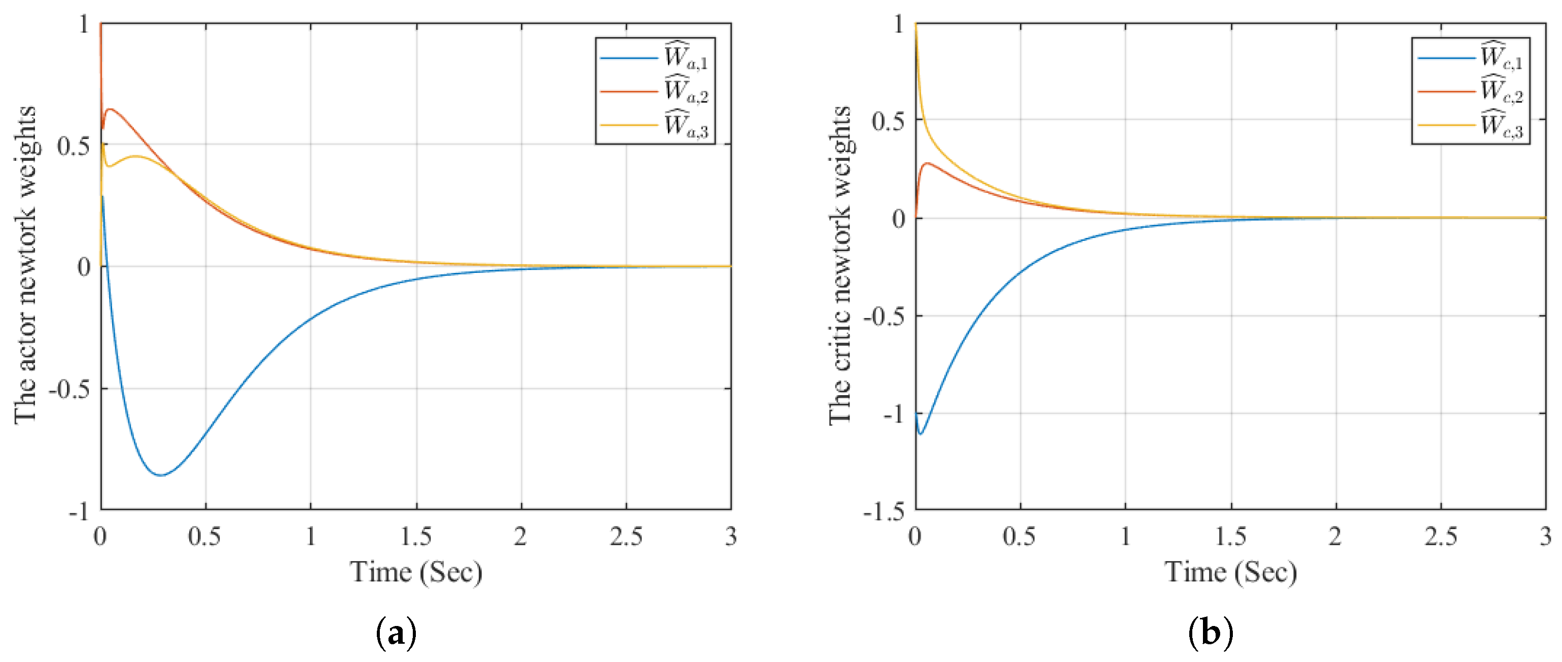
The critic and actor network weight vectors are defined as ${\widehat{W}}_c={\left[{\widehat{W}}_{c,1},{\widehat{W}}_{c,2},{\widehat{W}}_{c,3}\right]}^T$ and ${\widehat{W}}_a={\left[{\widehat{W}}_{a,1},{\widehat{W}}_{a,2},{\widehat{W}}_{a,3}\right]}^T$, respectively. The activation function vector is given by $\Phi \left(\overline{z}\right)={\left[z_1^2,z_1{z}_2,z_2^2\right]}^T$. The learning rates and regularization parameters for the training laws of both the critic and actor (15) and (16) are set to ${\gamma }_c=3$, ${\gamma }_a=5$, and $\sigma =1$. The weight vectors are initialized to ${\widehat{W}}_c\left(0\right)={\left[-1,0,1\right]}^T$ and ${\widehat{W}}_a\left(0\right)={\left[0,1,0\right]}^T$.

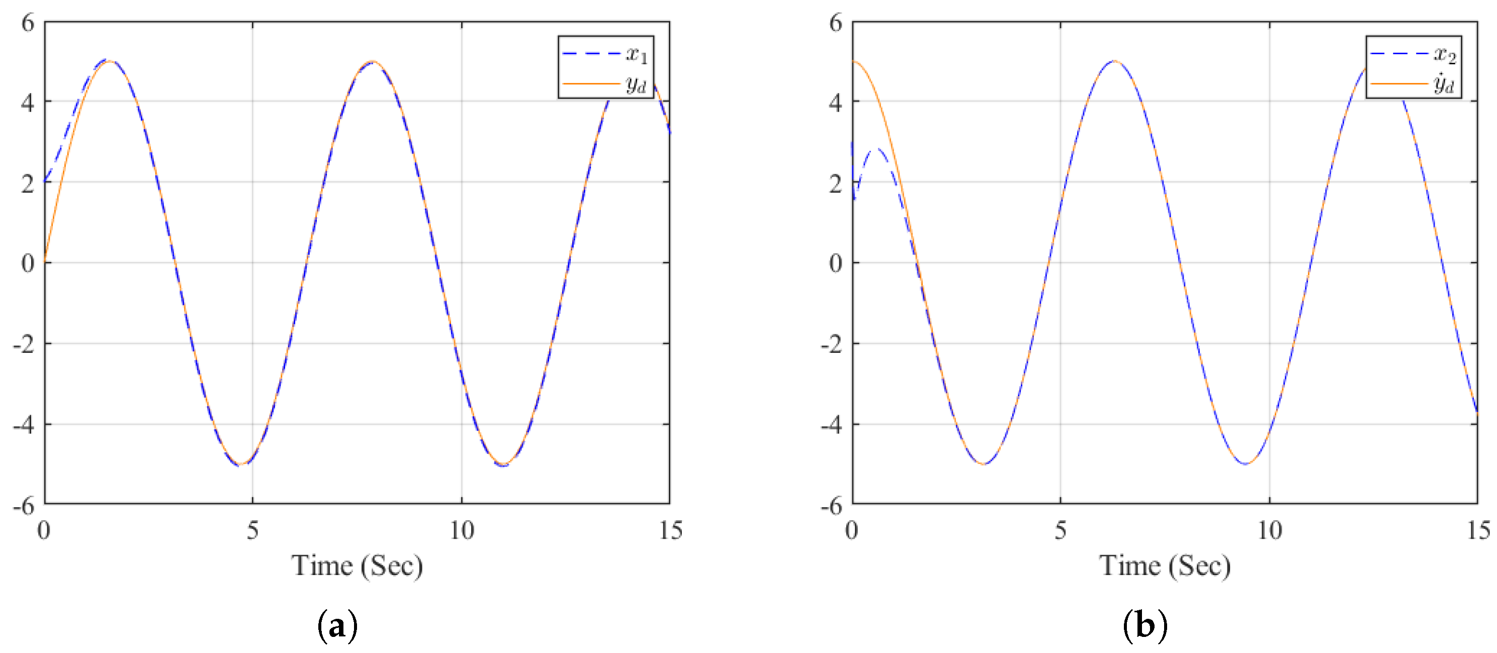
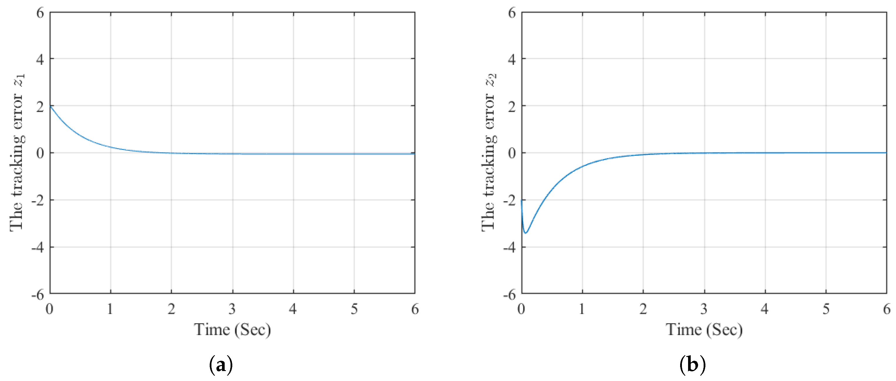
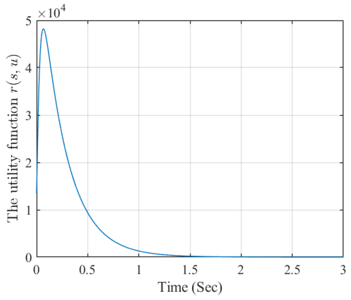
The simulation results are presented in Figure 1, Figure 2, Figure 3 and Figure 4. Specifically, Figure 1 shows that the states $x_1\left(t\right)$ and $x_2\left(t\right)$ closely follow the reference trajectories $y_d$ and its derivative ${\dot{y}}_d$, respectively. The corresponding tracking errors $z_1$ and $z_2$, shown in Figure 2, converge to zero. Furthermore, the neural network weights for the actor and critic remain bounded, as illustrated in Figure 3. Finally, the evolution of the utility function is depicted in Figure 4. Compared with the simulation results in [34], the method proposed in this paper achieves a superior tracking performance.

The performance of our proposed algorithm is first evaluated in Example 1 through a comparative study with the algorithm in [34]. Its adaptability is then examined in Example 2 using a more complex, practical robotic arm system. This system is integrated with commercial servo actuators, which are responsible for converting electrical control signals into joint movements.

Example 2.

This example considers a single-link robotic arm system with flexible joints. In the case of ignoring damping, its nonlinear dynamic equations are given by [37]:

$$\begin{array}{cc}\hfill & I{\ddot{q}}_1+MgLsin\left(q_1\right)+k(q_1+q_2)=0,\hfill \\ & J{\ddot{q}}_2-k(q_1-q_2)=u,\hfill \end{array}$$

(43)

where $q_1$ and $q_2$ represent angular positions ($q_1$ is the system output), I and J are moments of inertia, k is the spring constant, M is the total mass, L is the distance, and u is the torque input.

The above Equation (43) can be transformed to the standard form:

$$\begin{array}{cc}\hfill & {\dot{x}}_1\left(t\right)=x_2\left(t\right),\hfill \\ & {\dot{x}}_2\left(t\right)=x_3\left(t\right),\hfill \\ & {\dot{x}}_3\left(t\right)=x_4\left(t\right),\hfill \\ & {\dot{x}}_4\left(t\right)=-{\displaystyle \frac{MgL}{I}}\left(cos\left(x_1\left(t\right)\right)+{\displaystyle \frac{k}{I}}+{\displaystyle \frac{k}{J}}\right)x_3\left(t\right)+{\displaystyle \frac{MgL}{I}}\left(x_2^2\left(t\right)-{\displaystyle \frac{k}{J}}\right)sin\left(x_1\left(t\right)\right)+{\displaystyle \frac{k}{IJ}}u,\hfill \end{array}$$

(44)

where $x_1=q_1$, $x_2={\dot{q}}_1$, $x_3=-{\displaystyle \frac{MgL}{I}}sin\left(q_1\right)-{\displaystyle \frac{k}{I}}(q_1-q_2)$, and $x_4=-{\displaystyle \frac{MgL}{I}}{\dot{q}}_{1}cos\left(q_1\right)-{\displaystyle \frac{k}{I}}({\dot{q}}_1-{\dot{q}}_2)$

The parameter values of the robotic arm system are set to k = 31 [N m/rad], I = 0.031 [kg m²], J = 0.004 [kg m²], g = 9.81 [m/s²], M = 0.4 [kg], and L = 0.2 [m].

Given the reference trajectory $y_d\left(t\right)=sin\left(2.5t\right)$, the tracking errors can be calculated:

$$\begin{array}{cc}\hfill & z_1\left(t\right)=x_1\left(t\right)-sin\left(2.5t\right),\hfill \\ & z_2\left(t\right)=x_2\left(t\right)-2.5cos\left(2.5t\right),\hfill \\ & z_3\left(t\right)=x_3\left(t\right)+6.25sin\left(2.5t\right),\hfill \\ & z_4\left(t\right)=x_4\left(t\right)+15.625cos\left(2.5t\right).\hfill \end{array}$$

(45)

The error dynamics derived in (44) are

$$\begin{array}{cc}\hfill {\dot{z}}_1\left(t\right)& =z_2\left(t\right),\hfill \\ \hfill {\dot{z}}_2\left(t\right)& =z_3\left(t\right),\hfill \\ \hfill {\dot{z}}_3\left(t\right)& =z_4\left(t\right),\hfill \\ \hfill {\dot{z}}_4\left(t\right)& =-{\displaystyle \frac{MgL}{I}}\left(cos(z_1\left(t\right)+sin\left(2.5t\right))+{\displaystyle \frac{k}{I}}+{\displaystyle \frac{k}{J}}\right)(z_3\left(t\right)-6.25sin\left(2.5t\right))\hfill \\ & +{\displaystyle \frac{MgL}{I}}\left({(z_2\left(t\right)+2.5cos\left(2.5t\right))}^2-{\displaystyle \frac{k}{J}}\right)sin(z_1\left(t\right)+sin\left(2.5t\right))+{\displaystyle \frac{k}{IJ}}u\hfill \\ \hfill & -39.0625sin\left(2.5t\right)\hfill \end{array}$$

(46)

Based on (3), the sliding mode variable is designed as

$$s\left(t\right)=z_1\left(t\right)+z_2\left(t\right)+2z_3\left(t\right)+z_4\left(t\right).$$

(47)

The activation function vector is given by

$$\begin{array}{cc}\hfill \Phi \left(\overline{z}\right)=& [z_1^3,z_1^2{z}_2,z_1^2{z}_3,z_1^2{z}_4,z_1{z}_2^2,z_1{z}_3^2,z_1{z}_4^2,z_1{z}_2{z}_3,z_1{z}_2{z}_4,\hfill \\ & z_1{z}_3{z}_4,z_2^3,z_2^2{z}_3,z_2^2{z}_4,z_2{z}_3^2,z_2{z}_4^2,z_2{z}_3{z}_4,z_3^3,z_3^2{z}_4,z_3{z}_4^2,z_4^3{]}^T.\hfill \end{array}$$

The initial states are $x_1\left(0\right)=5$, $x_2\left(0\right)=1$, $x_3\left(0\right)=2$ and $x_4\left(0\right)=0.3$. The weight vectors are initialized to

$$\begin{array}{c}\hfill {\widehat{W}}_c\left(0\right)={\left[-1,0,1,2,0,1,0,0,1,1,1,1,0,0,1,1,2,0,-1,0\right]}^T\end{array}$$

and

$$\begin{array}{c}\hfill {\widehat{W}}_a\left(0\right)={\left[0,5,0,5,0,2,0,8,0,3,4,0,-2,0,6,2,2,3,0,5\right]}^T.\end{array}$$

The design parameters are set to ${\gamma }_u=30$, ${\gamma }_c=3$, ${\gamma }_a=5$, and $\sigma =1$.

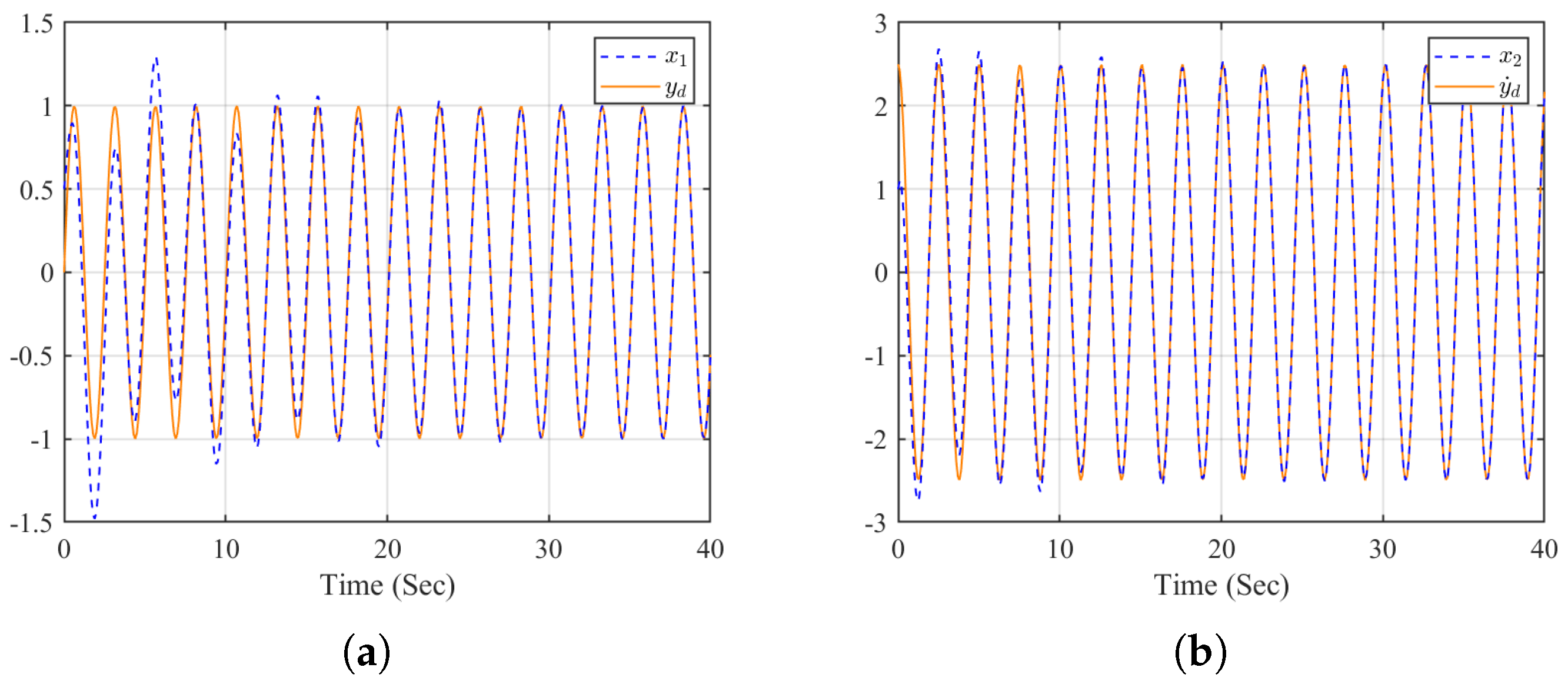
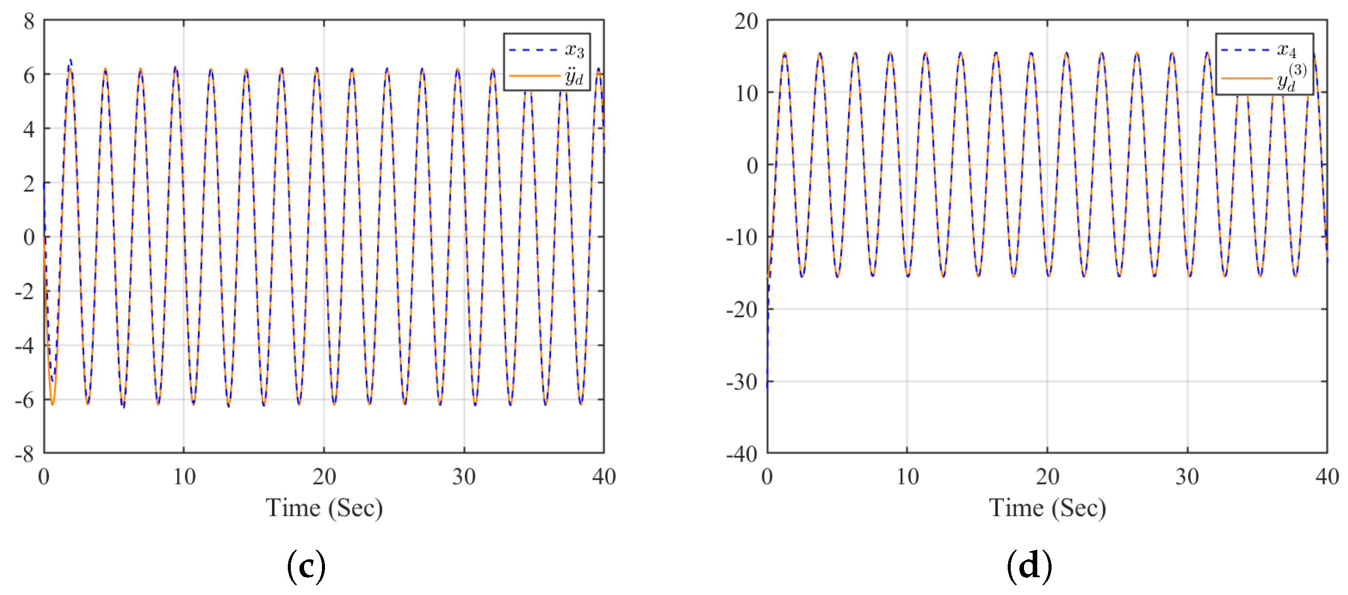
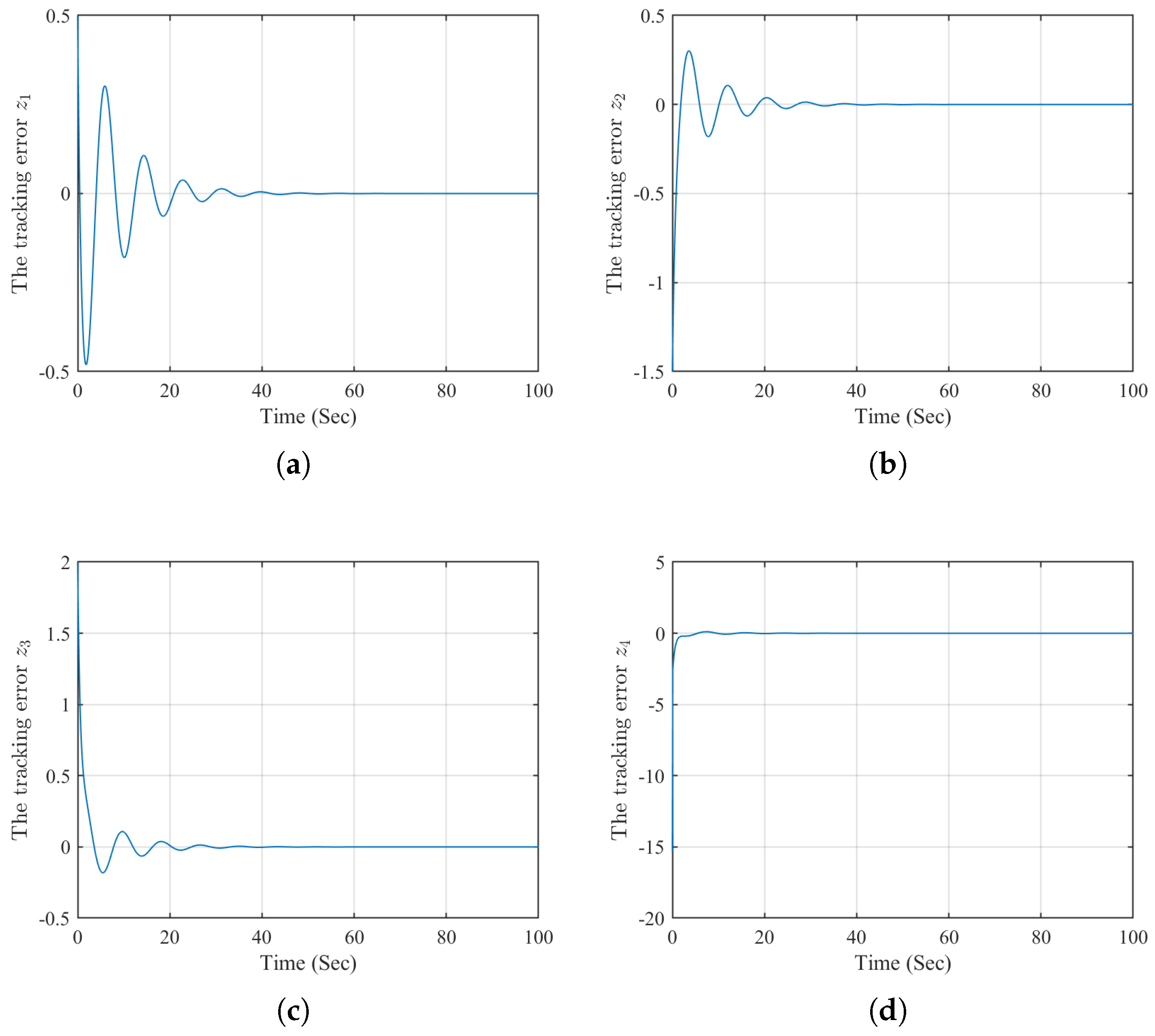
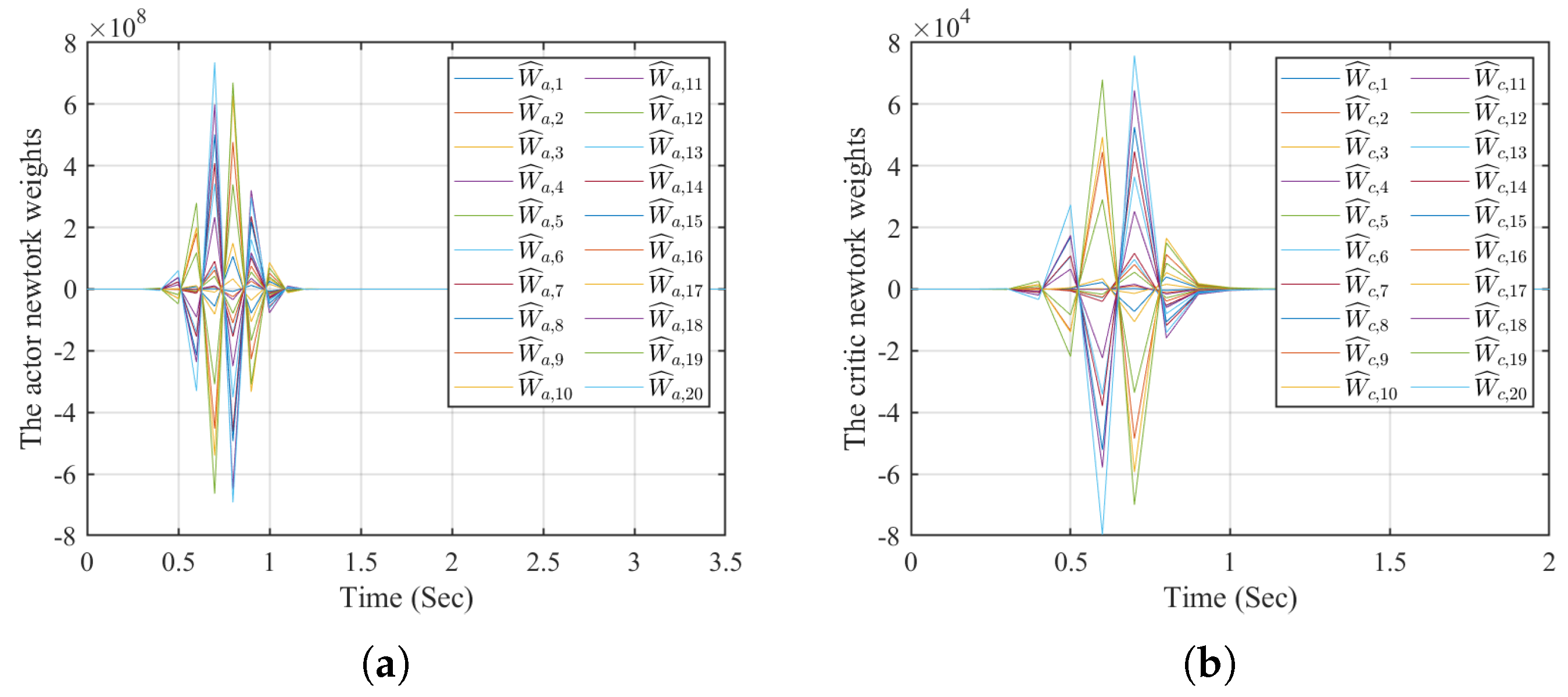
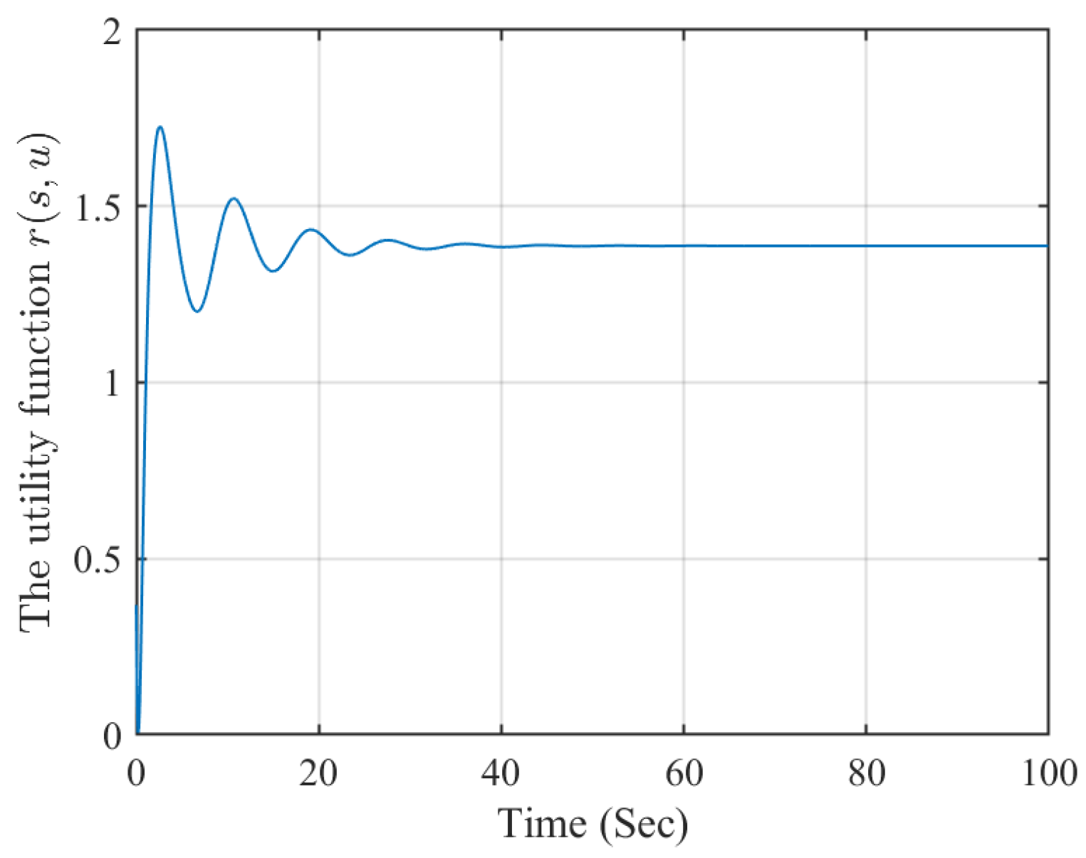
The simulation results of Example 2 are presented in Figure 5, Figure 6, Figure 7 and Figure 8. As shown in Figure 5, the states $x_1\left(t\right)$, $x_2\left(t\right)$, $x_3\left(t\right)$, and $x_4\left(t\right)$ closely follow the reference trajectory $y_d$ and its derivatives of various orders ${\dot{y}}_d$, ${\ddot{y}}_d$, and $y_d^{\left(3\right)}$, respectively. The corresponding tracking errors $z_1$, $z_2$, $z_3$, and $z_4$, depicted in Figure 6, converge to a small neighborhood of zero. Furthermore, Figure 7 demonstrates that the neural network weights for both the actor and critic remain bounded. Finally, the evolution of the utility function is shown in Figure 8. These results demonstrate that the proposed high-order tracking control scheme for canonical nonlinear systems maintains the boundedness of the error signal while ensuring accurate tracking of each system state to its corresponding reference signal.

6. Conclusions

This paper proposes an SMS-based adaptive optimal tracking control scheme, utilizing an NN-based RL approach, for a class of high-order nonlinear systems with partial unknowns. A cost function defined in terms of the SMS is constructed to derive the optimal control law. Accordingly, the HJB equation is addressed within an actor–critic NN framework. Leveraging the inherent relationship between the SMS and the tracking errors significantly simplifies the computational process. Under the premise of ensuring the stability of the closed-loop system, the update law of the actor–critic network is indirectly derived under the condition that a simple function is zero, without the need for the persistence excitation condition. Furthermore, the proposed design requires no prior knowledge of the internal system dynamics. Meanwhile, the proposed method offers a significant advantage over [34] by eliminating the need for a Riccati-like equation. The comparative simulation results demonstrate the superior tracking performance of the proposed scheme over existing methods.

The inadequacy of this method lies in two of its aspects: (1) The control gain of the research system is constant. However, in most practical engineering applications, the control gain often changes with the state, so we will study the case where the control gain changes with the state, even in the case of unknown dynamics. (2) The performance of the closed-loop system and the learning efficiency are hig y dependent on the selection of the SMS parameter $k_j$. Although these parameters satisfy the Hurwitz condition to ensure stability, their specific values need to be empirically balanced among the convergence speed, control energy consumption, and robustness, lacking a systematic tuning method.

References

1. Li, P.; Duan, G.; Zhang, B.; Wang, P.; Wang, Y. High-Order Fully Actuated Approach for Output Tracking Control of Flexible Servo Systems Subject to Uncertainties and Disturbances. IEEE Trans. Ind. Electron. 2025, 72, 9433–9443. [Google Scholar] [CrossRef]
2. Bu, X.; Qi, Q. Fuzzy optimal tracking control of hypersonic flight vehicles via single-network adaptive critic design. IEEE Trans. Fuzzy Syst. 2020, 30, 270–278. [Google Scholar] [CrossRef]
3. Lee, J.; Chang, P.H.; Jin, M. Adaptive integral sliding mode control with time-delay estimation for robot manipulators. IEEE Trans. Ind. Electron. 2017, 64, 6796–6804. [Google Scholar] [CrossRef]
4. Wang, C.; Liu, Z.; Sun, S.; Wang, Z.; Ma, K.; Mao, Q.; Xue, X.; Chen, X.; Zhao, K.; Hu, T. Trajectory tracking of a mobile robot in underground roadways based on hierarchical model predictive control. Actuators 2026, 15, 47. [Google Scholar] [CrossRef]
5. Voos, H. Nonlinear control of a quadrotor micro-UAV using feedback-linearization. In Proceedings of the 2009 IEEE International Conference on Mechatronics, Malaga, Spain, 14–17 April 2009; pp. 1–6. [Google Scholar]
6. Bonna, R.; Camino, J.F. Trajectory tracking control of a quadrotor using feedback linearization. In Proceedings of the International Symposium on Dynamic Problems of Mechanics, Natal, Brazil, 22–27 February 2015; Volume 1. [Google Scholar]
7. Yousefizadeh, S.; Bendtsen, J.D.; Vafam, N.; Khooban, M.H.; Blaabjerg, F.; Dragičević, T. Tracking control for a DC microgrid feeding uncertain loads in more electric aircraft: Adaptive backstepping approach. IEEE Trans. Ind. Electron. 2018, 66, 5644–5652. [Google Scholar] [CrossRef]
8. Zhao, K.; Song, Y. Removing the feasibility conditions imposed on tracking control designs for state-constrained strict-feedback systems. IEEE Trans. Autom. Control 2018, 64, 1265–1272. [Google Scholar] [CrossRef]
9. Yu, J.; Ma, Y.; Yu, H.; Lin, C. Adaptive fuzzy dynamic surface control for induction motors with iron losses in electric vehicle drive systems via backstepping. Inf. Sci. 2017, 376, 172–189. [Google Scholar] [CrossRef]
10. Song, Y.D.; Zhou, S. Tracking control of uncertain nonlinear systems with deferred asymmetric time-varying full state constraints. Automatica 2018, 98, 314–322. [Google Scholar] [CrossRef]
11. Wang, Y.; Gu, L.; Xu, Y.; Cao, X. Practical tracking control of robot manipulators with continuous fractional-order nonsingular terminal sliding mode. IEEE Trans. Ind. Electron. 2016, 63, 6194–6204. [Google Scholar] [CrossRef]
12. Qiao, L.; Zhang, W. Adaptive non-singular integral terminal sliding mode tracking control for autonomous underwater vehicles. IET Control Theory Appl. 2017, 11, 1293–1306. [Google Scholar] [CrossRef]
13. Hwang, C.L.; Chiang, C.C.; Yeh, Y.W. Adaptive fuzzy hierarchical sliding-mode control for the trajectory tracking of uncertain underactuated nonlinear dynamic systems. IEEE Trans. Fuzzy Syst. 2013, 22, 286–299. [Google Scholar] [CrossRef]
14. Zhang, H.; Wang, H.; Niu, B.; Zhang, L.; Ahmad, A.M. Sliding-mode surface-based adaptive actor–critic optimal control for switched nonlinear systems with average dwell time. Inf. Sci. 2021, 580, 756–774. [Google Scholar] [CrossRef]
15. Zhao, H.; Zhao, N.; Zong, G.; Zhao, X.; Xu, N. Sliding-mode surface-based approximate optimal control for nonlinear multiplayer Stackelberg-Nash games via adaptive dynamic programming. Commun. Nonlinear Sci. Numer. Simul. 2024, 132, 107928. [Google Scholar] [CrossRef]
16. Zhang, H.; Zhao, X.; Wang, H.; Zong, G.; Xu, N. Hierarchical sliding-mode surface-based adaptive actor–critic optimal control for switched nonlinear systems with unknown perturbation. Trans. Neural Netw. Learn. Syst. 2022, 35, 1559–1571. [Google Scholar] [CrossRef]
17. Huang, J.; Xu, D.; Li, Y.; Zhang, X.; Zhao, J. Inverse reinforcement learning for discrete-time linear systems based on inverse optimal control. ISA Trans. 2025, 163, 108–119. [Google Scholar] [CrossRef] [PubMed]
18. Modares, H.; Lewis, F.L. Optimal tracking control of nonlinear partially-unknown constrained-input systems using integral reinforcement learning. Automatica 2014, 50, 1780–1792. [Google Scholar] [CrossRef]
19. Xu, D.; Wang, Q.; Li, Y. Optimal guaranteed cost tracking of uncertain nonlinear systems using adaptive dynamic programming with concurrent learning. Int. J. Control Autom. Syst. 2020, 18, 1116–1127. [Google Scholar] [CrossRef]
20. Na, J.; Lv, Y.; Zhang, K.; Zhao, J. Adaptive identifier-critic-based optimal tracking control for nonlinear systems with experimental validation. IEEE Trans. Syst. Man Cybern. Syst. 2020, 52, 459–472. [Google Scholar] [CrossRef]
21. Radac, M.B.; Chirla, D.P. Near real-time online reinforcement learning with synchronous or asynchronous updates. Sci. Rep. 2025, 15, 17158. [Google Scholar] [CrossRef] [PubMed]
22. Jiang, Y.; Liu, L.; Feng, G. Adaptive optimal tracking control of networked linear systems under two-channel stochastic dropouts. Automatica 2024, 165, 111690. [Google Scholar] [CrossRef]
23. Radac, M.B.; Borlea, A.I. Virtual state feedback reference tuning and value iteration reinforcement learning for unknown observable systems control. Energies 2021, 14, 1006. [Google Scholar] [CrossRef]
24. Wen, G.; Chen, C.P.; Ge, S.S.; Yang, H.; Liu, X. Optimized adaptive nonlinear tracking control using actor–critic reinforcement learning strategy. IEEE Trans. Ind. Inform. 2019, 15, 4969–4977. [Google Scholar] [CrossRef]
25. Wang, N.; Gao, Y.; Zhao, H.; Ahn, C.K. Reinforcement learning-based optimal tracking control of an unknown unmanned surface vehicle. IEEE Trans. Neural Netw. Learn. Syst. 2020, 32, 3034–3045. [Google Scholar] [CrossRef]
26. Shi, H.; Yang, C.; Peng, B.; Su, C.; El-Sherbeeny, A.M.; Li, Z. Robust predictive fault-tolerant control based on signal compensation for nonlinear industrial processes with partial actuator failures. Int. J. Control 2026, 314, 131655. [Google Scholar] [CrossRef]
27. Zhang, H.; Zhang, K.; Cai, Y.; Han, J. Adaptive fuzzy fault-tolerant tracking control for partially unknown systems with actuator faults via integral reinforcement learning method. IEEE Trans. Fuzzy Syst. 2019, 27, 1986–1998. [Google Scholar] [CrossRef]
28. Zhuang, H.; Zhou, H.; Shen, Q.; Wu, S.; Razoumny, V.Y.; Razoumny, Y.N. Optimal robust online tracking control for space manipulator in task space using off-policy reinforcement learning. Aerosp. Sci. Technol. 2024, 153, 109446. [Google Scholar] [CrossRef]
29. Wu, T.; Zhang, Y.; Yang, X.; Ye, H.; Xiang, Z. Predefined-time nearly optimal trajectory tracking control for autonomous surface vehicles with unknown dynamics. Ocean. Eng. 2025, 327, 121021. [Google Scholar] [CrossRef]
30. Wen, G.; Ge, S.S.; Tu, F. Optimized backstepping for tracking control of strict-feedback systems. IEEE Trans. Neural Netw. Learn. Syst. 2018, 29, 3850–3862. [Google Scholar] [CrossRef] [PubMed]
31. Liu, Y.; Zhu, Q.; Wen, G. Adaptive tracking control for perturbed strict-feedback nonlinear systems based on optimized backstepping technique. IEEE Trans. Neural Netw. Learn. Syst. 2020, 33, 853–865. [Google Scholar] [CrossRef]
32. Huang, Z.; Bai, W.; Li, T.; Long, Y.; Chen, C.P.; Liang, H.; Yang, H. Adaptive reinforcement learning optimal tracking control for strict-feedback nonlinear systems with prescribed performance. Inf. Sci. 2023, 621, 407–423. [Google Scholar] [CrossRef]
33. Yuan, H.; Cao, L.; Lin, W.; Xiao, W.; Li, X. Learning-observer-based fixed-time optimal tracking control for robotic manipulators with full-state constraints. Neurocomputing 2025, 642, 130186. [Google Scholar] [CrossRef]
34. Wen, G.; Niu, B. Optimized tracking control based on reinforcement learning for a class of high-order unknown nonlinear dynamic systems. Inf. Sci. 2022, 606, 368–379. [Google Scholar] [CrossRef]
35. Song, Y.; Wang, Y.; Holloway, J.; Krstic, M. Time-varying feedback for regulation of normal-form nonlinear systems in prescribed finite time. Automatica 2017, 83, 243–251. [Google Scholar] [CrossRef]
36. Zhu, J.; Wen, G.; Veluvolu, K.C. Optimized backstepping consensus control using adaptive observer-critic–actor reinforcement learning for strict-feedback multi-agent systems. J. Frankl. Inst. 2024, 361, 106693. [Google Scholar] [CrossRef]
37. Hušek, P. Adaptive sliding mode control with moving sliding surface. Appl. Soft Comput. 2016, 42, 178–183. [Google Scholar] [CrossRef]
38. Dao, P.N.; Phung, M.H. Nonlinear robust integral based actor–critic reinforcement learning control for a perturbed three-wheeled mobile robot with mecanum wheels. Comput. Electr. Eng. 2025, 121, 109870. [Google Scholar] [CrossRef]
39. Lin, J.; Wang, M.; Yan, H.; Yang, W. Prescribed-Time Optimal Tracking Control for a Class of Stochastic Systems Using Reinforcement Learning. J. Frankl. Inst. 2025, 362, 107881. [Google Scholar] [CrossRef]
Figure 1. The tracking performances: (a) The state x 1 tracking performance; (b) The state x 2 tracking performance.
Actuators 15 00138 g001
Figure 2. The tracking errors: (a) The tracking error z 1 ; (b) The tracking error z 2 .
Actuators 15 00138 g002
Figure 3. The actor and critic network weights: (a) The actor network weight W ^ a ; (b) The critic network weight W ^ c .
Actuators 15 00138 g003
Figure 4. The utility function r.
Actuators 15 00138 g004
Figure 5. The tracking performances: (a) The state x 1 tracking performance; (b) The state x 2 tracking performance; (c) The state x 3 tracking performance; (d) The state x 4 tracking performance.
Actuators 15 00138 g005aActuators 15 00138 g005b
Figure 6. The tracking errors: (a) The tracking error z 1 ; (b) The tracking error z 2 ; (c) The tracking error z 3 ; (d) The tracking error z 4 .
Actuators 15 00138 g006
Figure 7. The actor and critic network weights: (a) The actor network weight W ^ a ; (b) The critic network weight W ^ c .
Actuators 15 00138 g007
Figure 8. The utility function r.
Actuators 15 00138 g008
Disclaimer/Publisher’s Note: The statements, opinions and data contained in all publications are solely those of the individual author(s) and contributor(s) and not of MDPI and/or the editor(s). MDPI and/or the editor(s) disclaim responsibility for any injury to people or property resulting from any ideas, methods, instructions or products referred to in the content.