Abstract
The huge growth in the utilisation of six-axis robots in various technological applications in production calls for a detailed focus on the process of preparing Numerical Control (NC) programmes for effective robot control. Considerable attention is currently being paid to optimisation by increasing stiffness, but there is also a need to focus on reducing energy consumption in robot control. Focusing on reducing energy consumption is highly justified given the widespread adoption of robotic systems across diverse manufacturing technologies and the significant potential for application. This is particularly relevant today, when minimising production costs is a critical industrial objective. A redundant degree of freedom—which is the possibility to rotate around the end-effector axis and thus influence the adjustment of the rotation of the individual robot joints—can be used for this purpose. Therefore, this paper exploits this redundant degree of freedom to set up a proper robot configuration that reduces energy consumption. The user-friendly solution, including the algorithm design and processing through a function, could be effectively implemented within an industry-standard post-processor solution for generating NC programmes for robots. This solution is unique as it is used for the optimisation of the working section of the toolpaths, where continuous control of the end-effector movement during manufacturing operations occurs. The solution was verified on a KUKA KR60 HA robot; however, it is applicable to any industrial six-axis robot. Substantial energy savings were obtained in multi-axis toolpath operations, with a 7.5% reduction in total energy consumption when using the optimised NC programme.
1. Introduction
As the level of robotisation continues to rise, so does the range of technological applications for robotic systems. One notable area of application is conventional subtractive manufacturing, where industrial robots have proven particularly useful in the manufacturing of large and bulky components. Robotic machining offers an efficient solution for the production of complex parts from materials such as polymers, composites and aluminium alloys. Robots carrying processing heads (end-effectors) can perform a variety of operations, including milling, grinding, deburring and other multi-axis processes, with high repeatability and flexibility.
The primary advantages of using robots in machining are their extensive working range and lower acquisition cost compared to conventional CNC machines. However, due to their relatively low static stiffness and high dynamic compliance, industrial robots are generally not employed in high-power machining applications, where it is difficult to consistently achieve the required precision [1]. To address these limitations, optimisation methods are being developed to enhance the functional characteristics of robotic control. In particular, advanced optimisation algorithms are being integrated into the pre-processing phase of robot programming to improve machining accuracy.
Brunete et al. [2] proposed an advanced model for robotic stiffness that accounts for the torsional stiffness of individual robot sub-joints, with sub-stiffness values derived from static stiffness measurements. They also introduced a cutting process model that includes the calculation of cutting forces and machining stability. Using these two models in offline toolpath optimisation enables the adjustment of the target end-effector coordinates to achieve a compensated machining position, thereby enhancing accuracy. In addition, advanced calibration techniques—such as those employing machine learning and neural networks for geometric error correction—have been shown to further improve robotic control system accuracy, as demonstrated by Wang et al. [3]. A notable trend in robotic machining involves the processing of thin-walled components, where the robot functions as a support device to increase overall system stability and accuracy. This concept has been validated in both machine tool applications, as described by Ozturk et al. [4], and dual-robot cooperative systems, where one robot is equipped with a milling spindle and the other with a support mechanism, as detailed by Zhang et al. [5]. An unconventional but innovative approach involves the use of two robots machining opposite to each other, as presented by Wang et al. [6]. This setup incorporates vibration analysis and dynamic modelling to enhance machining stability.
Robotic operation optimisation must also address vibration suppression, which is essential for achieving high-quality surface finishes. Vibrations can be mitigated through the selection of appropriate cutting parameters, improved tool clamping and the use of passive or active damping systems on the robot end-effector, as explored by Yuan et al. [7] and Sun et al. [8]. Strategies for optimising spindle speed to eliminate chatter and enhance process stability—which is particularly important given the high dynamic compliance of robots—are discussed by Cordes et al. [9] and Xin et al. [10]. Low-frequency oscillations, typically in the range of 10–20 Hz, have been analysed using various approaches, as presented by Wu et al. [11] and Busch et al. [12]. Liu et al. [13] proposed a process model for chatter detection in robotic machining, along with an optimisation algorithm that adjusts the robot’s joint configuration to improve the surface roughness of the machined part. Liu et al. [14] further developed an extended method for identifying self-excited chatter in robotic machining. In this approach, the tool–workpiece system is modelled as a mass–spring system, where the maximum allowable depth of cut is dependent on the robot’s kinematic configuration. More compliant configurations result in reduced stability and a lower allowable depth of cut.
Six-axis industrial robots possess one additional degree of freedom—often referred to as a redundant degree of freedom—beyond what is required for five-axis machining. This redundancy allows for multiple kinematically valid joint configurations during motion, enabling the selection of specific joint rotations based on the machining context, as discussed by Zhu et al. [15]. While the primary use of this redundancy in robotic control is typically to avoid collisions, optimisation algorithms have been developed to exploit specific joint configurations to increase static stiffness. This, in turn, reduces the deviation between the actual and desired end-effector positions during machining operations, as shown by Chen et al. [16]. A key approach involves utilising the redundant rotational degree of freedom of the end-effector about its own axis to identify configurations that maximise overall system stiffness while maintaining the relative position between the tool and the workpiece. This concept is demonstrated in studies by Xiong et al. [17] and Schneider et al. [18]. A similar method was proposed by Guo et al. [19], who focused on increasing stiffness in the direction of the primary cutting force during the drilling of large aerospace components. Kratena et al. [20] implemented a genetic algorithm to find the best settings of the redundant degree of freedom so that the workpiece’s optimal position relative to the robot has the highest stiffness. Comparative studies of static stiffness and dynamic compliance models, such as the study by Cvitanic et al. [21], suggest that when machining parameters are appropriately set, the performance differences between these models are minimal, provided that the robot’s natural frequency remains sufficiently distant from the excitation frequency acting on the end-effector. Ratiu et al. [22] presented additional applications of optimisation strategies leveraging the robot’s redundant degree of freedom, including techniques aimed at maximising productivity or minimising unnecessary reversal movements. Erdős et al. [23] highlighted the use of the redundant degree of freedom in robotic systems for optimising control strategies aimed at reducing production cycle time in laser welding applications. Their proposed optimisation algorithm identifies joint rotation configurations that minimise overall production time. Similarly, Flacco et al. [24] demonstrated how actuator accelerations and torques can be effectively managed by optimising the velocity profiles of individual robot axes. This approach may also be applied to energy optimisation by minimising abrupt changes in acceleration and torque.
A study by Garcia et al. [25] investigates key contributors to energy consumption in robotic operations, reporting, for example, that up to 28% of a robot’s total energy use can occur during idle states. Certain robot postures are associated with higher energy demands due to inertia and gravitational effects; hence, it is advisable to minimise servo motor activation time when a robot is stationary. Khalaf et al. [26] proposed a novel approach to robotic structure design based on regenerative drive mechanisms, which utilise ultracapacitors to store and recover energy. Their work introduces new control and modelling techniques that enhance energy regeneration efficiency and facilitate direct energy transfer between robot joints. Finally, Soori et al. [27] provided a comprehensive overview of the key factors involved in developing energy-efficient robotic systems. Within the context of NC programme design, they emphasised the importance of minimising unnecessary motions, optimising toolpaths and controlling movement speeds. The use of simulation tools and machine learning algorithms was highlighted as an effective means of identifying energy-efficient toolpaths for end-effector motion relative to the workpiece. Feng et al. [28] presented an approach that leverages the multiple possible joint rotation configurations available to industrial robots during point-to-point motion in manipulation tasks. By optimising joint rotations and applying global task scheduling, the method enables more efficient energy utilisation in cyclic industrial operations. The proposed strategy is adaptable to real-world production environments and holds potential for integration into production planning software. In a related study, Zhou et al. [29] developed a comprehensive model of energy consumption for robotic laser operations, incorporating both robotic motion and process-specific energy requirements. The model was subsequently simplified to operate within a defined range of robot feed rate, enabling accurate energy consumption predictions while reducing computational complexity. Despite this simplification, the model remains detailed and includes parameters such as joint friction coefficients. An alternative to physics-based modelling is the use of data-driven approaches, which apply machine learning techniques to estimate energy consumption. The key advantage of these models is that they do not require detailed knowledge of the physical parameters of each robotic component. However, these methods depend on the availability of sufficient training data. An example of this approach was provided by Zhang et al. [30], who proposed a machine learning model aimed at identifying optimal robot axis operating parameters such as velocities and accelerations to minimise energy consumption without the need for complex mathematical modelling of robot kinematics and dynamics.
As demonstrated by the reviewed literature, there are several principal approaches for optimising robot control. Most of the work is focused on increasing stiffness during machining. Some papers also deal with optimising control to reduce energy consumption by utilising the robot’s sixth (redundant) degree of freedom to identify optimal joint configurations or minimise energy consumption during point-to-point movements. However, when a robot is required to follow a predefined toolpath continuously—such as during manufacturing operations where the end-effector has to maintain precise motion relative to the workpiece—existing optimisation strategies that exploit redundancy for energy reduction are generally not applicable as they often assume flexibility in the toolpath itself.
To address this gap, this paper proposes a discretisation-based algorithm that utilises the robot’s redundant degree of freedom to identify a joint rotation configuration that minimises energy consumption during continuous toolpath processing operations. The aim is to develop the algorithm to be applicable to any industrial six-axis robot, regardless of the processing technology used (or the specific end-effector used). The prerequisite is that the robotic operation with the specific end-effector allows one to change its orientation around its axis.
2. Discretisation Algorithm Proposal and Implementation
To make the approach effective in practice, the proposed algorithm, along with the function as a complete module, must be easy to implement. Therefore, the design is based on the simplest computational mechanism possible so that it can be as user-friendly as possible when generating NC programmes for the robot.
2.1. Discretisation Function Parameters
The discretisation function is based on using the redundant degree of freedom, which is the angle of rotation about the end effector axis (angle C (Figure 1)).
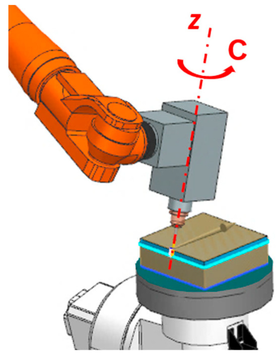
Figure 1.
Redundant degree of freedom.
This variable can generally be a value within the range of 0° to 360° and can be incremented by, for instance, whole degrees or tenths of a degree. Any finer increment will unnecessarily increase the computation time without producing noticeably better results. Therefore, a discretisation approach was adopted in this work. An example of two angular setups of joints based on two values of angle C can be seen in Figure 2. It should be noted that the minimum and maximum values of angle C differ for each specific application due to the specific robot’s working space as well as the specific limits of the given end-effector. Thus, for a given operation, the algorithm loop would only work with a few tens of possible values of the discretised variable. Therefore, the proposed function works with: (a) the C angle range and increment, (b) the range of the limit angles of individual robot joints, and (c) their limit angular velocities and accelerations.
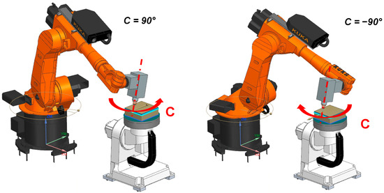
Figure 2.
Example of two angular setups of joints based on two angles of redundant DOF.
The appropriate setting of parameters for robot motion control assumes knowledge of a particular indicator expressing energy consumption. Obviously, it is necessary to calculate the inverse dynamics of the robot, including friction in the joints and other parameters to precisely calculate the electric energy consumption. This is, however, a computationally demanding and complicated solution. A different approach, used in this work, is to use an indicator that only differentiates between studied configurations and does not have to provide precise values of the consumed electrical energy. This direct indicator is the kinetic energy that is required to realise the robot motion or the individual robot arms involved in the overall motion. It is thus the energy of the rotating element. However, it is not necessary to calculate the kinetic energy directly; it is sufficient to make an assessment based on knowledge of the main variable parameters that affect the kinetic energy calculation in order to evaluate the most suitable robot setup. These parameters are the angular velocities of the individual robot joints and the mass parameters of the individual robot links involved in the motion.
2.2. Kinematic Transformation Matrix
To be able to calculate the angular velocities in each robot axis (joints), it is necessary to first derive the specific kinematic transformation matrix. The matrix is related to the specific robot configuration, i.e., the specific degree of freedom. A schematic representation of a six-axis robot kinematic structure can be seen in Figure 3. This kinematic structure also contains the main parameters that are used for the Khalil–Kleinfinger (K-K) notation to derive the transformation matrix. These parameters are as folows:
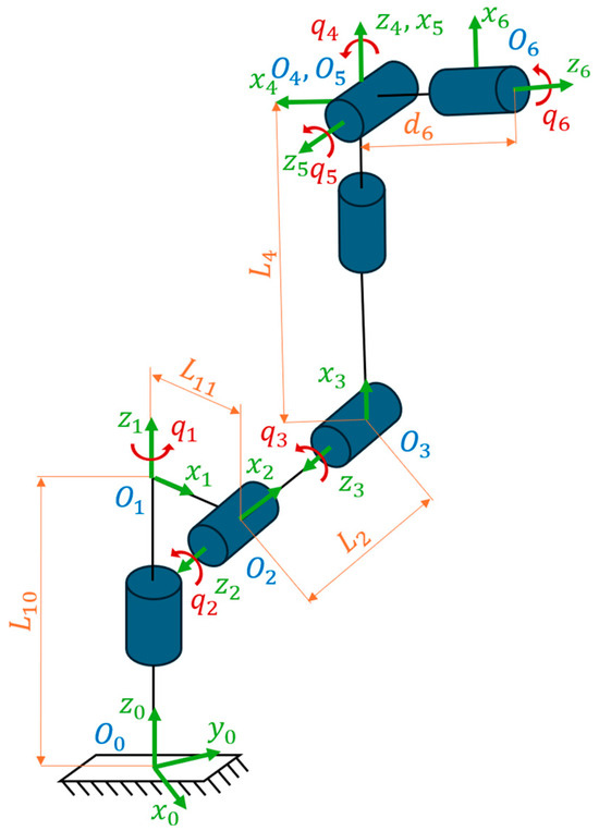
Figure 3.
Kinematic structure and parameters for the K-K notation of a six-axis robot (the following color scheme is used: blue—joint coordinate systems, green—x, y and z axes of joint coordinate systems, red—angles of joints, orange—dimensions of robot parts).
- —angle between the zi−1 and zi axes around the xi−1 axis
- —angle of a specific robot axis (joint)
- —perpendicular distance of the origin Oi−1 from the zi axis
- —distance between origins Oi−1 and Oi
The adopted parameters for the six-axis robot according to the K-K convention can be seen in Table 1, where each robot joint is designated as a value of .

Table 1.
Table of K-K parameters for six-axis robot according to Figure 3.
For the K-K notation, the kinematic transformation matrix has a dimension of 4 × 4 and is a function of the parameters from the K-K table. Its symbolic notation can be seen in (1).
The total kinematic transformation matrix is then determined according to (2).
2.3. Composition of the Jacobian and Calculation of Angular Velocities of the Robot Axes
The Jacobian is a mathematical tool used in robotics to convert velocities in a Cartesian space to velocities in a joint space, i.e., angular velocities of rotational axes. It can also be used to detect singular robot positions, i.e., configurations where the Jacobian matrix is singular (in these cases, the inverse matrix of the Jacobian does not exist). It is important to avoid these positions when planning robot trajectories as they cause large increases in joint velocities and reduce overall positioning accuracy.
In this study, the Jacobian matrix was used only to convert the velocities of the robot flange in Cartesian space to the angular velocities of the robot joints. The Jacobian matrix generally has a dimension of 6 × n, where n corresponds to the number of robot joints. For a six-axis robot, the matrix will have a dimension of 6 × 6. The Jacobian matrix itself is made up of submatrices that can be composed from the data contained in the K-K convention. The conversion of velocity coordinates using the Jacobian is expressed by Equation (3). Vector represents the angular velocities of the robot axes (joints) and vector represents the velocity of the robot flange in Cartesian space. The Jacobian matrix is different for each robot configuration and is a function of the joint rotations.
As already mentioned, the Jacobian is made up of submatrices. These individual submatrices can be seen in (4).
Subsequently, it is necessary to calculate the matrix inverse to it and rewrite Equation (3) in the following form (5):
This calculates all of the robot’s joint angular velocities. This algorithm is implemented using a recursive calculation and can be used to determine the overall robot velocity along working toolpaths programmed in CAM software (Siemens NX CAM system is used in this paper, however it doesn’t matter which CAM system is used).
2.4. Design of the Discretisation Function
Analytical models for predicting the power consumption of robot motion are usually based on Equation (6), which describes the robot’s inverse dynamics. Given a known robot’s articulated axes positions (), velocities () and accelerations (), it is possible to determine the required torques in each of the robot’s articulated axes () to achieve the desired end-effector motion.
is the robot’s inertia matrix, is the matrix of centrifugal and Coriolis terms, is the vector of gravitational forces and represents the torques at the articulated joints. The electric energy consumption (8) can then be calculated from the immediate power value (7) determined by the calculation of the inverse dynamics (required joint torques , motor torques ) and by the motor characteristics (electrical resistance of the motor ; torque constant of the motor ) [31,32]. In case of a trajectory containing a large number of points, where this calculation needs to be performed at each point, the computational power requirements and complexity increase significantly.
In addition, there are other factors that influence energy consumption, like, for example, joint friction. However, this work was motivated by the fact that actual power consumption is strongly related to the actual kinetic energy needed to realise the movement of a specific element. Therefore, the aim was to develop a function that would use energy index as an indicator of actual power consumption, but the calculation was greatly simplified in comparison with the inverse dynamics solution. The formula for calculating the index was derived from the obvious kinetic energy formula for a rotating element (9). The energy index Ek was based on calculating the sum of the particular energy indexes of each robot axis, which are expressed as the product of the angular velocity of the specific robot joint and the constant (10). The constant considers the ratio of the mass of the robot part being moved by a certain joint and the mass of the whole robotic body.
From the perspective of computational complexity, the most suitable way to evaluate the data was to iteratively increase angle C and then evaluate the power consumption index for each toolpath section (specific tool pass). The proposed algorithm can be seen in Figure 4. This procedure is also suitable due to the narrow range of values that angle C can take. Therefore, a simple discretisation approach was chosen, as more complex discretisation methods such as genetic algorithms were not necessary. Furthermore, the data processing method according to the type of movement (working or non-working) within the technological operation needed to be determined. The algorithm loop works with Cutter Location (CL) data generated by the CAM software. This data contains information about the desired position and orientation of the tool (e.g., the end-effector axis) in space. It also contains information about the type of movement, e.g., cutting, arrival, traversal, departure. During working movement, the tool is in contact with the workpiece, while non-working movement only serves for the repositioning of the tool (end-effector) between working sections or the arrival and departure from the material. Therefore, the constant C angle value is used for one whole tool pass (depicted by the purple rectangle in Figure 4), and the C angle value is changed on the transition sections (non-working movements) of the toolpath.
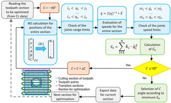
Figure 4.
Discretisation algorithm flowchart.
2.5. Design of the Computational Loop
At the beginning of the calculation, angle C is set to an initial value, e.g., −90 degrees. The IK (inverse kinematic) is then calculated for all points belonging to the working section and the angular constraints are checked. Next, the velocity calculations in each toolpath point are performed and the results are checked to ensure that they are within the boundary conditions. If the kinematic parameters of the joint’s drives are exceeded for any of the points in the section, the corresponding angle C is discarded. Finally, the energy consumption index for the whole section is evaluated depending on one setting of angle C. Angle C is then listed in the matrix along with the corresponding index value. Angle C is then increased by the given step and the calculation is performed again until angle C reaches the limit value, e.g., 90 degrees. A simplified diagram of the discretisation loop can be seen in Figure 5. After all movements of the technological operation have been discretised, the NC programme containing the specific C angle values for each of the tool passes is generated.
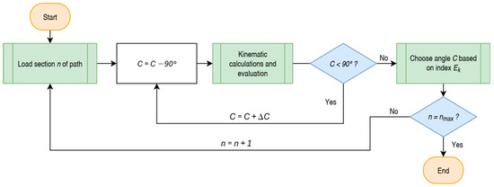
Figure 5.
Discretisation loop diagram.
2.6. Implementation of Velocity Calculation Function in the Discretisation Algorithm
To develop the discretisation algorithm, it was necessary to create a parametric function with input variables that could be called from the parent computational loop (Figure 6). These variables are the complete CL data, which contain the set of the tool tip position (Tool Centre Point—TCP) and orientations in space along with the rotation angle about axis C. These input variables are used to define the tool positions P1 (previous position) and P2 (actual position). Next, the FOR cycle is responsible for the recursive calculation of the joint velocities. In the loop, the translational velocity of the TCP point is first calculated, followed by the angular velocity of the tool frame at the TCP. Afterwards, the conversion to robot flange velocities is performed as described in the previous sections. This is followed by the calculation of the Jacobian matrix. Then, the robot’s actual joint velocities are calculated. After the calculation of the joint velocities for the entire toolpath, the limit velocity and acceleration values are checked. If the limits are exceeded, parameter E2 is output with a value of 1 (or a value of 0, if the limits are not exceeded). This parameter is then exported to the file E2.txt, which is used to evaluate the optimal setting of angle C in the parent loop. At the end of the function, the power consumption index is calculated.
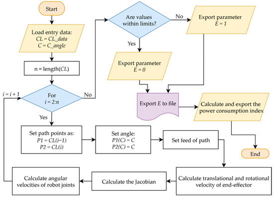
Figure 6.
Flowchart of the velocity calculation function.
2.7. Implementation of the Discretisation Function
An example of the implementation of this function was performed using the Siemens NX CAM system. It is possible to call DLLs (Dynamic Link Libraries) containing external functions when postprocessing CL data to an NC programme directly by the postprocessor. In the case of the proposed algorithm, the DLL contains a programme with a discretisation function. After initialisation, the function contained in the library can be called during postprocessing. A simplified diagram of postprocessor communication with a DLL library can be seen in Figure 7.
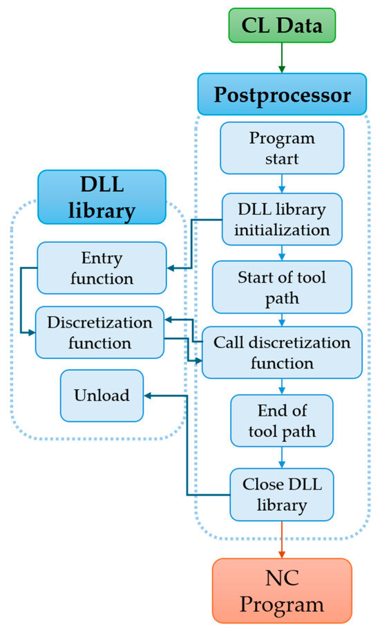
Figure 7.
Simplified implementation of DLL library into the postprocessor.
3. Experimental Verification of the Discretisation Algorithm and Discussion of the Results
The proposed discretisation algorithm was verified in a real application by evaluating its effectiveness in controlling a specific robot through measurements of power consumption during the robot’s operation.
3.1. Description of the Workcell
A six-axis KUKA KR60 HA robot (Germany) with a serial kinematic structure and a spherical wrist was employed for experimental verification. This robot was developed for high-precision applications such as MIG/MAG welding, metal powder welding and machining. According to KUKA specifications, it has a working range of 2033 mm, positioning repeatability of ±0.05 mm, path accuracy of ±0.016 mm and payload capacity of 60 kg.
The robot used for experimental verification is equipped with a CEAD E25 print head, designed for large-format 3D printing, which was also utilised as the end-effector during testing of the discretisation function. A workcell showing the robot and the end-effector is presented in Figure 8 (real robot—left). A simulation model of the robot with a control system emulator was also developed for the purposes of setting up technological operations employing discretisation and subsequent verification of the production process (see Figure 8—right).
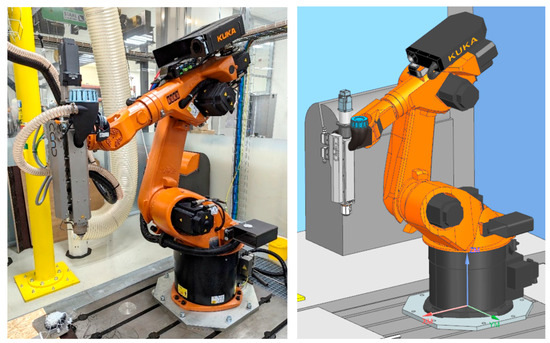
Figure 8.
Robotic cell (left) and corresponding simulation model (right).
The proposed discretisation algorithm was adapted to the specific robot by setting the rotational limits and angular velocity limits of each axis in accordance with the parameters listed in Table 2.
Table 2.
Limits of kinematic parameters of robotic axes.
In this case, the robot was controlled using a Siemens Sinumerik 840D control system, which incorporates a Sinumerik Run MyRobot/Machining extension.
3.2. Verification of the Calculation of Robot Axis Velocities
First, it was necessary to verify the calculation of the velocities of each robot axis. This phase—calculating the velocities of each of the robot’s axes—was crucial for the functionality of the discretisation algorithm.
Although the focus of this paper is primarily on machining applications, the developed algorithm is applicable to any operation involving up to five axes, such as grinding, polishing or bending, as well as 3D printing, laser cutting, welding or waterjet cutting. Therefore, to test the velocity profiles of the machine axes, a simple part involving a five-axis manufacturing operation was designed in Siemens NX CAM software (see Figure 9).
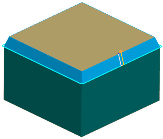
Figure 9.
Test toolpath for verification of the calculation of the velocities.
The predicted velocity characteristics of each axis are shown in Figure 10A. Simultaneously, the NC programme for this toolpath was used for measurement on the actual robot during interpolation using the Trace function available directly within the control system, which can be seen in Figure 10B. The measured data (Figure 10B) and calculated data (Figure 10A) corresponded well. Minor deviations, particularly at points where the robot needed to move the end-effector around sharp corners of the part, were attributed to three main factors. One factor was the difference in the number of data points between the two graphs. The velocity characteristics calculated by the algorithm were based on CL data, which contained significantly fewer points than the machine-measured characteristics, derived from data already interpolated by the control system. A second important factor was the use of the lookahead function in combination with the toolpath interpolation algorithm. The controller used this function to schedule the interpolated toolpath points within a tolerance several NC blocks in advance to maintain the feed rate at a constant value as much as possible along the entire toolpath. A third factor was the specific version of the controller itself, which used a proprietary interpolation algorithm. This included the frequency of interpolation and the algorithm’s characteristics, such as whether it performed additional smoothing (e.g., based on using spline curves). The functionality of a critical component of the discretisation algorithm was validated, allowing verification of the main section of the algorithm.
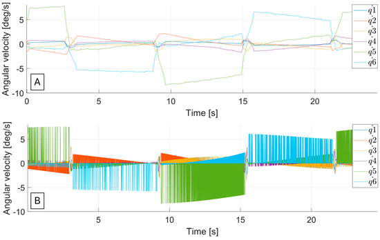
Figure 10.
Velocities of robotic axis (joints) ((A)—prediction, (B)—measurement).
3.3. Verification of Electric Energy Consumption
To verify the functionality of the complete discretisation algorithm, it was necessary to confirm that the specific value of the redundant degree of freedom angle that had been identified actually leads to power savings. This testing also validated that the algorithm correctly distinguishes between working and non-working motions and generates a unique angle C (the redundant degree of freedom) for each pass along the complete toolpath. Power consumption measurements were carried out for two types of toolpaths: three-axis and five-axis. A three-phase power network analyser from Chauvin Arnoux, model Qualistar C.A. 8335, was used to measure power consumption. The analyser was connected directly to the switchboard supplying electricity to the drive inverters of the KUKA KR60 HA robot (see Figure 11).
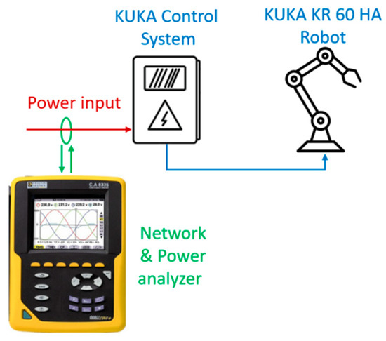
Figure 11.
Analyser connection when measuring power consumption (The figure contains only an example of the device).
3.3.1. Power Consumption Measurement for Three-Axis Operations
The first step involved measuring power consumption during a three-axis operation. For this purpose, a part with a complex surface shape leading to setting up the testing toolpaths was designed (see Figure 12), consisting of cutting sections (light blue) and traverse sections (light green).
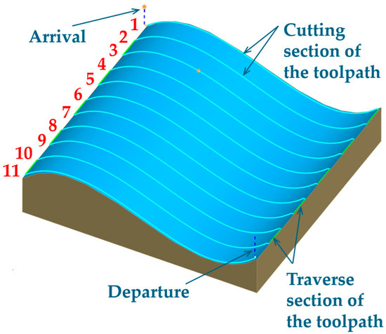
Figure 12.
Test toolpath for measuring power consumption in three-axis machining (Numbers 1–11 in red indicate individual tool passes).
For these toolpaths, CL data were generated using the Siemens NX CAM system and subsequently processed by the discretisation algorithm, which produced an NC programme executable on the robot. The algorithm identified a redundant degree of freedom (DOF) angle of 45° as the option that achieved the lowest energy index Ek (see Table 3). A feed rate of 3000 mm/min was used during the measurements.
Table 3.
Angle C value for 3-axis NC code.
The experiment involved measuring the total input power at the terminals of the junction box housing the inverters for the machine axes, using the aforementioned three-phase electrical analyser. Two NC programmes were run four times each, consecutively in an automatic loop on the robot, and the data were averaged. First, the standard NC programme generated directly by the Siemens NX postprocessor was tested. The averaged data from the four runs were plotted in MATLAB R2025a, where the total electrical energy consumed during the motions was determined by integrating the area under the curve.
Then, the NC programme with angle C calculated according to the discretisation algorithm was executed. The NC programme was again run in a loop, where it was repeated four times. Data processing from the measurement software was carried out in the same way as for the previous code. The characteristics of the measured data can be seen in Figure 13, where the individual tool passes (1–11) corresponding to the partial passes of the toolpath shown in Figure 12 are also visible. When plotting data for both NC programmes, it was necessary to correctly select the sections during which the robot was processing the NC programme and remove the sections where the robot was moving between the four repetitions. This was essential for the evaluation of the total electrical energy consumption by the integration method. With different time window sizes, the x-axis of one of the curves would have been extended and the areas under the graph curves would not have been comparable.
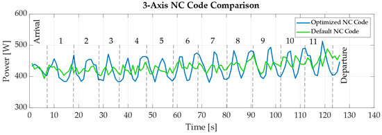
Figure 13.
Power input to the robot inverters when clearing standard and optimised NC programmes (Numbers 1–11 indicate individual tool passes).
From the characteristics of both measurements, it was evident that there was no significant reduction in total electrical energy consumption. The difference in electrical energy consumption between the measurements was approximately 0.65% in favour of the NC programme, with angle C calculated according to the discretisation algorithm. However, this may only have been a measurement error introduced by, for example, the low sampling frequency, which was 1 Hz. During the laboratory measurement itself, the robot in idle mode was found to have an instantaneous power consumption for the inverters of approximately 380 W. During the execution of the proposed operation, the instantaneous power consumption was at most around 500 W. Therefore, the robot did not perform any demanding movements and, thus, almost no change in total electrical energy consumption was measured (see Table 4).
Table 4.
Comparison of measured data for the three-axis operation.
The measured data indicate that for three-axis operations, in which the individual robot axes perform relatively undemanding motions (characterised by large angular changes and velocities), the algorithm does not achieve significant success.
3.3.2. Power Consumption Measurement for Five-Axis Operations
The second measurement involved a manufacturing operation with five-axis toolpaths. For this test, toolpaths with multiple working sections were generated (see Figure 14). CL data were again generated for processing by the discretisation algorithm, alongside a standard NC programme created in Siemens NX.
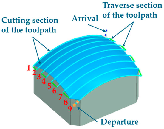
Figure 14.
Test toolpath for measuring power consumption in five-axis manufacturing (Numbers 1–9 in red indicate individual tool passes).
The discretisation algorithm identified a value of −30° for angle C as the option that minimised power consumption (Table 5). A feed rate of 3000 mm/min was used for testing.
Table 5.
Angle C values for 5-axis NC code.
Figure 15A illustrates that in the default state (with the NC programme obtained from the CAM system), there were large rotational changes in the robot’s individual axes (joints). After applying the discretisation algorithm, these angular changes in the robot’s individual axes were significantly reduced, as shown in Figure 15B. The toolpath sections are indicated by red numbers, which correspond to the sections depicted in Figure 14.
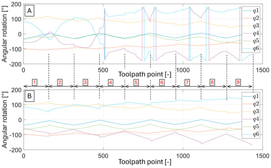
Figure 15.
Movements of robotic axes (joints) along the toolpath ((A)—default, (B)—optimised, Numbers 1–9 in red indicate individual tool passes).
The effect of the discretisation algorithm was also clearly demonstrated in the angular velocity characteristics of the robot’s individual axes (Figure 16). Figure 16A shows the angular velocity characteristics of the robot’s individual axes obtained from the default NC programme as received from the CAM system. The corresponding angular velocity characteristics for the NC programme optimised by the discretisation algorithm, i.e., using the calculated angle C, are presented in Figure 16B. It is evident that the peak velocities were reduced to approximately one-third of those in the default NC programme. These characteristics are further detailed in Figure 16C, which displays the same data as in Figure 16B but with an increased scale on the y-axis. In these detailed characteristics, it is apparent that the velocities of the robot’s individual axes were more uniform compared to the original characteristics shown in Figure 16A. The red numbers in the figures indicate toolpath sections, corresponding to the sections depicted in Figure 14.
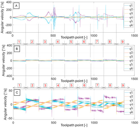
Figure 16.
Angular velocities of robotic axes (joints) along the toolpath ((A)—default, (B)—optimised, (C)—optimised with higher scale on y-axis, Numbers 1–9 in red indicate individual tool passes).
Subsequently, the robot’s power consumption was measured, with the default NC programme executed first. The power consumption characteristic (orange line in Figure 17) showed considerable spikes in power consumption, caused by the robot approaching singular positions. Such situations can occur at multiple points during five-axis machining.
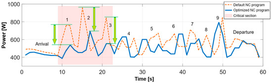
Figure 17.
Measured power consumption during robot movement using the default NC programme and optimised NC programme, with critical toolpath section highlighted by red box (Numbers 1–9 indicate individual tool passes, green arrows shows significant decrease of power consumption).
This was followed by executing the NC programme generated by the discretisation algorithm to perform the measurement. As shown by the blue line in Figure 17, the spikes in the power consumption characteristic were suppressed. This led to a reduction in the overall power consumption of the operation. As can also be observed, a higher peak in local power consumption appeared in the optimised NC programme compared to the default version, specifically in tool pass 4. Furthermore, in tool passes 4–9, a noticeable time shift in the power peaks was present. This shift resulted from the specific angular configurations of the robot joints in the optimised NC programme, differing from those in the default setup. A comparison of the measured data for the five-axis operation is presented in Table 6, showing a significant reduction of 7.5% in power consumption compared to the default NC programme.
Table 6.
Comparison of measured data for the entire toolpath of the five-axis operation.
Furthermore, the critical section highlighted by the red box in Figure 17 was also evaluated. This section showed the greatest improvement in electricity savings, approximately 20%, with average power consumption also decreasing by about 20%. A comparison of measured data for this critical section is presented in Table 7.
Table 7.
Measured values and comparison for the critical section of the five-axis operation toolpath.
It is therefore evident that the discretisation algorithm has a significant effect in tasks requiring the use of five-axis toolpaths for robot control, especially in situations where positions close to singularities occur. Such toolpath cases are applied in many manufacturing applications, such as operations with rotary tools (spindles), including machining, polishing and grinding, or with non-rotary tools (working heads), which may involve additive technologies (welding, large-format 3D printing, etc.), laser technologies, waterjet cutting, certain types of part manipulation tasks and so on. According to the type of end-effector, the possible range of limitation on the rotation angle of the effector around its own axis is determined. Therefore, the discretisation function has a broad spectrum of applications.
The proposed design of the discretisation algorithm, due to its simple implementation, is suitable for direct integration into the technological preparation of production processes using CAD/CAM systems, specifically as an additional function within the postprocessor. By enhancing user-friendliness, such implementation ensures efficient utilisation. To achieve greater benefits, the use of more advanced algorithms could be considered.
Therefore, future research could explore the implementation of genetic or generative approaches to optimise the selection of cutting conditions, particularly in the context of discrete value sets, as in the present case. Several methodologies—such as variational autoencoders (VAEs) for discrete data, generative adversarial networks (GANs) adapted for discrete spaces, genetic algorithms and reinforcement learning—could be considered, as discussed in [33,34,35,36].
4. Conclusions
This paper presented a novel approach for exploiting redundant degrees of freedom in six-axis robot applications for manufacturing operations. The proposed method is based on a simplified calculation of an energy consumption criterion for robotic manufacturing processes. This criterion is integrated into a discretisation algorithm that processes the toolpath and automatically selects the optimal rotation angle of the effector around its axis, such that the specific rotations of the robot’s individual axes (joints) minimise power consumption during the manufacturing operation. The algorithm searches for the optimal angle for each tool pass along the entire toolpath in cases of “zig,” “zag” or “zig-zag” operations, excluding any unused traversal sections of the toolpath.
Due to the algorithm’s simplicity, its implementation is straightforward and was incorporated as an additional function within the postprocessor when generating NC programmes from the CAM system for the robot. It was verified by measuring power consumption directly from the robot. The results indicate that the discretisation algorithm does not yield significant benefits for three-axis manufacturing operations. However, substantial energy savings were observed in multi-axis toolpath operations, with a 7.5% reduction in total energy consumption when using the NC programme generated by the proposed algorithm compared to the default NC programme obtained conventionally from the CAM system.
Consequently, the algorithm is applicable in various production applications, including operations performed by end-effectors with rotary tools (spindles), such as machining, polishing and grinding, as well as non-rotary tools (heads) involved in additive technologies (e.g., welding, large-format 3D printing), laser processing, waterjet cutting and certain part manipulation tasks. The presented solution offers an innovative approach that achieves significant power savings while maintaining user-friendliness, making it readily applicable to many robot-based manufacturing operations.
With regard to the practical implementation of the proposed optimisation method, it is essential to consider limitations related to potential collisions. A key concern is the possible collision between the end effector and the workpiece, which may occur due to the effector’s specific orientation around its axis. However, collision detection is a standard task for technologists working with CAM systems and is routinely incorporated into the NC programme preparation process, particularly in robotic applications. In practice, once a collision is detected, the technologist can select an alternative axis configuration from the ranked list of robot individual configurations generated by the optimisation (from least to most energy-intensive). While this step could be automated (since some CAM systems can generate collision detection reports), its reliability depends on the accuracy of the 3D kinematic models of the robot, end effector and any fixtures involved. In real-world scenarios, these may not exactly match the modelled geometry (especially with regard to the fixtures). Therefore, it remains advisable for the technologist to manually perform the final check in order to account for any potential discrepancies in the visualisation.
Future research may focus on the development of a user-friendly add-on for robot postprocessors, enabling the implementation and selection of various robot types from a predefined library. Such a tool would facilitate broader adoption of the proposed method among robot users. Additionally, further enhancement of the method could involve the variation of the redundant angle C along the process phase of the technological operation. This feature is currently not included due to its high computational complexity.
Author Contributions
P.V.: Conceptualisation, Methodology, Project Administration, Writing—Original Draft; S.P.: Software, Visualisation, Data Curation, Writing—Original Draft; T.K.: Methodology, Data Curation, Formal Analysis. All authors have read and agreed to the published version of the manuscript.
Funding
This work was created within the project National Centre of Competence in ENGINEERING (TN02000018), which is co-financed from the state budget by the Technology agency of the Czech Republic under the National Centre of Competence Programme. The authors would like to acknowledge also the support from European Structural and Investment Funds and the Operational Programme Research, Development and Education via the Ministry of Education, Youth and Sports of the Czech Republic, under the project CZ.02.1.01/0.0/0.0/16_026/ 0008432 Cluster 4.0—Methodology of System Integration. The authors would like to acknowledge usage of the RICAIP infrastructure for experimental part of the work.
Data Availability Statement
The original contributions presented in this study are included in the article. Further inquiries can be directed to the corresponding author.
Acknowledgments
The authors would like to acknowledge the usage of the RICAIP infrastructure for the experimental part of the work.
Conflicts of Interest
The authors declare that they have no known competing financial interests or personal relationships that could have appeared to influence the work reported in this paper.
Abbreviations
The following abbreviations are used in this manuscript:
| NC | Numerical Control |
| CAM | Computer-Aided Manufacturing |
| DOF | Degree of Freedom |
| K-K | Khalil–Kleinfinger |
| TCP | Tool Centre Point |
| DLL | Dynamic Link Libraries |
| MIG | Metal Inert Gas |
| MAG | Metal Active Gas |
References
- Gao, Y.; Qiu, T.; Song, C.; Ma, S.; Liu, Z.; Liang, Z.; Wang, X. Optimizing the performance of serial robots for milling tasks: A review. Robot. Comput.-Integr. Manuf. 2025, 94, 102977. [Google Scholar] [CrossRef]
- Brunete, A.; Gambao, E.; Koskinen, J.; Heikkilä, T.; Kaldestad, K.B.; Tyapin, I.; Hovland, G.; Surdilovic, D.; Hernando, M.; Bottero, A. Hard material small-batch industrial machining robot. Robot. Comput.-Integr. Manuf. 2018, 54, 185–199. [Google Scholar] [CrossRef]
- Wang, W.; Tian, W.; Liao, W.; Li, B.; Hu, J. Error compensation of industrial robot based on deep belief network and error similarity. Robot. Comput.-Integr. Manuf. 2022, 73, 102220. [Google Scholar] [CrossRef]
- Ozturk, E.; Barrios, A.; Sun, C.; Rajabi, S.; Munoa, J. Robotic assisted milling for increased productivity. CIRP Ann. 2018, 67, 427–430. [Google Scholar] [CrossRef]
- Zhang, Y.; Guo, P.; Huang, N.; Zhang, Y.; Zhu, L. A milling test-based coordinate calibration approach for the dual-robot mirror milling system with a measurement module. Robot. Comput.-Integr. Manuf. 2024, 89, 102749. [Google Scholar] [CrossRef]
- Wang, R.; Sun, Y. Chatter prediction for parallel mirror milling of thin-walled parts by dual-robot collaborative machining system. Robot. Comput.-Integr. Manuf. 2024, 88, 102715. [Google Scholar] [CrossRef]
- Yuan, L.; Sun, S.; Pan, Z.; Ding, D.; Gienke, O.; Li, W. Mode coupling chatter suppression for robotic machining using semi-active magnetorheological elastomers absorber. Mech. Syst. Signal Process. 2019, 117, 221–237. [Google Scholar] [CrossRef]
- Sun, L.; Zheng, K.; Liao, W.; Liu, J.; Feng, J.; Dong, S. Investigation on chatter stability of robotic rotary ultrasonic milling. Robot. Comput.-Integr. Manuf. 2020, 63, 101911. [Google Scholar] [CrossRef]
- Cordes, M.; Hintze, W.; Altintas, Y. Chatter stability in robotic milling. Robot. Comput.-Integr. Manuf. 2019, 55, 11–18. [Google Scholar] [CrossRef]
- Xin, S.; Peng, F.; Tang, X.; Yan, R.; Li, Z.; Wu, J. Research on the influence of robot structural mode on regenerative chatter in milling and analysis of stability boundary improvement domain. Int. J. Mach. Tools Manuf. 2022, 179, 103918. [Google Scholar] [CrossRef]
- Wu, J.; Peng, F.; Tang, X.; Yan, R.; Xin, S.; Mao, X. Characterization of milling robot mode shape and analysis of the weak parts causing end vibration. Measurement 2022, 203, 111934. [Google Scholar] [CrossRef]
- Busch, M.; Schnoes, F.; Elsharkawy, A.; Zaeh, M.F. Methodology for model-based uncertainty quantification of the vibrational properties of machining robots. Robot. Comput.-Integr. Manuf. 2022, 73, 102243. [Google Scholar] [CrossRef]
- Liu, Y.; Wang, L.; Yu, Y.; Zhang, J.; Shu, B. Optimization of redundant degree of freedom in robot milling considering chatter stability. Int. J. Adv. Manuf. Technol. 2022, 121, 8379–8394. [Google Scholar] [CrossRef]
- Liu, J.; Zhao, Y.; Niu, Y.; Cao, J.; Zhang, L.; Zhao, Y. Optimization of Redundant Degrees of Freedom in Robotic Flat-End Milling Based on Dynamic Response. Appl. Sci. 2024, 14, 1877. [Google Scholar] [CrossRef]
- Zhu, W.; Qu, W.; Cao, L.; Yang, D.; Ke, Y. An off-line programming system for robotic drilling in aerospace manufacturing. Int. J. Adv. Manuf. Technol. 2013, 68, 2535–2545. [Google Scholar] [CrossRef]
- Chen, C.; Peng, F.; Yan, R.; Li, Y.; Wei, D.; Fan, Z.; Tang, X.; Zhu, Z. Stiffness performance index based posture and feed orientation optimization in robotic milling process. Robot. Comput.-Integr. Manuf. 2019, 55, 29–40. [Google Scholar] [CrossRef]
- Xiong, G.; Ding, Y.; Zhu, L. Stiffness-based Pose Optimization of an Industrial Robot for Five-axis Milling. Robot. Comput.-Integr. Manuf. 2019, 55, 19–28. [Google Scholar] [CrossRef]
- Schneider, U.; Verl, A.W.; Posada, J.R.D. Automatic Pose Optimizaion for Robotic Processes. In Proceedings of the 2015 IEEE International Conference on Robotics and Automation (ICRA), Seattle, WA, USA, 26–30 May 2015; pp. 2054–2059. [Google Scholar] [CrossRef]
- Guo, Y.; Dong, H.; Ke, Y. Stiffness-oriented posture optimizaion in robotic machining applications. Robot. Comput.-Integr. Manuf. 2015, 35, 69–76. [Google Scholar] [CrossRef]
- Kratěna, T.; Vavruška, P.; Švéda, J.; Zeman, P. Workpiece position optimisation in robotic multi-axis machining. Results Eng. 2025, 27, 106421. [Google Scholar] [CrossRef]
- Cvitanic, T.; Nguyen, V.; Melkote, S.N. Pose optimization in robotic machining using static and dynamic stiffness models. Robot. Comput.-Integr. Manuf. 2020, 66, 101992. [Google Scholar] [CrossRef]
- Ratiu, M.; Prichici, M.A. Industrial robot trajectory optimizaion—A review. MATEC Web Conf. 2017, 126, 02005. [Google Scholar] [CrossRef]
- Erdős, G.; Kovács, A.; Váncza, J. Optimized joint motion planning for redundant industrial robots. CIRP Ann. 2016, 65, 451–454. [Google Scholar] [CrossRef]
- Flacco, F.; De Luca, A. Discrete-Time Velocity Contrrol of Reduindant Robots with Acceleration/Torque Optimizaion Properties. In Proceedings of the 2014 IEEE International Conference on Robotics and Automation (ICRA), Hong Kong, China, 31 May–7 June 2014; pp. 5139–5144. [Google Scholar] [CrossRef]
- Garcia, R.R.; Bittencourt, A.C.; Villani, E. Relevant factors for the energy consumption of industrial robots. J. Braz. Soc. Mech. Sci. Eng. 2018, 40, 464. [Google Scholar] [CrossRef]
- Khalaf, P.; Richter, H. On Global, Closed-Form Solutions to Parametric Optimization Problems for Robots With Energy Regeneration. J. Dyn. Syst. Meas. Control 2017, 140, 031003. [Google Scholar] [CrossRef]
- Soori, M.; Arezoo, B.; Dastres, R. Optimization of energy consumption in industrial robots, a review. Cogn. Robot. 2023, 3, 142–157. [Google Scholar] [CrossRef]
- Feng, Y.; Ji, Z.; Gao, Y.; Zheng, H.; Tan, J. An energy-saving optimization method for cyclic pick-and-place tasks based on flexible joint configurations. Robot. Comput.-Integr. Manuf. 2021, 67, 102037. [Google Scholar] [CrossRef]
- Zhou, J.; Yi, H.; Cao, H.; Jiang, P.; Zhang, C.; Ge, W. Structural decomposition-based energy consumption modeling of robot laser processing systems and energy-efficient analysis. Robot. Comput.-Integr. Manuf. 2022, 76, 102327. [Google Scholar] [CrossRef]
- Zhang, M.; Yan, J. A data-driven method for optimizing the energy consumption of industrial robots. J. Clean. Prod. 2021, 285, 124862. [Google Scholar] [CrossRef]
- Pastras, G.; Fysikopoulos, A.; Chryssolouris, G. A theoretical investigation on the potential energy savings by optimization of the robotic motion profiles. Robot. Comput.-Integr. Manuf. 2019, 58, 55–68. [Google Scholar] [CrossRef]
- Ruzarovsky, R.; Horak, T.; Bocak, R.; Csekei, M.; Zelník, R. Integrating Energy and Time Efficiency in Robotic Manufacturing Cell Design: A Methodology for Optimizing Workplace Layout. Machines 2025, 13, 38. [Google Scholar] [CrossRef]
- Agrawal, R.K.; Pratihar, D.K.; Roy Choudhury, A. Optimization of CNC isoscallop free form surface machining using a genetic algorithm. Int. J. Mach. Tools Manuf. 2006, 46, 811–819. [Google Scholar] [CrossRef]
- Fountas, N.A.; Stergiou, C.I.; Majstorović, V.D.; Vaxevanidis, N.M. Intelligent Optimization for Sculptured Surface CNC Tool-paths. Procedia CIRP 2016, 55, 140–145. [Google Scholar] [CrossRef]
- Rezaei, S.; Cornelius, A.; Karandikar, J.; Schmitz, T.; Khojandi, A. Using GANs to predict milling stability from limited data. J. Intell. Manuf. 2024, 36, 1201–1235. [Google Scholar] [CrossRef]
- Yildiz, A.R.; Ozturk, F. Hybrid enhanced genetic algorithm to select optimal machining parameters in turning operation. Proc. Inst. Mech. Eng. Part B J. Eng. Manuf. 2006, 220, 2041–2053. [Google Scholar] [CrossRef]
Disclaimer/Publisher’s Note: The statements, opinions and data contained in all publications are solely those of the individual author(s) and contributor(s) and not of MDPI and/or the editor(s). MDPI and/or the editor(s) disclaim responsibility for any injury to people or property resulting from any ideas, methods, instructions or products referred to in the content. |
© 2025 by the authors. Licensee MDPI, Basel, Switzerland. This article is an open access article distributed under the terms and conditions of the Creative Commons Attribution (CC BY) license (https://creativecommons.org/licenses/by/4.0/).