ROS-Based Autonomous Driving System with Enhanced Path Planning Node Validated in Chicane Scenarios

Abstract

In modern vehicles, Autonomous Driving Systems (ADSs) are designed to operate partially or fully without human intervention. The ADS pipeline comprises multiple layers, including sensors, perception, localization, mapping, path planning, and control. The Robot Operating System (ROS) is a widely adopted framework that supports the modular development and integration of these layers. Among them, the path-planning and control layers remain particularly challenging due to several limitations. Classical path planners often struggle with non-smooth trajectories and high computational demands. Meta-heuristic optimization algorithms have demonstrated strong theoretical potential in path planning; however, they are rarely implemented in real-time ROS-based systems due to integration challenges. Similarly, traditional PID controllers require manual tuning and are unable to adapt to system disturbances. This paper proposes a ROS-based ADS architecture composed of eight integrated nodes, designed to address these limitations. The path-planning node leverages a meta-heuristic optimization framework with a cost function that evaluates path feasibility using occupancy grids from the Hector SLAM and obstacle clusters detected through the DBSCAN algorithm. A dynamic goal-allocation strategy is introduced based on the LiDAR range and spatial boundaries to enhance planning flexibility. In the control layer, a modified Pure Pursuit algorithm is employed to translate target positions into velocity commands based on the drift angle. Additionally, an adaptive PID controller is tuned in real time using the Differential Evolution (DE) algorithm, ensuring robust speed regulation in the presence of external disturbances. The proposed system is practically validated on a four-wheel differential drive robot across six scenarios. Experimental results demonstrate that the proposed planner significantly outperforms state-of-the-art methods, ranking first in the Friedman test with a significance level less than 0.05, confirming the effectiveness of the proposed architecture.

1. Introduction

Autonomous Driving Systems (ADSs) are vehicles equipped with advanced technology that can partially or fully operate without human intervention. The early vision of autonomous driving can be traced to the early 20th century by Norman Bel Geddes in 1939 at the New York World’s Fair [1]. In 2004, DARPA Challenges introduced a competition for the design of ADSs. These competitions encourage teams worldwide to design self-driving cars [2]. The evolving technologies in control systems, sensors, and artificial intelligence self-driving improved the design and implementation of the ADS and shaped the modern ADS industry.

1.1. Autonomous Driving System (ADS)

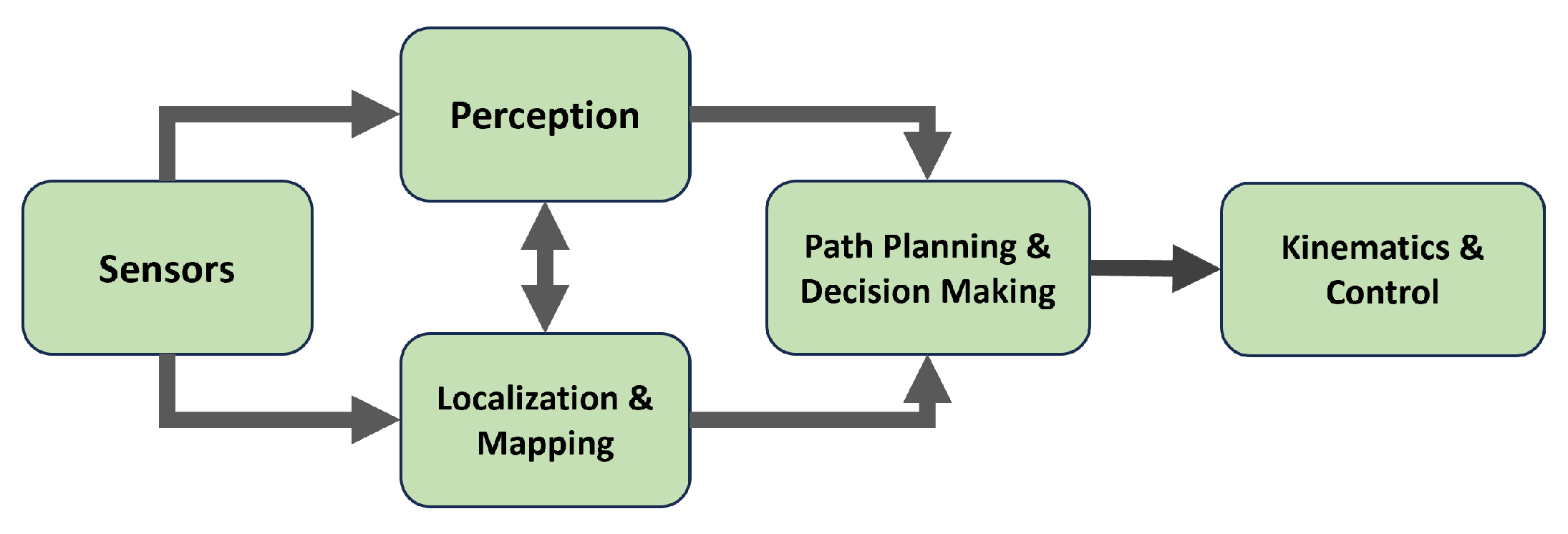
The pipeline of the ADS consists of five stages, as seen in Figure 1. It starts with sensors that collect data about the vehicle and its surroundings, such as LiDAR, cameras, encoders, and IMU sensors. In the perception stage, the data from cameras are used by computer vision algorithms to recognize the objects around the car, such as traffic lights, road signs, and lanes [3]. In the localization and mapping stage, the data from sensors such as LiDARs, encoders, GPS, and IMU sensors are used to locate the current position and orientation of the vehicle and create a map of the surrounding environment [4]. The information from the perception and mapping layers is fed to the path-planning and decision-making stage to determine the next position that the car should take, avoiding obstacles and obeying traffic rules [5].

Finally, the location generated by the path-planning stage is converted to motor control action based on the car’s mechanism. Different car architectures are based on steering mechanisms, such as two-wheel differential drive, four-wheel differential drive, and Ackerman steering [6]. In the final layer, the kinematics equations are implemented to convert the desired position into the corresponding speed and steering angles that should be applied to the motors to reach the goal [7].

1.2. Overview of the State-of-the-Art and Research Gap

The Robot Operating System (ROS) is widely adopted as a core development framework for autonomous driving systems. Most ADS prototypes utilize ROS for managing sensor data, localization, path planning, and actuator control, providing a practical foundation for developing and testing autonomous navigation systems [8].

The perception and mapping layers in autonomous driving systems are well established and have been extensively studied. In the perception layer, cameras are commonly used to capture visual data. These data are then processed using deep learning techniques, such as Convolutional Neural Networks (CNNs), for object detection and scene understanding [9].

For mapping and localization, various sensors are integrated with SLAM (Simultaneous Localization and Mapping) algorithms to construct maps and estimate the vehicle’s position. Among SLAM variants, camera-based SLAM offers rich semantic information but lacks depth accuracy and is computationally intensive [10]. Radar-based SLAM performs well in adverse weather conditions but suffers from lower resolution [11]. LiDAR-based SLAM provides high spatial accuracy and reliable depth information, making it a balanced and widely adopted solution [12]. Accordingly, this work employs LiDAR-SLAM as the mapping framework.

The control layer in the ADS ensures the vehicle accurately follows planned trajectories by minimizing the error between the desired and actual states. The most widely used method is the Proportional–Integral–Derivative (PID) controller due to its simplicity, robustness, and low computational cost [13]. However, PID performance heavily depends on proper gain tuning, which is traditionally performed using offline methods such as the Ziegler–Nichols (ZN) technique [14]. These static gains are platform-specific and often require manual re-tuning when system dynamics change or external disturbances occur. While ROS provides packages for PID integration, they require predefined gains and do not support real-time adaptation [15]. This limitation highlights a significant gap in the existing ROS ecosystem, where there is no built-in mechanism for adaptive, feedback-driven PID tuning that can adjust gains dynamically during runtime in response to changing conditions.

Path planning remains one of the most challenging components of the ADS, as it must generate collision-free, dynamically feasible trajectories in real time [16]. Classical algorithms offer varied trade-offs. The A* algorithm, a grid-based method, guarantees optimality in structured environments but suffers from slow execution and sharp paths in dense maps [17]. Rapidly Exploring Random Tree (RRT), a sampling-based method, improves speed compared to A* but generates non-optimal, sharp trajectories [18]. The Dynamic Window Approach (DWA), a trajectory-based method, considers vehicle dynamics and produces smooth local paths. However, it incurs a high computational cost and may become stuck in local minima [19]. The Timed Elastic Band (TEB), an optimization-based trajectory planner, achieves smoother paths; however, it remains sensitive to tuning and is computationally expensive in complex environments.

In contrast, meta-heuristic algorithms such as Particle Swarm Optimization (PSO) and Differential Evolution (DE) offer flexible, gradient-free search capabilities that perform well in global path-optimization problems [20,21]. However, these techniques are typically applied in simulation, often with MATLAB or Python (any version), and are not integrated into practical ROS-based frameworks. This gap highlights the absence of a unified, ROS-based path planner that can adopt meta-heuristic optimization and real-time feedback.

1.3. Contributions

To address the identified limitations in control and planning layers, this study proposes a modular and extensible ROS-based framework designed for practical deployment on ADS platforms. The proposed approach enhances the system’s adaptability and performance in complex environments by embedding a feedback-driven PID tuning mechanism and a meta-heuristic-based path planner within a modular architecture. The key contributions of this research are summarized below.

• A modular ROS-based autonomous driving system is proposed, consisting of eight integrated nodes, including two novel nodes: an RDE-based path-planning node and an adaptive control node.
• The path-planning node employs a Differential Evolution (RDE) optimizer with dynamic goal allocation based on LiDAR range and search space boundaries. Moreover, a custom cost function evaluates path feasibility by incorporating penalties based on Hector-SLAM occupancy grids and DBSCAN-identified obstacle clusters.
• The control node integrates a DE-based adaptive PID controller for speed regulation and a modified Pure Pursuit algorithm with drift compensation to convert planned paths into motor commands.
• Experimental validation on a 4WD robot across six navigation scenarios demonstrates that the proposed system outperforms A*, RRT, DWA, and A*TEB, ranking first in the Friedman test with a significance level of $p<0.05$.

1.4. Paper Organization

The rest of the paper is organized as follows: Section 2 reviews the state-of-the-art in ADSs and path planning. Section 3 presents a comparative study of 15 meta-heuristic algorithms to select the optimal optimizer. Section 4 details the proposed ROS-based ADS architecture and its eight integrated nodes. Section 5 describes the hardware implementation of the 4WD robot used for validation. Section 6 evaluates the PID control performance using DE-based tuning. Section 7 validates the whole system across six navigation scenarios. Section 8 provides a statistical analysis of the results. Section 9 discusses the computational complexity of the system. Section 10 outlines deployment considerations for outdoor and dynamic environments. Finally, Section 11 concludes the study and suggests directions for future work.

2. Related Work

Autonomous navigation systems rely on multiple interdependent modules including path planning and control. Numerous studies have proposed classical and modern techniques for path planning and trajectory optimization. In this section, we review the most relevant literature on classical path-planning algorithms, meta-heuristic optimization techniques, and control approaches in autonomous driving, with a focus on the limitations of existing solutions in practical ROS-based systems.

2.1. Control Algorithms and PID Tuning

The control algorithm manages how an autonomous system minimizes the error between the desired and actual output in a closed-loop system. Classic PID controllers are the most widely used approach in industry and robotics, covering more than 95% of control systems. It is used due to its simplicity, low computational cost, and effective performance [13].

A PID controller includes three components: proportional, integral, and derivative terms, which must be tuned appropriately for each platform. The most popular tuning approach is the Ziegler–Nichols (ZN) method [14]. However, ZN provides platform-dependent static gains, which often require manual re-tuning if system conditions change or disturbances occur.

In ROS, although there is no native universal PID node, PID functionality is available through the ‘control_toolbox::Pid’ library, which is used by controllers like ‘ros_control’ [15]. However, these require static, YAML-defined gains and lack real-time tuning or auto-adaptive capabilities. This issue presents a clear gap in ROS for online PID tuning mechanisms that can adjust gains in response to sensor feedback or platform changes, especially in systems such as autonomous driving platforms.

2.2. Path-Planning Algorithms

Path planning enables autonomous systems to compute safe and efficient trajectories from start to goal positions while avoiding obstacles. This section reviews key algorithms applied in recent literature.

2.2.1. A* Algorithm

A* is a widely used graph-based algorithm that converts the environment into a grid and uses a heuristic cost function to determine the shortest path. Its deterministic nature make it attractive for structured static environments. Several studies have deployed A* in diverse applications.

Yijing et al. [22] implemented A* for local path planning, but it lacks statistical benchmarking. Udomsil et al. [23] integrated A* with collision-detection mechanisms for static motion planning. However, their work did not include comparisons with alternative algorithms. Zhong et al. [24] employed A* for real-time trajectory planning, but relied heavily on unoptimized parameter settings, which limited generalizability.

Li et al. [25] applied A* to guide automated guided vehicles (AGVs), while Zhang et al. [26] introduced adaptive cost functions to improve AGV pathfinding. Thoresen et al. [27] validated A* on real terrain with unmanned ground vehicles (UGVs) using traversability analysis. Liu and Zhang [28] further applied A* in idle traffic to optimize fuel consumption, though their method lacked real-world testing.

Despite these varied applications, A* is limited in scalability and flexibility. It performs well in simple environments but suffers from computational inefficiency in dense maps. It often produces jagged or abrupt trajectories that require post-processing [29]. In ROS-based implementations, A* is used as a global planner [30]. This usage necessitates integration with a local planner (e.g., DWA or TEB) to generate feasible paths suitable for real-world navigation. This dependency introduces further complexity, particularly in unknown environments.

2.2.2. Rapidly Exploring Random Tree (RRT)

RRT is a sampling-based algorithm that incrementally builds a tree by randomly sampling points in the search space and connecting them to the nearest nodes, expanding the tree towards unexplored areas. Wang et al. [31] applied RRT to autonomous vehicles and reported smoother and faster paths than A*, but their work lacked thorough statistical analysis.

Chen et al. [32] employed RRT* for obstacle-dense environments, achieving collision-free paths, but at a high computational cost, and without comparison to competing methods. Hu et al. applied an RRT-based framework for motion planning in a wheeled robot under kinodynamic constraints [33]. Niu et al. [34] implemented RRT in a ROS-based platform for intelligent vehicles. Shi et al. [35] applied B-spline interpolation to smooth RRT-generated paths for unmanned vehicles.

Further extensions include Chen et al. [36], who reduced the search space using constrained sampling. Yang and Yao focused on path pruning and smoothing [37]. Zhang et al. [38] introduced adaptive directional sampling but found the algorithm computationally intensive. Mao et al. [39] improved RRT with an elliptical sampling domain to lower path costs.

RRT offers faster solutions than A* without requiring an explicit map. However, it also generates sharp paths, making them less suitable for practical applications without the use of interpolation techniques. It cannot guarantee the shortest path, and its performance deteriorates as obstacle density increases. Therefore, real-time ROS implementations remain limited due to the computational overhead and the lack of general-purpose path planning without coupling with another method.

2.2.3. Dynamic Window Approach (DWA)

The Dynamic Window Approach (DWA) is a trajectory-based path-planning algorithm that generates motion commands by sampling velocity pairs within the robot’s dynamic constraints. It is one of the most widely adopted local planners in ROS-based systems [40]. Zhang et al. [41] applied the DWA to mobile robots, validating it in a two-wheel differential drive simulation environment on ROS. Liu et al. [42] implemented DWA for a smart four-wheel robot, while Hua et al. [43] enhanced DWA with an adaptive objective function. Kobayashi et al. [19] demonstrated a basic DWA planner in a simple obstacle setting with a differential robot.

Although DWA considers vehicle kinematics and produces smooth short-term plans, DWA suffers from a high computational cost. Its computational complexity grows cubically with the number of velocity samples ($\mathcal{O}\left(n^3\right)$), making it inefficient in cluttered or complex environments [44]. Moreover, DWA-generated paths tend to include an excessive number of waypoints, which increases execution time and degrades responsiveness. In ROS, DWA is typically used in conjunction with a global planner, such as A*, which limits its standalone applicability and generalizability.

2.2.4. Timed Elastic Band (TEB)

The Timed Elastic Band (TEB) algorithm formulates local planning as a trajectory-optimization problem over a time-parameterized sequence of poses (elastic band). It is widely adopted in ROS as a standard local planner within the ‘move_base’ framework [45].

Wu et al. demonstrated its integration and visualization in a ROS environment for local navigation tasks [46]. Dang et al. applied A*-TEB in a 4WD robotic platform for static map navigation [47], while Kulathunga et al. validated a similar architecture on an Agilex Hunter 2.0 platform within ROS [48]. Xi et al. extended TEB for unstructured terrains using a 4-wheel robot [49], and Turnip et al. employed it for medical robotic applications, reporting improved performance over DWA in a ROS setup [50].

TEB offers advantages over the DWA by optimizing complete trajectories rather than sampling velocity pairs, resulting in smoother paths. However, it suffers from high computational overhead in complex environments. Additionally, TEB’s performance is highly sensitive to parameter tuning, which must be manually adjusted for each robot platform or scenario.

2.3. Meta-Heuristic Optimization Algorithms in Path Planning

Meta-heuristic optimization algorithms are high-level search techniques inspired by natural and biological processes. They have proven particularly effective in solving complex and NP-hard problems due to their flexibility and ability to escape local optima without requiring gradient information. In the context of robotics and autonomous navigation, these algorithms have been widely applied to the path-planning problem, where the goal is to compute collision-free paths in environments with multiple obstacles [51].

Evolutionary-based algorithms include Genetic Algorithm (GA) [52], which evolves solutions through selection, crossover, and mutation. Differential Evolution (DE) [21] is recognized for its simple and efficient mutation and crossover schemes. Covariance Matrix Adaptation Evolution Strategy (CMA-ES) [53] is also a robust evolutionary algorithm that adapts the covariance matrix of its search distribution to guide the optimization process.

Swarm-based algorithms are inspired by the collective behavior of animals. Particle Swarm Optimization (PSO) [20,21] is based on the movement of bird flocks. The Artificial Bee Colony (ABC) [52] simulates the foraging behavior of bees, while the Grey Wolf Optimizer (GWO) [54] models the social hierarchy and hunting mechanism of wolves. The Artificial Hummingbird Algorithm (AHA) [55] and Moth Flame Optimization (MFO) [56] also fall into this category.

Nature-inspired algorithms imitate physical or ecological phenomena. Thermal Exchange Optimization (TEO) [57] is based on thermodynamic heat transfer. The Generalized Normal Distribution Optimization (GNDO) [58] uses statistical properties of normal distributions. The Firefly Algorithm (FA) [52] models firefly attraction behavior, while Beetle Antennae Search (BAS) [59,60] is based on beetle foraging. The Liver Cancer Algorithm (LCA) [61] is inspired by the mutation behavior of liver cancer cells.

Despite the promising performance of these algorithms in path planning compared to traditional methods, they remain limited to simulation environments and lack direct integration within the ROS ecosystem. They are often implemented using MATLAB or Python and evaluated on simulated benchmarks or predefined obstacle maps. Moreover, current ROS planning frameworks, including ‘move_base’, are not natively designed to support general-purpose meta-heuristic optimization in dynamic, SLAM-based environments. This lack of practical integration highlights a critical research gap, motivating the development of a ROS-based path-planning node that supports meta-heuristic optimization and enables real-time operation in dynamic environments, as detailed in the following sections.

3. Benchmark-Driven Meta-Heuristic Optimizer Selection

Before explaining the ROS system design, this section focuses on selecting the most suitable optimization algorithm for the forthcoming Path-Planning and Control nodes. This section, therefore, benchmarks fifteen widely used meta-heuristic algorithms on the CEC2020 test suite, evaluating each in terms of solution quality and execution time. By combining statistical accuracy metrics with normalized run-time scores, we isolate the single optimizer that delivers the best accuracy–speed trade-off; this data-driven choice is then adopted throughout the remainder of the paper.

3.1. Experimental Setup

The following 15 algorithms are included in the comparison: GA, PSO, TEO, GNDO, SA, ABC, GWO, AHA, BAS, FA, MFO, LCA, HHO, CMAES, and DE. The parameter settings for these algorithms are set as recommended by their original work and are summarized in Table 1. Each algorithm is executed independently for 30 runs per benchmark function to ensure statistically reliable results.

The CEC2020 benchmark suite is employed, consisting of 10 functions: one unimodal (F1), three multimodal (F2–F4), three hybrid (F5–F7), and three composition functions (F8–F10). Each function is evaluated in two dimensions (10D and 20D), resulting in a total of 20 distinct test cases [62]. All functions use a fixed search range of [−100, 100], and each algorithm is terminated either upon reaching a solution with an error below ${10}^{-8}$ or the maximum number of function evaluations (MaxFEs) (200,000 for 10D, 500,000 for 20D), whichever came first.

Table 1. Parameter settings for all the meta-heuristic optimization algorithms.

Algorithm	Parameters
GA [52]	$NP=30$, $P_c$ = 0.8, tournament size = 3
	$P_m$ = 0.3, $\mu$ = 0.02
PSO [20,21]	$NP=30$, $c_1$ = 1, $c_2$ = 1, w = 0.3
TEO [57]	$NP=30$, $p=0.3$, $STO=5$
GNDO [58]	$NP=30$
SA [63,64]	max No. of sub-iteration = 20, No. of neighbors per individual = 5,
	$NP=30$, $\alpha$ = 0.99, $T_0$ = 0.1, mutation rate $\mu$ = 0.5
ABC [52]	$NP=30$, abandon limit = $0.6$ * D * NP,
	No. of onlooker bees = NP, a = 1
GWO [54]	$NP=30$, a: linearly decreases from 2 to 0
AHA [55]	$NP=30$, Migration Coef. = $2\ast NP$
BAS [59]	$NP=30$, $d^1$ = 2, ${\eta }_d$ = 0.95, $d_0$ = 0.01
	${\delta }^1$ = 0.5, ${\eta }_{\delta }$ = 0.95, ${\delta }_0$ = 0.00
FA [52]	m = 2, mutation range = 0.05 * ( ub − lb), $\gamma$ = 1,
	$NP=30$, ${\beta }_0$ = 2, $\alpha$ = 0.2, damping ratio = 0.98
MFO [56]	$NP=30$, a: linearly decreases from −2 to −1, b = 1
LCA [61]	$NP=30$
HHO [20]	$NP=30$, escaping energy: randomly varies between [−2, 2]
CMAES [53]	$C_c$ = ${\displaystyle \frac{4}{D+4}}$, $c_{cov}$ = ${\displaystyle \frac{2}{{(D+\sqrt{2})}^2}}$
	$NP=30$, $\mu$ = $NP/2$, $d_{\sigma }$ = $c_{\sigma }^{-1}+1$
DE [21]	$NP=30$, F = 0.5, $CR$ = 0.5

Table 1. Parameter settings for all the meta-heuristic optimization algorithms.

Algorithm	Parameters
GA [52]	$NP=30$, $P_c$ = 0.8, tournament size = 3
	$P_m$ = 0.3, $\mu$ = 0.02
PSO [20,21]	$NP=30$, $c_1$ = 1, $c_2$ = 1, w = 0.3
TEO [57]	$NP=30$, $p=0.3$, $STO=5$
GNDO [58]	$NP=30$
SA [63,64]	max No. of sub-iteration = 20, No. of neighbors per individual = 5,
	$NP=30$, $\alpha$ = 0.99, $T_0$ = 0.1, mutation rate $\mu$ = 0.5
ABC [52]	$NP=30$, abandon limit = $0.6$ * D * NP,
	No. of onlooker bees = NP, a = 1
GWO [54]	$NP=30$, a: linearly decreases from 2 to 0
AHA [55]	$NP=30$, Migration Coef. = $2\ast NP$
BAS [59]	$NP=30$, $d^1$ = 2, ${\eta }_d$ = 0.95, $d_0$ = 0.01
	${\delta }^1$ = 0.5, ${\eta }_{\delta }$ = 0.95, ${\delta }_0$ = 0.00
FA [52]	m = 2, mutation range = 0.05 * ( ub − lb), $\gamma$ = 1,
	$NP=30$, ${\beta }_0$ = 2, $\alpha$ = 0.2, damping ratio = 0.98
MFO [56]	$NP=30$, a: linearly decreases from −2 to −1, b = 1
LCA [61]	$NP=30$
HHO [20]	$NP=30$, escaping energy: randomly varies between [−2, 2]
CMAES [53]	$C_c$ = ${\displaystyle \frac{4}{D+4}}$, $c_{cov}$ = ${\displaystyle \frac{2}{{(D+\sqrt{2})}^2}}$
	$NP=30$, $\mu$ = $NP/2$, $d_{\sigma }$ = $c_{\sigma }^{-1}+1$
DE [21]	$NP=30$, F = 0.5, $CR$ = 0.5

3.2. Statistical Evaluation Framework

The following performance metrics are recorded across all runs: median, mean, standard deviation (SD), best, and worst fitness values. Friedman test is applied to statistically evaluate the comparative performance of all algorithms across multiple benchmark functions (or scenarios). It is a non-parametric statistical test suitable for analyzing repeated measures or matched groups when parametric assumptions (e.g., normality) cannot be guaranteed.

Specifically, it ranks each algorithm based on its median error for every function (with rank 1 assigned to the best performance). The total rank for each algorithm $R_m$ is computed, where a lower rank indicates better overall performance. Then, the total rank $R_m$ is used to calculate the Friedman statistic $F_r$ as in Equation (1). Here, n is the number of functions (or scenarios), k is the number of algorithms, and $R_m$ is the sum of ranks for algorithm m.

$$F_r={\displaystyle \frac{12}{nk(k+1)}}\sum _{m=1}^k{R}_m^2-3n(k+1),$$

(1)

The resulting $F_r$ is then used to compute the p-value via the chi-square distribution with $k-1$ degrees of freedom. If $p<0.05$, we reject the null hypothesis, confirming that at least one algorithm performs significantly better than others. Detailed methodology and justification for using the Friedman test in multi-algorithm benchmarking are provided in [65,66].

In addition, the Wilcoxon Signed-Rank test is applied to perform pairwise comparisons between the DE algorithm and each of the other algorithms. This test evaluates whether the differences in performance are statistically significant. For each comparison, a ‘+’ indicates the number of functions in which the DE performed better (lower median error), ‘=’ indicates no significant difference, and ‘−’ indicates the competitor performed better. These analyses enable a rigorous selection of the most effective optimization algorithm for the proposed ROS-based autonomous driving system [65,67].

3.3. Statistical Analysis Results

The error metrics for all algorithms are presented in Appendix A (

Table A1. The best, worst, mean, median, SD results for the error metric for all meta-heuristic optimization algorithms, CEC2020 (F1–F10).

Fun	Alg.	10D					20D
No.	Name	Best	Worst	Median	Mean	SD	Best	Worst	Median	Mean	SD
F1	GA	1.4974 × ${10}^4$	1.7788 × ${10}^6$	3.6617 × ${10}^5$	5.0509 × ${10}^5$	4.3654 × ${10}^5$	1.2426 × ${10}^4$	2.6591 × ${10}^5$	5.3753 × ${10}^4$	7.4397 × ${10}^4$	6.4180 × ${10}^4$
	PSO	1.4168 × ${10}^6$	2.0380 × ${10}^9$	3.0350 × ${10}^8$	5.8239 × ${10}^8$	6.1165 × ${10}^8$	2.1809 × ${10}^9$	1.5419 × ${10}^{10}$	6.5854 × ${10}^9$	7.5710 × ${10}^9$	3.5970 × ${10}^9$
	TEO	1.1793 × ${10}^4$	8.7009 × ${10}^4$	2.3377 × ${10}^4$	4.0459 × ${10}^4$	2.8956 × ${10}^4$	1.9895 × ${10}^4$	1.2542 × ${10}^5$	9.8042 × ${10}^4$	8.6402 × ${10}^4$	3.2579 × ${10}^4$
	GNDO	3.5706	5.4951 × ${10}^3$	3.6748 × ${10}^2$	6.2313 × ${10}^2$	1.0436 × ${10}^3$	1.6474 × ${10}^{-6}$	9.7521 × ${10}^3$	4.3134 × ${10}^{-4}$	5.7523 × ${10}^2$	1.7676 × ${10}^3$
	SA	1.4496 × ${10}^6$	8.0358 × ${10}^6$	4.0704 × ${10}^6$	4.2385 × ${10}^6$	1.8020 × ${10}^6$	6.5182 × ${10}^5$	2.3992 × ${10}^6$	1.6167 × ${10}^6$	1.5951 × ${10}^6$	4.7568 × ${10}^5$
	ABC	2.2673 × 10	2.6460 × ${10}^3$	3.1767 × ${10}^2$	6.2372 × ${10}^2$	6.7841 × ${10}^2$	9.4640	1.1106 × ${10}^4$	2.0601 × ${10}^3$	2.8874 × ${10}^3$	2.7787 × ${10}^3$
	GWO	3.3673 × ${10}^2$	4.8782 × ${10}^8$	1.1451 × ${10}^4$	4.2925 × ${10}^7$	1.2103 × ${10}^8$	1.9767 × ${10}^2$	3.0740 × ${10}^9$	4.6268 × ${10}^8$	6.9956 × ${10}^8$	8.5131 × ${10}^8$
	AHA	1.3347	3.4245 × ${10}^3$	1.6803 × ${10}^3$	1.4297 × ${10}^3$	1.0617 × ${10}^3$	1.9126 × 10	4.7895 × ${10}^3$	1.5288 × ${10}^3$	1.7714 × ${10}^3$	1.9357 × ${10}^3$
	BAS	8.5458 × ${10}^9$	3.8408 × ${10}^{10}$	2.0401 × ${10}^{10}$	2.2467 × ${10}^{10}$	7.5480 × ${10}^9$	3.8225 × ${10}^{10}$	8.6432 × ${10}^{10}$	6.3699 × ${10}^{10}$	6.4602 × ${10}^{10}$	1.1161 × ${10}^{10}$
	FA	8.7940 × ${10}^{-1}$	5.8425 × ${10}^3$	1.4874 × ${10}^3$	2.0079 × ${10}^3$	1.9840 × ${10}^3$	4.4123	1.1691 × ${10}^4$	1.8836 × ${10}^3$	3.0924 × ${10}^3$	3.5731 × ${10}^3$
	MFO	1.5474	1.6049 × ${10}^9$	5.5320 × ${10}^3$	1.9685 × ${10}^8$	4.9533 × ${10}^8$	1.2092 × ${10}^4$	1.6428 × ${10}^{10}$	1.7118 × ${10}^9$	2.7251 × ${10}^9$	3.3182 × ${10}^9$
	LCA	9.0536 × ${10}^9$	2.7883 × ${10}^{10}$	2.1343 × ${10}^{10}$	1.8992 × ${10}^{10}$	6.9087 × ${10}^9$	4.2757 × ${10}^{10}$	4.7895 × ${10}^{10}$	4.5530 × ${10}^{10}$	4.5529 × ${10}^{10}$	1.9365 × ${10}^9$
	HHO	1.1640 × ${10}^7$	8.4877 × ${10}^8$	1.0479 × ${10}^8$	1.8747 × ${10}^8$	2.0781 × ${10}^8$	2.4371 × ${10}^7$	4.9665 × ${10}^8$	1.5918 × ${10}^8$	1.7041 × ${10}^8$	1.0456 × ${10}^8$
	CMAES	1.6829 × ${10}^3$	8.4241 × ${10}^9$	4.3266 × ${10}^9$	4.0683 × ${10}^9$	1.9841 × ${10}^9$	2.1323 × ${10}^2$	2.1728 × ${10}^{10}$	9.8212 × ${10}^9$	8.4589 × ${10}^9$	7.6954 × ${10}^9$
	DE	0.0000	0.0000	0.0000	0.0000	0.0000	0.0000	0.0000	0.0000	0.0000	0.0000
F2	GA	1.9127 × 10	8.2353 × ${10}^2$	3.5663 × ${10}^2$	3.8877 × ${10}^2$	2.0957 × ${10}^2$	1.1192 × 10	7.6484 × ${10}^2$	4.0814 × ${10}^2$	4.1054 × ${10}^2$	2.1424 × ${10}^2$
	PSO	2.4555 × ${10}^2$	1.4602 × ${10}^3$	1.0420 × ${10}^3$	1.0210 × ${10}^3$	3.2130 × ${10}^2$	1.3760 × ${10}^3$	3.1143 × ${10}^3$	2.3544 × ${10}^3$	2.2551 × ${10}^3$	5.0741 × ${10}^2$
	TEO	2.8627 × 10	5.6673 × ${10}^2$	2.6147 × ${10}^2$	3.2377 × ${10}^2$	1.6449 × ${10}^2$	4.4381 × ${10}^2$	1.2969 × ${10}^3$	4.9771 × ${10}^2$	6.9416 × ${10}^2$	3.7018 × ${10}^2$
	GNDO	1.3749 × ${10}^2$	1.3682 × ${10}^3$	3.4881 × ${10}^2$	6.4692 × ${10}^2$	4.7313 × ${10}^2$	6.8427 × ${10}^2$	2.2231 × ${10}^3$	1.6770 × ${10}^3$	1.5768 × ${10}^3$	3.9128 × ${10}^2$
	SA	3.3255 × 10	3.5270 × ${10}^2$	1.6893 × ${10}^2$	1.6639 × ${10}^2$	9.1001 × 10	4.8356 × 10	8.3909 × ${10}^2$	3.3886 × ${10}^2$	3.8547 × ${10}^2$	2.2554 × ${10}^2$
	ABC	1.1458 × ${10}^3$	1.6475 × ${10}^3$	1.4025 × ${10}^3$	1.4261 × ${10}^3$	1.1288 × ${10}^2$	3.5122 × ${10}^3$	4.4878 × ${10}^3$	4.1658 × ${10}^3$	4.1567 × ${10}^3$	2.3736 × ${10}^2$
	GWO	4.4864 × ${10}^{-1}$	7.9786 × ${10}^2$	4.2419 × ${10}^2$	4.0355 × ${10}^2$	2.3216 × ${10}^2$	5.1117 × ${10}^2$	2.1611 × ${10}^3$	1.3963 × ${10}^3$	1.3636 × ${10}^3$	3.9201 × ${10}^2$
	AHA	3.5399	7.1827 × ${10}^2$	2.5212 × ${10}^2$	3.2178 × ${10}^2$	2.8836 × ${10}^2$	3.3953 × ${10}^2$	8.9714 × ${10}^2$	5.3698 × ${10}^2$	5.8656 × ${10}^2$	2.1338 × ${10}^2$
	BAS	1.6612 × ${10}^3$	2.9002 × ${10}^3$	2.3956 × ${10}^3$	2.3881 × ${10}^3$	2.4614 × ${10}^2$	4.6840 × ${10}^3$	6.2094 × ${10}^3$	5.8057 × ${10}^3$	5.7104 × ${10}^3$	3.4316 × ${10}^2$
	FA	3.7194	9.9497 × ${10}^2$	3.6187 × ${10}^2$	3.5041 × ${10}^2$	2.9683 × ${10}^2$	3.5576 × ${10}^2$	2.3035 × ${10}^3$	1.2768 × ${10}^3$	1.2564 × ${10}^3$	4.3842 × ${10}^2$
	MFO	3.3181 × ${10}^2$	1.5108 × ${10}^3$	9.2324 × ${10}^2$	8.9678 × ${10}^2$	3.2405 × ${10}^2$	5.8718 × ${10}^2$	3.0032 × ${10}^3$	2.1382 × ${10}^3$	2.0504 × ${10}^3$	5.6477 × ${10}^2$
	LCA	1.7222 × ${10}^3$	2.1941 × ${10}^3$	1.7644 × ${10}^3$	1.8618 × ${10}^3$	2.0459 × ${10}^2$	5.0734 × ${10}^3$	5.4637 × ${10}^3$	5.3879 × ${10}^3$	5.3269 × ${10}^3$	1.4843 × ${10}^2$
	HHO	5.5573 × ${10}^2$	2.0119 × ${10}^3$	1.1700 × ${10}^3$	1.1842 × ${10}^3$	2.8902 × ${10}^2$	1.6729 × ${10}^3$	3.8250 × ${10}^3$	2.8877 × ${10}^3$	2.8599 × ${10}^3$	5.3056 × ${10}^2$
	CMAES	1.2936 × ${10}^3$	2.1447 × ${10}^3$	1.8079 × ${10}^3$	1.7842 × ${10}^3$	1.9028 × ${10}^2$	3.9583 × ${10}^3$	5.1006 × ${10}^3$	4.6652 × ${10}^3$	4.6431 × ${10}^3$	2.6692 × ${10}^2$
	DE	1.0370 × 10	4.6920 × ${10}^2$	2.4575 × ${10}^2$	2.2807 × ${10}^2$	1.4237 × ${10}^2$	2.6838 × 10	1.5918 × ${10}^3$	1.1688 × ${10}^3$	1.0565 × ${10}^3$	4.1834 × ${10}^2$
F3	GA	1.5019 × 10	5.2344 × 10	3.1609 × 10	3.2048 × 10	8.5395	2.5129 × 10	5.2493 × 10	3.7674 × 10	3.9198 × 10	5.7818
	PSO	2.2594 × 10	9.7814 × 10	4.2976 × 10	4.8523 × 10	2.0152 × 10	8.4114 × 10	2.2566 × ${10}^2$	1.4498 × ${10}^2$	1.5338 × ${10}^2$	3.3011 × 10
	TEO	1.7335 × 10	3.8975 × 10	3.5735 × 10	3.2141 × 10	9.0735	4.7712 × 10	8.4530 × 10	4.9362 × 10	5.7885 × 10	1.4044 × 10
	GNDO	4.0981 × 10	7.5818 × 10	5.1703 × 10	5.0834 × 10	7.8193	1.3530 × ${10}^2$	2.9592 × ${10}^2$	1.8632 × ${10}^2$	1.9628 × ${10}^2$	5.0240 × 10
	SA	1.9857 × 10	4.0166 × 10	3.2383 × 10	3.1247 × 10	4.8798	3.4996 × 10	7.4456 × 10	5.8414 × 10	5.6258 × 10	8.6220
	ABC	2.7640 × 10	4.7019 × 10	4.1408 × 10	4.0345 × 10	4.7952	1.1020 × ${10}^2$	1.4429 × ${10}^2$	1.2951 × ${10}^2$	1.2895 × ${10}^2$	8.0044
	GWO	1.3128 × 10	4.7748 × 10	2.8058 × 10	2.7709 × 10	8.6992	4.2527 × 10	9.6178 × 10	6.6196 × 10	6.8030 × 10	1.3915 × 10
	AHA	2.1213 × 10	3.6252 × 10	2.4561 × 10	2.7072 × 10	6.2887	3.7562 × 10	7.8446 × 10	5.3093 × 10	5.8339 × 10	1.4434 × 10
	BAS	2.3649 × ${10}^2$	6.6616 × ${10}^2$	4.2734 × ${10}^2$	4.2785 × ${10}^2$	1.1571 × ${10}^2$	1.0719 × ${10}^3$	1.8417 × ${10}^3$	1.4114 × ${10}^3$	1.4594 × ${10}^3$	2.0708 × ${10}^2$
	FA	1.2440 × 10	2.6835 × 10	1.6983 × 10	1.7337 × 10	3.4682	3.2303 × 10	7.4941 × 10	4.4072 × 10	4.5661 × 10	1.0390 × 10
	MFO	1.7003 × 10	7.9331 × 10	3.8552 × 10	4.1954 × 10	1.4497 × 10	4.8076 × 10	2.6684 × ${10}^2$	9.5346 × 10	1.2323 × ${10}^2$	6.5378 × 10
	LCA	1.5658 × ${10}^2$	1.8690 × ${10}^2$	1.7773 × ${10}^2$	1.7241 × ${10}^2$	1.1616 × 10	4.1318 × ${10}^2$	4.4194 × ${10}^2$	4.4104 × ${10}^2$	4.3189 × ${10}^2$	1.2090 × 10
	HHO	5.5817 × 10	1.3748 × ${10}^2$	1.1057 × ${10}^2$	1.0536 × ${10}^2$	1.9159 × 10	2.0008 × ${10}^2$	3.6010 × ${10}^2$	2.9135 × ${10}^2$	2.8546 × ${10}^2$	3.9099 × 10
	CMAES	1.2007 × 10	3.2346 × 10	1.4210 × 10	1.5142 × 10	3.8204	1.3263 × 10	4.3109 × 10	3.1306 × 10	3.2130 × 10	5.8292
	DE	1.7600 × 10	2.4306 × 10	2.0917 × 10	2.0867 × 10	1.8442	4.6169 × 10	6.5556 × 10	5.8769 × 10	5.8930 × 10	5.2305
F4	GA	1.1889	1.3800 × 10	5.5279	6.1676	3.6904	1.0271	4.2028 × 10	5.3050	7.5279	8.1102
	PSO	2.3776 × 10	2.0323 × ${10}^4$	8.2961 × ${10}^2$	2.5839 × ${10}^3$	4.5963 × ${10}^3$	4.6508 × ${10}^2$	6.9316 × ${10}^4$	6.6722 × ${10}^3$	1.3881 × ${10}^4$	1.5279 × ${10}^4$
	TEO	1.1586	2.4495	1.4817	1.6996	4.9263 × ${10}^{-1}$	1.0555	7.1760	1.7702	3.0159	2.2529
	GNDO	2.4899 × 10	2.8542 × ${10}^2$	7.7850 × 10	1.2454 × ${10}^2$	1.0399 × ${10}^2$	3.9551 × ${10}^2$	7.8060 × ${10}^2$	5.4323 × ${10}^2$	5.3416 × ${10}^2$	1.1546 × ${10}^2$
	SA	1.5240	3.1352	2.3407	2.3371	3.4889 × ${10}^{-1}$	2.7671	5.3034	4.0831	4.0945	6.5655 × ${10}^{-1}$
	ABC	1.1653	2.5446	1.8641	1.8896	3.4324 × ${10}^{-1}$	7.8007	1.1807 × 10	1.0272 × 10	1.0003 × 10	1.1339
	GWO	5.0434 × ${10}^{-1}$	2.6835	1.8009	1.5908	7.4071 × ${10}^{-1}$	1.7591	1.3262 × ${10}^3$	8.1292	6.1546 × 10	2.4002 × ${10}^2$
	AHA	7.0161 × ${10}^{-1}$	2.3227	1.7824	1.5703	6.3449 × ${10}^{-1}$	1.1305	2.4684	1.6468	1.8304	4.4748 × ${10}^{-1}$
	BAS	2.8548 × ${10}^4$	1.9816 × ${10}^7$	3.4760 × ${10}^6$	4.7210 × ${10}^6$	5.2016 × ${10}^6$	1.4739 × ${10}^6$	4.3505 × ${10}^7$	1.0227 × ${10}^7$	1.2433 × ${10}^7$	9.6398 × ${10}^6$
	FA	3.6599 × ${10}^{-1}$	1.6405	7.6493 × ${10}^{-1}$	8.4064 × ${10}^{-1}$	3.0215 × ${10}^{-1}$	8.7802 × ${10}^{-1}$	3.1403	1.7940	1.9511	5.8292 × ${10}^{-1}$
	MFO	7.7343 × ${10}^{-1}$	3.6148 × ${10}^2$	1.9272	1.6044 × 10	6.5697 × 10	7.0343	3.7385 × ${10}^5$	3.0239 × ${10}^3$	2.4214 × ${10}^4$	7.1382 × ${10}^4$
	LCA	6.0400 × ${10}^4$	5.8792 × ${10}^5$	3.8498 × ${10}^5$	3.4108 × ${10}^5$	2.2607 × ${10}^5$	2.1014 × ${10}^5$	5.5651 × ${10}^6$	4.4558 × ${10}^6$	3.5155 × ${10}^6$	2.0939 × ${10}^6$
	HHO	5.1335	6.0208 × ${10}^2$	1.7543 × 10	4.9141 × 10	1.1773 × ${10}^2$	2.0719 × 10	2.1017 × ${10}^3$	6.6776 × 10	1.7745 × ${10}^2$	3.9969 × ${10}^2$
	CMAES	2.2408 × ${10}^2$	4.6770 × ${10}^3$	1.1301 × ${10}^3$	1.4534 × ${10}^3$	1.1522 × ${10}^3$	3.6721 × ${10}^3$	1.4634 × ${10}^5$	3.2136 × ${10}^4$	4.9423 × ${10}^4$	3.8618 × ${10}^4$
	DE	9.7477 × ${10}^{-1}$	1.8765	1.5087	1.4914	2.3284 × ${10}^{-1}$	4.1719	6.9222	5.7205	5.7049	6.6065 × ${10}^{-1}$
F5	GA	1.6195 × ${10}^4$	3.8926 × ${10}^6$	5.6856 × ${10}^5$	1.1642 × ${10}^6$	1.1768 × ${10}^6$	3.6842 × ${10}^5$	9.1174 × ${10}^6$	1.4630 × ${10}^6$	2.0008 × ${10}^6$	1.8026 × ${10}^6$
	PSO	1.1785 × ${10}^3$	1.7951 × ${10}^6$	4.0500 × ${10}^5$	5.3711 × ${10}^5$	4.9870 × ${10}^5$	2.2468 × ${10}^5$	6.2761 × ${10}^6$	1.5078 × ${10}^6$	1.7969 × ${10}^6$	1.4517 × ${10}^6$
	TEO	3.3586 × ${10}^5$	5.6246 × ${10}^5$	5.3324 × ${10}^5$	4.8645 × ${10}^5$	9.3475 × ${10}^4$	6.9479 × ${10}^5$	1.6344 × ${10}^6$	8.9291 × ${10}^5$	9.9479 × ${10}^5$	3.1871 × ${10}^5$
	GNDO	2.9082 × 10	4.0721 × ${10}^2$	3.4784 × ${10}^2$	2.8135 × ${10}^2$	1.5685 × ${10}^2$	4.7809 × ${10}^2$	1.6005 × ${10}^4$	1.0864 × ${10}^4$	7.5474 × ${10}^3$	6.6830 × ${10}^3$
	SA	2.7275 × ${10}^2$	1.8566 × ${10}^4$	3.2823 × ${10}^3$	5.1606 × ${10}^3$	5.0607 × ${10}^3$	4.9847 × ${10}^3$	1.5093 × ${10}^5$	3.1260 × ${10}^4$	4.5571 × ${10}^4$	3.5033 × ${10}^4$
	ABC	2.3129 × ${10}^4$	2.3669 × ${10}^5$	9.3308 × ${10}^4$	9.8242 × ${10}^4$	5.1338 × ${10}^4$	5.4337 × ${10}^5$	5.6922 × ${10}^6$	2.4481 × ${10}^6$	2.5917 × ${10}^6$	1.1415 × ${10}^6$
	GWO	8.7721 × ${10}^2$	3.4512 × ${10}^5$	2.6693 × ${10}^3$	1.5254 × ${10}^4$	6.2362 × ${10}^4$	3.5390 × ${10}^4$	2.3382 × ${10}^6$	2.4408 × ${10}^5$	5.3121 × ${10}^5$	6.5340 × ${10}^5$
	AHA	1.4970 × 10	4.6264 × ${10}^3$	1.1462 × ${10}^2$	8.7552 × ${10}^2$	1.7091 × ${10}^3$	2.0461 × ${10}^4$	1.6489 × ${10}^5$	6.3449 × ${10}^4$	6.6283 × ${10}^4$	3.4650 × ${10}^4$
	BAS	8.8417 × ${10}^5$	1.2879 × ${10}^8$	9.3323 × ${10}^6$	2.0112 × ${10}^7$	2.9259 × ${10}^7$	9.3991 × ${10}^6$	3.3799 × ${10}^8$	1.5765 × ${10}^8$	1.5858 × ${10}^8$	9.3061 × ${10}^7$
	FA	2.8253 × 10	7.3105 × ${10}^3$	1.5968 × ${10}^3$	2.5023 × ${10}^3$	2.2652 × ${10}^3$	2.1078 × ${10}^3$	2.3953 × ${10}^5$	5.2909 × ${10}^4$	7.4722 × ${10}^4$	6.5999 × ${10}^4$
	MFO	8.0830 × ${10}^2$	2.9387 × ${10}^6$	6.5705 × ${10}^3$	1.1804 × ${10}^5$	5.3402 × ${10}^5$	4.5879 × ${10}^3$	1.6116 × ${10}^7$	3.5692 × ${10}^5$	1.5403 × ${10}^6$	3.3947 × ${10}^6$
	LCA	4.4673 × ${10}^5$	7.6961 × ${10}^5$	6.4311 × ${10}^5$	6.3415 × ${10}^5$	1.2431 × ${10}^5$	1.1647 × ${10}^7$	4.7321 × ${10}^7$	2.4508 × ${10}^7$	3.1179 × ${10}^7$	1.5054 × ${10}^7$
	HHO	5.6645 × ${10}^3$	7.3598 × ${10}^5$	1.4105 × ${10}^5$	2.9631 × ${10}^5$	2.8668 × ${10}^5$	1.8768 × ${10}^5$	3.4197 × ${10}^6$	1.2303 × ${10}^6$	1.3911 × ${10}^6$	7.7396 × ${10}^5$
	CMAES	3.1809 × ${10}^4$	1.6024 × ${10}^6$	1.2477 × ${10}^5$	2.4691 × ${10}^5$	3.2524 × ${10}^5$	1.2710 × ${10}^6$	3.8779 × ${10}^7$	1.0471 × ${10}^7$	1.2520 × ${10}^7$	8.9411 × ${10}^6$
	DE	0.0000	5.0181 × 10	2.1158	6.4324	1.1096 × 10	1.1190 × ${10}^3$	2.6355 × ${10}^4$	2.1156 × ${10}^3$	3.8958 × ${10}^3$	4.7046 × ${10}^3$
F6	GA	1.7603	4.2228 × ${10}^2$	1.2258 × ${10}^2$	1.3262 × ${10}^2$	1.0718 × ${10}^2$	7.3447 × ${10}^{-1}$	7.7369	2.8436	3.2691	1.6755
	PSO	3.2109	6.3954 × ${10}^2$	3.1212 × ${10}^2$	3.1970 × ${10}^2$	1.8124 × ${10}^2$	4.7061 × ${10}^2$	1.6814 × ${10}^3$	9.8696 × ${10}^2$	9.5607 × ${10}^2$	3.0090 × ${10}^2$
	TEO	1.4885	2.2126 × 10	2.9904	9.0922	8.1010	1.9735	7.5486	5.1843	4.6312	2.1503
	GNDO	1.2536	2.5465 × ${10}^2$	1.2117 × ${10}^2$	1.0404 × ${10}^2$	9.8759 × 10	1.2129 × ${10}^2$	5.6755 × ${10}^2$	5.1597 × ${10}^2$	3.6649 × ${10}^2$	1.9747 × ${10}^2$
	SA	1.2076	3.1210 × ${10}^2$	1.2265 × ${10}^2$	9.9271 × 10	8.4382 × 10	3.2896	1.5637 × ${10}^2$	2.8785 × 10	5.2812 × 10	5.6180 × 10
	ABC	3.5312 × 10	1.5261 × ${10}^2$	9.5158 × 10	9.1182 × 10	3.1313 × 10	4.5301 × ${10}^2$	9.5763 × ${10}^2$	7.9077 × ${10}^2$	7.7105 × ${10}^2$	1.1356 × ${10}^2$
	GWO	1.5119 × 10	4.1746 × ${10}^2$	1.5320 × ${10}^2$	1.7314 × ${10}^2$	9.9177 × 10	3.2595 × 10	6.7678 × ${10}^2$	2.6788 × ${10}^2$	3.1220 × ${10}^2$	1.6732 × ${10}^2$
	AHA	1.3969	1.4715 × ${10}^2$	1.1969 × ${10}^2$	8.3899 × 10	6.4509 × 10	1.2299	2.2280	1.7141	1.7137	3.4919 × ${10}^{-1}$
	BAS	5.2728 × ${10}^2$	3.7166 × ${10}^3$	1.2564 × ${10}^3$	1.3729 × ${10}^3$	6.3254 × ${10}^2$	2.0437 × ${10}^3$	5.1105 × ${10}^3$	3.0469 × ${10}^3$	3.2298 × ${10}^3$	7.8191 × ${10}^2$
	FA	8.0615 × ${10}^{-1}$	3.4419 × ${10}^2$	6.6891 × 10	7.9175 × 10	8.7621 × 10	3.1100	4.4023 × ${10}^2$	1.4291 × ${10}^2$	1.4911 × ${10}^2$	1.1696 × ${10}^2$
	MFO	2.8237	4.3420 × ${10}^2$	2.5975 × ${10}^2$	2.3228 × ${10}^2$	1.1099 × ${10}^2$	5.3418 × 10	9.8132 × ${10}^2$	3.9563 × ${10}^2$	3.9918 × ${10}^2$	2.2049 × ${10}^2$
	LCA	3.7739 × ${10}^2$	1.0599 × ${10}^3$	7.8398 × ${10}^2$	8.0507 × ${10}^2$	2.1997 × ${10}^2$	1.8901 × ${10}^3$	2.7912 × ${10}^3$	2.0888 × ${10}^3$	2.1962 × ${10}^3$	2.9031 × ${10}^2$
	HHO	5.4263 × 10	6.1259 × ${10}^2$	3.4992 × ${10}^2$	3.5525 × ${10}^2$	1.3995 × ${10}^2$	3.6168 × ${10}^2$	1.7284 × ${10}^3$	9.5047 × ${10}^2$	9.2383 × ${10}^2$	2.9609 × ${10}^2$
	CMAES	9.2260 × 10	6.0883 × ${10}^2$	3.9119 × ${10}^2$	4.0752 × ${10}^2$	1.2131 × ${10}^2$	9.1419 × ${10}^2$	1.6387 × ${10}^3$	1.2544 × ${10}^3$	1.2378 × ${10}^3$	2.0520 × ${10}^2$
	DE	7.7686 × ${10}^{-2}$	1.5030 × ${10}^2$	6.5606 × ${10}^{-1}$	1.1343 × 10	3.4144 × 10	8.0589 × ${10}^{-1}$	7.4191 × 10	1.6019 × 10	2.2142 × 10	1.9314 × 10
F7	GA	4.6341 × ${10}^2$	4.1988 × ${10}^6$	2.1551 × ${10}^5$	5.1481 × ${10}^5$	9.8725 × ${10}^5$	7.1314 × ${10}^4$	3.7286 × ${10}^6$	1.1128 × ${10}^6$	1.3044 × ${10}^6$	1.0034 × ${10}^6$
	PSO	1.2816 × ${10}^2$	1.0100 × ${10}^6$	1.6794 × ${10}^4$	1.3213 × ${10}^5$	2.6765 × ${10}^5$	9.5587 × ${10}^4$	8.8349 × ${10}^6$	7.0209 × ${10}^5$	1.1388 × ${10}^6$	1.6422 × ${10}^6$
	TEO	1.3564 × ${10}^2$	1.9689 × ${10}^5$	1.4110 × ${10}^3$	2.2239 × ${10}^4$	3.8834 × ${10}^4$	1.2786 × ${10}^4$	3.4946 × ${10}^5$	1.9902 × ${10}^5$	1.4902 × ${10}^5$	1.0700 × ${10}^5$
	GNDO	6.4709 × ${10}^{-1}$	1.4341 × ${10}^2$	5.8688 × 10	7.4842 × 10	6.2436 × 10	5.3307 × ${10}^2$	1.2642 × ${10}^3$	1.0506 × ${10}^3$	9.1748 × ${10}^2$	2.8867 × ${10}^2$
	SA	2.7657 × 10	8.3916 × ${10}^2$	3.2494 × ${10}^2$	3.8422 × ${10}^2$	2.5726 × ${10}^2$	2.2933 × ${10}^3$	3.3903 × ${10}^4$	1.4176 × ${10}^4$	1.5180 × ${10}^4$	9.1011 × ${10}^3$
	ABC	3.7636 × ${10}^3$	6.9115 × ${10}^4$	2.4432 × ${10}^4$	2.6905 × ${10}^4$	1.5003 × ${10}^4$	3.7987 × ${10}^5$	1.9180 × ${10}^6$	8.0236 × ${10}^5$	8.7096 × ${10}^5$	4.3548 × ${10}^5$
	GWO	4.8657 × ${10}^2$	1.2061 × ${10}^4$	5.2044 × ${10}^3$	5.6321 × ${10}^3$	4.2771 × ${10}^3$	5.3803 × ${10}^3$	8.3670 × ${10}^5$	9.1130 × ${10}^4$	1.4848 × ${10}^5$	1.9945 × ${10}^5$
	AHA	3.2293 × ${10}^{-1}$	1.7113 × 10	1.6762 × 10	1.0968 × 10	8.0599	9.7662 × ${10}^3$	1.9209 × ${10}^5$	6.9758 × ${10}^4$	9.3166 × ${10}^4$	7.3449 × ${10}^4$
	BAS	9.9083 × ${10}^3$	1.3495 × ${10}^8$	5.2464 × ${10}^6$	1.8402 × ${10}^7$	3.2967 × ${10}^7$	5.0555 × ${10}^6$	4.1957 × ${10}^8$	8.1566 × ${10}^7$	9.7923 × ${10}^7$	9.3156 × ${10}^7$
	FA	8.3766 × ${10}^{-2}$	6.7825 × ${10}^2$	5.8819 × 10	1.1091 × ${10}^2$	1.6102 × ${10}^2$	1.6419 × ${10}^3$	1.3073 × ${10}^5$	1.1956 × ${10}^4$	2.3097 × ${10}^4$	2.9849 × ${10}^4$
	MFO	2.3188 × ${10}^2$	3.0556 × ${10}^4$	6.4689 × ${10}^3$	8.2241 × ${10}^3$	8.1578 × ${10}^3$	8.0382 × ${10}^3$	4.9036 × ${10}^6$	6.6893 × ${10}^4$	4.1463 × ${10}^5$	1.0523 × ${10}^6$
	LCA	3.2481 × ${10}^4$	2.1011 × ${10}^6$	8.2800 × ${10}^4$	5.0792 × ${10}^5$	8.1736 × ${10}^5$	5.2469 × ${10}^5$	1.7583 × ${10}^8$	3.0273 × ${10}^6$	1.4285 × ${10}^7$	4.3929 × ${10}^7$
	HHO	4.0539 × ${10}^3$	1.0634 × ${10}^6$	3.9080 × ${10}^4$	1.5265 × ${10}^5$	2.7301 × ${10}^5$	1.0002 × ${10}^5$	2.1321 × ${10}^6$	3.4751 × ${10}^5$	6.0524 × ${10}^5$	6.0070 × ${10}^5$
	CMAES	3.6593 × ${10}^3$	3.3500 × ${10}^6$	2.9965 × ${10}^5$	5.3895 × ${10}^5$	7.6065 × ${10}^5$	9.9753 × ${10}^5$	2.1289 × ${10}^7$	4.0429 × ${10}^6$	5.7073 × ${10}^6$	5.3362 × ${10}^6$
	DE	5.8594E-04	1.7515 × 10	3.1609 × ${10}^{-1}$	8.9054 × ${10}^{-1}$	3.1476	1.6428 × 10	3.7639 × ${10}^2$	1.1537 × ${10}^2$	1.3208 × ${10}^2$	7.9062 × 10
F8	GA	1.0437 × ${10}^2$	1.2402 × ${10}^2$	1.0871 × ${10}^2$	1.1022 × ${10}^2$	5.4318	1.0129 × ${10}^2$	3.4174 × ${10}^3$	1.0535 × ${10}^2$	1.0876 × ${10}^3$	1.1455 × ${10}^3$
	PSO	1.0563 × ${10}^2$	2.1361 × ${10}^3$	1.3119 × ${10}^2$	2.1340 × ${10}^2$	3.6509 × ${10}^2$	3.3041 × ${10}^2$	3.8475 × ${10}^3$	1.3857 × ${10}^3$	1.8319 × ${10}^3$	1.2583 × ${10}^3$
	TEO	1.0745 × ${10}^2$	1.2160 × ${10}^2$	1.1230 × ${10}^2$	1.1430 × ${10}^2$	4.7197	1.1216 × ${10}^2$	2.6718 × ${10}^3$	1.1266 × ${10}^2$	7.5078 × ${10}^2$	1.0825 × ${10}^3$
	GNDO	1.0380 × ${10}^2$	1.9127 × ${10}^2$	1.1777 × ${10}^2$	1.3170 × ${10}^2$	2.9040 × 10	1.0121 × ${10}^2$	2.8644 × ${10}^3$	1.0798 × ${10}^2$	3.8118 × ${10}^2$	8.4191 × ${10}^2$
	SA	4.4456	1.1394 × ${10}^2$	1.1247 × ${10}^2$	1.0565 × ${10}^2$	2.6128 × 10	1.1203 × ${10}^2$	7.6363 × ${10}^2$	1.1254 × ${10}^2$	1.6090 × ${10}^2$	1.5675 × ${10}^2$
	ABC	1.0733 × ${10}^2$	1.2253 × ${10}^2$	1.1251 × ${10}^2$	1.1345 × ${10}^2$	3.9158	1.4194 × ${10}^3$	4.3731 × ${10}^3$	2.8901 × ${10}^3$	2.9592 × ${10}^3$	8.6222 × ${10}^2$
	GWO	1.0089 × ${10}^2$	1.3127 × ${10}^2$	1.0232 × ${10}^2$	1.0668 × ${10}^2$	7.6409	1.0921 × ${10}^2$	2.5176 × ${10}^3$	1.8332 × ${10}^2$	6.4869 × ${10}^2$	7.9431 × ${10}^2$
	AHA	1.0094 × ${10}^2$	1.0301 × ${10}^2$	1.0136 × ${10}^2$	1.0168 × ${10}^2$	7.6257 × ${10}^{-1}$	1.0000 × ${10}^2$	1.0156 × ${10}^2$	1.0000 × ${10}^2$	1.0068 × ${10}^2$	7.4651 × ${10}^{-1}$
	BAS	5.7537 × ${10}^2$	3.0943 × ${10}^3$	2.0540 × ${10}^3$	2.0729 × ${10}^3$	6.4220 × ${10}^2$	4.7962 × ${10}^3$	6.9016 × ${10}^3$	6.0740 × ${10}^3$	5.9888 × ${10}^3$	5.2244 × ${10}^2$
	FA	1.8030 × 10	1.0211 × ${10}^2$	1.0077 × ${10}^2$	9.2947 × 10	2.4466 × 10	1.0000 × ${10}^2$	1.0000 × ${10}^2$	1.0000 × ${10}^2$	1.0000 × ${10}^2$	3.4532E-11
	MFO	5.0321 × 10	1.5372 × ${10}^2$	1.0413 × ${10}^2$	1.0938 × ${10}^2$	1.9726 × 10	1.7481 × ${10}^2$	3.8776 × ${10}^3$	1.9898 × ${10}^3$	1.8885 × ${10}^3$	1.3121 × ${10}^3$
	LCA	1.0281 × ${10}^3$	2.7583 × ${10}^3$	2.0701 × ${10}^3$	1.9919 × ${10}^3$	5.7070 × ${10}^2$	4.9798 × ${10}^3$	5.5112 × ${10}^3$	5.5110 × ${10}^3$	5.4137 × ${10}^3$	1.5670 × ${10}^2$
	HHO	6.0240 × 10	1.3648 × ${10}^3$	1.2616 × ${10}^2$	2.0162 × ${10}^2$	2.8202 × ${10}^2$	1.1990 × ${10}^2$	4.1258 × ${10}^3$	2.3663 × ${10}^2$	1.3083 × ${10}^3$	1.4838 × ${10}^3$
	CMAES	1.1563 × 10	2.2007 × ${10}^3$	1.0000 × ${10}^2$	4.4843 × ${10}^2$	6.9143 × ${10}^2$	1.0000 × ${10}^2$	4.9377 × ${10}^3$	4.6566 × ${10}^3$	3.7316 × ${10}^3$	1.8585 × ${10}^3$
	DE	1.0000 × ${10}^2$	1.0045 × ${10}^2$	1.0000 × ${10}^2$	1.0009 × ${10}^2$	1.4815 × ${10}^{-1}$	1.0000 × ${10}^2$	3.4155 × ${10}^3$	1.0000 × ${10}^2$	2.1052 × ${10}^2$	6.0533 × ${10}^2$
F9	GA	1.0111 × ${10}^2$	4.0487 × ${10}^2$	3.5643 × ${10}^2$	3.5170 × ${10}^2$	4.9507 × 10	4.1381 × ${10}^2$	5.8499 × ${10}^2$	5.1269 × ${10}^2$	5.1293 × ${10}^2$	3.7749 × 10
	PSO	1.1818 × ${10}^2$	5.2140 × ${10}^2$	4.3292 × ${10}^2$	3.9768 × ${10}^2$	1.2833 × ${10}^2$	4.7026 × ${10}^2$	1.1661 × ${10}^3$	9.1225 × ${10}^2$	8.9162 × ${10}^2$	1.2903 × ${10}^2$
	TEO	3.6154 × ${10}^2$	3.8587 × ${10}^2$	3.8333 × ${10}^2$	3.7401 × ${10}^2$	1.1559 × 10	5.0429 × ${10}^2$	5.9352 × ${10}^2$	5.4048 × ${10}^2$	5.3342 × ${10}^2$	2.0883 × 10
	GNDO	3.4678 × ${10}^2$	3.8899 × ${10}^2$	3.7611 × ${10}^2$	3.7163 × ${10}^2$	1.7781 × 10	5.3414 × ${10}^2$	7.7251 × ${10}^2$	5.5918 × ${10}^2$	6.0075 × ${10}^2$	8.9053 × 10
	SA	1.0927 × ${10}^2$	3.4788 × ${10}^2$	3.1815 × ${10}^2$	2.8684 × ${10}^2$	9.0912 × 10	4.0608 × ${10}^2$	4.1841 × ${10}^2$	4.1140 × ${10}^2$	4.1124 × ${10}^2$	2.8379
	ABC	2.9864 × ${10}^2$	3.6852 × ${10}^2$	3.5817 × ${10}^2$	3.5229 × ${10}^2$	1.7884 × 10	4.9173 × ${10}^2$	5.2825 × ${10}^2$	5.2057 × ${10}^2$	5.1935 × ${10}^2$	7.1713
	GWO	1.1835 × ${10}^2$	3.5935 × ${10}^2$	3.4004 × ${10}^2$	3.3258 × ${10}^2$	4.2761 × 10	4.1285 × ${10}^2$	5.2228 × ${10}^2$	4.4573 × ${10}^2$	4.5327 × ${10}^2$	3.1139 × 10
	AHA	1.0000 × ${10}^2$	3.6188 × ${10}^2$	1.0000 × ${10}^2$	2.1840 × ${10}^2$	1.2891 × ${10}^2$	4.5158 × ${10}^2$	5.2810 × ${10}^2$	5.0887 × ${10}^2$	5.0618 × ${10}^2$	2.2740 × 10
	BAS	5.0507 × ${10}^2$	1.0493 × ${10}^3$	6.2767 × ${10}^2$	6.5683 × ${10}^2$	1.1479 × ${10}^2$	9.6645 × ${10}^2$	1.7635 × ${10}^3$	1.4211 × ${10}^3$	1.3956 × ${10}^3$	1.7718 × ${10}^2$
	FA	1.0000 × ${10}^2$	3.6728 × ${10}^2$	3.4367 × ${10}^2$	2.9726 × ${10}^2$	1.0057 × ${10}^2$	4.1703 × ${10}^2$	4.7759 × ${10}^2$	4.3994 × ${10}^2$	4.4195 × ${10}^2$	1.4388 × 10
	MFO	3.4263 × ${10}^2$	3.8618 × ${10}^2$	3.6641 × ${10}^2$	3.6554 × ${10}^2$	1.0829 × 10	4.4447 × ${10}^2$	5.6033 × ${10}^2$	4.9012 × ${10}^2$	4.9111 × ${10}^2$	2.2538 × 10
	LCA	4.5317 × ${10}^2$	6.2579 × ${10}^2$	5.6643 × ${10}^2$	5.5934 × ${10}^2$	6.8470 × 10	9.7722 × ${10}^2$	1.6932 × ${10}^3$	1.3782 × ${10}^3$	1.3766 × ${10}^3$	2.2046 × ${10}^2$
	HHO	1.6656 × ${10}^2$	5.3000 × ${10}^2$	4.2105 × ${10}^2$	4.1098 × ${10}^2$	7.3871 × 10	2.4291 × ${10}^2$	8.3904 × ${10}^2$	7.0380 × ${10}^2$	6.6867 × ${10}^2$	1.3192 × ${10}^2$
	CMAES	2.9519 × ${10}^2$	4.2983 × ${10}^2$	4.1492 × ${10}^2$	4.0955 × ${10}^2$	2.3408 × 10	5.5490 × ${10}^2$	6.5130 × ${10}^2$	6.0439 × ${10}^2$	6.0590 × ${10}^2$	2.1128 × 10
	DE	3.3511 × ${10}^2$	3.5074 × ${10}^2$	3.4319 × ${10}^2$	3.4385 × ${10}^2$	3.6245	4.5895 × ${10}^2$	4.8700 × ${10}^2$	4.7669 × ${10}^2$	4.7520 × ${10}^2$	8.0101
F10	GA	3.9862 × ${10}^2$	4.6164 × ${10}^2$	4.4753 × ${10}^2$	4.4113 × ${10}^2$	1.8713 × 10	4.0151 × ${10}^2$	5.2422 × ${10}^2$	4.6783 × ${10}^2$	4.6477 × ${10}^2$	3.7463 × 10
	PSO	4.0123 × ${10}^2$	6.9870 × ${10}^2$	4.6117 × ${10}^2$	4.7092 × ${10}^2$	6.1030 × 10	6.0508 × ${10}^2$	1.6972 × ${10}^3$	8.4940 × ${10}^2$	8.9152 × ${10}^2$	2.3580 × ${10}^2$
	TEO	4.1291 × ${10}^2$	4.4961 × ${10}^2$	4.4646 × ${10}^2$	4.3411 × ${10}^2$	1.5514 × 10	4.9699 × ${10}^2$	5.1979 × ${10}^2$	5.1727 × ${10}^2$	5.1521 × ${10}^2$	5.0552
	GNDO	3.9961 × ${10}^2$	4.7222 × ${10}^2$	4.5852 × ${10}^2$	4.4740 × ${10}^2$	2.9744 × 10	5.2233 × ${10}^2$	5.7973 × ${10}^2$	5.4720 × ${10}^2$	5.5103 × ${10}^2$	2.3575 × 10
	SA	3.9939 × ${10}^2$	4.4627 × ${10}^2$	4.0089 × ${10}^2$	4.0568 × ${10}^2$	1.2972 × 10	4.1420 × ${10}^2$	4.1436 × ${10}^2$	4.1428 × ${10}^2$	4.1429 × ${10}^2$	4.4626 × ${10}^{-2}$
	ABC	3.9774 × ${10}^2$	4.4598 × ${10}^2$	4.3874 × ${10}^2$	4.3309 × ${10}^2$	1.5436 × 10	4.0643 × ${10}^2$	4.0666 × ${10}^2$	4.0655 × ${10}^2$	4.0655 × ${10}^2$	5.1604 × ${10}^{-2}$
	GWO	3.9816 × ${10}^2$	4.4977 × ${10}^2$	4.3382 × ${10}^2$	4.3120 × ${10}^2$	1.5576 × 10	4.1899 × ${10}^2$	5.0838 × ${10}^2$	4.7290 × ${10}^2$	4.6668 × ${10}^2$	2.7952 × 10
	AHA	3.9793 × ${10}^2$	4.4619 × ${10}^2$	4.4527 × ${10}^2$	4.2989 × ${10}^2$	2.2750 × 10	4.6968 × ${10}^2$	5.0639 × ${10}^2$	5.0136 × ${10}^2$	4.9496 × ${10}^2$	1.1809 × 10
	BAS	8.3299 × ${10}^2$	3.8705 × ${10}^3$	2.0392 × ${10}^3$	1.9937 × ${10}^3$	7.1495 × ${10}^2$	3.0312 × ${10}^3$	2.1876 × ${10}^4$	9.5062 × ${10}^3$	1.0611 × ${10}^4$	4.5566 × ${10}^3$
	FA	3.9774 × ${10}^2$	4.4597 × ${10}^2$	4.4342 × ${10}^2$	4.2612 × ${10}^2$	2.3080 × 10	4.0289 × ${10}^2$	4.9344 × ${10}^2$	4.1369 × ${10}^2$	4.2613 × ${10}^2$	2.4801 × 10
	MFO	3.9819 × ${10}^2$	4.9671 × ${10}^2$	4.5013 × ${10}^2$	4.4154 × ${10}^2$	2.7400 × 10	4.1068 × ${10}^2$	1.8715 × ${10}^3$	4.8503 × ${10}^2$	5.6976 × ${10}^2$	2.9041 × ${10}^2$
	LCA	5.2672 × ${10}^2$	2.0992 × ${10}^3$	1.0891 × ${10}^3$	1.2245 × ${10}^3$	4.6181 × ${10}^2$	4.2850 × ${10}^3$	8.2542 × ${10}^3$	6.1850 × ${10}^3$	6.5622 × ${10}^3$	1.6099 × ${10}^3$
	HHO	4.2191 × ${10}^2$	6.7452 × ${10}^2$	4.6512 × ${10}^2$	4.8132 × ${10}^2$	4.9846 × 10	4.8930 × ${10}^2$	7.0897 × ${10}^2$	5.3915 × ${10}^2$	5.4414 × ${10}^2$	4.1321 × 10
	CMAES	4.4336 × ${10}^2$	8.7406 × ${10}^2$	5.9742 × ${10}^2$	6.0663 × ${10}^2$	1.0735 × ${10}^2$	4.5383 × ${10}^2$	2.1098 × ${10}^3$	1.1431 × ${10}^3$	1.1043 × ${10}^3$	3.8356 × ${10}^2$
	DE	3.9774 × ${10}^2$	4.4605 × ${10}^2$	4.4579 × ${10}^2$	4.2963 × ${10}^2$	2.2682 × 10	4.1366 × ${10}^2$	4.1375 × ${10}^2$	4.1367 × ${10}^2$	4.1367 × ${10}^2$	2.0380 × ${10}^{-2}$

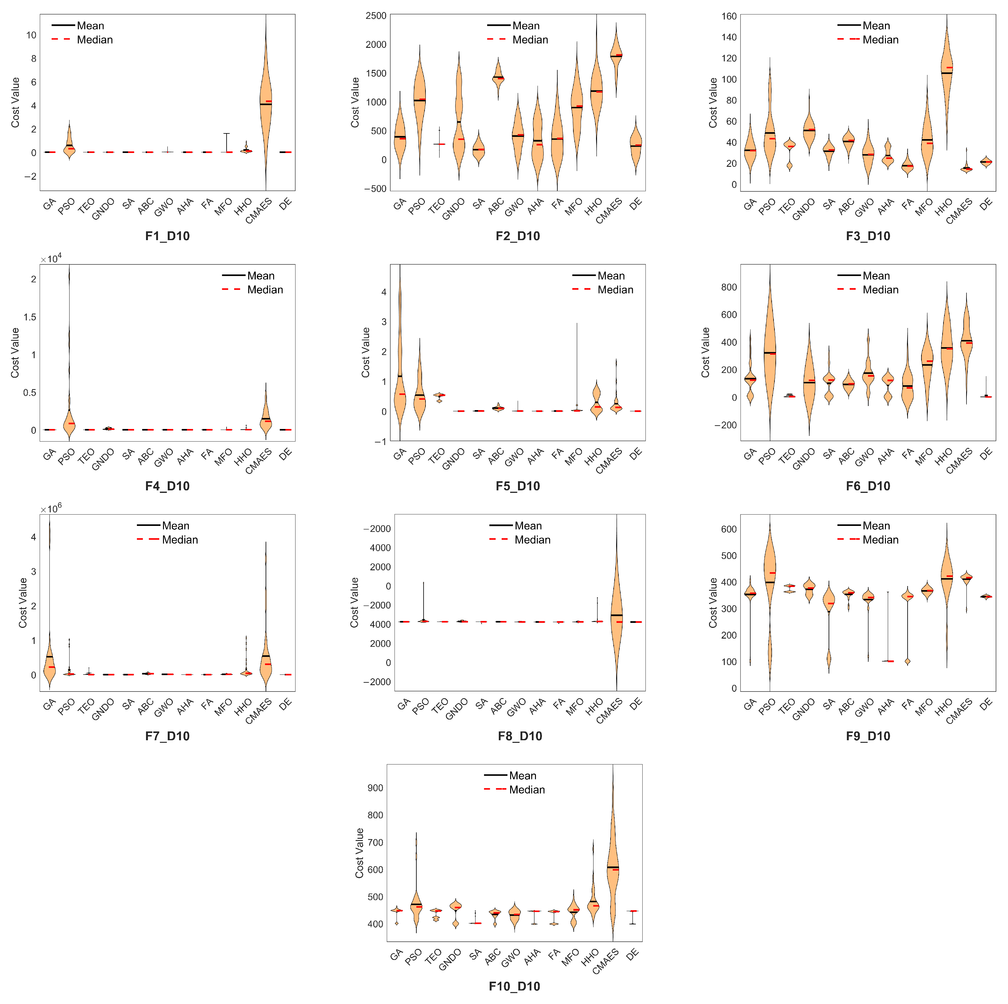
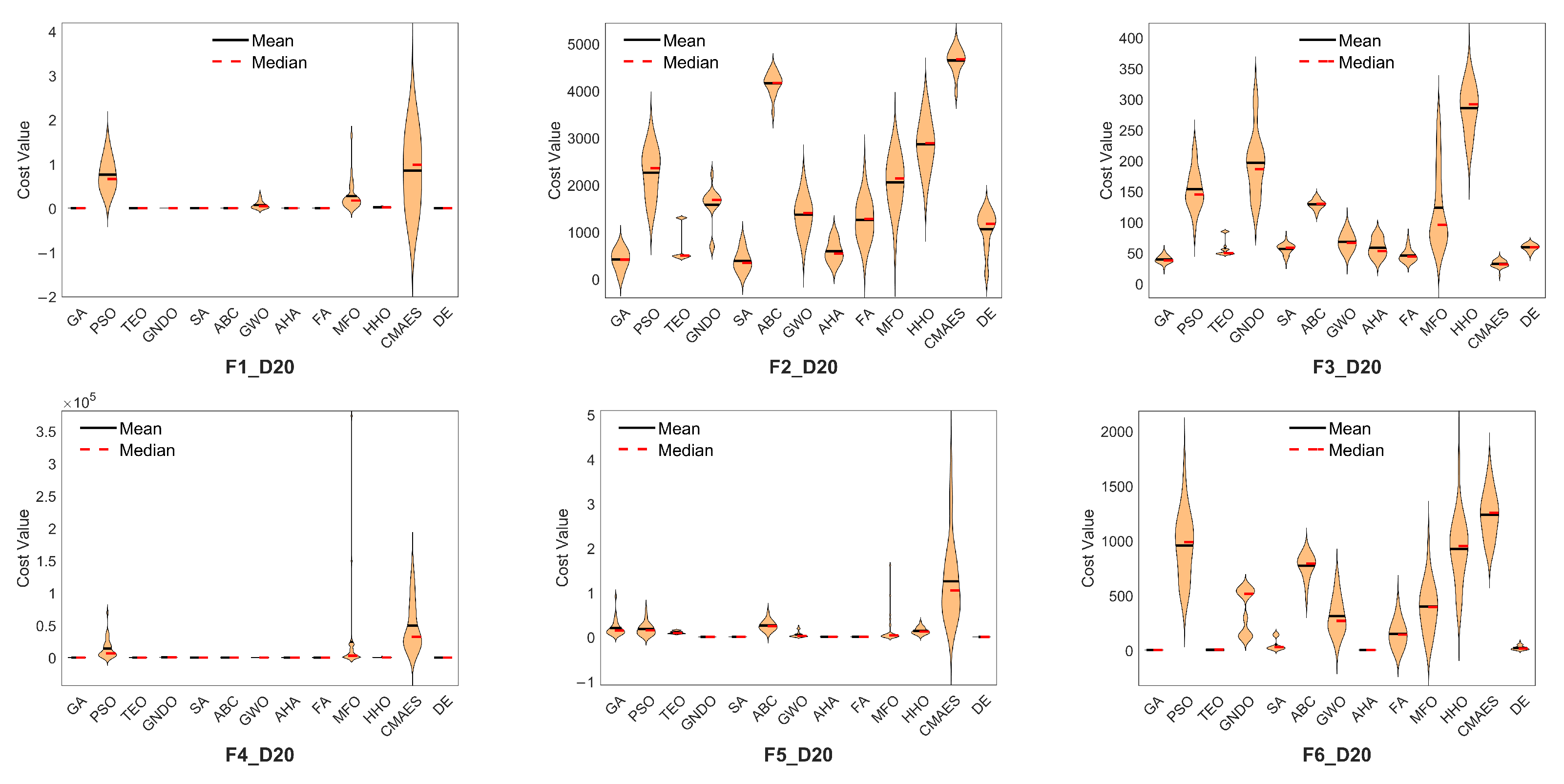
). Violin plots are used to visualize the performance distribution across 30 runs. Figure 2 illustrates the distribution of the best fitness values for a representative function (F6) in both 10D and 20D. The DE algorithm shows a more compact distribution, indicating consistent performance. LCA and BAS are excluded from the plot due to their significantly high error values. Complete violin plots for all functions are provided in Appendix B (Figure A1 and Figure A2).

Table 2. Statistical analysis of the median error metric for all the algorithms on CEC2020 (10D and 20D). DE is the reference algorithm in all comparisons.

Alg.	Wilcoxon	Friedman Test
Name	Test	SumRanks	MeanRanks	Rank
GA	+16/=0/−4	139	6.950	7
PSO	+20/=0/−0	226	11.300	13
TEO	+15/=0/−5	127	6.350	6
GNDO	+20/=0/−0	144	7.200	8
SA	+13/=0/−7	99	4.950	4
ABC	+18/=0/−2	161	8.050	9
GWO	+17/=0/−3	125	6.250	5
AHA	+14/=0/−6	77	3.850	3
BAS	+20/=0/−0	298	14.900	15
FA	+14/=0/−6	73	3.650	2
MFO	+20/=0/−0	162	8.100	10
LCA	+20/=0/−0	278	13.900	14
HHO	+20/=0/−0	216	10.800	11
CMAES	+17/=1/−2	219.5	10.975	12
DE	NA	55.5	2.775	1
		p-value = $5.20953\times {10}^{-33}$

presents the Friedman and Wilcoxon Signed-Rank test results for the comparative analysis of the meta-heuristic algorithms on the CEC2020 benchmark functions across 10D and 20D. The Friedman test reveals a highly significant difference among the algorithms with a p-value of $5.21\times {10}^{-33}$, indicating that the null hypothesis of equal performance is strongly rejected. The DE algorithm significantly ranked first, achieving the lowest average rank of 2.775, followed by FA (3.650), AHA (3.850), and SA (4.950). In contrast, BAS and LCA recorded the highest average ranks (14.9 and 13.9), reflecting their relatively poor optimization performance.

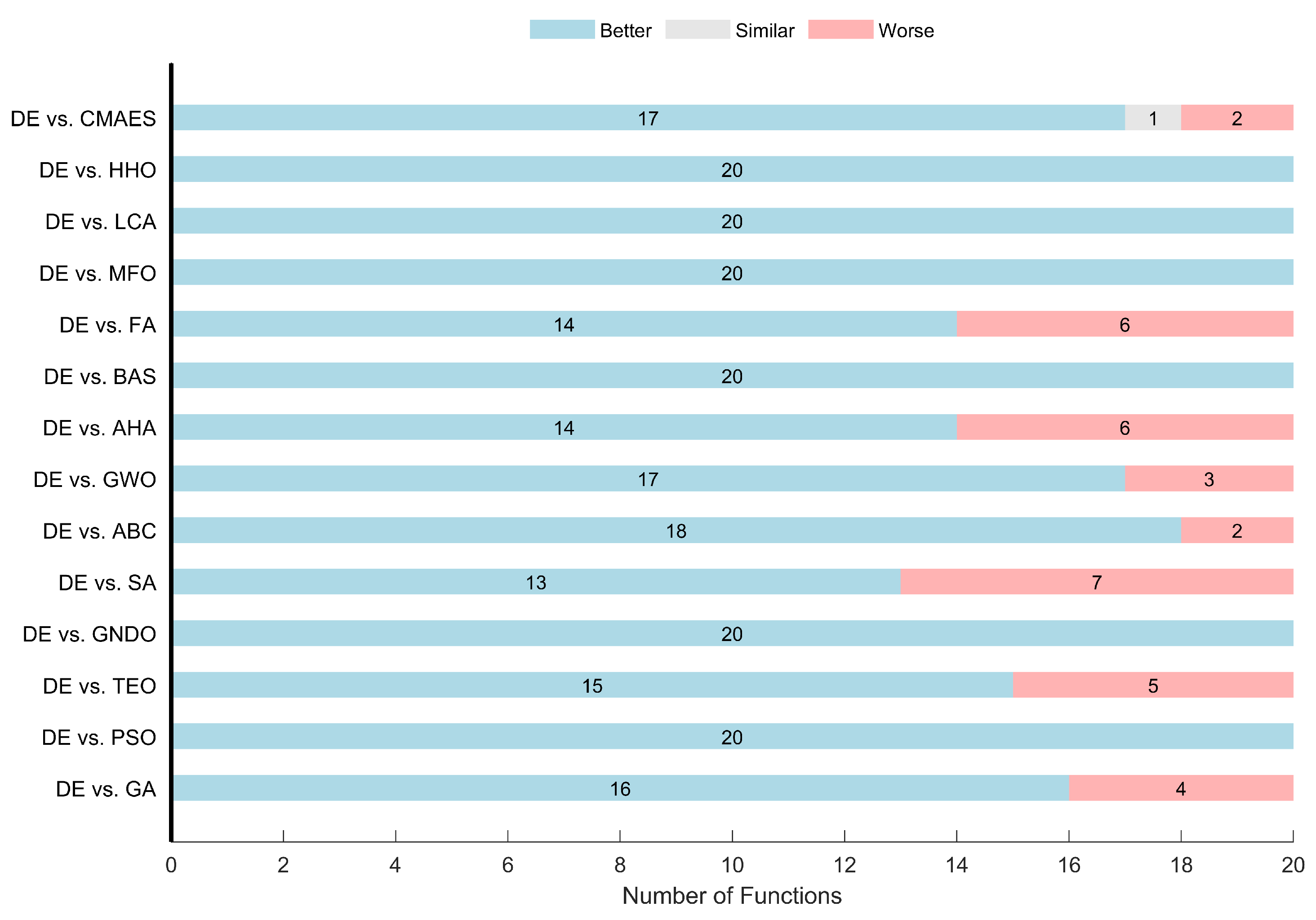
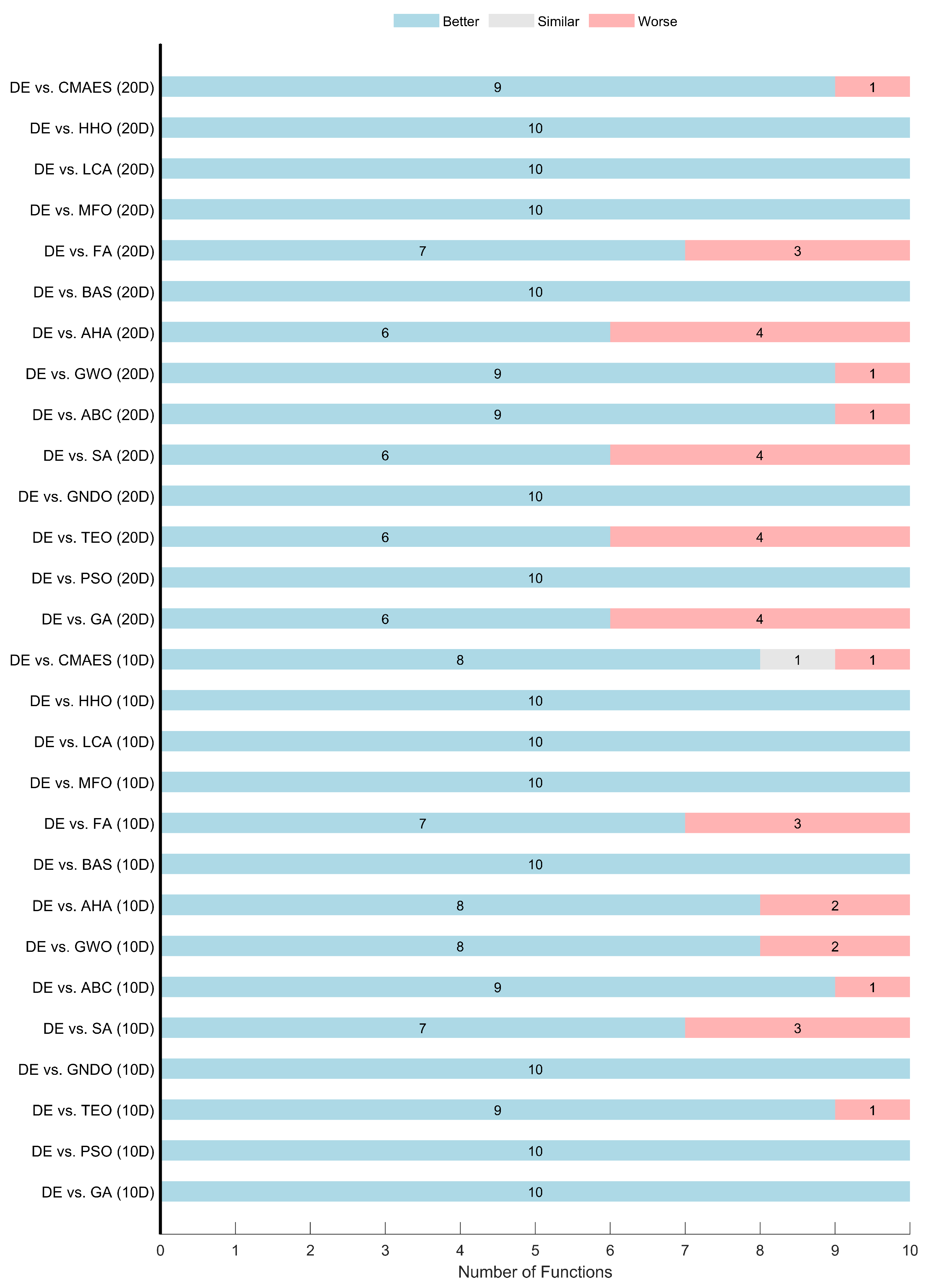
The Wilcoxon Signed-Rank test results in the same table provide a pairwise comparison against DE. DE outperformed every algorithm in at least 13 out of 20 functions, achieving perfect wins (+20, =0, −0) against multiple competitors such as PSO, GNDO, BAS, MFO, LCA, and HHO. Notably, SA, FA, and AHA represent the strongest challengers to DE, securing 7, 6, and 6 wins, respectively. Figure 3 visualizes the Wilcoxon test results from the algorithmic perspective. Figure 4 breaks down the analysis by dimension. Results in 10D and 20D are relatively consistent, highlighting the stability of DE across different problem sizes. However, a slight advantage is observed in 10D, where DE records more dominant wins.

Figure 5 presents a function-category-wise view. DE achieved complete dominance in Unimodal functions, winning all comparisons. In the Multimodal group, DE demonstrated competitive performance but showed relative weakness compared to some algorithms. It lost multiple comparisons against FA, TEO, and SA, each of which outperformed DE in 4 out of the 6 functions. GA and AHA showed comparable performance, each securing 3 wins against DE. Conversely, DE achieved a perfect win (6 out of 6) compared to PSO, GNDO, ABC, GWO, BAS, MFO, LCA, and HHO, reflecting its consistent superiority over these methods within this category.

For Hybrid functions, DE achieved consistent wins in 5 or 6 functions against most algorithms, losing only one comparison each to AHA, TEO, and GA. In the Composition functions, DE exhibited clear superiority, winning 6 out of 6 cases against GNDO, BAS, MFO, LCA, HHO, and CMAES. DE also achieved more wins than losses against ABC, AHA, and FA. It had a balanced performance (3 wins, 3 losses) against GWO and SA. These findings confirm that the DE algorithm not only performs well in unimodal functions but also maintains superior performance in complex hybrid landscapes, making it a suitable choice for integration into the ROS-based path-planning framework.

3.4. Time Complexity Analysis

Time complexity is a critical consideration for real-time robotic applications. This section analyzes the computational complexity of the DE algorithm and compares it against meta-heuristic optimization algorithms in both theoretical and practical contexts.

3.4.1. Asymptotic Time Complexity of the DE

The DE algorithm adopts the classical DE/rand/1/bin strategy with fixed control parameters ($F=0.5$, $CR=0.5$). It does not rely on memory-intensive components such as external archives, adaptation schemes, or historical tracking. This simple design minimizes computational overhead and simplifies the implementation, reducing execution delays. In each generation, the algorithm performs mutation and crossover operations followed by a fitness evaluation for each individual in the population.

For a population of size $N_p$, problem dimension D, and maximum number of generations G, the total time complexity can be approximated as $\mathcal{O}(G·N_p·D)$. This linear scaling in D and $N_p$ is one of the most efficient among evolutionary algorithms, especially when compared to adaptive or hybrid methods, which require additional memory or model computations. Therefore, the selected DE algorithm represents a time-optimal solution for ROS-based real-time path planning and control applications.

3.4.2. Practical Time Complexity Analysis

To assess the practical computational performance of the evaluated algorithms, we adopt four established time metrics: $T_0$, $T_1$, $T_2$, and $T_3$, as proposed in optimization benchmarking studies [62,68].

The metric $T_0$ measures the raw computational speed of the hardware by executing a standardized code snippet. All algorithms were executed on a machine with an Intel Core i7-6500U CPU (2.50–2.60 GHz), 8.00 GB RAM, Windows 11 Pro, and MATLAB R2024a. $T_1$ quantifies the inherent complexity of each benchmark function, independent of any algorithm, and is computed by averaging the time for 2000 function evaluations on CEC2020 test functions (10D and 20D).

In contrast, $T_2$ captures the time taken by each algorithm to perform the same number of function evaluations, thereby reflecting both algorithmic and problem-related complexity. The final metric, $T_3$, integrates all three previous metrics and is defined as shown in Equation (2). It represents the normalized algorithmic overhead beyond the inherent function cost, adjusted for hardware capability.

$$T_3={\displaystyle \frac{T_2-T_1}{T_0}}$$

(2)

Table 3. Time complexity results for all algorithms across all CEC2020 functions.

Dim.	Algorithm	T0	T1	T2	T3	Rank
10D	TEO	0.003873	0.027558	0.068143	10.478112	14
	GNDO	0.003873	0.027558	0.066113	9.954199	13
	AHA	0.003873	0.027558	0.060139	8.411786	11
	LCA	0.003873	0.027558	0.033791	1.609279	3
	GA	0.003873	0.027558	0.076754	12.701505	15
	SA	0.003873	0.027558	0.036201	2.231425	4
	PSO	0.003873	0.027558	0.046468	4.882279	10
	ABC	0.003873	0.027558	0.038284	2.769383	5
	GWO	0.003873	0.027558	0.045135	4.538192	9
	BAS	0.003873	0.027558	0.032749	1.340379	2
	FA	0.003873	0.027558	0.038518	2.829714	6
	MFO	0.003873	0.027558	0.043759	4.182754	8
	HHO	0.003873	0.027558	0.042279	3.800826	7
	CMAES	0.003873	0.027558	0.064992	9.664697	12
	DE	0.003873	0.027558	0.031462	1.008027	1
20D	TEO	0.003873	0.040130	0.052442	3.178742	11
	GNDO	0.003873	0.040130	0.049290	2.364859	8
	AHA	0.003873	0.040130	0.048204	2.084605	6
	LCA	0.003873	0.040130	0.031033	2.348605	7
	GA	0.003873	0.040130	0.074024	8.750716	15
	SA	0.003873	0.040130	0.030905	2.381669	9
	PSO	0.003873	0.040130	0.042173	0.527367	2
	ABC	0.003873	0.040130	0.035524	1.189035	3
	GWO	0.003873	0.040130	0.051319	2.888839	10
	BAS	0.003873	0.040130	0.025127	3.873428	12
	FA	0.003873	0.040130	0.034626	1.421036	4
	MFO	0.003873	0.040130	0.059170	4.915718	13
	HHO	0.003873	0.040130	0.032817	1.888033	5
	CMAES	0.003873	0.040130	0.073541	8.625960	14
	DE	0.003873	0.040130	0.039071	0.273529	1

presents the average time complexity metrics for all algorithms across the CEC2020 functions. Notably, the DE algorithm achieves the lowest $T_3$ value in both 10D and 20D scenarios, indicating the most efficient computation per unit hardware performance. Specifically, DE scores $T_3=1.008$ in 10D and $T_3=0.273$ in 20D, significantly lower than competing algorithms. These results confirm that DE not only leads in optimization accuracy but also in execution efficiency, making it an ideal candidate for real-time deployment in robotic systems.

4. The Proposed ROS Architecture for the Full ADS

This section details the implementation of the autonomous driving system (ADS), built entirely within the Robot Operating System (ROS) framework and deployed on a Raspberry Pi 4 in a 4WD prototype. The system integrates perception, localization, mapping, path planning, and control through a modular set of ROS nodes. The optimization core, Differential Evolution (DE), is fully embedded within both the path-planning and control nodes to enable real-time path generation and adaptive PID tuning. This deep integration motivates naming the algorithm “ROS-based Differential Evolution” (RDE), reflecting its customized deployment and execution within the ROS environment. The following subsections describe how DE is adapted and interfaced with the ROS components.

4.1. Overall View of the ROS System Architecture

Figure 6 illustrates the proposed ROS system’s architecture, comprising eight interconnected nodes in a closed-loop system. The Arduino node acts as the firmware, receiving PID controller parameters and desired velocities from the control node while publishing the motors’ current velocities, RPM values, and raw IMU readings. The Madgwick filter node processes raw IMU values to merge the accelerometer and gyroscope frames, providing a filtered IMU signal. The dead reckoning node calculates the car’s position using encoder data and publishes raw odometry.

The LiDAR node generates laser scan data, indicating distances to surrounding objects. These data are used by the Hector SLAM node to create a map and determine the car’s current location on it. The Extended Kalman Filter (EKF) node fuses the filtered IMU signal, Hector SLAM position, and raw odometry to produce refined odometry. The path-planning node uses the map and car pose as inputs, with the goal point aligned on the car’s heading at the maximum LiDAR range. If obstacles are detected, the proposed planner generates a collision-free path to maneuver around them.

Two control nodes are designed to perform two main tasks: the first is converting waypoint coordinates into velocities for the Arduino node, and the second is tuning PID gains for speed control. This implementation ensures continuous closed-loop operation, with DE integrated into the path-planning node and the control node. The following sections detail the functions and implementation of each node.

4.2. The Proposed Path-Planning Node

The path-planning node is the core component responsible for generating a collision-free path from the current pose to a dynamically selected goal. It relies on the real-time occupancy grid map published by the Hector-SLAM node. The node processes multiple steps as follows.

4.2.1. Search Space Boundaries

The search space boundaries are defined using the metadata provided by the Hector-SLAM node through the ‘map/metadata’ topic. This topic includes the origin $(x_{org},y_{org})$, map width $M_{width}$, height $M_{height}$ in cells, and the resolution $M_{res}$ in meters per cell. The boundaries $x_{min}, x_{max}, y_{min}, y_{max}$ are computed using Equation (3).

$$\begin{array}{cc}{x}_{min}& =x_{org},\hfill \\ \hfill y_{min}& =y_{org},\hfill \\ \hfill x_{max}& =x_{org}+(M_{width}\times M_{res}),\hfill \\ \hfill y_{max}& =y_{org}+(M_{height}\times M_{res})\hfill \end{array}$$

(3)

4.2.2. Start and Dynamic Goal Calculation

The start point $(x_s,y_s)$ is obtained from the car’s current pose ($x_{curr},y_{curr}$) in the ‘Filtered/odom’ topic published by the EKF node. At the same time, the heading of the start point ${\theta }_s$ is derived from the current orientation ${\theta }_{curr}$ in the same topic.

The goal point $(x_g,y_g)$ is the destination to which the planned path is directed. The core idea is to maintain the car’s motion along a straight line as long as no obstacles are present. When the road ahead is free, the goal is dynamically set along the car’s current heading at the farthest detectable point within the LiDAR’s sensing range ($L{D}_{max}=30$ m for Hokuyo UTM-30LX), as defined in Equation (4).

$$\begin{array}{cc}\hfill x_g& =x_s+L{D}_{max}·cos\left({\theta }_s\right),\hfill \\ \hfill y_g& =y_s+L{D}_{max}·sin\left({\theta }_s\right).\hfill \end{array}$$

(4)

However, if obstacles are detected ahead, such as parked vehicles, roadworks, or chicanes, the dynamic goal update is temporarily paused, and the planner generates intermediate waypoints to overtake the obstruction safely. Once the road is clear, the system resumes goal projection along the original heading to re-align with the initial path direction.

The computed goal point $(x_g,y_g)$ must lie within the valid bounds of the occupancy grid. If $x_g$ exceeds the grid limits, it is clamped based on the conditions in Equation (5). Then, the corresponding $y_g$ is updated to maintain alignment with the vehicle’s heading using Equation (6). Similarly, if $y_g$ violates the vertical boundaries, it is adjusted according to Equation (7), and $x_g$ is recalculated as per Equation (8).

$$x_g=\left\{\begin{array}{cc}{x}_{max},\hfill & \mathrm{if}{x}_s>x_{max},\hfill \\ x_{min},\hfill & \mathrm{if}{x}_s<x_{min},\hfill \\ x_g,\hfill & \mathrm{otherwise}.\hfill \end{array}\right.$$

(5)

$$y_g=y_s+(x_g-x_s)tan\left({\theta }_s\right)\mathrm{If}{x}_g\mathrm{is}\mathrm{adjusted}$$

(6)

$$y_g=\left\{\begin{array}{cc}{y}_{max},\hfill & \mathrm{if}{y}_s>y_{max},\hfill \\ y_{min},\hfill & \mathrm{if}{y}_s<y_{min},\hfill \\ y_g,\hfill & \mathrm{otherwise}.\hfill \end{array}\right.$$

(7)

$$x_g=x_s+{\displaystyle \frac{(y_g-y_s)}{tan\left({\theta }_s\right)}}\mathrm{If}{y}_g\mathrm{is}\mathrm{adjusted}.$$

(8)

4.2.3. Path Cost Calculation

The cost function used by the planner includes two components: the total Euclidean distance L and the cumulative obstacle penalty $p^T$. The total path length L is computed using Equation (9), where $(x_i,y_i)$ and $(x_{i+1},y_{i+1})$ are consecutive waypoints.

$$L=\sum _{i=1}^{n-1}\sqrt{{(x_{i+1}-x_i)}^2+{(y_{i+1}-y_i)}^2}$$

(9)

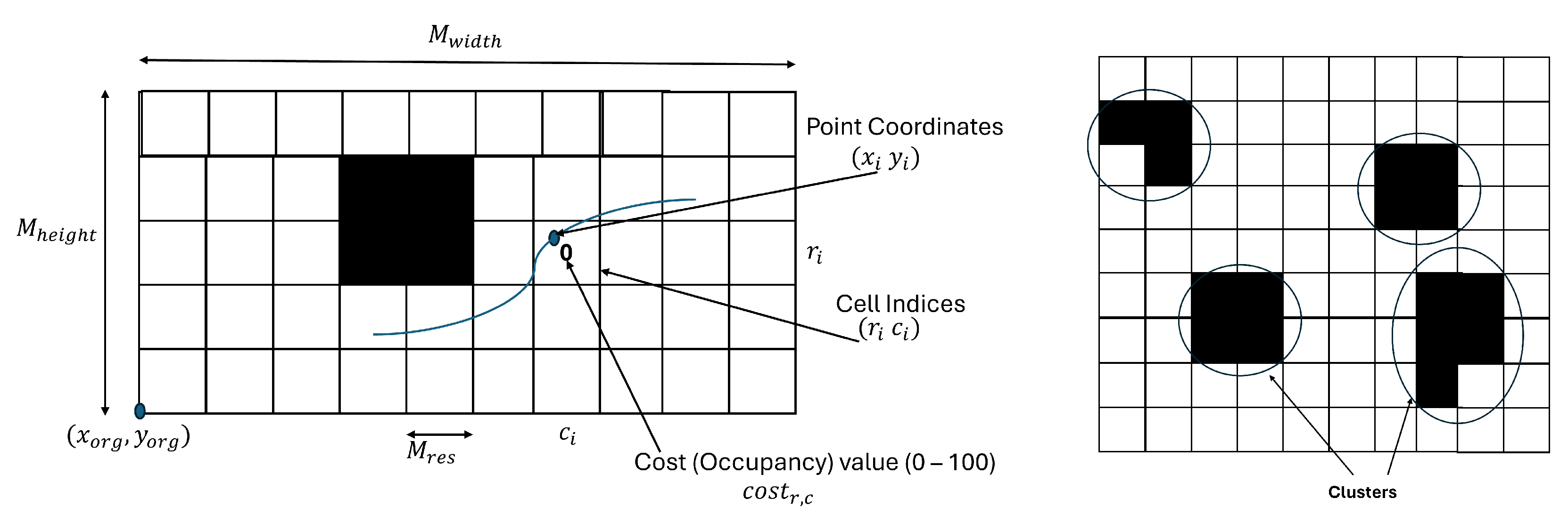
For each path point, the corresponding cell index $(r_i,c_i)$ in the occupancy grid is computed using Equation (10). The penalty $p_i$ is calculated from the cell’s occupancy value as shown in Equation (11). The total penalty $p^T$ is then computed by summing all point penalties according to Equation (12).

$$\begin{array}{cc}\hfill r_i& =round\left({\displaystyle \frac{x_i-x_{org}}{M_{res}}}\right)\hfill \\ \hfill c_i& =round\left({\displaystyle \frac{y_i-y_{org}}{M_{res}}}\right)\hfill \end{array}$$

(10)

$$p_i={\displaystyle \frac{Cos{t}_{r_i,c_i}}{100}}$$

(11)

$$p^T=\sum _{i=1}^n\left(p_i\right)$$

(12)

The final cost is calculated by combining the path length and penalty using Equation (13), where $\beta$ is set to 100 to strongly discourage paths that intersect with obstacles and n is the number of path points.

$$cost=L\ast (1+\beta p^T)$$

(13)

4.2.4. Obstacle Clustering

DBSCAN (Density-Based Spatial Clustering of Applications with Noise) is applied to the occupancy grid to estimate the number of obstacles in the environment. This algorithm identifies dense regions of high occupancy values and groups them into clusters, each representing a distinct obstacle [69]. The total number of obstacles $n_{obst}$ is defined as the number of such valid clusters. This value directly determines the number of waypoints used in the Differential Evolution optimization process. Figure 7 illustrates how the occupancy map and clustering are used during path evaluation.

4.2.5. Differential Evolution Optimization

The waypoint optimization is performed using the Differential Evolution (DE) algorithm, formulated to minimize the path cost defined in Equation (13). Each agent in the DE population represents a candidate path composed of $n_{obst}$ waypoints, where each waypoint $p_{j,i}^t=(x_{j,i}^t,y_{j,i}^t)$ belongs to the j-th path at iteration t. The population size $n_{pop}$ is set to 30.

The DE process starts with a random initialization of all paths. Each path $p_j^t$ is evaluated using the fitness function in Equation (13). Mutation is performed using the DE/rand/1 strategy in Equation (14), where three distinct paths $p_{r1}^t$, $p_{r2}^t$, and $p_{r3}^t$ are selected randomly, and the scaling factor F is set to 0.5 [70].

$$m_{j,i}^t=p_{r1,i}^t+F.(p_{r2,i}^t-p_{r3,i}^t)$$

(14)

The crossover step, defined in Equation (15), generates the child solution $u_{j,i}^t$ using the crossover probability $CR=0.5$. The child path $u_j^t$ is then evaluated. In the selection phase, the better path based on cost is retained, as shown in Equation (16). This process is repeated until the algorithm reaches a maximum number of iterations $T=10,000\times n_{obst}$ or converges when no improvement is observed below a tolerance of ${10}^{-8}$.

$$u_{j,i}^t=\left\{\begin{array}{cc}{m}_{j,i}^t\hfill & \mathrm{if} rand(0,1)\le CR\hfill \\ p_{j,i}^t\hfill & \mathrm{otherwise}\hfill \end{array}\right.$$

(15)

$$p_j^{t+1}=\left\{\begin{array}{cc}{u}_j^t\hfill & \mathrm{if} f\left(u_j^t\right)<f\left(p_j^t\right)\hfill \\ p_j^t\hfill & \mathrm{otherwise}\hfill \end{array}\right.$$

(16)

4.2.6. Failsafe Triggering Based on Path Validity

The path-planning node incorporates a built-in mechanism to assess the validity of the computed path in real time. The planner determines whether a collision-free path can be found within a fixed decision window. If no feasible path is found within ($t_{timeout}=250\mathrm{ms}$), the node publishes a Boolean flag ‘Path/valid’ = false.

The timeout value of 250 ms is chosen based on empirical profiling of the RDE planner’s runtime on the target hardware (Raspberry Pi 4B), where each complete optimization cycle averages 39.07 ms. This threshold enables multiple full planning attempts per cycle. This logic enhances the system’s safety, allowing fast failure detection while maintaining the system’s real-time performance.

4.2.7. Overall Path-Planning Node via ROS-Based Differential Evolution (RDE)

The path-planning node operates as a central component in the navigation framework, integrating all previous steps into a complete ROS-based optimization process. It subscribes to two topics from the Hector SLAM node: ‘Map/grid’ for the occupancy grid, ‘Map/metadata’ for map dimensions and resolution. Additionally, it subscribes to the ‘Filtered/odom’ topic from the EKF node to obtain the robot’s current pose. All steps are summarized in Algorithm 1, which outlines the whole execution logic of the node.

Algorithm 1: Path-Planning Node with RDE

Subscribe to ‘Map/grid’, ‘Map/metadata’, and ’Filtered/odom’ topics. Publish to ‘Path/waypoint’ and ‘Path/valid’ topics. Initialize DE parameters (F, $CR$) and set safety threshold ${\tau }_{cost}$, timeout $t_{timeout}$. while System is running do       Read ‘Map/metadata’ to obtain map dimensions.       Compute $x,y$ boundaries from map metadata.       Read ‘Filtered/odom’ to obtain current vehicle pose.       Set current pose as DE starting point.       Determine goal on heading line within LiDAR range.       Apply boundary constraints on goal coordinates.       Read ‘Map/grid’ to acquire occupancy data.       Construct cost function using Equations (9)–(13).       Apply DBSCAN clustering to identify $n_{obst}$.       Start timing: $t_{start}\leftarrow$ current time       Run DE to optimise path:       Initialize population ${\left\{p_j\right\}}_{j=1}^{nPop}$ with random paths.         for $t=1$ to T do               for each path j do                     Apply mutation: Equation (14)                     Apply crossover: Equation (15)                     Evaluate child path: Equation (13)                     Apply selection: Equation (16)               end for               Update best-so-far path.               if (current time $-t_{start})>t_{timeout}$ then                     Break and proceed to validation check.               end if         end for         Path Validity Check:         if best path is collision-free then               Publish ‘Path/valid’ = true         else               Publish ‘Path/valid’ = false         end if         Return best path.         Publish next waypoint on ‘Path/waypoint’.   end while

4.3. Control Node

The control node translates the path generated by the path planner into velocity commands for the robot actuators. It supports two vehicle configurations: a 4WD mechanism (used in this paper as the primary hardware) and an Ackermann-steered variant (presented as an extension). For both cases, it publishes the desired linear and angular velocities to the ‘Required/vel’ topic. Additionally, it employs a Differential Evolution (DE) algorithm to adaptively tune the PID gains based on current motion errors.

4.3.1. Modified Pure Pursuit

The control node utilizes a modified Pure Pursuit algorithm to convert waypoints into motion vectors. In the standard Pure Pursuit algorithm, the look-ahead distance $l_d$ is pre-determined as a parameter [71]. However, in this implementation, the look-ahead distance $l_d$ is dynamically computed as the Euclidean distance between the robot’s current position $(x_i,y_i)$ and the next waypoint $(x_n,y_n)$, as shown in Equation (17).

The desired orientation angle ${\theta }_n$ is calculated from the relative position of the waypoint using Equation (18). The drift angle $\Delta \theta$ is defined as the angular deviation between the current and desired orientations, as given in Equation (19).

$$l_d=\sqrt{{(x_n-x_i)}^2+{(y_n-y_i)}^2}$$

(17)

$${\theta }_n=arctan2\left({\displaystyle \frac{y_n-y_i}{x_n-x_i}}\right)$$

(18)

$$\Delta \theta ={\theta }_n-{\theta }_i$$

(19)

4.3.2. Velocity Command Generation

This subsection describes how the control node utilizes the outputs of the Pure Pursuit algorithm to compute the linear and angular velocity commands, taking into account the vehicle’s mechanical configuration.

4WD Differential-Drive Configuration

In the 4WD mechanism, the desired angular velocity ${\omega }_z^{req}$ is computed as a linear function of the drift angle $\Delta \theta$, following Equation (20). Here, the proportional gain $k_{\omega }$ determines the turning aggression and is set to a small value (typically 0.3) to rotate safely at a slow speed during turns.

The linear velocity $v_x^{req}$ is calculated using Equation (21) as a function of the look-ahead distance $l_d$ and the drift angle $\Delta \theta$. It is directly proportional to the normalized look-ahead distance $l_d/l_{max}$, which encourages the robot to speed up when the path is straight. Where $l_{max}$ is the maximum look-ahead range, e.g., 30 m for a UTM-30LX LiDAR.

Simultaneously, $v_x^{req}$ is inversely proportional to the absolute value of the drift angle, meaning the robot slows down in sharp turns to avoid instability. The gain $K_v$ scales the maximum velocity $v_{xmax}$, typically set to 0.3 for safe operation. The parameter $\beta$ (commonly 0.9) regulates how aggressively the linear speed is reduced in response to steering error.

$${\omega }_z^{req}=k_{\omega }·\Delta \theta$$

(20)

$$v_x^{req}=K_v·v_{xmax}·(1-\beta ·|\Delta \theta \left|\right)·{\displaystyle \frac{l_d}{l_{max}}}$$

(21)

Ackermann Steering Extension

For Ackermann-steered vehicles, the control node extends the Pure Pursuit algorithm by incorporating curvature-based path tracking. First, the required path curvature $\kappa$ is computed from the drift angle and look-ahead distance via Equation (22). The steering angle $\delta$ is derived from the curvature and wheelbase $W_b$ using Equation (23), where $W_b$ denotes the distance between front and rear axles. The steering angle is then directly assigned to the angular velocity command ${\omega }_z^{req}$ as shown in Equation (24).

The linear velocity $v_x^{req}$ is computed using Equation (25) in a similar manner to the 4WD configuration. It is directly proportional to the normalized look-ahead distance and inversely proportional to the curvature magnitude $\left|\kappa \right|$. This method ensures the vehicle slows down during tight curves (high curvature) and speeds up on straight paths (low curvature).

$$\kappa ={\displaystyle \frac{2sin(\Delta \theta )}{l_d}}$$

(22)

$$\delta =arctan(\kappa ·W_b)$$

(23)

$${\omega }_z^{req}=\delta$$

(24)

$$v_x^{req}=K_v·v_{xmax}·(1-\beta ·|\kappa \left|\right)·{\displaystyle \frac{l_d}{l_{max}}}$$

(25)

4.3.3. Adaptive PID Tuning via DE

In both configurations, the control node applies the DE algorithm to adaptively tune the PID gains for motor speed control. It receives the current velocities from the ‘Current/raw_vel’ topic and the current motor RPMs from the ‘Current/rpm’ topic. The DE algorithm minimizes the control error between desired and measured velocities by optimizing the PID parameters $(K_p,K_i,K_d)$ in real time. The tuned parameters are published on the ‘PID/params’ topic. This continuous adaptation improves stability and responsiveness under varying environmental and mechanical conditions.

4.3.4. Failsafe Stop Handling Based on Path Validity

The control node continuously monitors the Boolean flag ‘Path/valid’ published by the path-planning node. If false is received, it immediately commands a stop by publishing zero linear and angular velocities on ‘Required/vel’. It also publishes ‘Failsafe/stop’ = true, ensuring motor PWMs are disabled directly at the firmware level [72]. This behavior ensures a rapid and safe halt in case of failed planning attempts. Normal control resumes automatically once two consecutive planning cycles confirm valid replanning (‘Path/valid = true’). The complete logic of the control node is summarized in Algorithm 2.

Algorithm 2: Control Node

Initialize the DE algorithm parameters and PID gains. Initialize the required velocities as zeros. Subscribe to ‘Path/waypoint’, ‘Filtered/odom’, ‘Current/rpm’, ‘Current/raw_vel’, and ‘Path/valid’. Publish to ‘Required/vel’, ‘PID/params’, and ‘Failsafe/stop’. while System is running do       Read the subscribed topic: ‘Path/valid’.       if ‘Path/valid’ == false then            Immediately publish zero velocities on ‘Required/vel’.            Publish ‘Failsafe/stop’ = true.            Continue to next cycle.       else            Publish ‘Failsafe/stop’ = false.       end if       Read ‘Path/waypoint’ to obtain next desired point.       Read ‘Filtered/odom’ to obtain current pose.       Compute look-ahead distance from Equation (17).       Compute heading error using Equations (18) and (19).       if 4WD Mechanism then                                                                                                          ▹ 4WD Case            Compute required angular velocity: Equation (20).            Compute required linear velocity: Equation (21).       else if Ackerman Mechanism then                                                                                 ▹ Ackerman case            Calculate the desired steering angle using: Equations (22) and (23).            Calculate the required angular velocity: Equation (24).            Calculate the required linear velocity: Equation (25).       end if       Publish the required velocities on the topic ‘Required/vel’.       Read ‘Current/raw_vel’ and ‘Current/rpm’ to obtain current motor velocities.       Compute the velocity error.       if Error < tolerance then            Run the DE algorithm to update PID parameters.       end if       Publish PID parameters to ‘PID/params’. end while

4.4. Arduino Node: Kinematics and Control

The Arduino node interfaces directly with the vehicle’s hardware, managing the control and kinematics layers of the ADS. It subscribes to the topics ‘Required/vel’, ‘PID/params’, and ‘Failsafe/stop’, which provide the required velocities ($v_x^{req}$, $v_y^{req}$, ${\omega }_z^{req}$), PID gains, and the emergency stop flag, respectively. It publishes the current velocities (’current/raw_vel’), motors’ speed (’Current’/rpm), and IMU sensor readings (’Raw/imu’).

4.4.1. Inverse Kinematics: Obtain the Required Motor Values from Velocities

The Arduino node calculates motor RPM values from the required velocities using inverse kinematics based on the Mecanum omnidirectional model. Equations (26)–(29) define the required RPM values for each motor ($M_{FL,rpm}^{req}$, $M_{FR,rpm}^{req}$, $M_{RL,rpm}^{req}$, $M_{RR,rpm}^{req}$), considering the contributions of $v_x^{req}$, $v_y^{req}$, and ${\omega }_z^{req}$. Here, $M_{FL,rpm}^{curr}$, $M_{FR,rpm}^{curr}$, $M_{RL,rpm}^{curr}$, and $M_{RR,rpm}^{curr}$ represent the current RPMs of the front-left, front-right, rear-left, and rear-right motors, respectively.

$v_x^{req}$ is the required linear velocity in the x-direction, $v_y^{req}$ is the required linear velocity in the y-direction, and ${\omega }_z^{req}$ is the required angular velocity around the z-axis. $C_w$ is the wheel circumference, $L_w$ is the wheelbase (distance between the front and rear wheels), and $W_w$ is the track width (distance between the left and right wheels). For skid steering, $v_y^{req}$ is set to zero, simplifying the system such that the left and right sides of the vehicle move at uniform speeds [73].

$$M_{FL,rpm}^{req}=\left({\displaystyle \frac{v_x^{req}\times 60}{C_w}}\right)-\left({\displaystyle \frac{v_y^{req}\times 60}{C_w}}\right)-\left({\displaystyle \frac{{\omega }_z^{req}\times 60\times \left(L_w+W_w\right)}{4C_w}}\right)$$

(26)

$$M_{FR,rpm}^{req}=\left({\displaystyle \frac{v_x^{req}\times 60}{C_w}}\right)+\left({\displaystyle \frac{v_y^{req}\times 60}{C_w}}\right)+\left({\displaystyle \frac{{\omega }_z^{req}\times 60\times \left(L_w+W_w\right)}{4C_w}}\right)$$

(27)

$$M_{RL,rpm}^{req}=\left({\displaystyle \frac{v_x^{req}\times 60}{C_w}}\right)+\left({\displaystyle \frac{v_y^{req}\times 60}{C_w}}\right)-\left({\displaystyle \frac{{\omega }_z^{req}\times 60\times \left(L_w+W_w\right)}{4C_w}}\right)$$

(28)

$$M_{RR,rpm}^{req}=\left({\displaystyle \frac{v_x^{req}\times 60}{C_w}}\right)-\left({\displaystyle \frac{v_y^{req}\times 60}{C_w}}\right)+\left({\displaystyle \frac{{\omega }_z^{req}\times 60\times \left(L_w+W_w\right)}{4C_w}}\right)$$

(29)

For the Ackerman mechanism, only $v_x^{req}$ is considered, as $v_y^{req}$ and ${\omega }_z^{req}$ are set to zero. The single rear motor’s RPM ($M_{rear,rpm}^{req}$) is calculated using Equation (30). The steering angle $\theta$ is directly proportional to ${\omega }_z^{req}$, as defined in Equation (31) [74].

$$M_{rear,rpm}^{req}={\displaystyle \frac{v_x^{req}}{C_w}}\times 60$$

(30)

$${\theta }^{req}={\omega }_z^{req}$$

(31)

4.4.2. Obtain the Current Speed from Encoder

The Arduino node calculates the current RPM of each motor by interpreting the change in encoder ticks, denoted as $\Delta \mathrm{ticks}$, over a specific time interval $\Delta t$. The encoder disc is divided into counts_per_rev slots (typically, 20 in the 4WD), which determines its resolution. $\Delta \mathrm{ticks}$ is measured as the difference between the current and previous tick counts. The current motor speed $M_{i,rpm}^{curr}$ is computed using Equation (32), where $\Delta t$ is converted from milliseconds to minutes.

$$M_{i,rpm}^{curr}=\left({\displaystyle \frac{\Delta \mathrm{ticks}}{\mathrm{counts\_per\_rev}}}\right)\times \left({\displaystyle \frac{60,000}{\Delta t}}\right)$$

(32)

4.4.3. Apply the PID Control

The Arduino node applies a PID controller to ensure the motors operate at the desired speed. The error e is defined as the difference between the required RPM $M_{i,rpm}^{req}$ and the current RPM $M_{i,rpm}^{curr}$, as indicated in Equation (33). The PID controller then generates a control signal using this error, combining proportional $K_p$, integral $K_i$, and derivative $K_d$ components as shown in Equation (34).

$$e=M_{i,rpm}^{req}-M_{i,rpm}^{curr}$$

(33)

$$PID=K_p·e+K_i·{\int }_0^{t}e\left(\tau \right)d\tau +K_d·{\displaystyle \frac{de}{dt}}$$

(34)

The control signal from the PID controller determines both the magnitude and direction of each motor’s actuation. The PWM value $M_{i,pwm}^{new}$ adjusts the motor speed and is computed as the absolute value of the PID output using Equation (35). The direction $M_{i,dir}^{new}$ is determined by the sign of the PID signal, as given in Equation (36). A positive value drives the motor forward, a negative value drives it in reverse, and zero stops the motor. The same logic is applied to control the steering angle, which is continuously adjusted until it matches the desired value ${\theta }^{req}$.

$$M_{i,pwm}^{new}=\left|PID\right|$$

(35)

$$M_{i,dir}^{new}=\left\{\begin{array}{cc}\mathrm{Forward}\hfill & \mathrm{if}PID>0\hfill \\ \mathrm{Reverse}\hfill & \mathrm{if}PID<0\hfill \\ \mathrm{Stop}\hfill & \mathrm{if}PID=0\hfill \end{array}\right.$$

(36)

4.4.4. Forward Kinematics: Obtain the Velocity from the Motor Values

The Arduino node applies forward kinematics to compute the current linear and angular velocities from the motor RPM values. For the Mecanum model, the forward kinematic Equations (37)–(39) calculate the current velocities ($v_x$, $v_y$, and ${\omega }_z$) based on the current RPM values of the four motors: $M_{FL,rpm}^{curr}$, $M_{FR,rpm}^{curr}$, $M_{RL,rpm}^{curr}$, and $M_{RR,rpm}^{curr}$

$$v_x=\left({\displaystyle \frac{M_{FL,rpm}^{curr}+M_{FR,rpm}^{curr}+M_{RL,rpm}^{curr}+M_{RR,rpm}^{curr}}{4\times 60}}\right)\times C_w$$

(37)

$$v_y=\left({\displaystyle \frac{-M_{FL,rpm}^{curr}+M_{FR,rpm}^{curr}+M_{RL,rpm}^{curr}-M_{RR,rpm}^{curr}}{4\times 60}}\right)\times C_w$$

(38)

$${\omega }_z=\left({\displaystyle \frac{-M_{FL,rpm}^{curr}+M_{FR,rpm}^{curr}-M_{RL,rpm}^{curr}+M_{RR,rpm}^{curr}}{4\times 60}}\right)\times {\displaystyle \frac{C_w}{(L_w/2+W_w/2)}}$$

(39)

In the differential drive and skid-steering models, the y-component $v_y$ is neglected. In the Ackerman model, the x-component $v_x$ is derived from $M_{rear,rpm}^{curr}$ using Equation (40). The angular velocity ${\omega }_z$ is then set to the current steering angle ${\theta }^{curr}$ as shown in Equation (41).

$$v_x={\displaystyle \frac{M_{rear,rpm}^{curr}\times C_w}{60}}$$

(40)

$${\omega }_z={\theta }^{curr}$$

(41)

4.4.5. Failsafe Motor Stop via Direct Override

The Arduino node supports a direct override mechanism that bypasses the PID and kinematics control layers, enhancing safety in emergency scenarios where planning fails. A Boolean topic ‘Failsafe/stop’ is subscribed to by the Arduino. When this flag is set to ‘true’, the node immediately disables all motor PWMs and sets their directions to ‘Stop’, regardless of the current PID output or requested velocities [72]. This logic ensures a low-latency halt in hardware, avoiding the delay introduced by PID control convergence. The normal control resumes when the flag is reset to ‘false’.

4.4.6. Overall Arduino Node

The current velocities computed through forward kinematics are published on the ‘Current/raw_vel’ topic, while the RPM values of all motors are shared via the ‘Current/raw_rpm’ topic. The node also transmits IMU sensor data through the ‘Raw/imu’ topic. The overall steps of the Arduino node are illustrated in Algorithm 3. This node represents the ADS firmware, which is responsible for handling the hardware layer, control actions, and kinematics layer.

Algorithm 3: Arduino Node Firmware

Setup and configure all the input and output pins. Subscribe to the ‘Required/vel’, ‘PID/params’, and ‘Failsafe/stop’ topics. Publish the ‘Current/raw_vel’, ‘Current/rpm’, and ‘Raw/imu’ topics. while System is running do       Check Failsafe Flag       Read the subscribed topic: ‘Failsafe/stop’ to check the path validity.       if ‘Failsafe/stop’ == true then            Immediately stop all motors (PWM = 0, Direction = Stop).            Continue to next loop cycle.       end if       Read the subscribed topic: ‘Required/vel’ to obtain the desired velocities.       Read the subscribed topic: ‘PID/params’ to obtain the PID gains.       Apply the IK to obtain the desired motor RPMs:       if 4WD Mechanism then            Apply the IK to obtain required motor RPMs from desired velocities: Equations (26)–(29).       else if Ackerman Mechanism then            Obtain the required rear motor RPM using: Equation (30).            Obtain the desired steering angle: Equation (31).       end if       Get the current motor RPMs from the encoder readings: Equation (32).       Calculate the error between the desired PWM and current PWM using Equation (33).       Apply the PID controller using Equation (34).       Set the new motor PWMs and directions based on the PID values: Equations (35) and (36).       Apply the FK to obtain the current motor RPMs:       if 4WD Mechanism then            Apply FK to obtain the new current velocities: Equations (37)–(39).       else if Ackerman Mechanism then            Obtain the current velocities using Equations (40) and (41).       end if       Publish the new current velocity on the topic ‘Current/raw_vel’.       Publish the new motor RPMs on the topic ‘Current/rpm’.       Read and Publish the current IMU sensor data on topic ‘Raw/imu’. end while

4.5. Supporting ROS Nodes

The proposed system relies on additional standard ROS nodes for LiDAR input, mapping, localization, and sensor fusion. These nodes are based on widely used ROS packages and libraries. While they are not part of the contributions of this work, they form the foundational infrastructure upon which the proposed methodology operates.

4.5.1. Dead Reckoning Node: Raw Odometry

The dead reckoning node calculates the car’s position $(x,y)$ and orientation $\theta$ based on its previous state and current velocities $v_x$, $v_y$, and ${\omega }_z$ provided by the Arduino node [75]. Starting with the current position $(x^t,y^t)$ and orientation ${\theta }^t$, the updated position $(x^{t+1},y^{t+1})$ and heading ${\theta }^{t+1}$ are calculated after a time interval $\Delta t$. The updates are performed using Equations (42)–(44), which account for linear and angular motion.

$$x^{t+1}=x^t+(v_x·cos\left({\theta }^t\right)-v_y·sin\left({\theta }^t\right))\times \Delta t$$

(42)

$$y^{t+1}=y^t+(v_x·sin\left({\theta }^t\right)+v_y·cos\left({\theta }^t\right))\times \Delta t$$

(43)

$${\theta }^{t+1}={\theta }^t+{\omega }_z\times \Delta t$$

(44)

The node subscribes to the ‘current/raw_vel’ topic to access the latest velocities and calculates the updated position and orientation. It publishes these values as odometry on the ‘Raw/odom’ topic. While useful, dead reckoning is prone to errors from slippage and encoder noise. To improve accuracy, these data are fused with other pose readings, providing a refined estimate of the car’s location.

4.5.2. LiDAR Node

The LiDAR sensor used in the study is the Hokuyo UTM-30LX, a compact 2D LiDAR sensor. It has a wide scanning angle of 270 and a long detection range of 30 m. The speed of the scan is 25 ms, which means it can provide 40 frames of scan per second. The angular resolution is $0.25$, dividing the 270 field-of-view into 1080 angles. It operates on a 12 V DC power source with a maximum current of 1A [76]. It was first tested using the UrgBenriPlus software (version 2.2.0, rev.274) by Hokuyo [77] to ensure that the LiDAR is functioning correctly.

The ROS has a built-in library called ‘urg_node,’ compatible with the Hokuyo UTM-30LX LiDAR (Hokuyo Automatic Co., Ltd., Osaka, Japan) [78]. This node reads LiDAR data via USB and publishes them to the ‘laser’ topic, formatted as a ‘sensor_msgs/LaserScan’ message. This message includes the scan range, resolution, minimum and maximum ranges, and arrays for distances and intensities [79].

4.5.3. Madgwick Filter Node

The Madgwick filter is applied to the IMU data to merge the accelerometer and gyroscope data into one frame. The filter estimates the real-time orientation by combining the accelerometer data with the gyroscope data relative to the Earth’s frame. This fusion process corrects any drift in the gyroscope sensor [80].

This filter is fully implemented in a built-in ROS package named imu-filter-madgwick [81]. The Madgwick filter node subscribes to the raw readings of the IMU sensor, published in the ‘Raw/imu’ topic by the Arduino node. It publishes a new topic, ‘Filtered/imu’, containing the corrected orientation and the fused IMU data.

4.5.4. Mapping Node: Hector SLAM

The SLAM (Simultaneous Localization and Mapping) algorithm is a method that is used for real-time mapping and navigation. Hector SLAM is a specific implementation of the SLAM algorithm mainly designed to work with the LiDAR sensor. It generates a dynamic environment map, identifies obstacles, and estimates the vehicle’s location within the map [82].

The Hector Slam node is implemented using the built-in ROS hector slam library [83]. The implemented node subscribes to the ‘laser’ topic from the LiDAR node, which includes the LiDAR scan data. It publishes three topics: ‘Map/metadata’ for map dimensions and resolution, ‘Map/grid’ for the occupancy values, and ‘Map/pose’ for the vehicle’s current position.

4.5.5. Extended Kalman Filter (EKF) Node

The Extended Kalman Filter (EKF) node fuses data from the dead reckoning odometry, filtered IMU readings, and SLAM-derived position to estimate a more accurate and reliable vehicle location [84]. This node is implemented using the standard ROS implementation described in [85]. It subscribes to ‘Filtered/imu’, ‘Raw/odom’, and ‘Map/pose’ topics for IMU data, encoder-based odometry, and SLAM position, respectively. The corrected pose, orientation, and velocity are published on the ‘Filtered/odom’ topic.

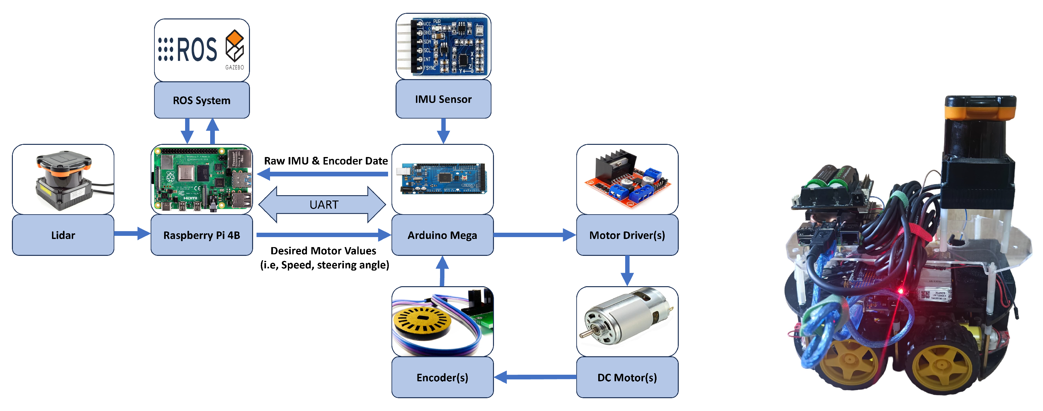
5. Hardware Implementation of the 4WD Robot

Figure 8 illustrates the hardware architecture of the modified 4WD robotic car. It is a modified version of the original Elegoo V4 smart car [86]. It comprises four 6–10 V geared DC motors with a 7.4 V lithium battery. The car is supported by an MPU-6050 IMU sensor (TDK InvenSense Inc., Sunnyvale, CA, USA) to measure its orientation. The original setup uses two TB6612 motor drivers (Toshiba Corporation, Tokyo, Japan), each controlling a pair of motors on the left and right sides, forming a two-wheel differential drive.

This setup is upgraded to four L298N drivers, enabling independent control of all four motors in a four-wheel differential drive configuration [87]. Rotary encoders (KY-040) are added to each motor to measure the speed and RPM [88].

The HOKUYO UTM-30LX LiDAR (Hokuyo Automatic Co., Ltd., Osaka, Japan) is mounted on a third layer of the car to map the surrounding environment. A dedicated 11.1 V LiPo lithium battery supplies the LiDAR with a 2000 mAh capacity. The battery voltage can decrease over time from 11.2 V to less than 10.8 V, which is insufficient to operate the LiDAR. Therefore, a step-up boost converter (XL6009 by Xlsemi Microelectronics Co., Ltd., Shanghai, China) is used to maintain the voltage at approximately 12 V [89].

Due to the additional hardware added to the Elegoo V4 car, the Arduino Uno is replaced with an Arduino Mega. The Arduino Mega is responsible for the car’s low-level control, including the motor speed control, reading encoder data, and IMU sensor data. The primary controller is the Raspberry Pi 4B, on which the whole ROS software, Noetic version is installed to implement the stages of the ADS. It is connected to Arduino and LiDAR via the UART protocol. The Raspberry Pi is supplied with a separate UPS circuit of type X728 V2.3 and two 18,650 batteries to ensure a safe power connection [90].

6. Pid Transient Response

This section compares the transient response performance between the proposed adaptive DE-tuned PID controller and a conventional Ziegler–Nichols (ZN) tuned PID controller. The objective is to assess the dynamic behavior of both approaches under nominal conditions and disturbance.

6.1. Traditional PID Control

In the traditional closed-loop control setup, the control cycle begins by setting the desired motor speed. The encoder measures the actual motor speed, which is compared to the desired speed to generate the error signal. The PID controller uses the error signal to generate the control signal, which combines proportional, integral, and derivative components. This signal is then sent to the motor driver to update the motor speed accordingly. The loop continues until the error is minimized.

The tuning of the PID controller has a critical impact on the system’s transient performance. A widely used tuning approach is the Ziegler–Nichols (ZN) method, where the integral and derivative gains are initially set to zero, and the proportional gain is gradually increased until the system output exhibits sustained oscillations [91]. The corresponding gain is called the ultimate gain $K_u=2.9$, and the oscillation period is $P_u=1.4$ s. These values were obtained experimentally, and then the ZN tuning rules yield the PID parameters: $K_p=1.75$, $K_i=2.5$, and $K_d=0.3063$ [92].

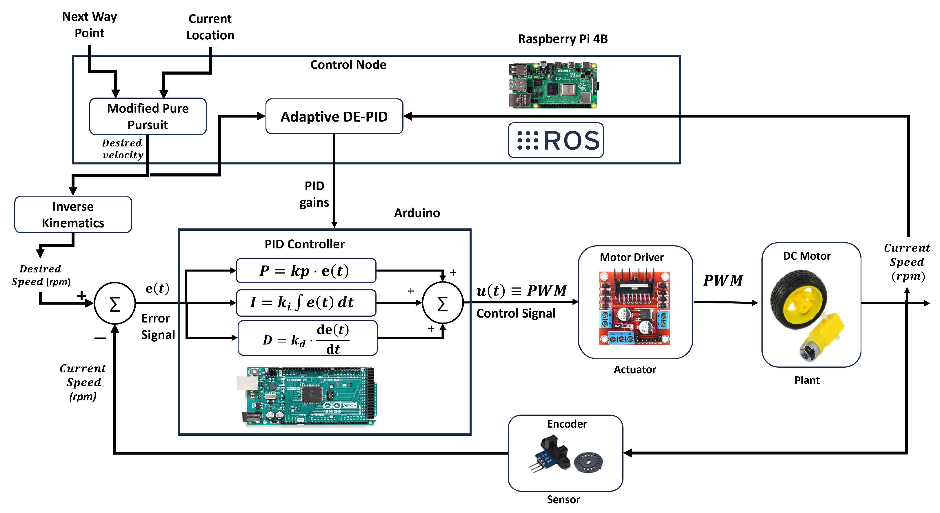
6.2. Adaptive DE-Tuned PID Control

Figure 9 illustrates the architecture of the adaptive PID control system, composed of the control node (Section 4.3) and the Arduino node (Section 4.4). In the complete system, the control node receives waypoint and localization data, generating the desired speed using the modified Pure Pursuit algorithm, which is sent to the Arduino.

The Arduino compares the desired speed (converted to RPM using inverse kinematics) with the actual motor speed from the encoders and computes the control signal using the PID logic. Meanwhile, the control node runs a Differential Evolution (DE) optimization algorithm every 3 s to adaptively update the PID gains in real time based on the current control error. This dual-feedback structure improves convergence, accelerates error reduction, and enhances robustness.

6.3. Experiment Setup

In this test, the modified Pure Pursuit algorithm is temporarily disabled to isolate the PID control loop performance. The system is set at a constant velocity reference, and the motor is commanded to run at maximum duty cycle (normalized to 1), allowing evaluation of the transient and disturbance response.

The experiment involves driving the motor at full duty cycle and monitoring the system’s response in two phases: (1) the start-up phase, where the system accelerates from a standstill state to the target speed, and (2) the recovery phase, where a temporary external load disturbance is applied for 1 s, followed by system recovery.

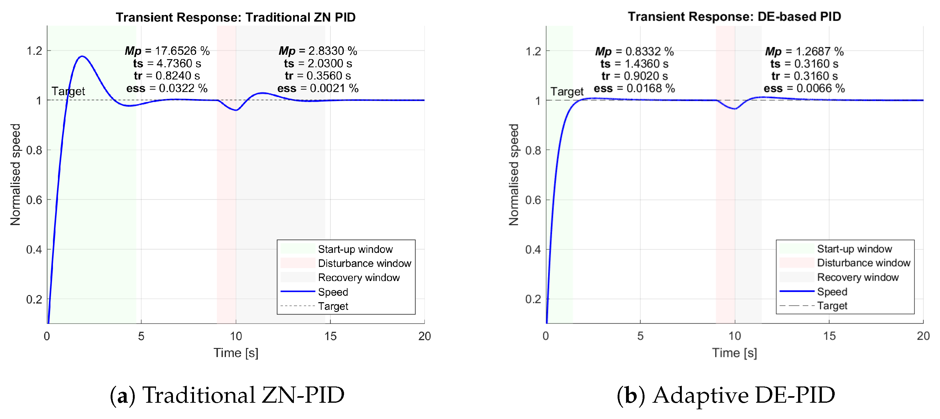
During both phases, key transient metrics are measured, including rise time ($t_r$), settling time ($t_s$), maximum overshoot ($M_p$), and steady-state error ($e_{ss}$). These indicators provide insight into how quickly and accurately each controller stabilizes the motor speed.

6.4. Transient Response Analysis

Figure 10 shows the transient responses of both controllers, while

Table 4. Transient-response metrics of the proposed adaptive DE-PID controller versus a conventional Ziegler–Nichols (ZN) PID controller.

Controller	Phase	${\mathit{t}}_{\mathit{r}}$ [s]	${\mathit{t}}_{\mathit{s}}$ [s]	${\mathit{M}}_{\mathit{p}}$ [%]	${\mathit{e}}_{\mathbf{ss}}$ [%]
Adaptive DE-PID (proposed)	Start-up	0.9020	1.4360	0.8332	0.0168
	Recovery	0.3160	0.3160	1.2687	0.0066
ZN-PID (baseline)	Start-up	0.8240	4.7360	17.6526	0.0322
	Recovery	0.3560	2.0300	2.8330	0.0021

summarizes the key performance indicators.

In the start-up phase, the proposed DE-PID achieved significantly reduced overshoot ($M_p=0.83\%$) compared to the ZN-PID ($M_p=17.65\%$), marking a 95% improvement. Additionally, the settling time improved by over 69% (from 4.74 s to 1.44 s), while maintaining a comparable rise time ($t_r$ increased slightly from 0.8240 s to 0.9020 s). Despite the marginally slower rise, the DE-PID effectively suppressed oscillations and converged faster with minimal steady-state error ($e_{ss}=0.0168\%$).

In the recovery phase, following the disturbance, the DE-PID controller again outperformed the ZN-PID. It achieved an 84% reduction in settling time (from 2.03 s to 0.316 s) and a 55% reduction in overshoot (from 2.83% to 1.27%). While the ZN-PID produced a slightly lower $e_{ss}$ (0.0021% vs. 0.0066%), this minor trade-off is outweighed by the substantial gains in transient response and stability. These results validate the robustness and adaptability of the proposed DE-tuned PID controller, particularly under dynamic conditions and load variations.

7. Ads Validation on Driving Scenarios Using 4WD

This section presents the experimental validation of the proposed ADS on the 4WD robotic platform. It includes the evaluation of key functional tasks such as the failsafe mechanism and performance in realistic driving scenarios.

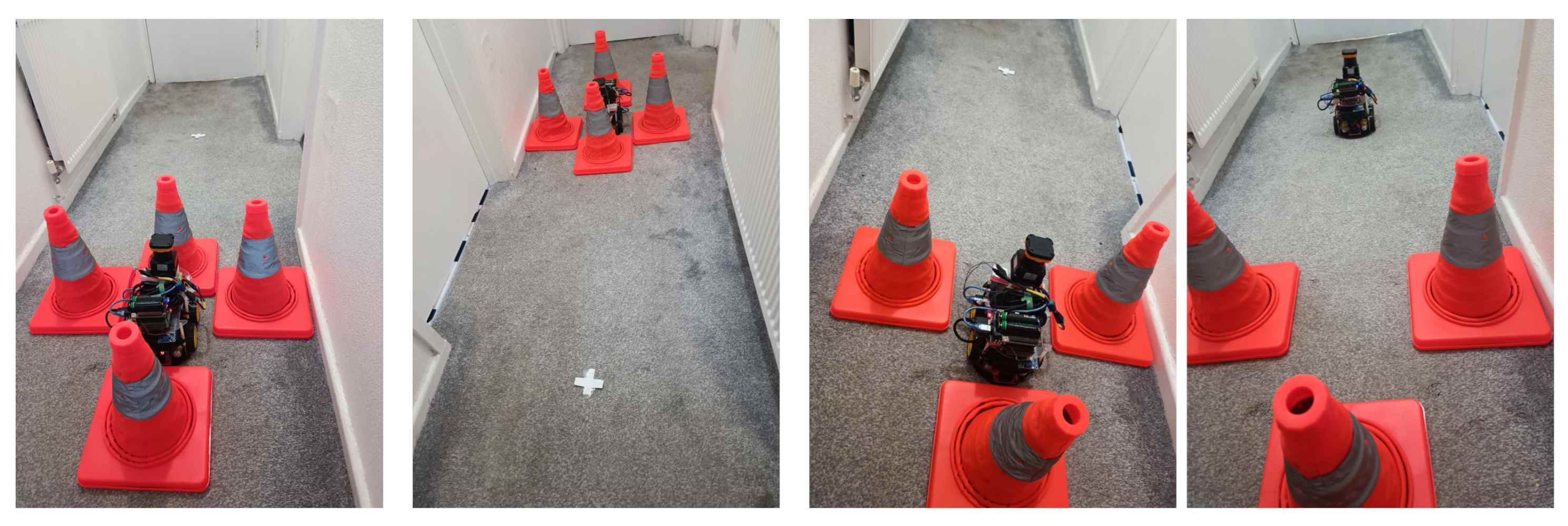
7.1. Failsafe Validation

A blocked-corridor stress test is performed to evaluate the failsafe mechanism. Four traffic cones are tightly positioned around the stationary 4WD robot, forcing all candidate paths to intersect with obstacles. As expected, the RDE planner returned no feasible solution, triggering the ‘Path/valid’ flag to switch to false within the 250 ms cycle window. In response, the control node immediately issued zero linear and angular velocity commands and activated the ‘Failsafe/stop’ flag. This effectively disabled motor output at the firmware level, keeping the vehicle fully immobilized.

After 2 s, the front cone was manually removed, creating a clear path forward. Within the subsequent two planning cycles (0.5 s), the ‘Path/valid’ flag reverted to true, allowing the control node to resume velocity commands and reset the ‘Failsafe/stop’ flag. The robot successfully departed from its initial position and advanced towards the target goal. Figure 11 illustrates both the blocked and cleared corridor scenarios during the test.

7.2. Driving Scenarios

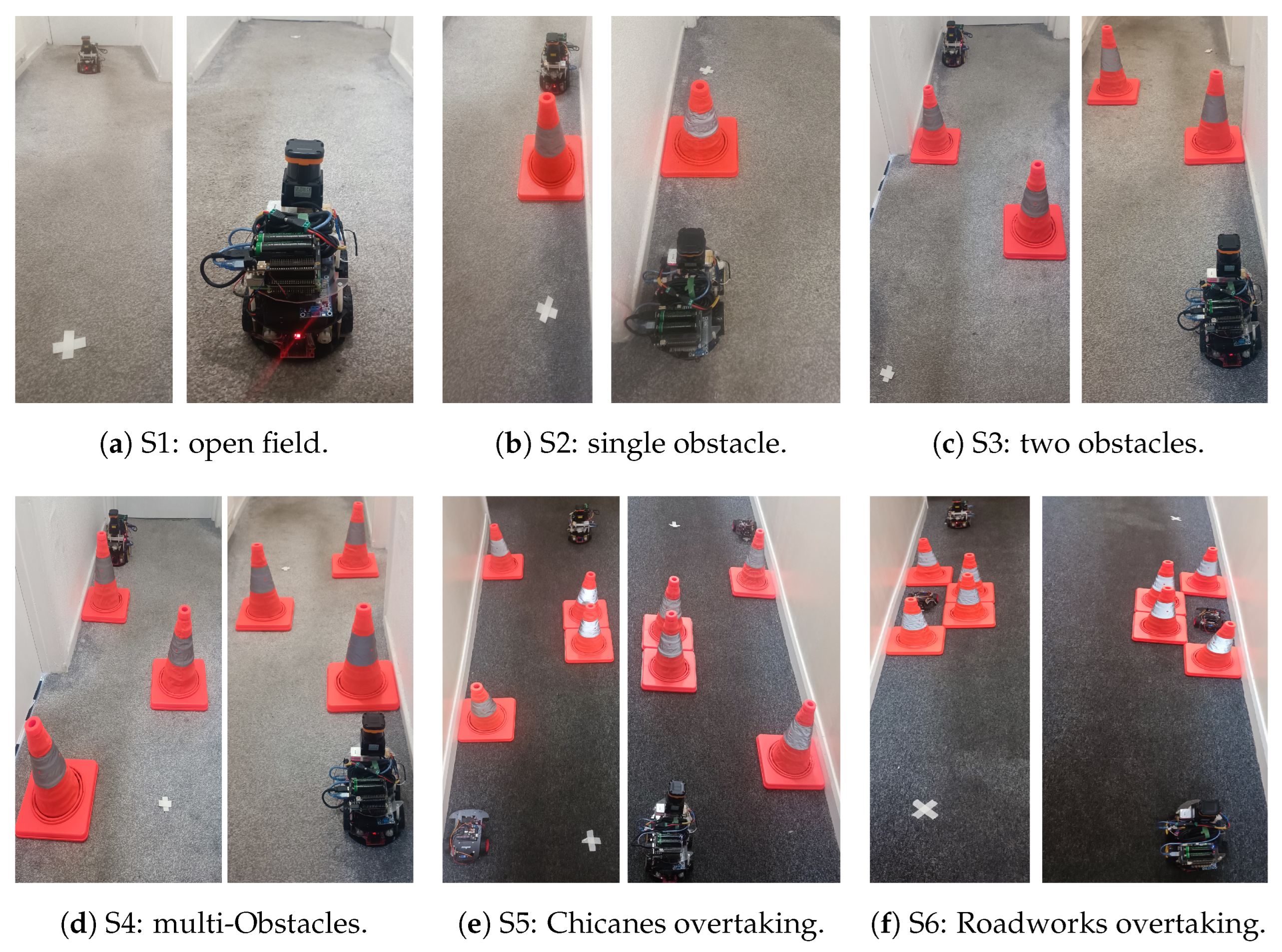
The 4WD model is validated against six simulated driving scenarios, two of which are based on the perception hazards outlined in the UK Highway Code theory book. The objective of the experiment is to ensure that the car can follow the path generated by the RDE algorithm without hitting any obstacles, thereby proving the correct integration of all nodes in the ADS pipeline.

The first scenario is an open-field scenario with no obstacles, in which the car must move from the starting point to the endpoint, as shown in Figure 12a. The second scenario is a single chicane obstacle between the start and endpoints, as seen in Figure 12b. The third and fourth scenarios consist of two and three chicanes, as in Figure 12c and Figure 12d, respectively. The fifth and sixth scenarios are constructed using four chicanes to simulate two challenging real-life driving scenarios: the chicanes overtaking and the overtaking of roadworks and parked cars, as seen in Figure 12e and Figure 12f, respectively.

Chicanes are traffic-calming methods that convert straight paths into curves, forcing the drivers to slow down and enhancing pedestrian safety in residential areas [93]. However, it can increase the risk of collision if not navigated properly, especially for inexperienced drivers. Moreover, urban chicanes are designed to accommodate only one vehicle at a time, which makes it more hazardous. Aydin et al. evaluated the chicanes scenarios using a driving simulator and reported a 43% accident rate in such scenarios, nearly half of all tests [94]. A similar real-world setup is prepared for this study, as illustrated in Figure 12e.

Roadwork overtaking is one of the most common everyday driving situations, especially in the UK. Roadworks can block the entire road, leading to diverted traffic. It can also be located on the side of the road, forcing drivers to overtake them to return to their original lane. Temporary traffic lights and traffic signs guide some road works, but overtaking must be performed in both cases, which is the primary objective in this experiment. The UK Highway Code Sections 162 to 169 outline the procedure for overtaking [93]. Besides roadworks, parked cars on narrow roads can also obstruct traffic, demanding precise path planning to avoid collisions. Figure 12f illustrates the simulated roadworks scenario used in this study.

7.3. Experiment Setup and Results Visualization

A networked setup is established between the Raspberry Pi onboard the vehicle and an external PC to enable real-time ROS communication via a shared local network and the ROS Master [95]. This setup allows live publishing of map, pose, laser scan, and path cost data from the vehicle, with complete visualization performed using the RViz tool on the PC.

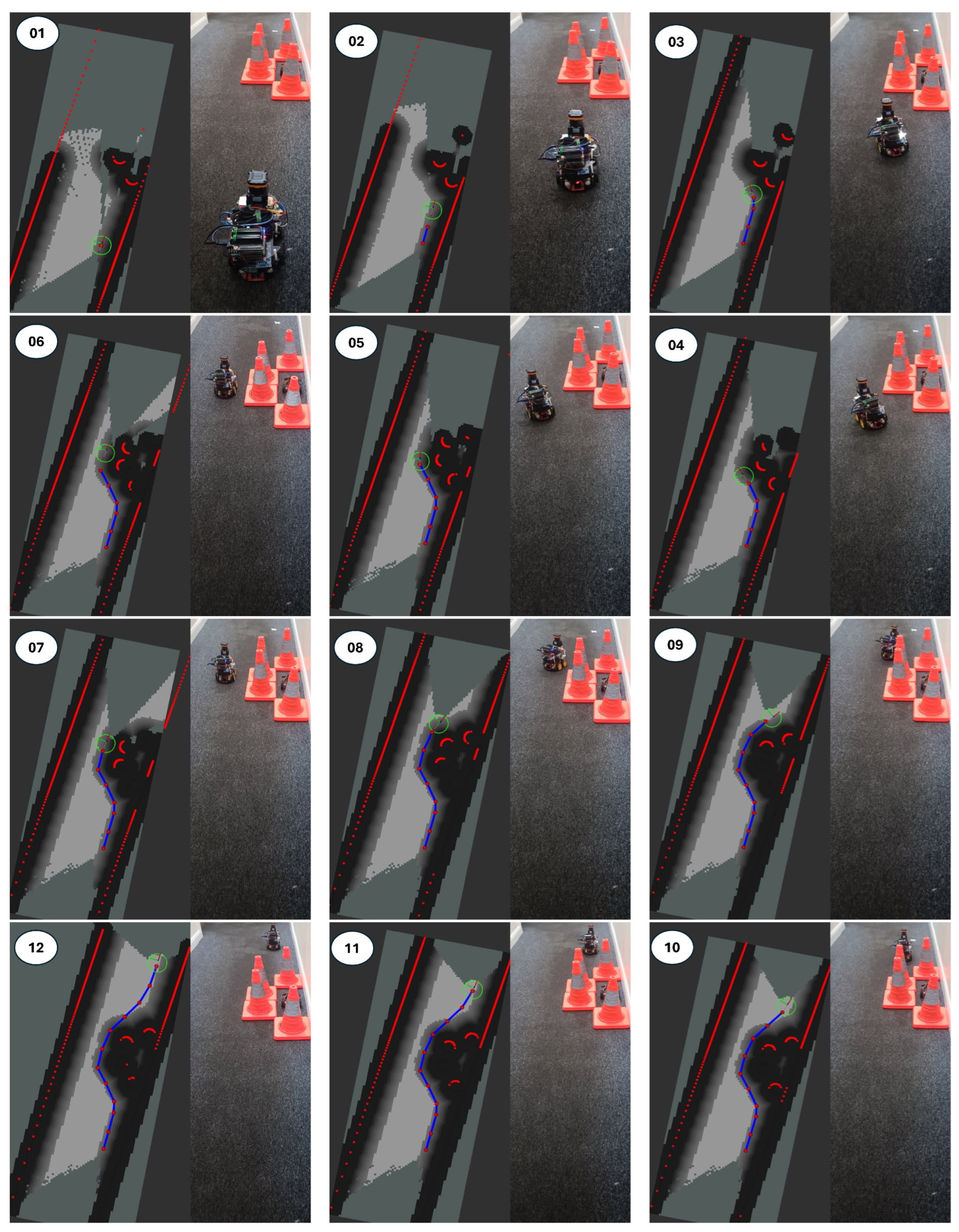
Figure 13 and Figure 14 show a sample of the step-by-step results of the path followed by the car using the proposed ADS structure and the RDE algorithm in the chicanes and road works overtaking scenarios. Each frame shows the vehicle in real time alongside its corresponding RViz environment visualization.

The path is indicated by a blue line, divided by equally spaced red circles generated by RViz during path construction. The real-time laser scan is indicated by red boundaries that surround the front side of obstacles facing the LiDAR at each time step. The car’s current location is marked by a green circle, with a frame attached to its center showing the vehicle’s current orientation.

As the car moves, the surrounding environment is incrementally mapped using the Hector SLAM node from frame 1 to frame 12. The occupancy grid assigns cost values to each cell, indicated by different colors. The purple color marks obstacle boundaries with the highest cost of 254, representing a 100% collision risk. Cyan indicates inflated zones that the car’s center cannot enter. Areas near obstacles range from red to dark blue (costs 253 to 1), within which the robot is allowed to navigate. Black regions denote free space with zero cost, indicating safe traversal zones.

These results demonstrate that the vehicle successfully navigated the chicanes and roadworks in a collision-free manner, as generated by the proposed ADS system, proving the perfect integration between all the nodes. The following section discusses the statistical analysis of the results for four state-of-the-art path-planning algorithms.

8. Results Statistical Analysis and Discussion

This section compares the proposed ROS-based Differential Evolution (RDE) planner against four conventional path-planning algorithms commonly used within the ROS system: A*, RRT, A*+TEB, and DWA. The aim is to assess the practical performance of RDE relative to these baseline planners in terms of path cost and statistical significance across real-world scenarios.

8.1. Comparison Setup and Local Planning Configuration

All algorithms are deployed in a local planning configuration within the same ROS architecture to ensure a fair and consistent comparison. Fixed short-range goals are assigned in each scenario, and each planner generates paths based on real-time LiDAR-derived occupancy maps from Hector SLAM. While A* is traditionally used for global planning, it is executed in our setup using local SLAM maps to reach short-distance goals without relying on pre-loaded global maps or predefined routes. This uniform design ensures that each algorithm operates under identical conditions and inputs.

Using the 4WD car platform, all algorithms are tested across six chicane driving scenarios. For each planner, 20 independent runs are conducted per scenario. The parameter settings for all planners are detailed in

Table 5. Summary of parameter settings for path-planning algorithms.

Algorithm	Parameters
A*	Grid resolution = 0.01
RRT	Step size = 0.01
	$v_{max}$ = 0.4, $a_{max}$ = 0.5, Safety margin = 0.25
A*TEB [46]	Weight length = 30, Grid resolution = 0.01
	$v_{max}$ = 0.4, $v_{min}$ = 0, linear velocity resolution = 0.01
DWA [96,97]	${\omega }_{max}$ = $\pi /4$, ${\omega }_{min}$ = $-\pi /4$, angular velocity resolution = 0.1, $\Delta t$ = 0.1
RDE	$NP=30$, F = 0.5, $CR$ = 0.5

. All algorithms are configured to terminate upon finding their first valid solution, while the RDE planner is allowed to run up to a maximum of $10,000\times n_{obst}$ function evaluations, where $n_{obst}$ represents the number of obstacle clusters detected by the DBSCAN algorithm. The resulting path costs are recorded as previously described, and statistical analysis is performed to evaluate comparative effectiveness and significance.

8.2. Results Collection and Visualization

Table 6. Best, worst, median, mean, and SD path cost results of all the algorithms across the 20 experiments for the scenarios (S1–S6).

S No.	Alg.	Best	Worst	Median	Mean	SD
S1	A*	2.00000000 ×${10}^2$	2.00000000 ×${10}^2$	2.00000000 $\times {10}^2$	2.00000000 $\times {10}^2$	0.00000000
	A*TEB	3.62384274 ×${10}^2$	3.62384274 ×${10}^2$	3.62384274 ×${10}^2$	3.62384274 ×${10}^2$	1.16640234 ×${10}^{-13}$
	RRT	2.00116704 ×${10}^2$	2.08740222 ×${10}^2$	2.01575938 ×${10}^2$	2.02458382 ×${10}^2$	2.15278122
	DWA	2.01047468 ×${10}^2$	2.01047468 ×${10}^2$	2.01047468 ×${10}^2$	2.01047468 ×${10}^2$	8.74801758 ×${10}^{-14}$
	RDE	2.00000000 ×${10}^2$	2.00000000 ×${10}^2$	2.00000000 $\times {10}^2$	2.00000000 $\times {10}^2$	0.00000000
S2	A*	8.75192075 × 10	8.75192075 × 10	8.75192075 × 10	8.75192075 × 10	0.00000000
	A*TEB	4.73667614 ×${10}^2$	4.73667614 ×${10}^2$	4.73667614 ×${10}^2$	4.73667614 ×${10}^2$	0.00000000
	RRT	8.52189202 × 10	1.19273804 ×${10}^2$	9.70616612 × 10	9.83924551 × 10	9.73163601
	DWA	9.28122347 × 10	9.28122347 × 10	9.28122347 × 10	9.28122347 × 10	2.91600586 ×${10}^{-14}$
	RDE	8.15317851 × 10	9.30635455 × 10	8.15317851 $\times 10$	8.21088853 $\times 10$	2.57846002
S3	A*	1.60194616 ×${10}^2$	1.60194616 ×${10}^2$	1.60194616 ×${10}^2$	1.60194616 ×${10}^2$	5.83201172 ×${10}^{-14}$
	A*TEB	7.18529285 ×${10}^2$	7.18529285 ×${10}^2$	7.18529285 ×${10}^2$	7.18529285 ×${10}^2$	2.33280469 ×${10}^{-13}$
	RRT	1.58055638 ×${10}^2$	1.82707339 ×${10}^2$	1.67118392 ×${10}^2$	1.67918799 ×${10}^2$	5.79856369
	DWA	1.63021900 ×${10}^2$	1.63021900 ×${10}^2$	1.63021900 ×${10}^2$	1.63021900 ×${10}^2$	5.83201172 ×${10}^{-14}$
	RDE	1.52676247 ×${10}^2$	1.52680889 ×${10}^2$	1.52676551 $\times {10}^2$	1.52677171 $\times {10}^2$	1.33552752 ×${10}^{-3}$
S4	A*	1.47475290 ×${10}^2$	1.47475290 ×${10}^2$	1.47475290 ×${10}^2$	1.47475290 ×${10}^2$	2.91600586 ×${10}^{-14}$
	A*TEB	1.07240462 ×${10}^3$	1.07240462 ×${10}^3$	1.07240462 ×${10}^3$	1.07240462 ×${10}^3$	2.33280469 ×${10}^{-13}$
	RRT	1.52826598 ×${10}^2$	1.76183628 ×${10}^2$	1.61016604 ×${10}^2$	1.61394440 ×${10}^2$	7.47421701
	DWA	1.69999293 ×${10}^2$	1.69999293 ×${10}^2$	1.69999293 ×${10}^2$	1.69999293 ×${10}^2$	2.91600586 ×${10}^{-14}$
	RDE	1.49785795 ×${10}^2$	1.49910983 ×${10}^2$	1.49793129 ×${10}^2$	1.49802956 ×${10}^2$	3.15616530 ×${10}^{-2}$
S5	A*	2.17247995 ×${10}^2$	2.17247995 ×${10}^2$	2.17247995 ×${10}^2$	2.17247995 ×${10}^2$	2.91600586 ×${10}^{-14}$
	A*TEB	8.33081518 ×${10}^3$	8.33081518 ×${10}^3$	8.33081518 ×${10}^3$	8.33081518 ×${10}^3$	0.00000000
	RRT	2.20839573 ×${10}^2$	2.50735916 ×${10}^2$	2.28663314 ×${10}^2$	2.31625135 ×${10}^2$	8.12402140
	DWA	2.29383191 ×${10}^2$	2.29383191 ×${10}^2$	2.29383191 ×${10}^2$	2.29383191 ×${10}^2$	1.16640234 ×${10}^{-13}$
	RDE	2.08182454 ×${10}^2$	2.08201368 ×${10}^2$	2.08185161 $\times {10}^2$	2.08186998 $\times {10}^2$	5.06874043 ×${10}^{-3}$
S6	A*	2.57185725 ×${10}^2$	2.57185725 ×${10}^2$	2.57185725 ×${10}^2$	2.57185725 ×${10}^2$	0.00000000
	A*TEB	1.47008696 ×${10}^3$	1.47008696 ×${10}^3$	1.47008696 ×${10}^3$	1.47008696 ×${10}^3$	4.66560938 ×${10}^{-13}$
	RRT	2.56951451 ×${10}^2$	2.78581854 ×${10}^2$	2.64370048 ×${10}^2$	2.65120604 ×${10}^2$	5.81853033
	DWA	2.61966070 ×${10}^2$	2.61966070 ×${10}^2$	2.61966070 ×${10}^2$	2.61966070 ×${10}^2$	5.83201172 ×${10}^{-14}$
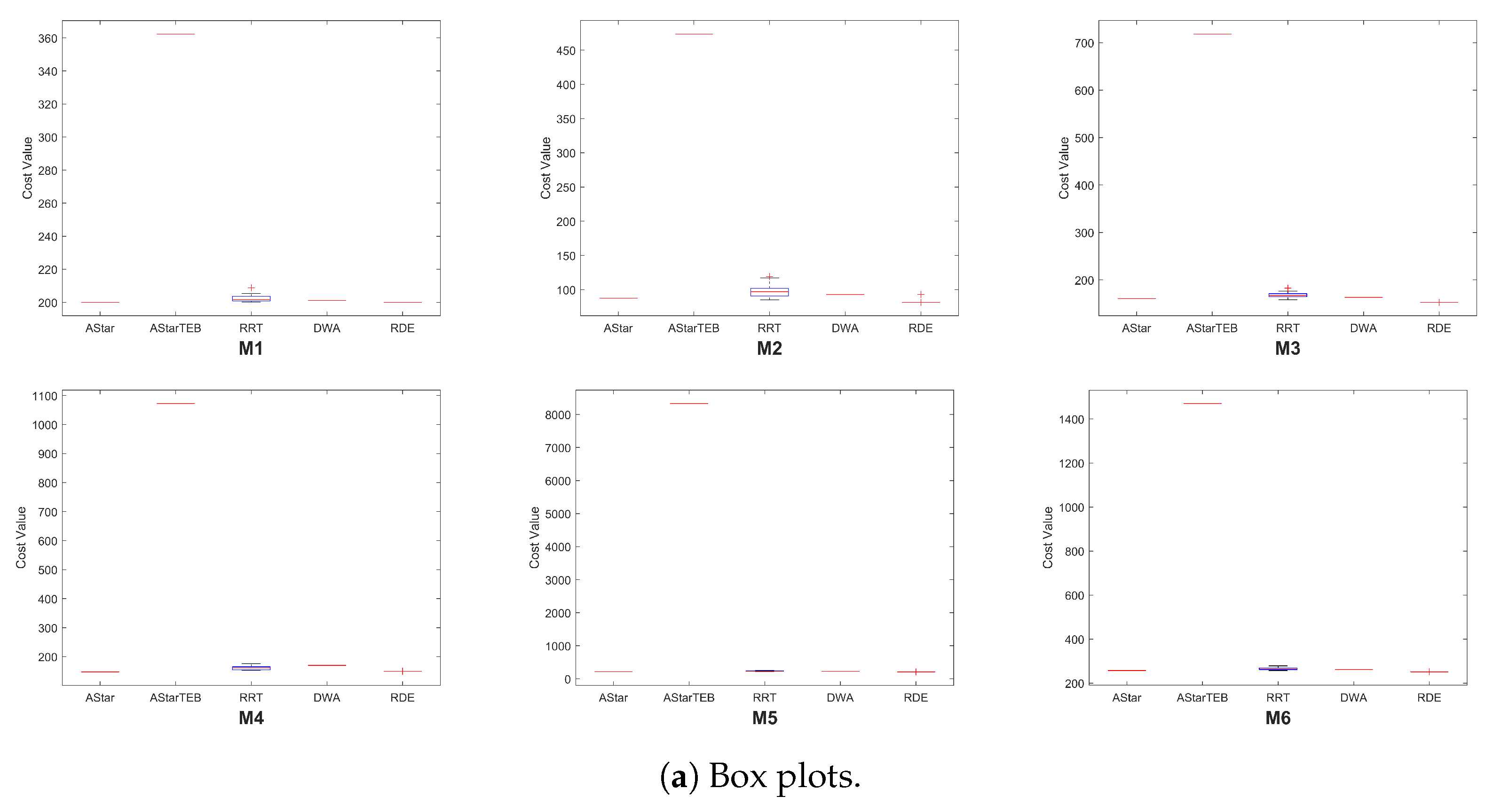
	RDE	2.51004800 ×${10}^2$	2.52346676 ×${10}^2$	2.51005463 $\times {10}^2$	2.51083162 $\times {10}^2$	2.98022348 ×${10}^{-1}$

presents the best, worst, median, mean, and SD of the path costs obtained over 20 runs for each algorithm across the six chicane driving scenarios. The distribution of these results is visualized using box plots in Figure 15a and violin plots in Figure 15b. A compact and low-positioned box indicates both low cost and high consistency across runs in the box plots. The A*TEB algorithm exhibited significantly higher path costs than the other planners, resulting in its exclusion from the violin plots to enhance the visibility of the other algorithms’ distributions.

The results show that the proposed RDE consistently has compact, low-positioned boxes in all scenarios, indicating low path cost and high repeatability. The only exception is Scenario 4, where the A* algorithm has less path cost than RDE. In contrast, the RRT displays the widest boxes and violin shapes, indicating non-repeatable results and a lack of consistency across runs. Compared to A*, A*TEB, DWA, and RRT, the RDE planner offers the most reliable and efficient path-planning performance in the tested scenarios.

8.3. Statistical Analysis Results

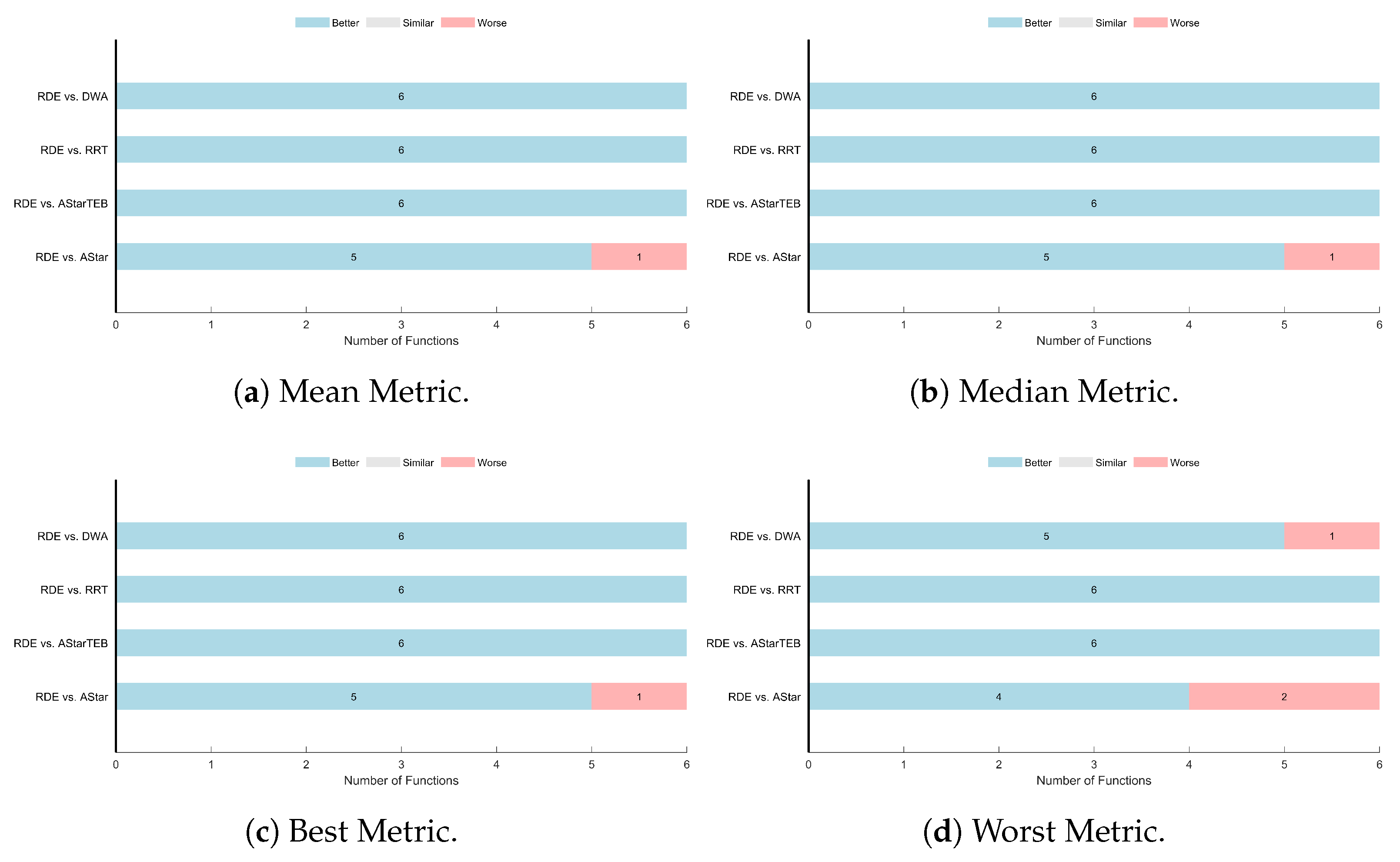
Figure 16 and

Table 7. Statistical analysis of all the experiments for all six scenarios for all the path-planning algorithms: A*, A*TEB, RRT, DWA, and RDE. RDE is the reference algorithm in all comparisons, and thus the Wilcoxon test is not applicable (NA) for RDE as it cannot be compared against itself. ‘+’ means the number of scenarios in which the RDE is better, and ‘=’ means draw. The level of significance $\alpha$ is 0.05. The results are significant if p-value $<\alpha$. In the Friedman test, the best algorithm is the one with the minimum mean rank.

Metric	Alg.	Wilcoxon	Friedman Test
	Name	Test	SumRanks	MeanRanks	Rank	p-Value
Mean	A*	+5/=0/−1	11	1.83333333	2	0.00014760
	A*TEB	+6/=0/−0	30	5.00000000	5
	RRT	+6/=0/−0	23	3.83333333	4
	DWA	+6/=0/−0	19	3.16666667	3
	RDE	NA	7	1.16666667	1
Median	A*	+5/=0/−1	11	1.83333333	2	0.00017735
	A*TEB	+6/=0/−0	30	5.00000000	5
	RRT	+6/=0/−0	22	3.66666667	4
	DWA	+6/=0/−0	20	3.33333333	3
	RDE	NA	7	1.16666667	1
Worst	A*	+4/=0/−2	10	1.66666667	2	0.00022646
	A*TEB	+6/=0/−0	30	5.00000000	5
	RRT	+6/=0/−0	24	4.00000000	4
	DWA	+5/=0/−1	17	2.83333333	3
	RDE	NA	9	1.50000000	1
Best	A*	+5/=0/−1	14	2.33333333	2	0.00022646
	A*TEB	+6/=0/−0	30	5.00000000	5
	RRT	+6/=0/−0	15	2.50000000	3
	DWA	+6/=0/−0	24	4.00000000	4
	RDE	NA	7	1.16666667	1

present the results of the Wilcoxon Signed-Rank test and the Friedman test for all evaluated cost metrics. The Wilcoxon Signed-Rank test is conducted to evaluate the pairwise statistical significance of the RDE algorithm against each competing method across all six driving scenarios. For the mean, median, and best metrics, RDE outperformed A* in 5 out of 6 scenarios and outperformed A*TEB, RRT, and DWA in all scenarios. For the worst cost metric, RDE outperformed A* in 4 scenarios, DWA in 5, and A*TEB and RRT in all 6 scenarios. These consistent wins highlight the superior reliability and performance of RDE across different statistical measures.

The Friedman test is used to compare the overall rankings of the algorithms across the six scenarios. For all cost metrics (mean, median, worst, and best), RDE achieved the top rank (Rank 1). The corresponding mean ranks for RDE were the lowest among all planners: 1.17 (mean), 1.17 (median), 1.50 (worst), and 1.17 (best). In contrast, A*TEB consistently ranked lowest, with a mean rank of 5.00. The p-values for all metrics were below the significance threshold ($\alpha =0.05$), confirming that the observed differences among the algorithms are statistically significant.

9. Computational Complexity Analysis

This section analyzes the computational complexity of the proposed RDE-based planning node and compares it against traditional A*+DWA/TEB pipelines in both theoretical and practical contexts.

9.1. Asymptotic Complexity Comparison

The overall computational complexity of the proposed ROS-based path-planning node is primarily governed by the DE optimization process, but it also involves several preprocessing stages, including map boundary extraction, LiDAR-based goal determination, cost evaluation, and DBSCAN-based obstacle clustering. The DE component, which dominates the runtime, has a complexity of $\mathcal{O}(N_p·n_{obst}·T)$, where $N_p$ is the population size, $n_{obst}$ represents the number of DE decision variables (scaled to the number of clustered obstacles), and T is the maximum number of DE iterations.

The clustering phase using DBSCAN operates on a set of obstacle points N and has a worst-case complexity of $\mathcal{O}\left(N^2\right)$, although efficient indexing (KD-trees) typically reduces this to near-linear time. Additionally, higher-resolution maps (smaller $M_{res}$) increase the cost of cell indexing and penalty calculations. However, the proposed node constrains all operations within a dynamic local field defined by the LiDAR range, which is typically constrained to 30 m, reducing unnecessary computation.

In contrast, traditional pipelines combine A* for global planning with DWA or TEB for local planning. A* requires full-map traversal with a time complexity of $\mathcal{O}(MlogM)$, where M is the number of traversable cells, making it inefficient for large or dynamic environments. The local planner TEB incurs high overhead due to continuous trajectory optimization and constraint solving, with worst-case time complexity up to $\mathcal{O}\left(k^3\right)$, where k is the number of trajectory states [45]. DWA, while faster, relies on dense velocity sampling and repeated trajectory rollouts, often reaching $\mathcal{O}(n_v·n_{\theta }·n_t)$, where $n_v$ and $n_{\theta }$ are sampled linear and angular velocities, and $n_t$ is the time horizon steps [98]. These methods depend on fixed-resolution grids and are less adaptive to localized changes or sensor-driven updates.

In summary, the proposed RDE node achieves a total computational complexity of $\mathcal{O}(N_p·n_{obst}·T+N)$, compared to $\mathcal{O}(MlogM+n_v·n_{\theta }·n_t)$ for the A*+DWA pipeline and $\mathcal{O}(MlogM+k^3)$ for A*+TEB. By unifying global and local planning within a single DE-based optimization loop and operating entirely on real-time LiDAR occupancy data, RDE avoids global traversal and velocity discretization, offering better scalability and responsiveness in dynamic environments.

9.2. Practical Time Complexity Analysis

The time complexity metrics $T_0$, $T_1$, $T_2$, and $T_3$, previously introduced for benchmarking CEC2020 functions, are analogously applied here to evaluate the computational efficiency of each planner in real driving scenarios. Specifically, $T_0$ captures the baseline computational speed of the onboard controller (Raspberry Pi). A fixed arithmetic-intensive code is run on the controller in isolation for a large number of iterations (200,000 in our study), measuring the total time with a built-in timing function, yielding a $T_0=0.0029934$.

The metric $T_1$ represents the time consumed by environment handling alone, such as sensor reading (LiDAR and IMU), basic data logging, and trivial motion commands, without executing the main path-planning algorithm. For each scenario, we disabled the advanced planner node (e.g., RDE). We allowed the robot to remain idle, recording the total execution time over a fixed number of iterations, averaging them across scenarios to obtain $T_1=10.56$. The metric $T_2$ measures the full execution time, including the path-planning node. The final metric, $T_3=(T_2-T_1)/T_0$, normalizes the net planning overhead by the hardware’s baseline speed, providing a hardware-independent comparison.

Table 8. Time complexity results for all algorithms across all scenarios.

Algorithm	T0	T1	T2	T3	Rank
A*	0.00299340	10.56405612	147.16016833	45,632.42874880	3
A*TEB	0.00299340	10.56405612	173.68609014	54,493.89792000	5
RRT	0.00299340	10.56405612	56.72592000	15,421.21463330	2
DWA	0.00299340	10.56405612	147.38945167	45,709.02503842	4
RDE	0.00299340	10.56405612	38.12321333	9206.64034765	1

reports these metrics across all six driving scenarios. The proposed RDE algorithm consistently achieves the lowest $T_3$ value (9206.64), indicating the most efficient computational performance among all methods. RRT ranks second (15,421.21), followed by A* (45,632.43), DWA (45,709.03), and A*TEB (54,493.90). These results demonstrate that RDE not only excels in planning accuracy but also minimizes computational load, which represents an essential factor for energy-efficient operation in embedded or battery-powered autonomous vehicles.

10. Deployment Extensions for Outdoor and Dynamic Environments

This section presents a set of practical considerations and implementation guidelines for extending the proposed RDE-based local planning framework from indoor validation to outdoor road navigation. It also outlines how it can be adapted to handle dynamic obstacles in real-world scenarios.

10.1. Deployment Considerations for Outdoor and Road-Based Navigation

While the current validation was conducted using an indoor 4WD robot, the core architecture of the proposed RDE-based local planner is designed to be directly transferable to outdoor road scenarios. In such scenarios, the global navigation route is typically generated from GPS or high-level mission planners, which provide sequential waypoints along the road network. These GPS-derived waypoints can seamlessly replace the dynamically generated short-range goals used in the indoor experiments. Once received, each waypoint becomes the target input for the RDE local planner, which then computes a smooth, collision-free path segment using real-time LiDAR data.

Additionally, the system can be extended with a vision-based perception layer that uses camera inputs to recognize road lanes, traffic signs, and dynamic road agents. These perception outputs can be incorporated into the local planning process either by constraining the search space (e.g., enforcing lane boundaries) or influencing decision-making logic (e.g., yielding or stopping). For instance, a detected lane centerline can limit the feasible region where RDE explores new paths, ensuring road compliance. This hybrid structure mirrors real-world autonomous driving architectures, where GPS provides long-range routing and vision sensors support short-range planning.

The control and Arduino nodes are designed to accommodate both configurations (4WD and Ackermann) with minimal modifications to support outdoor vehicle scenarios where Ackermann steering is more common than 4WD mechanisms. Furthermore, the hardware controllers will be upgraded to handle higher power demands typical of road vehicles. For example, low-power modules such as the LM358 motor driver will be replaced with more robust controllers like the Cytron MD30 series, and the control units themselves will be scaled accordingly to ensure stable operation under real-world driving conditions.

10.2. Handling Dynamic Obstacles

Although the driving scenarios in this study involve static obstacles, the software stack is already configured for dynamic environments. The Hokuyo UTM-30LX delivers range scans at $40\mathrm{Hz}$, while the RDE optimizer is invoked after every fifth scan, resulting in an effective replanning rate of $8\mathrm{Hz}$ ($125\mathrm{ms}$ cycle). This duration is significantly longer than the measured optimization time of $39\mathrm{ms}$, ensuring that each planning cycle is completed before the next trigger. Therefore, pedestrians or vehicles that cross the laser field are interpreted as transient obstacles in the updated occupancy grid. The RDE planner then immediately provides a collision-free path that reflects recent motion updates, allowing the vehicle to avoid the obstacle in the next planning round.

While dynamic obstacle testing lies beyond the current experimental scope, the proposed framework can be extended to handle such cases using the following two enhancements. First, a lightweight strategy inspired by Dynamic Occupancy Grid Mapping (DOGM) can be incorporated to track short-term occupancy history across successive scans [99]. Grid cells that alternate frequently between free and occupied states over a brief window (e.g., 10 frames) are flagged as potentially dynamic. These flagged cells are grouped into clusters, and if a cluster’s centroid shifts beyond a defined threshold (e.g., 15–20 cm), it is identified as a dynamic object. If any such cluster intersects the current path, an internal flag triggers immediate replanning. This mechanism requires no additional ROS topics and integrates efficiently into the existing architecture.

Second, the system can benefit from incorporating localized frontier-led exploration, as inspired by the dynamic frontier-led swarming approach proposed by Tran et al. [100]. While originally developed for multi-robot systems, a simplified adaptation can be applied to a single robot by periodically re-evaluating unexplored or recently cleared map frontiers. These frontiers can be prioritized in the RDE waypoint-generation phase. Then, the robot can adjust its path based on the dynamically emerging free space.

Although the current system has been validated indoors using a 4WD robot in static environments, its modular design allows straightforward adaptation to outdoor, real-world conditions. With minor software adjustments and hardware upgrades, the same RDE-based framework can be deployed in full-scale autonomous vehicles for dynamic, road-based navigation.

11. Conclusions

This study presents a modular ROS-based autonomous driving system comprising eight integrated nodes, each dedicated to a specific task within the ADS pipeline. The system features enhanced path-planning and control capabilities, integrating LiDAR-based Hector SLAM for real-time mapping, an Extended Kalman Filter (EKF) for robust localization, and a Differential Evolution (DE)-based optimizer for path planning to ensure adaptive and efficient navigation.

In the path-planning node, a ROS-based Differential Evolution (RDE) algorithm is implemented with a dynamic cost function that estimates the path cost based on Hector-SLAM mapping and DBSCAN clustering. The goal point is dynamically allocated according to LiDAR range and search space boundaries, ensuring adaptability in real-world environments. Unlike conventional planners that generate motor velocities, the RDE algorithm generates Cartesian coordinates, enhancing generalization and cross-platform compatibility.

In the control node, a modified pure-pursuit algorithm translates waypoints from the path planner into motor velocity commands for the Arduino node, considering the drift angle to ensure accurate trajectory execution. The DE algorithm dynamically adjusts the PID controller gains, optimizing motor speed control for smooth vehicle handling. With minor modifications in the control node, this architecture can be adapted and deployed across various vehicle platforms.

Extensive simulations and real-world experiments validated the system’s performance, demonstrating its ability to generate collision-free paths with reduced path length and enhanced execution efficiency. Comparative evaluations revealed that the proposed RDE method outperformed state-of-the-art planners, such as A*, RRT, DWA, and A*TEB. RDE ranked first in the Friedman test, achieving a significance level of 0.05, with better convergence and lower computational overhead.

In the future, the proposed system could be extended to support various vehicle architectures, including Omni-wheel (Mecanum) steering systems, to evaluate its adaptability across different mobility platforms. Additionally, other meta-heuristic optimization algorithms could be implemented within the path-planning node to compare their performance. The perception layer could also be expanded by incorporating an RGB camera and deep learning-based computer vision techniques for object-recognition tasks. Overall, the proposed ADS framework has demonstrated its efficiency, modularity, and flexibility, and future research could focus on its improvement.

References

- Marchand, R. The Designers Go to the Fair II: Norman Bel Geddes, The General Motors “Futurama,” and the Visit to the Factory Transformed. Des. Issues 1992, 8, 23–40. [Google Scholar] [CrossRef]
- Buehler, M.; Iagnemma, K.; Singh, S. The DARPA Urban Challenge: Autonomous Vehicles in City Traffic; Springer Science & Business Media: Berlin/Heidelberg, Germany, 2009; Volume 56. [Google Scholar]
- Velasco-Hernandez, G.; Yeong, D.J.; Barry, J.; Walsh, J. Autonomous driving architectures, perception and data fusion: A review. In Proceedings of the 2020 IEEE 16th International Conference on Intelligent Computer Communication and Processing (ICCP), Cluj-Napoca, Romania, 3–5 September 2020; pp. 315–321. [Google Scholar]
- Wong, K.; Gu, Y.; Kamijo, S. Mapping for autonomous driving: Opportunities and challenges. IEEE Intell. Transp. Syst. Mag. 2020, 13, 91–106. [Google Scholar] [CrossRef]
- Parekh, D.; Poddar, N.; Rajpurkar, A.; Chahal, M.; Kumar, N.; Joshi, G.P.; Cho, W. A review on autonomous vehicles: Progress, methods and challenges. Electronics 2022, 11, 2162. [Google Scholar] [CrossRef]
- Shekh, M.; Umrao, O.; Singh, D. Kinematic Analysis of Steering Mechanism: A Review. In Proceedings of the International Conference in Mechanical and Energy Technology: ICMET 2019, Greater Noida, India, 7–8 November 2019; Springer: Berlin/Heidelberg, Germany, 2020; pp. 529–540. [Google Scholar]
- Saleem, H.; Riaz, F.; Mostarda, L.; Niazi, M.A.; Rafiq, A.; Saeed, S. Steering angle prediction techniques for autonomous ground vehicles: A review. IEEE Access 2021, 9, 78567–78585. [Google Scholar] [CrossRef]
- Quigley, M.; Conley, K.; Gerkey, B.; Faust, J.; Foote, T.; Leibs, J.; Berger, E.; Wheeler, R.; Ng, A.Y. ROS: An open-source Robot Operating System. In Proceedings of the ICRA Workshop on Open Source Software, Kobe, Japan, 12–17 May 2009; Volume 3, p. 5. [Google Scholar]
- Ali, S.; Jalal, A.; Alatiyyah, M.H.; Alnowaiser, K.; Park, J. Vehicle detection and tracking in UAV imagery via YOLOv3 and Kalman filter. Comput. Mater. Contin. 2023, 76, 1249–1265. [Google Scholar] [CrossRef]
- Jin, Q.; Liu, Y.; Man, Y.; Li, F. Visual slam with rgb-d cameras. In Proceedings of the 2019 Chinese Control Conference (CCC), Guangzhou, China, 27–30 July 2019; pp. 4072–4077. [Google Scholar]
- Hong, Z.; Petillot, Y.; Wallace, A.; Wang, S. RadarSLAM: A robust simultaneous localization and mapping system for all weather conditions. Int. J. Robot. Res. 2022, 41, 519–542. [Google Scholar] [CrossRef]
- Burnett, K.; Wu, Y.; Yoon, D.J.; Schoellig, A.P.; Barfoot, T.D. Are we ready for radar to replace lidar in all-weather mapping and localization? IEEE Robot. Autom. Lett. 2022, 7, 10328–10335. [Google Scholar] [CrossRef]
- Purnama, H.S.; Sutikno, T.; Alavandar, S.; Subrata, A.C. Intelligent control strategies for tuning PID of speed control of DC motor—A review. In Proceedings of the 2019 IEEE Conference on Energy Conversion (CENCON), Yogyakarta, Indonesia, 16–17 October 2019; pp. 24–30. [Google Scholar]
- Sridhar, H.; Hemanth, P.; Pavitra; Soumya, H.; Joshi, B.G. Speed control of BLDC motor using soft computing technique. In Proceedings of the 2020 International Conference on Smart Electronics and Communication (ICOSEC), Trichy, India, 10–12 September 2020; pp. 1162–1168. [Google Scholar]
- Chitta, S.; Marder-Eppstein, E.; Meeussen, W.; Pradeep, V.; Tsouroukdissian, A.R.; Bohren, J.; Coleman, D.; Magyar, B.; Raiola, G.; Lüdtke, M.; et al. ros_control: A generic and simple control framework for ROS. J. Open Source Softw. 2017, 2, 456. [Google Scholar] [CrossRef]
- Reda, M.; Onsy, A.; Haikal, A.Y.; Ghanbari, A. Path-planning algorithms in the autonomous driving system: A comprehensive review. Robot. Auton. Syst. 2024, 174, 104630. [Google Scholar] [CrossRef]
- Foead, D.; Ghifari, A.; Kusuma, M.B.; Hanafiah, N.; Gunawan, E. A systematic literature review of A* pathfinding. Procedia Comput. Sci. 2021, 179, 507–514. [Google Scholar] [CrossRef]
- Gautam, S.C.; Lim, J.; Jaar, B.G. Complications associated with continuous RRT. Kidney360 2022, 3, 1980–1990. [Google Scholar] [CrossRef]
- Kobayashi, M.; Motoi, N. Local path planning: Dynamic window approach with virtual manipulators considering dynamic obstacles. IEEE Access 2022, 10, 17018–17029. [Google Scholar] [CrossRef]
- Heidari, A.A.; Mirjalili, S.; Faris, H.; Aljarah, I.; Mafarja, M.; Chen, H. Harris hawks optimization: Algorithm and applications. Future Gener. Comput. Syst. 2019, 97, 849–872. [Google Scholar] [CrossRef]
- Simon, D. Biogeography-based optimization. IEEE Trans. Evol. Comput. 2008, 12, 702–713. [Google Scholar] [CrossRef]
- Wang, Y.; Liu, Z.; Zuo, Z.; Ll, Z. Local path planning of autonomous vehicles based on A* algorithm with equal-step sampling. In Proceedings of the 2018 37th Chinese Control Conference (CCC), Wuhan, China, 25–27 July 2018; pp. 7828–7833. [Google Scholar]
- Udomsil, R.; Sangpet, T.; Sapsaman, T. Environment generation from real map to investigate path planning and obstacle avoidance algorithm for electric vehicle. In Proceedings of the 2019 Research, Invention, and Innovation Congress (RI2C), Bangkok, Thailand, 11–13 December 2019; pp. 1–5. [Google Scholar]
- Zhong, X.; Tian, J.; Hu, H.; Peng, X. Hybrid path planning based on safe A* algorithm and adaptive window approach for mobile robot in large-scale dynamic environment. J. Intell. Robot. Syst. 2020, 99, 65–77. [Google Scholar] [CrossRef]
- Li, B.; Dong, C.; Chen, Q.; Mu, Y.; Fan, Z.; Wang, Q.; Chen, X. Path planning of mobile robots based on an improved A* algorithm. In Proceedings of the 2020 4th High Performance Computing and Cluster Technologies Conference & 2020 3rd International Conference on Big Data and Artificial Intelligence, Qingdao, China, 3–6 July 2020; pp. 49–53. [Google Scholar]
- Zhang, D.; Chen, C.; Zhang, G. AGV path planning based on improved A-star algorithm. In Proceedings of the 2024 IEEE 7th Advanced Information Technology, Electronic and Automation Control Conference (IAEAC), Chongqing, China, 15–17 March 2024; Volume 7, pp. 1590–1595. [Google Scholar]
- Thoresen, M.; Nielsen, N.H.; Mathiassen, K.; Pettersen, K.Y. Path planning for UGVs based on traversability hybrid A. IEEE Robot. Autom. Lett. 2021, 6, 1216–1223. [Google Scholar] [CrossRef]
- Liu, T.; Zhang, J. An improved path-planning algorithm based on fuel consumption. J. Supercomput. 2022, 78, 12973–13003. [Google Scholar] [CrossRef]
- González, D.; Pérez, J.; Milanés, V.; Nashashibi, F. A review of motion planning techniques for automated vehicles. IEEE Trans. Intell. Transp. Syst. 2015, 17, 1135–1145. [Google Scholar] [CrossRef]
- Lu, D.V.; Ferguson, M.; Hoy, A. Global_Planner: A Fast Interpolated Global Path Planner for ROS Navigation. 2021. Available online: http://wiki.ros.org/global_planner (accessed on 8 July 2025).
- Wang, J.; Wu, S.; Li, H.; Zou, J. Path planning combining improved rapidly-exploring random trees with dynamic window approach in ROS. In Proceedings of the 2018 13th IEEE Conference on Industrial Electronics and Applications (ICIEA), Wuhan, China, 31 May–2 June 2018; pp. 1296–1301. [Google Scholar]
- Chen, J.; Liang, J.; Tong, Y. Path Planning of Mobile Robot Based on Improved Differential Evolution Algorithm. In Proceedings of the 2020 16th International Conference on Control, Automation, Robotics and Vision (ICARCV), Shenzhen, China, 13–15 December 2020; pp. 811–816. [Google Scholar]
- Hu, B.; Cao, Z.; Zhou, M. An efficient RRT-based framework for planning short and smooth wheeled robot motion under kinodynamic constraints. IEEE Trans. Ind. Electron. 2020, 68, 3292–3302. [Google Scholar] [CrossRef]
- Niu, C.; Li, A.; Huang, X.; Xu, C. Research on Intelligent Vehicle Path Planning Method Based on Improved RRT Algorithm. In Proceedings of the 2021 Global Reliability and Prognostics and Health Management (PHM-Nanjing), Yantai, China, 13–16 October 2022; pp. 1–7. [Google Scholar]
- Shi, P.; Liu, Z.; Liu, G. Local path planning of unmanned vehicles based on improved RRT algorithm. In Proceedings of the the 2022 4th Asia Pacific Information Technology Conference, Virtual, 14–16 January 2022; pp. 231–239. [Google Scholar]
- Chen, R.; Hu, J.; Xu, W. An RRT-Dijkstra-based path planning strategy for autonomous vehicles. Appl. Sci. 2022, 12, 11982. [Google Scholar] [CrossRef]
- Yang, G.; Yao, Y. Vehicle local path planning and time consistency of unmanned driving system based on convolutional neural network. Neural Comput. Appl. 2022, 34, 12385–12398. [Google Scholar] [CrossRef]
- Zhang, X.; Zhu, T.; Xu, Y.; Liu, H.; Liu, F. Local Path Planning of the Autonomous Vehicle Based on Adaptive Improved RRT Algorithm in Certain Lane Environments. Actuators 2022, 11, 109. [Google Scholar] [CrossRef]
- Mao, S.; Yang, P.; Gao, D.; Bao, C.; Wang, Z. A Motion Planning Method for Unmanned Surface Vehicle Based on Improved RRT Algorithm. J. Mar. Sci. Eng. 2023, 11, 687. [Google Scholar] [CrossRef]
- Marder-Eppstein, E.; Lu, D.V.; Ferguson, M.; Hoy, A. Dwa_Local_Planner: Dynamic Window Approach for Local Navigation. 2020. Available online: http://wiki.ros.org/dwa_local_planner (accessed on 8 July 2025).
- Zhang, F.; Li, N.; Xue, T.; Zhu, Y.; Yuan, R.; Fu, Y. An improved dynamic window approach integrated global path planning. In Proceedings of the 2019 IEEE International Conference on Robotics and Biomimetics (ROBIO), Dali, China, 6–8 December 2019; pp. 2873–2878. [Google Scholar]
- Liu, L.-S.; Lin, J.-F.; Yao, J.-X.; He, D.-W.; Zheng, J.-S.; Huang, J.; Shi, P. Path planning for smart car based on Dijkstra algorithm and dynamic window approach. Wirel. Commun. Mob. Comput. 2021, 2021, 8881684. [Google Scholar] [CrossRef]
- hua Zhang, J.; Feng, Q.; di Zhao, A.; He, W.; Hao, X. Local path planning of mobile robot based on self-adaptive dynamic window approach. J. Phys. Conf. Ser. 2021, 1905, 012019. [Google Scholar] [CrossRef]
- Fox, D.; Burgard, W.; Thrun, S. The dynamic window approach to collision avoidance. IEEE Robot. Autom. Mag. 2002, 4, 23–33. [Google Scholar] [CrossRef]
- Rösmann, C. Teb_Local_Planner ROS Package. 2025. Available online: http://wiki.ros.org/teb_local_planner (accessed on 25 June 2025).
- Wu, J.; Ma, X.; Peng, T.; Wang, H. An improved timed elastic band (TEB) algorithm of autonomous ground vehicle (AGV) in complex environment. Sensors 2021, 21, 8312. [Google Scholar] [CrossRef]
- Dang, T.V. Autonomous mobile robot path planning based on enhanced A* algorithm integrating with time elastic band. MM Sci. J. 2023, 2023, 6717–6722. [Google Scholar] [CrossRef]
- Kulathunga, G.; Yilmaz, A.; Huang, Z.; Hroob, I.; Arunachalam, H.; Guevara, L.; Klimchik, A.; Cielniak, G.; Hanheide, M. Resilient Timed Elastic Band Planner for Collision-Free Navigation in Unknown Environments. J. Field Robot. 2024. [Google Scholar] [CrossRef]
- Xi, H.; Li, W.; Zhao, F.; Chen, L.; Hu, Y. A Safe and Efficient Timed-Elastic-Band Planner for Unstructured Environments. In Proceedings of the 2024 IEEE/RSJ International Conference on Intelligent Robots and Systems (IROS), Abu Dhabi, United Arab Emirates, 14–18 October 2024; pp. 3092–3099. [Google Scholar]
- Turnip, A.; Faridhan, M.A.; Wibawa, B.M.; Anggriani, N. Autonomous Medical Robot Trajectory Planning with Local Planner Time Elastic Band Algorithm. Electronics 2025, 14, 183. [Google Scholar] [CrossRef]
- Reda, M.; Onsy, A.; Haikal, A.Y.; Ghanbari, A. A novel reinforcement learning-based multi-operator differential evolution with cubic spline for the path planning problem. Artif. Intell. Rev. 2025, 58, 142. [Google Scholar] [CrossRef]
- Koohi, S.Z.; Hamid, N.A.W.A.; Othman, M.; Ibragimov, G. Raccoon optimization algorithm. IEEE Access 2018, 7, 5383–5399. [Google Scholar] [CrossRef]
- Hansen, N.; Ostermeier, A. Completely derandomized self-adaptation in evolution strategies. Evol. Comput. 2001, 9, 159–195. [Google Scholar] [CrossRef]
- Mirjalili, S.; Mirjalili, S.M.; Lewis, A. Grey wolf optimizer. Adv. Eng. Softw. 2014, 69, 46–61. [Google Scholar] [CrossRef]
- Zhao, W.; Wang, L.; Mirjalili, S. Artificial hummingbird algorithm: A new bio-inspired optimizer with its engineering applications. Comput. Methods Appl. Mech. Eng. 2022, 388, 114194. [Google Scholar] [CrossRef]
- Mirjalili, S. Moth-flame optimization algorithm: A novel nature-inspired heuristic paradigm. Knowl.-Based Syst. 2015, 89, 228–249. [Google Scholar] [CrossRef]
- Kaveh, A.; Bakhshpoori, T.; Kaveh, A.; Bakhshpoori, T. Thermal exchange optimization algorithm. In Metaheuristics: Outlines, MATLAB Codes and Examples; Springer: Cham, Switzerland, 2019; pp. 179–190. [Google Scholar]
- Zhang, Y.; Jin, Z.; Mirjalili, S. Generalized normal distribution optimization and its applications in parameter extraction of photovoltaic models. Energy Convers. Manag. 2020, 224, 113301. [Google Scholar] [CrossRef]
- Jiang, X.; Li, S. BAS: Beetle antennae search algorithm for optimization problems. arXiv 2017, arXiv:1710.10724. [Google Scholar] [CrossRef]
- Khan, A.H.; Cao, X.; Li, S.; Katsikis, V.N.; Liao, L. BAS-ADAM: An ADAM based approach to improve the performance of beetle antennae search optimizer. IEEE/CAA J. Autom. Sin. 2020, 7, 461–471. [Google Scholar] [CrossRef]
- Houssein, E.H.; Oliva, D.; Samee, N.A.; Mahmoud, N.F.; Emam, M.M. Liver cancer algorithm: A novel bio-inspired optimizer. Comput. Biol. Med. 2023, 165, 107389. [Google Scholar] [CrossRef]
- Yue, C.T.; Price, K.V.; Suganthan, P.N.; Liang, J.J.; Ali, M.Z.; Qu, B.Y.; Awad, N.H.; Biswas, P.P. Problem Definitions and Evaluation Criteria for the CEC 2020 Special Session and Competition on Single Objective Bound Constrained Numerical Optimization; Technical Report; Nanyang Technological University: Singapore, 2019. [Google Scholar]
- Heris, M.K. Simulated Annealing in MATLAB; The MathWorks, Inc.: Natick, MA, USA, 2015. [Google Scholar]
- Fischetti, M.; Stringher, M. Embedded hyper-parameter tuning by simulated annealing. arXiv 2019, arXiv:1906.01504. [Google Scholar] [CrossRef]
- Derrac, J.; García, S.; Molina, D.; Herrera, F. A practical tutorial on the use of nonparametric statistical tests as a methodology for comparing evolutionary and swarm intelligence algorithms. Swarm Evol. Comput. 2011, 1, 3–18. [Google Scholar] [CrossRef]
- Cleophas, T.J.; Zwinderman, A.H.; Cleophas, T.J.; Zwinderman, A.H. Non-parametric tests for three or more samples (Friedman and Kruskal-Wallis). In Clinical Data Analysis on a Pocket Calculator: Understanding the Scientific Methods of Statistical Reasoning and Hypothesis Testing; Springer: Cham, Switzerland, 2016; pp. 193–197. [Google Scholar]
- Woolson, R.F. Wilcoxon Signed-Rank test. In Wiley Encyclopedia of Clinical Trials; John Wiley & Sons, Inc.: Hoboken, NJ, USA, 2007; pp. 1–3. [Google Scholar]
- Qiao, K.; Wen, X.; Ban, X.; Chen, P.; Price, K.V.; Suganthan, P.N.; Liang, J.; Wu, G.; Yue, C. Evaluation Criteria for CEC 2024 Competition and Special Session on Numerical Optimization Considering Accuracy and Speed; Technical Report; Zhengzhou University: Zhengzhou, China; Central South University: Changsha, China; Henan Institute of Technology: Xinxiang, China; Qatar University: Doha, Qatar, 2023. [Google Scholar]
- Li, X.; Li, J.; Mu, T. A Local Map Construction Method for SLAM Problem Based on DBSCAN Clustering Algorithm. In Proceedings of the Bio-Inspired Computing: Theories and Applications: 14th International Conference, BIC-TA 2019, Zhengzhou, China, 22–25 November 2019; Revised Selected Papers, Part II 14. Springer: Berlin/Heidelberg, Germany, 2020; pp. 540–549. [Google Scholar]
- Bilal; Pant, M.; Zaheer, H.; Garcia-Hernandez, L.; Abraham, A. Differential Evolution: A review of more than two decades of research. Eng. Appl. Artif. Intell. 2020, 90, 103479. [Google Scholar] [CrossRef]
- Horváth, E.; Hajdu, C.; Kőrös, P. Novel pure-pursuit trajectory following approaches and their practical applications. In Proceedings of the 2019 10th IEEE International Conference on Cognitive Infocommunications (CogInfoCom), Naples, Italy, 23–25 October 2019; pp. 597–602. [Google Scholar]
- Ames, A.D.; Coogan, S.; Egerstedt, M.; Notomista, G.; Sreenath, K.; Tabuada, P. Control barrier functions: Theory and applications. In Proceedings of the 2019 18th European control conference (ECC), Naples, Italy, 5–28 June 2019; pp. 3420–3431. [Google Scholar]
- Maulana, E.; Muslim, M.A.; Hendrayawan, V. Inverse kinematic implementation of four-wheels mecanum drive mobile robot using stepper motors. In Proceedings of the 2015 International Seminar on Intelligent Technology and Its Applications (ISITIA), Surabaya, Indonesia, 20–21 May 2015; pp. 51–56. [Google Scholar]
- Philip, J.T.; Rashed, O.H.; Onsy, A.; Varley, M.R. Development of a Driverless Personal Mobility Pod. In Proceedings of the 2018 24th International Conference on Automation and Computing (ICAC), Newcastle upon Tyne, UK, 6–7 September 2018; pp. 1–6. [Google Scholar]
- Zheng, W.; Zhou, X.; Zhang, X.; Wei, M.; Fu, P. An improved indoor mobile robot positioning method based on Dead Reckoning. In Proceedings of the 2022 International Conference on Sensing, Measurement & Data Analytics in the era of Artificial Intelligence (ICSMD), Harbin, China, 22–24 December 2022; pp. 1–6. [Google Scholar]
- HOKUYO. Hokuyo UTM-30LX Lidar Manual; HOKUYO: Osaka, Japan, 2018. [Google Scholar]
- URG Benri Developers. URG Benri. 2024. Available online: https://github.com (accessed on 17 January 2024).
- Baltovski, T.; Rockey, C.; O’Driscoll, M. Urg_Node: A ROS Package for Hokuyo URG Laser Scanners. 2024. Available online: https://wiki.ros.org/urg_node (accessed on 26 February 2024).
- Contributors, R. Sensor_Msgs/LaserScan—ROS Wiki. 2022. Available online: https://docs.ros.org/en/noetic/api/sensor_msgs/html/msg/LaserScan.html (accessed on 4 January 2024).
- Madgwick, S. An eFficient Orientation Filter for Inertial and Inertial/Magnetic Sensor Arrays; Report x-io and University of 1232 Bristol (UK): Bristol, UK, 2010; Volume 25, pp. 113–118. [Google Scholar]
- Dryanovski, I.; Günther, M. Imu_Filter_Madgwick—ROS Wiki. 2022. Available online: https://wiki.ros.org/imu_filter_madgwick (accessed on 20 December 2023).
- Talukder, M. Parameter Variations in Hector SLAM. Master’s Thesis, The University of Regina (Canada), Regina, SK, Canada, 2022. [Google Scholar]
- Kohlbrecher, S.; Meyer, J. Hector_Slam—ROS Wiki. 2022. Available online: http://wiki.ros.org/hector_slam (accessed on 2 March 2024).
- Moore, T.; Stouch, D. A Generalized Extended Kalman Filter Implementation for the Robot Operating System. In Proceedings of the the 13th International Conference on Intelligent Autonomous Systems (IAS-13), Padova, Italy, 15–18 July 2014; Springer: Berlin/Heidelberg, Germany, 2014. [Google Scholar]
- Moore, T. Robot_Localization. 2024. Available online: http://wiki.ros.org/robot_localization (accessed on 20 March 2024).
- ELEGOO Inc. Smart Robot Car V4.0 with Camera Assembly Tutorial; ELEGOO Inc.: Shenzhen, China, 2021. [Google Scholar]
- STMicroelectronics. L298N Dual Full-Bridge Driver. Available online: https://www.alldatasheet.com/datasheet-pdf/pdf/22440/STMICROELECTRONICS/L298N.html (accessed on 14 December 2023).
- JOY-IT. KY-040 Rotary Encoder Datasheet. Available online: https://www.rcscomponents.kiev.ua/datasheets/ky-040-datasheet.pdf?srsltid=AfmBOoo4cgpDC740PJdqrnP9QZA5h9dNKliVWWTufLQlGFPBVzkKA_DA (accessed on 14 December 2023).
- Hobby Components. XL60009 DC-DC Steo-Up Boost Converter Manual; Hobby Components: Chesterfield, UK, 2012. [Google Scholar]
- GEEKWORM. X728 V2.3 Raspberry Pi UPS Manual; GEEKWORM: Shenzhen, China, 2022. [Google Scholar]
- Patel, V.V. Ziegler-Nichols Tuning Method: Understanding the PID Controller. Resonance 2020, 25, 1385–1397. [Google Scholar] [CrossRef]
- Reda, M.; Onsy, A.; Haikal, A.Y.; Ghanbari, A. Motor Speed Control of Four-wheel Differential Drive Robots Using a New Hybrid Moth-flame Particle Swarm Optimization (MFPSO) Algorithm. J. Intell. Robot. Syst. 2025, 111, 31. [Google Scholar] [CrossRef]
- GOV.UK DVLA. The Highway Code UK; GOV.UK DVLA: Swansea, UK, 2023. [Google Scholar]
- Aydin, M.M.; Gunay, B.; Akgol, K. Performance Comparison of Various Chicane Types: A Driving Simulator Study. Int. J. Civ. Eng. 2019, 17, 1753–1765. [Google Scholar] [CrossRef]
- ROS Wiki Contributors. ROS Master—ROS Wiki. 2023. Available online: http://wiki.ros.org/Master (accessed on 14 January 2024).
- Kong, J.; Cheng, J. Path Planning of Mobile Robots Based on the Fusion of an Improved A* Algorithm and a Dynamic Window Approach. In Proceedings of the 2023 IEEE 6th Information Technology, Networking, Electronic and Automation Control Conference (ITNEC), Chongqing, China, 24–26 February 2023; Volume 6, pp. 968–973. [Google Scholar]
- Chang, L.; Shan, L.; Jiang, C.; Dai, Y. Reinforcement based mobile robot path planning with improved dynamic window approach in unknown environment. Auton. Robot. 2021, 45, 51–76. [Google Scholar] [CrossRef]
- Lin, Z.; Taguchi, R. Faster implementation of the dynamic window approach based on non-discrete path representation. Mathematics 2023, 11, 4424. [Google Scholar] [CrossRef]
- Hoermann, S.; Bach, M.; Dietmayer, K. Dynamic occupancy grid prediction for urban autonomous driving: A deep learning approach with fully automatic labeling. In Proceedings of the 2018 IEEE International Conference on Robotics and Automation (ICRA), Brisbane, Australia, 21–25 May 2018; pp. 2056–2063. [Google Scholar]
- Tran, V.P.; Garratt, M.A.; Kasmarik, K.; Anavatti, S.G. Dynamic frontier-led swarming: Multi-robot repeated coverage in dynamic environments. IEEE/CAA J. Autom. Sin. 2023, 10, 646–661. [Google Scholar] [CrossRef]
Figure 1.
Phases of autonomous driving system.
Figure 2.
Violin plots showing the distribution of best fitness values across 30 runs for all algorithms on benchmark function F6.
Figure 3.
Detailed Wilcoxon Signed-Rank test results distributions for all the function of CEC2020 benchmark functions, where the DE is the reference. (Algorithm perspective.)
Figure 4.
Detailed Wilcoxon Signed-Rank test results distributions for all the 10D and 20D CEC2020 benchmark functions, where the DE is the reference. (Dimensions perspective.)
Figure 5.
Detailed Wilcoxon Signed-Rank test results distributions for all the 10D and 20D of CEC2020 benchmark functions, where the DE is the reference. (Categories perspective.)
Figure 6.
The overall ROS block diagram of the nodes and the related topics.
Figure 7.
Illustrative Figure shows metadata for the grid map and clusters.
Figure 8.
The block diagram of the overall hardware view of the proposed ADS system.
Figure 9.
Overall closed-loop architecture of the adaptive DE-tuned PID controller.
Figure 10.
Transient response comparison between traditional ZN-PID and the proposed adaptive DE-PID controllers in both start-up and recovery phases.
Figure 11.
Blocked-corridor test setup to evaluate the the failsafe mechanism.
Figure 12.
Simulated driving scenarios.
Figure 13.
Chicanes driving scenario results. Visualizing the path and map generated by the ROS system on the four-wheel differential drive on RViz side-by-side with the real snapshot.
Figure 14.
Roadworks driving scenario results. Visualizing the path and map generated by the ROS system on the four-wheel differential drive on RViz side-by-side with the real snapshot.
Figure 15.
Box and violin plots showing the distribution of path-planning costs for all tested algorithms across 20 trials and six driving scenarios. Each distribution reflects the algorithm’s overall performance variability.
Figure 16.
Function-wise Wilcoxon Signed-Rank test results comparing the proposed RDE planner with other baseline algorithms across four statistical metrics: mean, median, best, and worst path costs.