A Step-by-Step Decoupling and Compensation Method for the Volumetric Error for a Gear Grinding Machine

Abstract

Volumetric error decoupling is a critical prerequisite for effective error compensation. In this paper, the forward volumetric error model is established using the screw theory. Additionally, the Jacobian matrix based on the product of exponential is derived to construct the linear relationship between the volumetric error and the axis motion and decouple the volumetric error model. To address the limitation of compensation motion, a step-by-step decoupling method is proposed, where attitude and position errors are compensated sequentially. After detecting the actual geometric errors of the grinding machine, the volumetric error can be determined, and the compensation motion commands for each axis are calculated to correct the volumetric error. The simulation result shows that the mean value of the comprehensive error ranges can be reduced from 19.7 μm to 1.8 μm, demonstrating the effectiveness of the proposed method.

1. Introduction

Geometric errors significantly affect the machining accuracy on multi-axis machines [1,2]. The gear grinding machine is a specialized multi-axis machine consisting of six axes of motion, including three linear axes, the X-, Y-, and Z-axis, and three rotary axes, the A-, B-, and C-axis. Among these, the B-axis functions as a high-precision motorized spindle with exceptional indexing accuracy, enabling various gear grinding processes such as profile grinding and continuous generating grinding. The key distinction between five-axis and six-axis grinding machines lies in the functionality of the B-axis. In profile grinding, the B-axis serves solely as a spindle, corresponding to a five-axis configuration. In contrast, continuous generating grinding not only requires the B-axis to act as a spindle but also demands high-precision indexing or rotational motion, thereby forming a six-axis configuration. This additional axis provides enhanced flexibility and accuracy in executing complex grinding trajectories, offering significant advantages in gear grinding applications, particularly when using worm wheels in continuous processes. During machine tool production, installation imperfections and part manufacturing errors are inevitable, manifesting as geometric errors in each axis. These errors interact with the intended theoretical axis motions, ultimately leading to tool–workpiece pose errors, which encompass both attitude and position deviations.

1.1. Literature Review on Volumetric Error Modeling Methods

Error compensation is an effective way to reduce machine tool errors. For the multi-axis machine tool, error compensation is not only to compensate for the positioning error but also to compensate for the comprehensive effect of the geometric errors of multi-axes, commonly referred to as volumetric error. Several methods are widely used for volumetric error modeling, including the homogeneous coordinate transformation matrix (HTM) [1,3], screw theory [4,5], Denavit–Hartenberg method (D–H method) [6,7], and unit dual quaternion [8,9]. Zhu t al. [10] developed a volumetric error model for a five-axis machine tool using HTM and applied compensation based on the model. Rahman et al. [11] constructed a quasi-static volumetric error model for a multi-axis machine tool using HTM, incorporating geometric errors, thermal effects, and elastic deformations. Yang et al. [5,12] employed screw theory to formulate a general kinematic model for five-axis machine tools in a global coordinate system, simplifying error modeling. Wan et al. [13] proposed a geometric error piecewise modeling method with the screw theory, and backlash was specially considered and integrated with common multi-error sources. Wang et al. [14,15] established the volumetric error model using the D–H method, described the relationship between the motion of each axis and the volumetric error, and proposed the error compensation strategy based on the model. In summary, these modeling approaches are well developed for characterizing tool–workpiece pose errors. Additionally, among these methods, the screw theory is easy to apply to describing complex kinematic mechanisms, with less local coordinate systems being needed in modeling, and it has been widely used in the volumetric error modeling of the multi-axis machine tools in recent years [3,16].

1.2. Literature Review on Volumetric Error Compensation Methods

The volumetric error model establishes the relationship between axis motion commands and comprehensive errors. To compensate for the volumetric errors, the error model needs to be decoupled to obtain the compensation motion commands for each axis. Cui et al. [17] reconstructed the NC code in the virtual environment before the actual machining and compensated the positioning error and other errors through iterative calculation. Xiang et al. [4] obtained the analytical expression of the inverse solution of the theoretical kinematics model according to the sub-problem of screw theory and used the iterative method to decouple the volumetric error model. Hsu [18] analyzed the relationship between the attitude error and the rotary axis in the volumetric error model, calculated the compensation motion commands of rotary axis and linear axis step by step, and verified the compensation effect through simulation and experiments. The above methods provide direct inverse solutions to the volumetric error model. Since these methods address nonlinear problems, iterative processes are often required to achieve high compensation accuracy. In contrast to inverse solution methods, another approach for volumetric error decoupling is the Jacobian matrix method, which establishes a linear relationship between volumetric error and axis motion. Peng et al. [19] proposed a kinematics solution based on the total differential for the general kinematics model of multi-axis machine tool and realized the rapid solution of each motion axis. Chen et al. [20] regarded the geometric error as the differential axis motion, proposed the modeling method of multi-axis machine tool based on the differential transformation, and described the relationship between the tool–workpiece pose error and the compensation motion commands using the Jacobian matrix. Mayer et al. [21,22,23] established the Jacobian matrix of the volumetric error model and calculated the additional axis motion as the compensation value in combination with Gauss Newton method. Fu et al. [24,25] established the volumetric error model of the five-axis machine tool through the product of exponential (POE) and constructed the Jacobian matrix. In summary, the iterative method based on analytical calculations and the Jacobian matrix method based on differential motion are the two primary approaches for volumetric error decoupling. Both methods provide analytical compensation motion commands for volumetric errors. Compared with inverse solution methods, which often require multiple iterations to achieve accurate compensation, the Jacobian method can directly obtain final compensation commands, making it particularly effective for volumetric error compensation.

The gear grinding machine’s unique dual-mode operation (functioning as either five-axis or six-axis configuration) [26,27] presents distinctive challenges in volumetric error modeling and compensation. While existing methods [28,29] can characterize geometric errors in conventional five-axis machines, the structural complexity of gear grinding machines has prevented complete error measurement and further compensation. Furthermore, the dynamic role of the B-axis (alternating between pure spindle and indexing axis functions) necessitates compensation strategies that the current literature has not adequately addressed.

In this study, we developed a complete volumetric error modeling and compensation framework specifically designed for gear grinding machines. Using screw theory, we establish a robust error model that incorporates all 40 critical geometric errors (excluding A-axis angular positioning error), obtained through an innovative combination of direct measurement and indirect identification techniques. Our approach introduces novel compensation methods that automatically adapt to the machine’s operational mode, whether functioning as a five-axis or six-axis system. The effectiveness of these methods is demonstrated through simulation validation, showing significant improvements in compensation accuracy compared to conventional approaches.

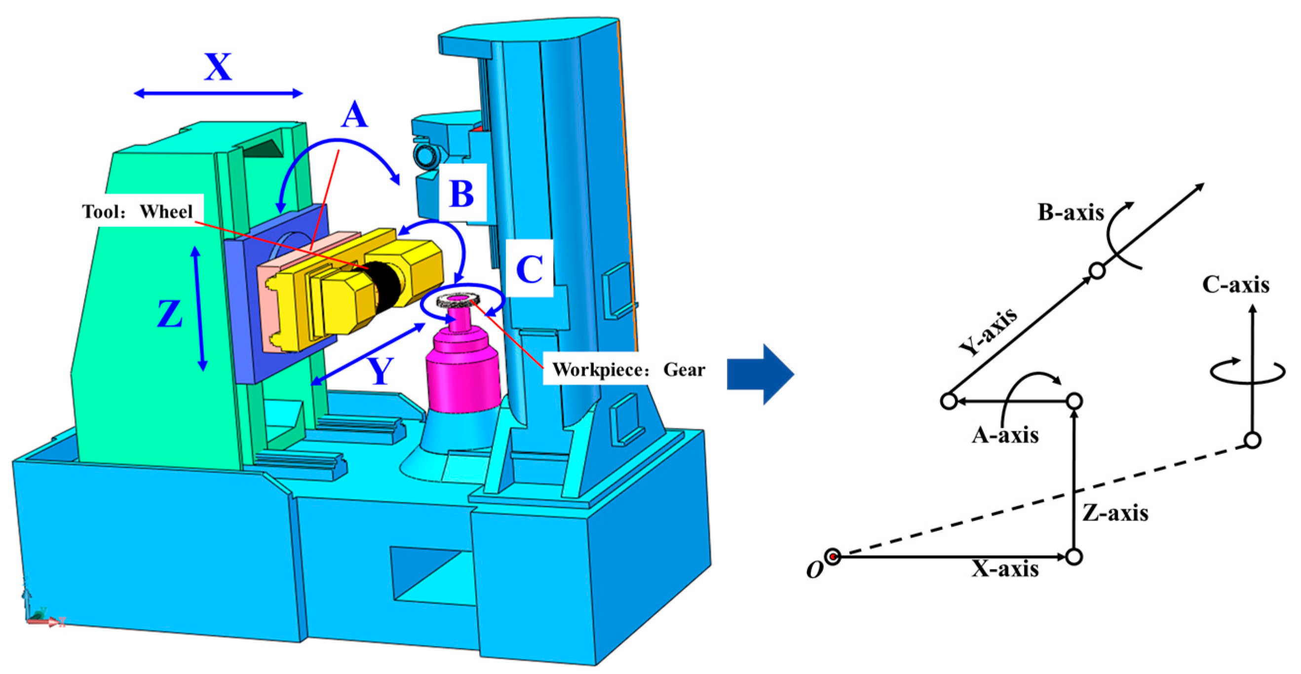
2. Volumetric Error Model of the Gear Grinding Machine

As shown in Figure 1, the gear grinding machine consists of three linear axes, the X-, Y-, and Z-axis, and three rotary axes, the A-, B- and C-axis. The grinding wheel, serving as the cutting tool, is mounted on the B-axis, while the gear blank, acting as the workpiece, is secured on the C-axis via a fixture. The A-axis functions as the swing axis of the tool-holder structure, enabling angular motion of the tool around the X-axis. The machine’s structure can be simplified into two kinematic chains: O–C and O–X–Z–A–Y–B, where O represents the machine bed.

The volumetric error of the gear grinding machine comprises both motion errors and assembly errors from each axis. To establish the geometric error model, the following fundamental assumptions are adopted:

(1) Rigid-body kinematics: All structural components are assumed to maintain perfect rigidity during operation, with no elastic deformation considered.

(2) Independent axis motion: Dynamic coupling effects between linear and rotary axes are neglected in the error modeling process.

(3) Quasi-static condition: The model excludes time-dependent errors from axis acceleration/deceleration and thermal-induced errors from environmental or operational temperature variations.

(4) Precision spindle assumption: The B-axis, functioning as a high-precision spindle with stringent assembly tolerances, is considered to contribute negligible error to the overall volumetric error model.

The errors of the remaining five axes can be categorized into two types: position-dependent geometric errors (PDGEs) and position-independent geometric errors (PIGEs), as listed in

Table 1. Forty-one geometric errors of the grinding machine.

Axis	PDGEs						PIGEs
X	δxx	δyx	δzx	εxx	εyx	εzx
Z	δxz	δyz	δzz	εxz	εyz	εzz			Sxz
A	δxa	δya	δza	εxa	εya	εza	δoyA	δozA	εoyA	εozA
Y	δxy	δyy	δzy	εxy	εyy	εzy			Sxy	Szy
C	δxc	δyc	δzc	εxc	εyc	εzc	δoxC	δoyC	εoxC	εoyC

. The symbol δ represents the translational errors, while the symbol ε represents the angular errors, and the second subscript represents the target axis to which the error belongs, while the first subscript represents the error direction along or around the coordinate axis. In this case, the error δ_yx represents the translational error of X-axis along the Y direction, which is known as the straightness error. The remaining symbols of the PDGEs follow this naming convention.

In contrast to the PDGEs, the PIGEs primarily reflect the assembly inaccuracies and have constant values. In total, 11 PIGEs can be defined depending on the structure of the gear grinding manche; 3 PIGEs exist between the three linear axes, including squareness error S_xz between the Z-axis and X-axis, squareness error S_xy between the Y-axis and X-axis, and squareness error S_zy between the Y-axis and Z-axis. The theoretical axis of the A-axis is perpendicular to the YZ plane, and four PIGEs exist, including two translational errors along the Y and Z direction, δ_oyA and δ_ozA, and two angular errors around the Y and Z direction, ε_oyA and ε_ozA. The theoretical axis of the C-axis is perpendicular to the XY plane, and another four PIGEs exist, including two translational errors along the X direction, δ_oxC and δ_oyC, and two angular errors around the X direction, ε_oxC and ε_oyC. The whole descriptions of the PDGEs and PIGEs are listed in the Abbreviations.

The inertial coordinate system can be defined on the bed, coinciding with the initial motion position of the X-axis. The C-axis is positioned on one side of the bed, perpendicular to the horizontal plane. The angular velocity vector of the C-axis is denoted as ω_C = [0 0 1]^T, and the position vector of the axis line is denoted as r_C, where r_C = [x_c y_c z_c]^T represents the coordinates of any point on the axis line of the C-axis. Then, the twist expression of the C-axis motion can be denoted as ξ_C = [ω_C v_C]^T, where v_C = r_C × ω_C represents the corresponding linear velocity vector of position vector r_C. The motion transformation T_C can be expressed as shown in Equation (1) when the C-axis rotates by θ_C, where the symbol (^) of ${\hat{\mathit{\xi }}}_C$ is defined for the vector-to-matrix conversion.

$${\mathit{T}}_C=e^{{\hat{\mathit{\xi }}}_C\cdot {\theta }_C}$$

(1)

Similarly, the angular velocity vectors and position vectors of other axes can be obtained as well as the corresponding twist expression, as shown in

Table 2. Twist expression of each axis of the grinding machine.

Axis	Angular Velocity Vector	Position Vector	Linear Velocity Vector	Twist Expression
X	0	—	${\mathit{v}}_X={\left[\begin{array}{ccc}1& 0& 0\end{array}\right]}^T$	${\mathit{\xi }}_X={\left[\begin{array}{cc}{0}_{3\times 1}& {\mathit{v}}_X\end{array}\right]}^T$
Y	0	—	${\mathit{v}}_Y={\left[\begin{array}{ccc}0& 1& 0\end{array}\right]}^T$	${\mathit{\xi }}_Y={\left[\begin{array}{cc}{0}_{3\times 1}& {\mathit{v}}_Y\end{array}\right]}^T$
Z	0	—	${\mathit{v}}_Z={\left[\begin{array}{ccc}0& 0& 1\end{array}\right]}^T$	${\mathit{\xi }}_Z={\left[\begin{array}{cc}{0}_{3\times 1}& {\mathit{v}}_Z\end{array}\right]}^T$
A	${\mathit{\omega }}_A={\left[\begin{array}{ccc}1& 0& 0\end{array}\right]}^T$	${\mathit{r}}_A={[\begin{array}{ccc}{x}_a& y_a& z_a\end{array}]}^T$	${\mathit{v}}_A={\mathit{r}}_A\times {\mathit{\omega }}_A$	${\mathit{\xi }}_A={\left[\begin{array}{cc}{\mathit{\omega }}_A& {\mathit{v}}_A\end{array}\right]}^T$
B	${\mathit{\omega }}_B={\left[\begin{array}{ccc}0& 1& 0\end{array}\right]}^T$	${\mathit{r}}_B={[\begin{array}{ccc}{x}_b& y_b& z_b\end{array}]}^T$	${\mathit{v}}_B={\mathit{r}}_B\times {\mathit{\omega }}_B$	${\mathit{\xi }}_B={\left[\begin{array}{cc}{\mathit{\omega }}_B& {\mathit{v}}_B\end{array}\right]}^T$
C	${\mathit{\omega }}_C={\left[\begin{array}{ccc}0& 0& 1\end{array}\right]}^T$	${\mathit{r}}_C={[\begin{array}{ccc}{x}_c& y_c& z_c\end{array}]}^T$	${\mathit{v}}_C={\mathit{r}}_C\times {\mathit{\omega }}_C$	${\mathit{\xi }}_C={\left[\begin{array}{cc}{\mathit{\omega }}_C& {\mathit{v}}_C\end{array}\right]}^T$

.

The initial positions of the tool and workpiece are denoted as T_BT(0) and T_BW(0), respectively. After the motion θ_X, θ_Y, θ_Z, θ_A, θ_B, and θ_C, the motion transformation matrix from the tool and the workpiece to the bed, T_BT and T_BW, can be expressed as shown in Equation (2).

$$\left\{\begin{array}{l}{\mathit{T}}_{BT}={\mathit{T}}_X\cdot {\mathit{T}}_Z\cdot {\mathit{T}}_A\cdot {\mathit{T}}_Y\cdot {\mathit{T}}_B\cdot {\mathit{T}}_{BT}(0)=e^{{\hat{\mathit{\xi }}}_X\cdot {\theta }_X}\cdot e^{{\hat{\mathit{\xi }}}_Z\cdot {\theta }_Z}\cdot e^{{\hat{\mathit{\xi }}}_A\cdot {\theta }_A}\cdot e^{{\hat{\mathit{\xi }}}_Y\cdot {\theta }_Y}\cdot e^{{\hat{\mathit{\xi }}}_B\cdot {\theta }_B}\cdot {\mathit{T}}_{BT}(0)\\ {\mathit{T}}_{BW}={\mathit{T}}_C\cdot {\mathit{T}}_{BW}(0)=e^{{\hat{\mathit{\xi }}}_C\cdot {\theta }_C}\cdot {\mathit{T}}_{BW}(0)\end{array}\right.$$

(2)

The theoretical tool–workpiece motion transformation can be obtained as shown in Equation (4). Since T_BT(0) and T_BW(0) represents initial position of the tool and the workpiece with constant values, the transformation matrix caused by the axis motions T_WTi can be simplified as Equation (4).

$${\mathit{T}}_{WB}\cdot {\mathit{T}}_{BT}={({\mathit{T}}_{BW})}^{-1}\cdot {\mathit{T}}_{BT}={({\mathit{T}}_{BW}(0))}^{-1}\cdot e^{{\hat{\mathit{\xi }}}_C\cdot (-{\theta }_C)}\cdot e^{{\hat{\mathit{\xi }}}_X\cdot {\theta }_X}\cdot e^{{\hat{\mathit{\xi }}}_Z\cdot {\theta }_Z}\cdot e^{{\hat{\mathit{\xi }}}_A\cdot {\theta }_A}\cdot e^{{\hat{\mathit{\xi }}}_Y\cdot {\theta }_Y}\cdot e^{{\hat{\mathit{\xi }}}_B\cdot {\theta }_B}\cdot {\mathit{T}}_{BT}(0)$$

(3)

$${\mathit{T}}_{WTi}=e^{{\hat{\mathit{\xi }}}_C\cdot (-{\theta }_C)}\cdot e^{{\hat{\mathit{\xi }}}_X\cdot {\theta }_X}\cdot e^{{\hat{\mathit{\xi }}}_Z\cdot {\theta }_Z}\cdot e^{{\hat{\mathit{\xi }}}_A\cdot {\theta }_A}\cdot e^{{\hat{\mathit{\xi }}}_Y\cdot {\theta }_Y}\cdot e^{{\hat{\mathit{\xi }}}_B\cdot {\theta }_B}$$

(4)

T_WTi is also named as the kinematic model of a machine tool, which can reflect the theoretical tool–workpiece position and attitude transformation with theoretical axis motion. To describe the actual motion transformation, the 41 geometric errors listed in Table 1 are superimposed in the theoretical kinematic model. Taking the Y-axis as an example, six PDGEs and two PIGEs are listed in

Table 3. Geometric errors of Y-axis.

Axis	PDGE						PIGEs
Y-axis	δxy	δyy	δzy	εxy	εyy	εzy	Sxy	Szy

, and the motion transformation matrix of these eight geometric errors can be expressed as Equation (5). Similarly, the comprehensive error motion transformation of the X-, Z-, A-, and C-axis can be obtained as shown in Equation (6).

$$\mathit{E}{\mathit{T}}_Y=e^{{\hat{\mathit{\xi }}}_{\mathit{X}}\cdot {\delta }_{xy}}\cdot e^{{\hat{\mathit{\xi }}}_Y\cdot {\delta }_{yy}}\cdot e^{{\hat{\mathit{\xi }}}_Z\cdot {\delta }_{zy}}\cdot e^{{\hat{\mathit{\xi }}}_A\cdot ({\epsilon }_{xy}+S_{zy})}\cdot e^{{\hat{\mathit{\xi }}}_B\cdot {\epsilon }_{yy}}\cdot e^{{\hat{\mathit{\xi }}}_C\cdot ({\epsilon }_{zy}+S_{xy})}$$

(5)

$$\left\{\begin{array}{l}\mathit{E}{\mathit{T}}_X=e^{{\hat{\mathit{\xi }}}_X\cdot {\delta }_{xx}}\cdot e^{{\hat{\mathit{\xi }}}_Y\cdot {\delta }_{yx}}\cdot e^{{\hat{\mathit{\xi }}}_Z\cdot {\delta }_{zx}}\cdot e^{{\hat{\mathit{\xi }}}_A\cdot {\epsilon }_{xx}}\cdot e^{{\hat{\mathit{\xi }}}_B\cdot {\epsilon }_{yx}}\cdot e^{{\hat{\mathit{\xi }}}_C\cdot {\epsilon }_{zx}}\\ \mathit{E}{\mathit{T}}_Z=e^{{\hat{\mathit{\xi }}}_X\cdot {\delta }_{xz}}\cdot e^{{\hat{\mathit{\xi }}}_Y\cdot {\delta }_{yz}}\cdot e^{{\hat{\mathit{\xi }}}_Z\cdot {\delta }_{zz}}\cdot e^{{\hat{\mathit{\xi }}}_A\cdot {\epsilon }_{xz}}\cdot e^{{\hat{\mathit{\xi }}}_B\cdot ({\epsilon }_{yz}+S_{zx})}\cdot e^{{\hat{\mathit{\xi }}}_C\cdot {\epsilon }_{zz}}\\ \mathit{E}{\mathit{T}}_A=e^{{\hat{\mathit{\xi }}}_X\cdot {\delta }_{xa}}\cdot e^{{\hat{\mathit{\xi }}}_Y\cdot ({\delta }_{ya}+{\delta }_{oyA})}\cdot e^{{\hat{\mathit{\xi }}}_Z\cdot ({\delta }_{za}+{\delta }_{ozA})}\cdot e^{{\hat{\mathit{\xi }}}_A\cdot {\epsilon }_{xa}}\cdot e^{{\hat{\mathit{\xi }}}_B\cdot ({\epsilon }_{ya}+{\epsilon }_{oyA})}\cdot e^{{\hat{\mathit{\xi }}}_C\cdot ({\epsilon }_{za}+{\epsilon }_{ozA})}\\ \mathit{E}{\mathit{T}}_C=e^{{\hat{\mathit{\xi }}}_X\cdot ({\delta }_{xc}+{\delta }_{oxC})}\cdot e^{{\hat{\mathit{\xi }}}_Y\cdot ({\delta }_{yc}+{\delta }_{oyC})}\cdot e^{{\hat{\mathit{\xi }}}_Z\cdot {\delta }_{zc}}\cdot e^{{\hat{\mathit{\xi }}}_A\cdot ({\epsilon }_{xc}+{\epsilon }_{oxC})}\cdot e^{{\hat{\mathit{\xi }}}_B\cdot ({\epsilon }_{yc}+{\epsilon }_{oyC})}\cdot e^{{\hat{\mathit{\xi }}}_C\cdot {\epsilon }_{zc}}\end{array}\right.$$

(6)

Therefore, when all the error motions are considered, the motion transformation matrix from the tool to the workpiece can be obtained as shown in Equation (7), also known as the volumetric error model.

$${\mathit{T}}_{WT}={(\mathit{E}{\mathit{T}}_C\cdot {\mathit{T}}_C)}^{-1}\cdot \mathit{E}{\mathit{T}}_X\cdot {\mathit{T}}_X\cdot \mathit{E}{\mathit{T}}_Z\cdot {\mathit{T}}_Z\cdot \mathit{E}{\mathit{T}}_A\cdot {\mathit{T}}_A\cdot \mathit{E}{\mathit{T}}_Y\cdot {\mathit{T}}_Y\cdot \mathit{E}{\mathit{T}}_B\cdot {\mathit{T}}_B$$

(7)

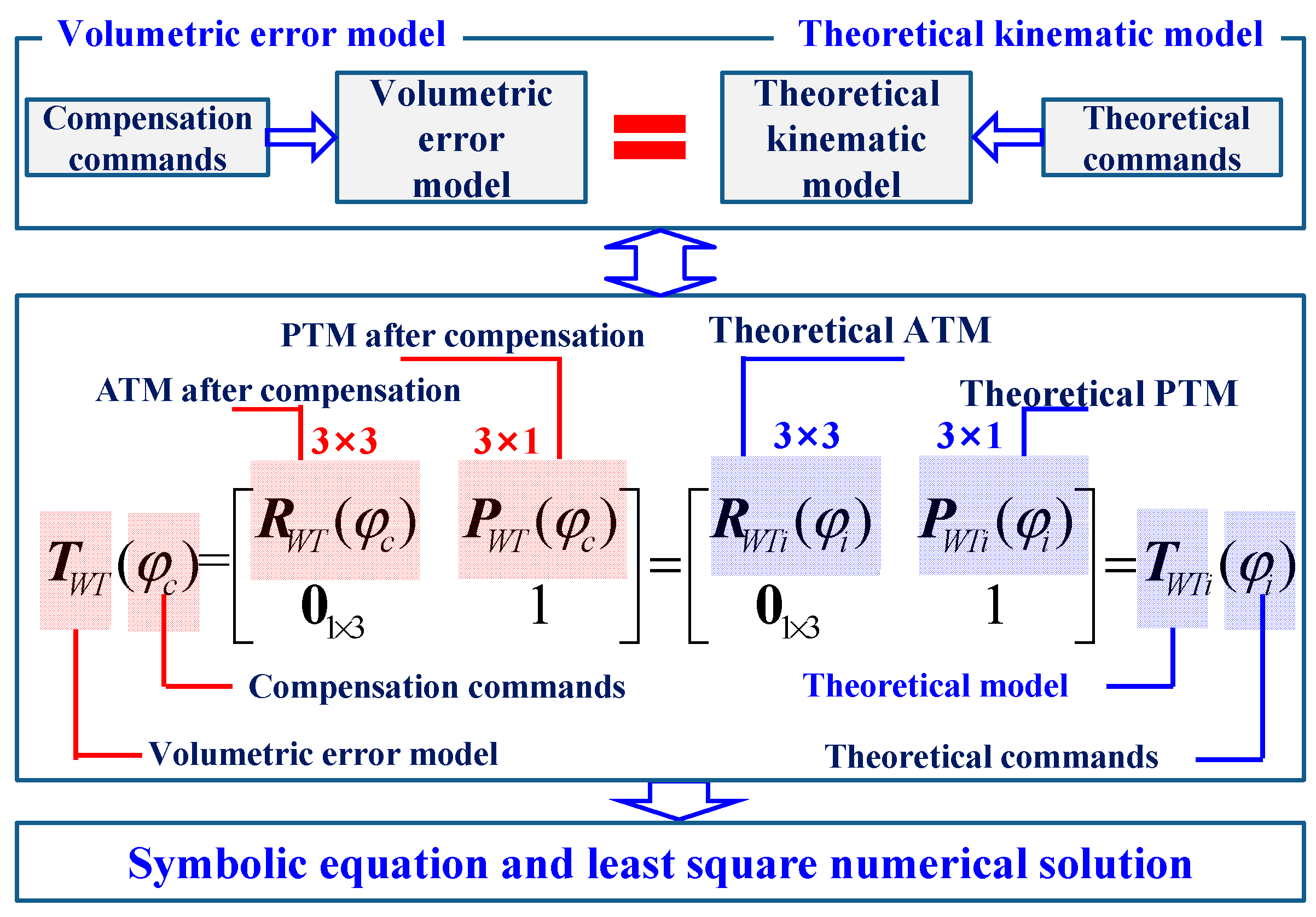
3. Decoupling Solution of the Volumetric Error Model

3.1. Numerical Solution

With theoretical axis motion, the kinematics model ${\mathit{T}}_{WTi}$ is composed of the attitude transformation matrix (ATM), denoted as ${\mathit{R}}_{WTi}$, and the position transformation matrix (PTM), denoted as ${\mathit{P}}_{WTi}$, as shown in Equation (8) [30,31], and the theoretical axis motion command can be expressed as a vector ${\phi }_i=\left\{a_i,b_i,c_i,x_i,y_i,z_i\right\}$.

$${\mathit{T}}_{WTi}=\left[\begin{array}{cc}{\mathit{R}}_{WTi}& {\mathit{P}}_{WTi}\\ 0_{1\times 3}& 1\end{array}\right]$$

(8)

Similarly, the volumetric error model ${\mathit{T}}_{WT}$, describing the actual motion transformation, can be expressed as Equation (9), where ${\mathit{R}}_{WT}$ and ${\mathit{P}}_{WT}$ represent ATM and PTM, respectively, when considering the geometric errors.

$${\mathit{T}}_{WT}=\left[\begin{array}{cc}{\mathit{R}}_{WT}& {\mathit{P}}_{WT}\\ 0_{1\times 3}& 1\end{array}\right]$$

(9)

To eliminate or reduce the influence of geometric errors, the volumetric error model ${\mathit{T}}_{WT}$ needs to be decoupled to obtain the compensation motion commands of axes, and the original theoretical axis motion commands are replaced, as shown in Equation (10), where ${\phi }_c=\left\{a_c,b_c,c_c,x_c,y_c,z_c\right\}$ is the compensation motion commands.

$${\mathit{T}}_{WT}({\mathit{\phi }}_c)=\left[\begin{array}{cc}{\mathit{R}}_{WT}\left({\mathit{\phi }}_c\right)& {\mathit{P}}_{WT}\left({\mathit{\phi }}_c\right)\\ 0_{1\times 3}& 1\end{array}\right]=\left[\begin{array}{cc}{\mathit{R}}_{WTi}\left({\mathit{\phi }}_i\right)& {\mathit{P}}_{WTi}\left({\mathit{\phi }}_i\right)\\ 0_{1\times 3}& 1\end{array}\right]={\mathit{T}}_{WTi}({\mathit{\phi }}_i)$$

(10)

The numerical solution is a universal method aside from its lack of analytical properties, and the process is shown in Figure 2. Specifically, ${\mathit{R}}_{WT}\left({\mathit{\phi }}_c\right)$ is set equal to ${\mathit{R}}_{WTi}\left({\mathit{\phi }}_i\right)$, ${\mathit{P}}_{WT}\left({\mathit{\phi }}_c\right)$ is set equal to ${\mathit{P}}_{WTi}\left({\mathit{\phi }}_i\right)$, and a total of 12 symbolic equations are established and solved directly through numerical methods. The numerical solution is feasible when offline and with sufficient computing resources, although it cannot be used as a real-time compensation method. In this work, the numerical solution is used as a comparative reference for the subsequent proposed method.

In this part, three sets of axis motion commands are used as a simulation case to study the inverse numerical solution of the volumetric error model, namely, ${\mathit{\phi }}_1$, ${\mathit{\phi }}_2$, and ${\mathit{\phi }}_3$, as shown in Equation (11). In these positions of the axes, the 41 errors are set to random value 10 times for each group under each set of axis motion, where the translational error ranges from −20 μm to 20 μm, while the angular error ranges from −80 μrad to 80 μrad. The root mean square errors (RMSEs) of ATM and PTM are calculated as shown in Equation (12), and the comparison of results after decoupling and compensation is shown in Figure 3, where ‘Comp.’ is an abbreviation for the word ‘compensation’. In the simulation of cumulative 30 groups of random errors, the RMSE after compensation shows a significant improvement over the original state.

$$\left\{\begin{array}{l}{\mathit{\phi }}_1=\left\{\begin{array}{llllll}{a}_1=20°\hfill & b_1=40°\hfill & c_1=60°\hfill & x_1=350\mathrm{mm}\hfill & y_1=80\mathrm{mm}\hfill & z_1=250\mathrm{mm}\hfill \end{array}\right\}\\ {\mathit{\phi }}_2=\left\{\begin{array}{llllll}{a}_2=30°\hfill & b_2=50°\hfill & c_2=70°\hfill & x_2=400\mathrm{mm}\hfill & y_2=40\mathrm{mm}\hfill & z_2=350\mathrm{mm}\hfill \end{array}\right\}\\ {\mathit{\phi }}_3=\left\{\begin{array}{llllll}{a}_3=-30°\hfill & b_3=200°\hfill & c_3=300°\hfill & x_3=450\mathrm{mm}\hfill & y_3=120\mathrm{mm}\hfill & z_3=400\mathrm{mm}\hfill \end{array}\right\}\end{array}\right.$$

(11)

$$\left\{\begin{array}{c}RMS{E}_R=\left\{\begin{array}{c}\sqrt{{\displaystyle \frac{1}{9}}{\displaystyle \sum _{j=1}^9{\left({\mathit{R}}_{WTi}^j({\mathit{\phi }}_i)-{\mathit{R}}_{WT}^j({\mathit{\phi }}_i)\right)}^2}},\hspace{1em}\mathrm{Before}\hspace{1em}\mathrm{Compensation}\\ \sqrt{{\displaystyle \frac{1}{9}}{\displaystyle \sum _{j=1}^9{\left({\mathit{R}}_{WTi}^j({\mathit{\phi }}_i)-{\mathit{R}}_{WT}^j({\mathit{\phi }}_c)\right)}^2}},\hspace{1em}\mathrm{After}\hspace{1em}\mathrm{Compensation}\end{array}\right.\\ RMS{E}_P=\left\{\begin{array}{c}\sqrt{{\displaystyle \frac{1}{3}}{\displaystyle \sum _{j=1}^3{\left({\mathit{P}}_{WTi}^j({\mathit{\phi }}_i)-{\mathit{P}}_{WT}^j({\mathit{\phi }}_i)\right)}^2}},\hspace{1em}\mathrm{Before}\hspace{1em}\mathrm{Compensation}\\ \sqrt{{\displaystyle \frac{1}{3}}{\displaystyle \sum _{j=1}^3{\left({\mathit{P}}_{WTi}^j({\mathit{\phi }}_i)-{\mathit{P}}_{WT}^j({\mathit{\phi }}_c)\right)}^2}},\hspace{1em}\mathrm{After}\hspace{1em}\mathrm{Compensation}\end{array}\right.\end{array}\right.$$

(12)

3.2. Analytical Decoupling Based on POE

The Jacobian matrix is commonly used to map the joint velocity and actuator velocity in robot mechanisms. Based on POE, the tool–workpiece Jacobian matrix can be clearly derived. The motion transformation T_WT(φ) consists of the ATM, R(φ), and the PTM, P(φ), as shown in Equation (13), where φ represents the axis motion commands. For convenience, the C(-)-, X-, Z-, A-, Y-, and B-axis were numbered as 1, 2, 3, 4, 5, and 6, where C(-) indicates the reverse motion of the C-axis.

$${\mathit{T}}_{WT}(\mathit{\phi })=\left[\begin{array}{cc}\mathit{R}(\mathit{\phi })& \mathit{P}(\mathit{\phi })\\ 0_{1\times 3}& 1\end{array}\right]$$

(13)

Then, the tool–workpiece instantaneous volumetric velocity $\hat{\mathit{V}}$ can be expressed as shown in Equation (14).

$$\hat{\mathit{V}}={\dot{\mathit{T}}}_{WT}(\mathit{\phi })\cdot {\mathit{T}}_{WT}^{-1}(\mathit{\phi })={\displaystyle \sum _{i=1}^n\left(\frac{\partial {\mathit{T}}_{WT}}{\partial {\phi }_i}{\dot{\phi }}_i\right){\mathit{T}}_{WT}^{-1}(\mathit{\phi })}={\displaystyle \sum _{i=1}^n\left(\frac{\partial {\mathit{T}}_{WT}}{\partial {\phi }_i}{\mathit{T}}_{WT}^{-1}(\mathit{\phi })\right)}\cdot {\dot{\phi }}_i$$

(14)

Combining with Equation (13), $\hat{\mathit{V}}$ can be expressed as Equation (15).

$$\hat{\mathit{V}}={\dot{\mathit{T}}}_{WT}(\mathit{\phi })\cdot {\mathit{T}}_{WT}^{-1}(\mathit{\phi })=\left[\begin{array}{cc}\dot{\mathit{R}}{\mathit{R}}^T& -\dot{\mathit{R}}{\mathit{R}}^T\mathit{P}+\dot{\mathit{P}}\\ 0_{1\times 3}& 1\end{array}\right]$$

(15)

The corresponding twist expression of $\hat{\mathit{V}}$ can be expressed as Equation (16).

$$\mathit{V}=\left(\begin{array}{c}\mathit{\omega }\\ \mathit{v}\end{array}\right)=\left(\begin{array}{c}{(\dot{\mathit{R}}{\mathit{R}}^T)}^{\vee }\\ -\dot{\mathit{R}}{\mathit{R}}^T\mathit{P}+\dot{\mathit{P}}\end{array}\right)={{\displaystyle \sum _{i=1}^n\left(\frac{\partial {\mathit{T}}_{WT}}{\partial {\phi }_i}{\mathit{T}}_{WT}^{-1}(\mathit{\phi })\right)}}^{\vee }\cdot {\dot{\phi }}_i$$

(16)

Then, the linear relationship can be obtained between the volumetric velocity V and the velocity of each axis $\dot{\mathit{\phi }}$, as shown in Equations (17) and (18).

$$\left\{\begin{array}{l}\mathit{J}(\mathit{\phi })=\left(\begin{array}{l}{\left({\displaystyle \frac{\partial \mathit{T}}{\partial {\phi }_1}}{\mathit{T}}^{-1}(\mathit{\phi })\right)}^{\vee },{\left({\displaystyle \frac{\partial \mathit{T}}{\partial {\phi }_2}}{\mathit{T}}^{-1}(\mathit{\phi })\right)}^{\vee },\\ \dots ,{\left({\displaystyle \frac{\partial \mathit{T}}{\partial {\phi }_n}}{\mathit{T}}^{-1}(\mathit{\phi })\right)}^{\vee }\end{array}\right)\\ {\dot{\mathit{\phi }}}_i=({\dot{\phi }}_1,\dots ,{\dot{\phi }}_n{)}^{\mathit{T}}\end{array}\right.$$

(17)

$$\mathit{V}=\mathit{J}(\phi )\cdot \dot{\mathit{\phi }}=\left({\mathit{\xi }}_1^{*},{\mathit{\xi }}_2^{*},{\mathit{\xi }}_3^{*},\dots ,{\mathit{\xi }}_n^{*}\right)\left(\begin{array}{c}{\dot{\phi }}_1\\ {\dot{\phi }}_2\\ ⋮\\ {\dot{\phi }}_n\end{array}\right)$$

(18)

Specially, for the rotary axis, ${\xi }_i^{*}$ can be calculated as Equation (19), where ${\omega }_i^{*}$ represents the unit vector of axis line, which can be calculated as Equation (20), and $r_i^{*}$ represents the position vector of any point on the axis line, which can be calculated as Equation (21).

$${\mathit{\xi }}_i^{*}=\left(\begin{array}{c}{\mathit{\omega }}_{\mathit{i}}^{*}\\ {\mathit{r}}_{\mathit{i}}^{*}\times {\mathit{\omega }}_{\mathit{i}}^{*}\end{array}\right)$$

(19)

$${\mathit{\omega }}_{\mathit{i}}^{*}=e^{{\hat{\mathit{\omega }}}_1\cdot {\phi }_1}\cdot e^{{\hat{\mathit{\omega }}}_2\cdot {\phi }_2}\dots \cdot e^{{\hat{\mathit{\omega }}}_{i-1}\cdot {\phi }_{i-1}}\cdot {\mathit{\omega }}_i$$

(20)

$$\left(\begin{array}{c}{\mathit{r}}_{\mathit{i}}^{*}\\ 1\end{array}\right)=e^{{\hat{\mathit{\xi }}}_1\cdot {\phi }_1}\cdot e^{{\hat{\mathit{\xi }}}_2\cdot {\phi }_2}\dots e^{{\hat{\mathit{\xi }}}_{i-1}\cdot {\phi }_{i-1}}\left(\begin{array}{c}{\mathit{r}}_i\\ 1\end{array}\right)$$

(21)

For linear axis, ${\xi }_i^{*}$ can be calculated as Equation (21).

$${\mathit{\xi }}_i^{*}=\left(\begin{array}{c}{0}_{3\times 1}\\ {\mathit{v}}_{\mathit{i}}^{*}\end{array}\right)=\left(\begin{array}{c}{0}_{3\times 1}\\ e^{{\hat{\mathit{\omega }}}_1\cdot {\phi }_1}\cdot e^{{\hat{\mathit{\omega }}}_2\cdot {\phi }_2}\dots \cdot e^{{\hat{\mathit{\omega }}}_{i-1}\cdot {\phi }_{i-1}}\cdot {\mathit{r}}_i\end{array}\right)$$

(22)

According to the forward kinematics model of the gear grinding machine, the volumetric velocity V and the Jacobian matrix J can be obtained as expressed in Equation (21).

$$\mathit{V}=\left(\begin{array}{c}\mathit{\omega }\\ \mathit{v}\end{array}\right)=\mathit{J}\cdot \dot{\mathit{\phi }}=\left[\begin{array}{cccccc}{\mathit{\xi }}_C^{*}& {\mathit{\xi }}_X^{*}& {\mathit{\xi }}_Z^{*}& {\mathit{\xi }}_A^{*}& {\mathit{\xi }}_Y^{*}& {\mathit{\xi }}_B^{*}\end{array}\right]\cdot {\left[\begin{array}{cccccc}\dot{c}& \dot{x}& \dot{z}& \dot{a}& \dot{y}& \dot{b}\end{array}\right]}^T$$

(23)

On the other hand, the volumetric velocity can be derived from the volumetric pose by combining Equation (16), and Equation (23) be expressed as Equation (24).

$$\mathit{V}=\left(\begin{array}{c}{({\displaystyle \frac{d\mathit{R}}{dt}}{\mathit{R}}^T)}^{\vee }\\ -{\displaystyle \frac{d\mathit{R}}{dt}}{\mathit{R}}^T\mathit{P}+{\displaystyle \frac{d\mathit{P}}{dt}}\end{array}\right)=\mathit{J}\cdot \dot{\mathit{\phi }}={\displaystyle \frac{\mathit{J}\cdot {\left[\begin{array}{cccccc}dc& dx& dz& da& dy& db\end{array}\right]}^T}{dt}}$$

(24)

Since the displacement and rotation of the axis motion caused by the error as well as the change of tool–workpiece volumetric pose are very small, Equation (24) can be further simplified as Equation (25), where ΔR and ΔP, respectively, represent changes of the tool–workpiece attitude and position, that is, attitude matrix error and position vector error, while Δc, Δx, Δz, Δa, Δy, and Δb represent the change of each axis motion of the gear grinding machine, which can also indicate the compensation motion command of each axis.

$$\left(\begin{array}{c}{(\Delta \mathit{R}{\mathit{R}}^T)}^{\vee }\\ -\Delta \mathit{R}{\mathit{R}}^T\mathit{P}+\Delta \mathit{P}\end{array}\right)=\mathit{J}\cdot {\left[\begin{array}{cccccc}\Delta c& \Delta x& \Delta z& \Delta a& \Delta y& \Delta b\end{array}\right]}^T$$

(25)

Finally, the compensation motion command of each axis can be calculated as Equation (26).

$${\left[\begin{array}{cccccc}\Delta c& \Delta x& \Delta z& \Delta a& \Delta y& \Delta b\end{array}\right]}^T={\mathit{J}}^{-1}\cdot \left(\begin{array}{c}{(\Delta \mathit{R}{\mathit{R}}^T)}^{\vee }\\ -\Delta \mathit{R}{\mathit{R}}^T\mathit{P}+\Delta \mathit{P}\end{array}\right)$$

(26)

The Jacobi matrix based on the POE converts the nonlinear relationship between the tool–workpiece pose and the axis motion to the linear relationship between the tool–workpiece pose change and the axis motion change. Then, the compensation motion command of the axis motion can be obtained with the linear relationship.

Taking the axis motion φ₁, φ₂, and φ₃ and the corresponding geometric errors in Figure 3 as the example, Equation (26) is used for direct decoupling. To distinguish the effect of direct numerical decoupling method (NUMD) and exponential product Jacobian matrix decoupling method (POED), the RMSE between theoretical pose matrix and actual pose matrix before compensation is omitted in Figure 4. The simulation results show that compared with the direct numerical decoupling method NUMD, the POED method can achieve a better decoupling accuracy and compensation effect. More importantly, the POED method can obtain the explicit and analytical expressions of the value compensation motion commands of the axes.

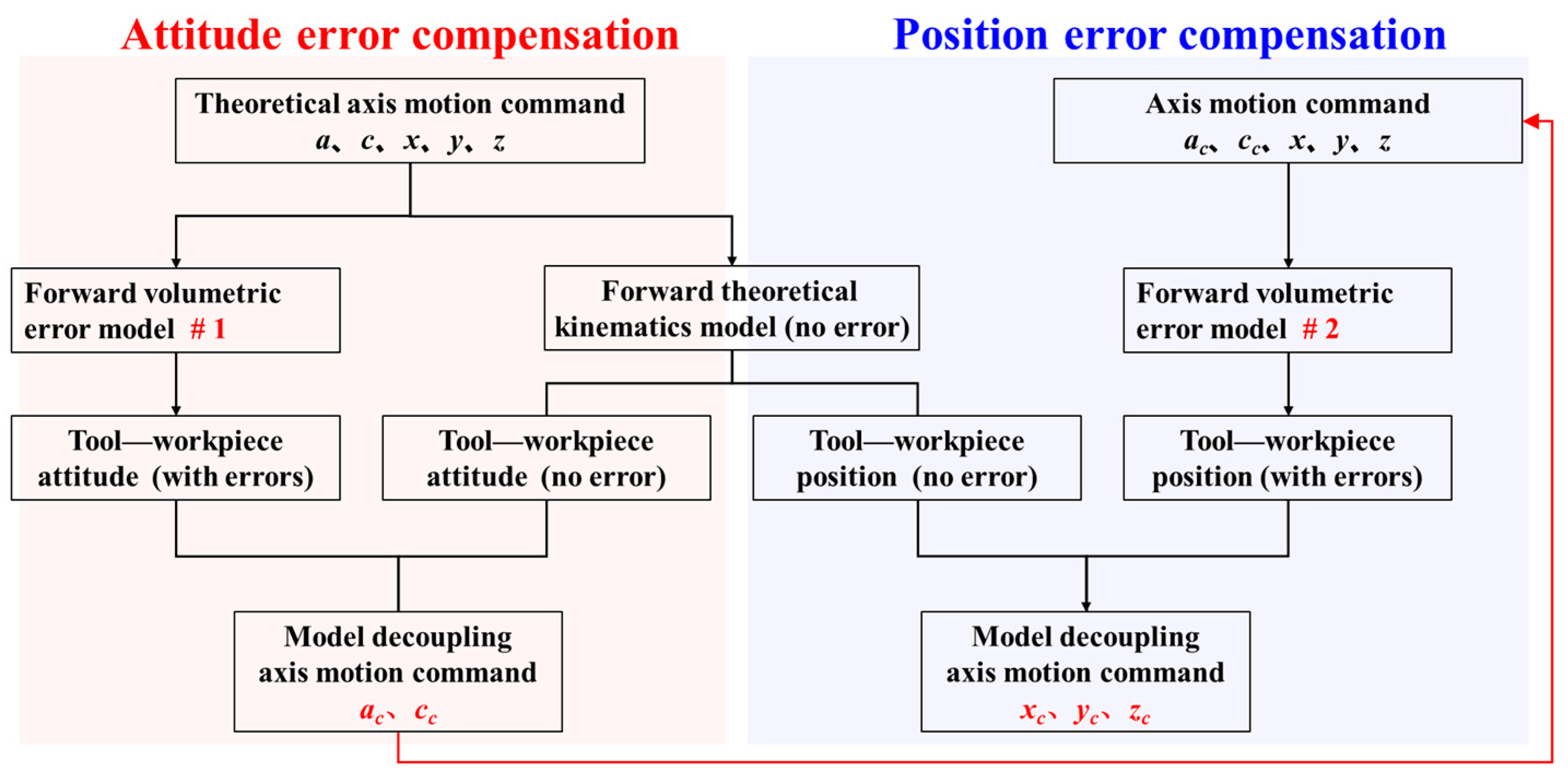
3.3. Step-by-Step Jacobi Decoupling Method Under Compensated Motion Constraints

In the above section, the volumetric error model of the gear grinding machine is inversely solved by the POED method, and the comprehensive error can be compensated with six motion axes, the X-, Y-, Z-, A-, B-, and C-axis. However, when the B-axis is only used as the spindle without high-precision indexing function, only five motion axes participate in forming the tool–workpiece pose, which also means that pose compensation is limited. Then, the Jacobian matrix in Section 3.2 needs to be modified to apply to such cases, as shown in Equation (27).

$$\mathit{J}=\left[\begin{array}{ccccc}{\mathit{\xi }}_C^{*}& {\mathit{\xi }}_X^{*}& {\mathit{\xi }}_Z^{*}& {\mathit{\xi }}_A^{*}& {\mathit{\xi }}_Y^{*}\end{array}\right]$$

(27)

In this way, the Jacobian matrix is no longer a 6 × 6 square array. Correspondingly, the final compensation motion commands of each axis can be modified and expressed as Equation (28), and this decoupling method is denoted as POED-5.

$${\left[\begin{array}{ccccc}\Delta c& \Delta x& \Delta z& \Delta a& \Delta y\end{array}\right]}^T={\left[{\mathit{J}}^T\cdot \mathit{J}\right]}^{-1}\cdot {\mathit{J}}^T\cdot \left(\begin{array}{c}{(\Delta \mathit{R}{\mathit{R}}^T)}^{\vee }\\ -\Delta \mathit{R}{\mathit{R}}^T\mathit{P}+\Delta \mathit{P}\end{array}\right)$$

(28)

A set of simulations is conducted to compare the compensation performance of POED and POED-5, as shown in Figure 5. Compared with the six-axis compensation POED method, the compensation performance of POED-5 is obviously weaker. In detail, the maximum value of the ATM is only reduced from 1.1 × 10⁻⁴ to 3.1 × 10⁻⁵ after compensation, while the maximum value of the PTM is only reduced from 7.0 × 10⁻⁵ to 2.0 × 10⁻⁵.

Considering that the motion of linear axis hardly changes the tool–workpiece attitude in the volumetric error model, a step-by-step decoupling method, denoted as SPOED-5, is proposed in which the attitude error is compensated by the A-axis and C-axis, and then the position error is compensated by the X-, Y-, and Z-axis, as shown in Figure 6.

In the SPOED-5 method, the volumetric error model #1 is first decoupled to obtain the compensation motion commands, a_c and c_c of the A- and C-axis. Next, the compensation motion commands are replaced back to re-establish the volumetric error model #2. Then, the compensation motion commands of three axes, x_c, y_c, and z_c, are then obtained as the inverse solution after decoupling the volumetric error model #2. For the inverse solution of the attitude matrix and the inverse solution of the position matrix, the Jacobian matrix and can be, respectively, expressed as Equation (28).

$$\left\{\begin{array}{l}{\mathit{J}}_R=\left[\begin{array}{cc}{\mathit{\xi }}_C^{*}& {\mathit{\xi }}_A^{*}\end{array}\right]\\ {\mathit{J}}_P=\left[\begin{array}{ccc}{\mathit{\xi }}_X^{*}& {\mathit{\xi }}_Z^{*}& {\mathit{\xi }}_Y^{*}\end{array}\right]\end{array}\right.$$

(29)

Correspondingly, Equation (28) is converted as Equation (30), and $\Delta {\mathit{P}}^{*}$ represents the position matrix error in the volumetric error model #2, where the rotary axis compensation motion commands a_c and c_c are used instead of the original rotary axis motion commands a and c.

$$\left\{\begin{array}{l}{\left[\begin{array}{cc}\Delta c& \Delta a\end{array}\right]}^T={\left[{({\mathit{J}}_R)}^T\cdot {\mathit{J}}_R\right]}^{-1}\cdot {({\mathit{J}}_R)}^T\cdot \Delta \mathit{R}\\ {\left[\begin{array}{ccc}\Delta x& \Delta z& \Delta y\end{array}\right]}^T={\left[{({\mathit{J}}_P)}^T\cdot {\mathit{J}}_P\right]}^{-1}\cdot {({\mathit{J}}_P)}^T\cdot \Delta {\mathit{P}}^{*}\end{array}\right.$$

(30)

To verify the compensation performance of the proposed SPOED-5, a variety of methods are used to inversely solve and compensate the volumetric error, including the NUMD method with six-axis motion, the POED method with six-axis motion, the NUMD-5 with five-axis motion, and the POED-5 method with five-axis motion. The principle of this step-by step decoupling compensation is also applicable to the numerical decoupling method NUMD in Section 3.1, denoted as SNUMD-5. The comparison results are shown in

Table 4. Compensation effect with different methods.

Item		Before Comp. ×10−5	6-Axis Comp.		5-Axis Comp.		5-Axis Step-Comp.
			NUMD ×10−7	POED ×10−9	NUMD-5 ×10−5	POED-5 ×10−5	SNUMD-5 ×10−5	SPOED-5 ×10−5
ATM	ΔR11	−8.4	5.7	−3.8	1.3	1.2	1.3	1.2
	ΔR12	−11.0	19	1.6	−2.0	−2.1	−2.0	−2.1
	ΔR13	2.1	−12	−5.0	3.1	3.1	3.1	3.1
	ΔR21	6.8	−3.2	2.2	−0.76	−0.69	−0.76	−0.69
	ΔR22	−8.7	−11	−1.4	1.2	1.2	1.2	1.2
	ΔR23	−4.3	22	−3.4	0.22	−4.0 × 10−4	0.22	−4.0 × 10−4
	ΔR31	−7.6	−6.9	3.9	−1.6	−1.5	−1.6	−1.5
	ΔR32	2.9	−22	−2.2	2.4	2.5	2.4	2.5
	ΔR33	3.8	−20	−2.6	2.5	2.6	2.5	2.6
PTM	ΔP1	7.0	−5.3	−4.8	−0.05	−1.2	0.03	−4.7 × 10−4
	ΔP2	2.7	56	−6.2	0.56	2.0	0.43	2.6 × 10−4
	ΔP3	2.0	23	7.7	0.23	−0.55	0.2	3.0 × 10−5

.

Some intuitive phenomena can be summarized as follows, and the symbols (>), (<), and (≈) are used to indicate the comparison of compensation performance of different methods.

(1) In general, the compensation performance with six-axis motion is superior to that of with five-axis motion, that is (NUMD, POED) > (NUMD-5, POED-5, SNUMD-5, SPOED-5). This conforms to the basic kinematic principle, where the axis motion on the 5 degrees of freedom cannot completely compensate the pose error on 6 degrees of freedom.

(2) For the ATM, the compensation performances of POED-5 and NUMD-5 is very close, that is, POED-5 ≈ NUMD-5. For the PTM, the compensation performance of POED-5 is better than that of NUMD-5, that is, POED-5 > NUMD-5.

(3) Step-by-step process does not significantly improve the compensation performances of NUMD, while it greatly improves the compensation performance of POED-5, that is, SNUMD-5 ≈ NUMD-5 and SPOED-5 > POED-5.

(4) Specially, for the PTM, the compensation performance of step-by-step SPOED-5 method is better than that of POED with six-axis motion, that is, SPOED-5 > POED.

(5) When the compensation performances of ATM and PTM are considered at the same time, they can be summarized as follows: POED > NUMD > SPOED-5 > SNUMD-5 > POED-5 ≈ NUMD-5.

It should be noted that the compensation object is the tool–workpiece pose transformation matrix of the volumetric error model in Section 2, which does not contain the detailed point coordinates; thus, it cannot express the absolute spatial pose after the pose transformation in the inertial coordinate system. The six-axis compensation method (POED and NUMD) is a full-degree of the freedom error compensation method, which can realize simultaneous compensation of attitude and position. Through the six-axis motion, the compensated actual pose transformation matrix is almost equal to the theoretical pose transformation matrix. In this case, the coordinates of the specific points or rigid bodies can be ignored. However, when using five-axis motion compensation, only the motions of the A- and C-axis are used to compensate the tool–workpiece attitude, which cannot completely compensate the attitude error. In this way, the uncompensated attitude error will further affect the tool–workpiece position error. Therefore, when using SPOED-5 to compensate for the pose error, it is necessary to combine the targeted point coordinates, and this part is compared and explained with a detailed example in the following Section 5.2.

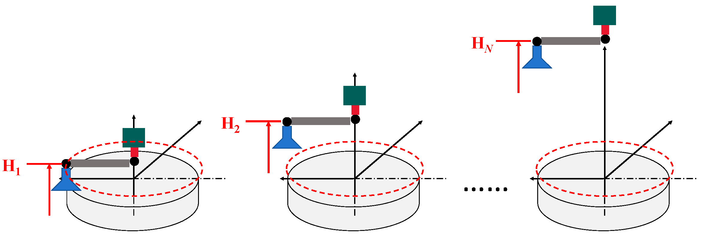
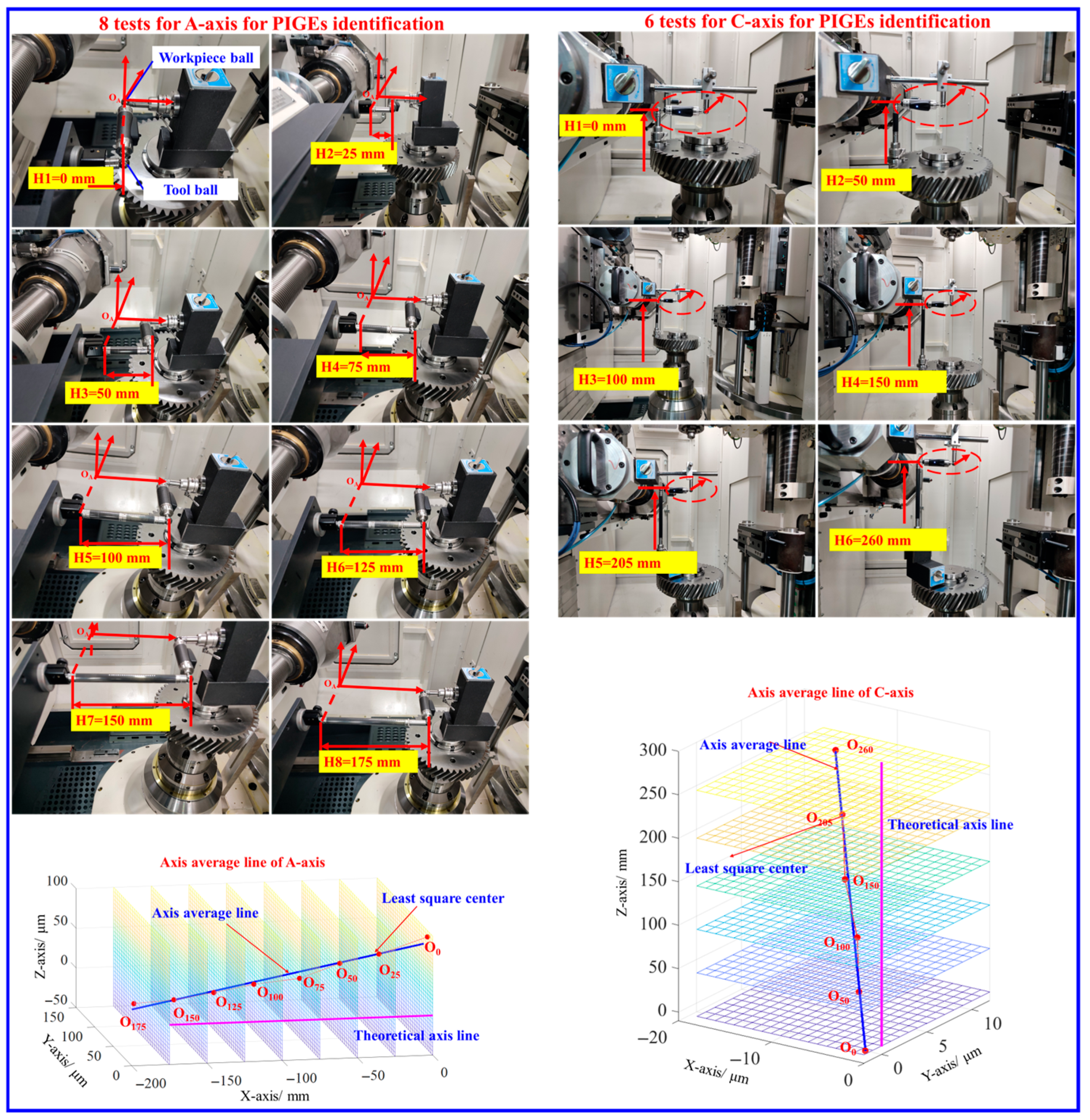
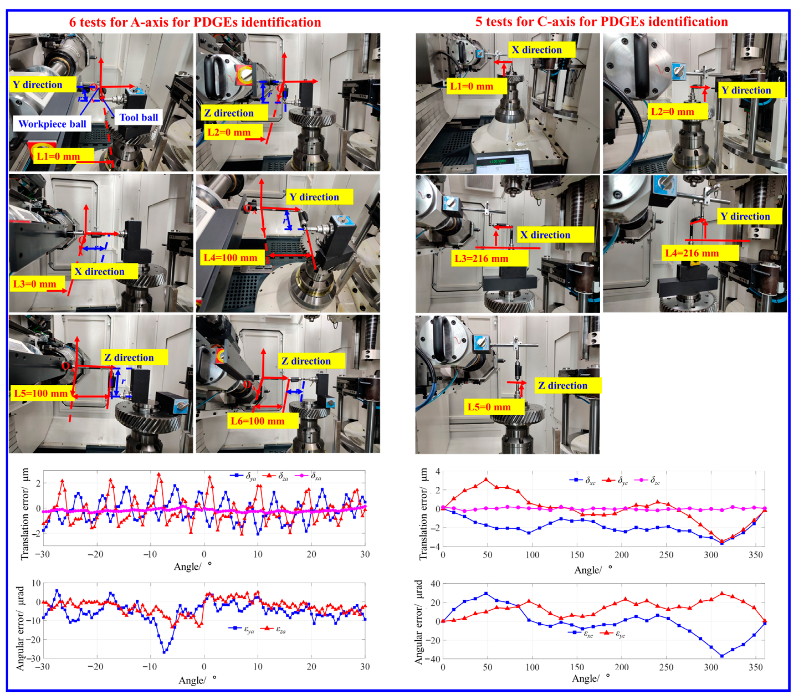
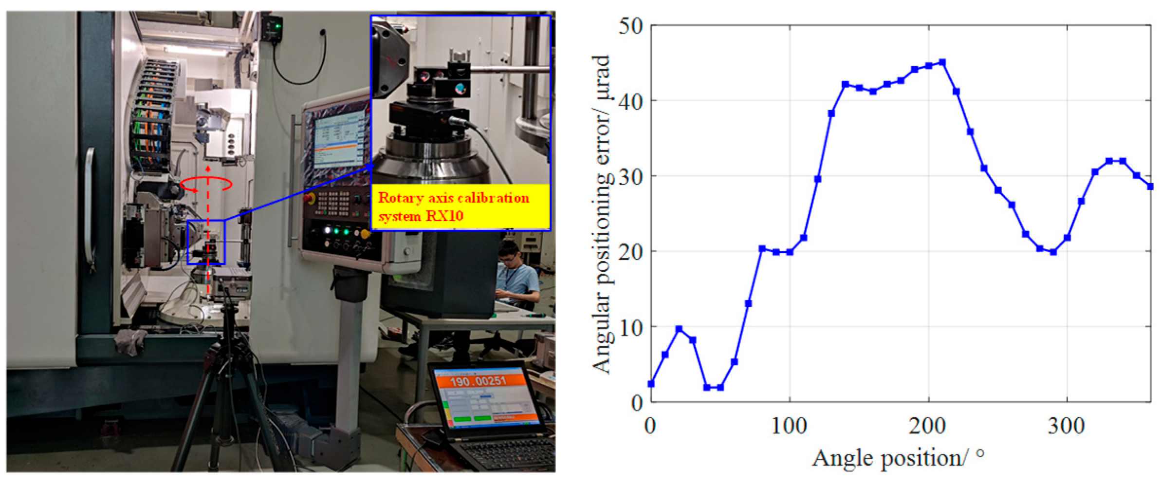
4. Geometric Error Measurement and Identification

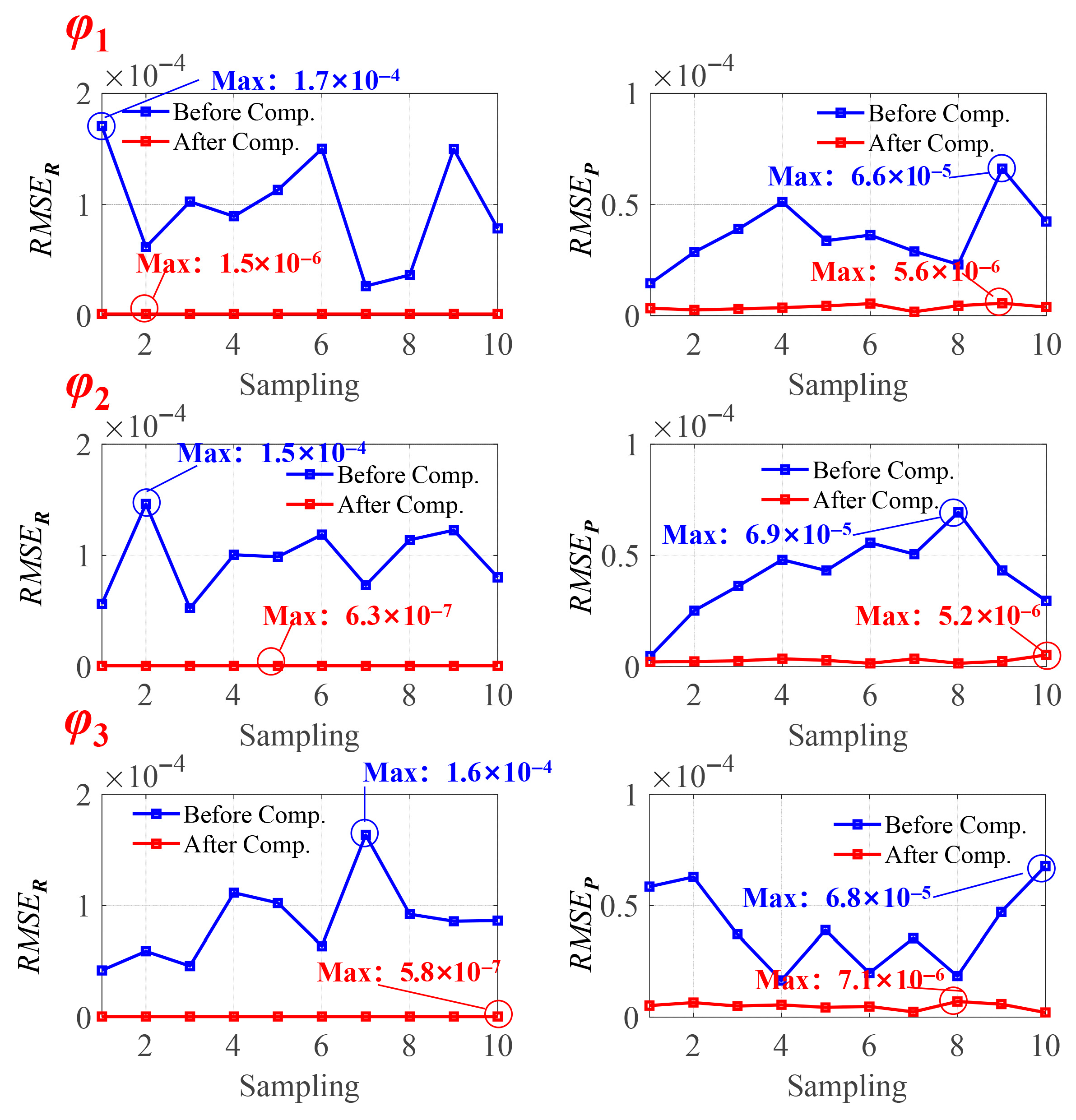
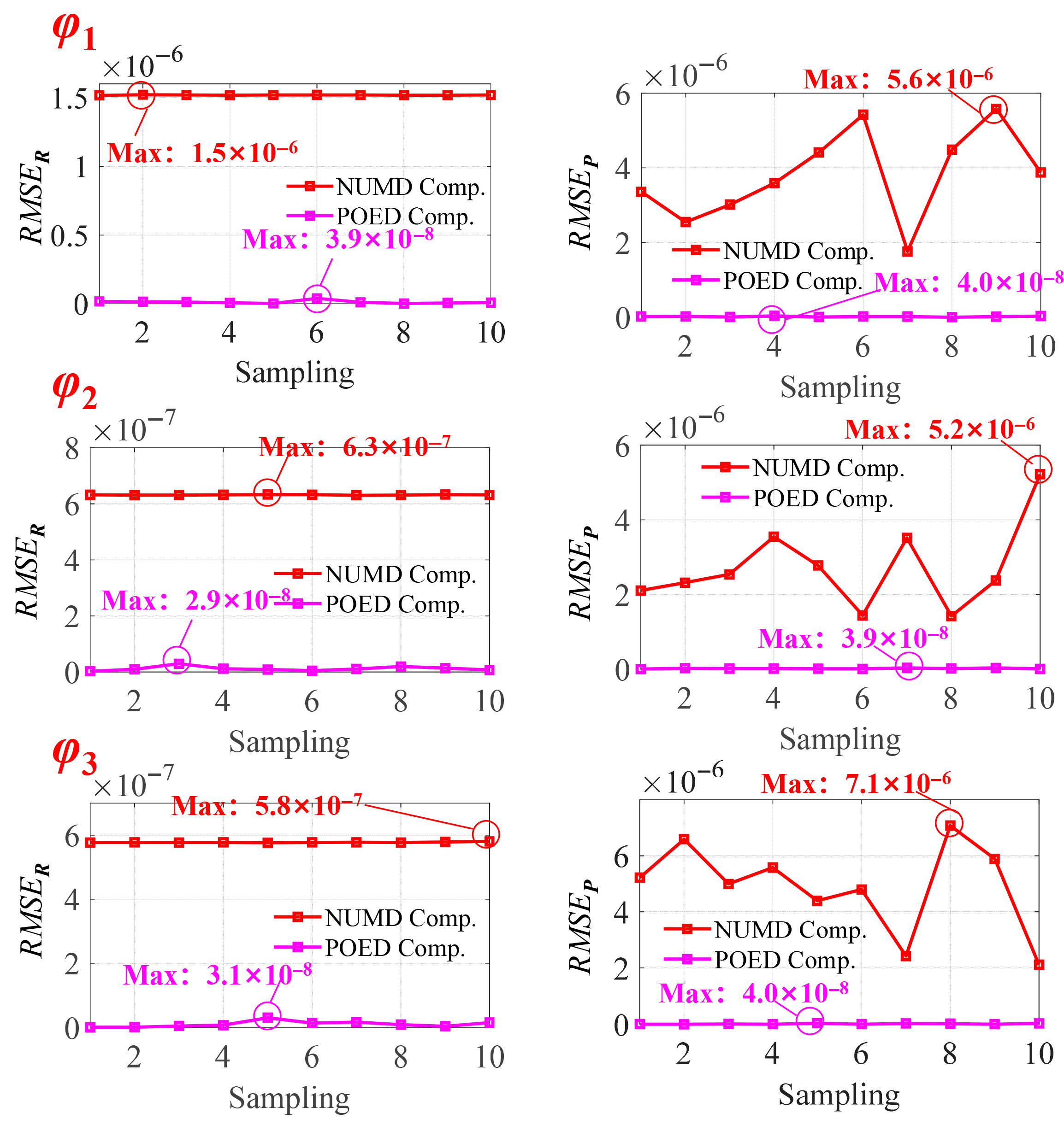
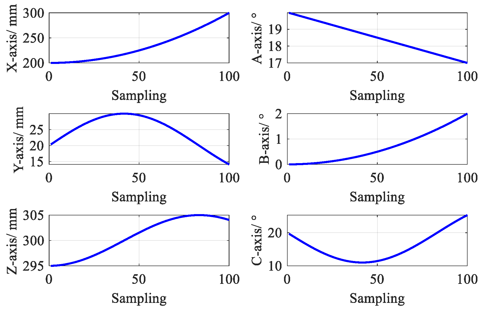
The multi-axis calibrator XM60 is used to detect all of the six PDGEs of the linear axis. The measurement processes and results of the geometric errors of the X-, Y-, and Z-axis are shown in Figure 7 and Figure 8. The three PIGEs, S_xy, S_xz, and S_yz, are measured using block and dial gauge by the workshop operators.

The direct measurement of the geometric errors of the rotary axis is much more difficult compared to the linear axis. In recent years, the double ball bar is used to identify the geometric errors in an indirect way. For the PIGEs, the circular tests were carried out at multi-height along the axis line of the rotary axis as shown in Figure 9. Depending on the center of the circle fitted by the least square method, the actual axis average line can be obtained [32], where H_i represents the installation height of the double ball bar relative to the reference plane.

In this way, the PIGEs of the A-axis and C-axis can be further identified depending on the definition in ISO 230-7 [33]. The measurement processes were shown in Figure 10, and, in total, eight and six circular tests were conducted along the axis line for the A-axis and C-axis, respectively.

For the A-axis, O₀, O₂₅, O₅₀, O₇₅, O₁₀₀, O₁₂₅, O₁₅₀, and O₁₇₅ represent the least square center of the circular trajectory at height from H1 to H8, where H1 and H8 represent the starting and ending positions along X-axis direction with distance of 175 mm. For the C-axis, O₀, O₅₀, O₁₀₀, O₁₅₀, O₂₀₅, and O₂₆₀ represent the least square center of the circular trajectory at height from H1 to H6, where H1 and H6 represent the starting and ending positions along the Z-axis direction with a distance of 260 mm. The obtained axis average lines of the A-axis and C-axis were shown in Figure 10. Correspondingly, the eight PIGEs of each axis can be calculated and summarized in

Table 5. Four identified PIGEs of A-axis and C-axis.

Error	δoyA	δozA	εozA	εoyA
PIGEs of A-axis	24.6 μm	78.5 μm	−441 μrad	623 μrad
Error	δoxC	δoyC	εoxC	εoyC
PIGEs of C-axis	0 μm	−1.4 μm	39.3 μrad	−50.7 μrad

. Analysis of the error distribution reveals that the A-axis exhibits significantly greater deviation compared to the C-axis, demonstrating the superior assembly accuracy of the latter. This discrepancy can be attributed to fundamental structural differences: the C-axis benefits from inherent symmetry in its design, while the A-axis’s suspended mounting configuration on the Z-axis, which additionally supports both B-axis and Y-axis components, introducing greater complexity that compromises its assembly precision.

The PDGE identification of rotary axis is relatively mature with DBB. In Ref. [34], a general identification method was proposed, which can construct appropriate measurement patterns for the A-axis and C-axis based on the rotary axis structure. Referring to this method, the error measurements and the identified PDGEs of the A-axis and C-axis are shown in Figure 11. For the angular positioning error of the A-axis, due to the structural limitation, the direct measurement and indirect identification are both difficult. As for the C-axis, the angular positioning error can be detected with rotary axis calibration device RX10 (Renishaw plc, Wotton-under-Edge, UK) with the laser interferometer XL80 (Renishaw plc, Wotton-under-Edge, UK), as shown in Figure 12.

5. Case Study

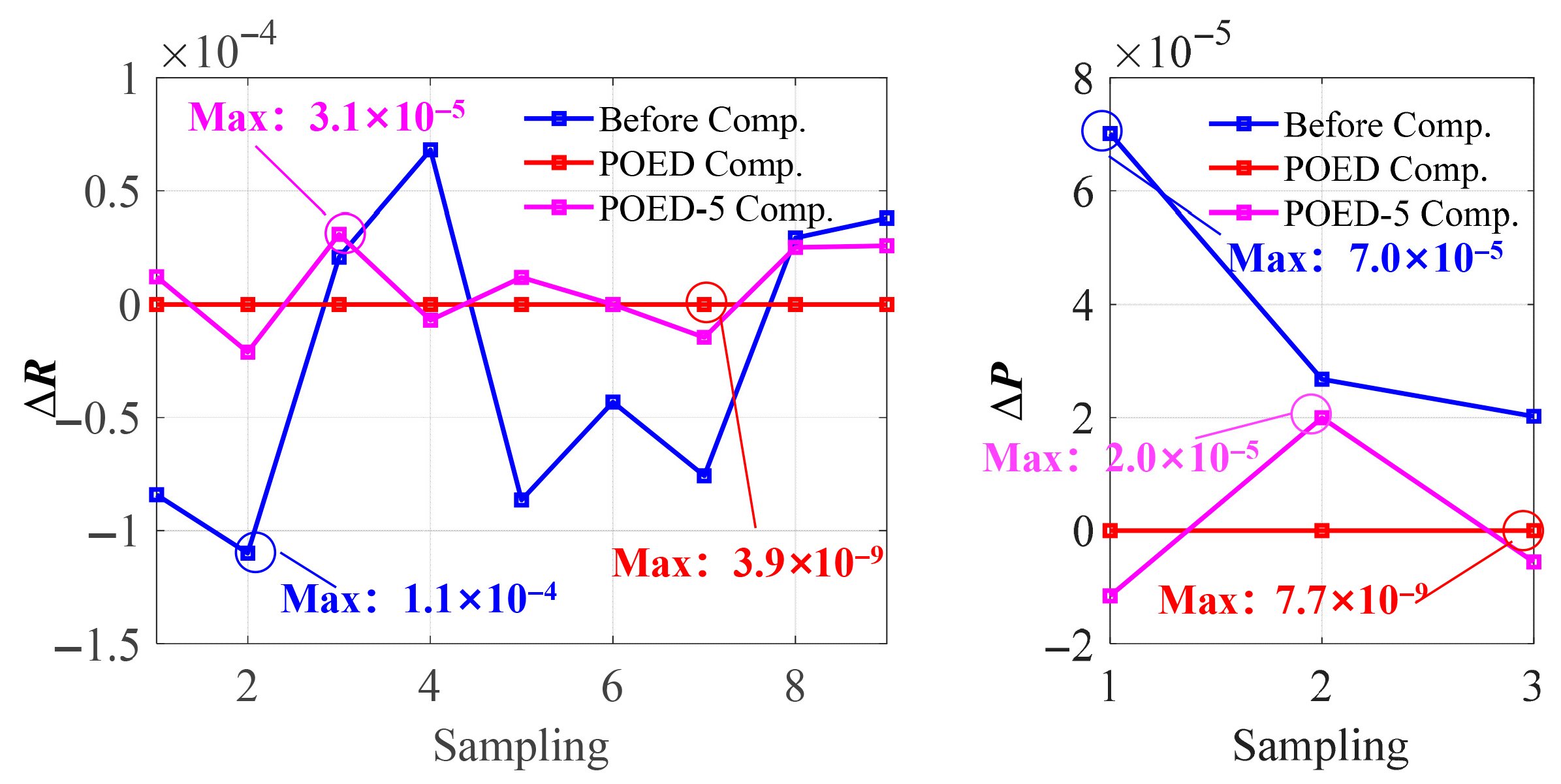
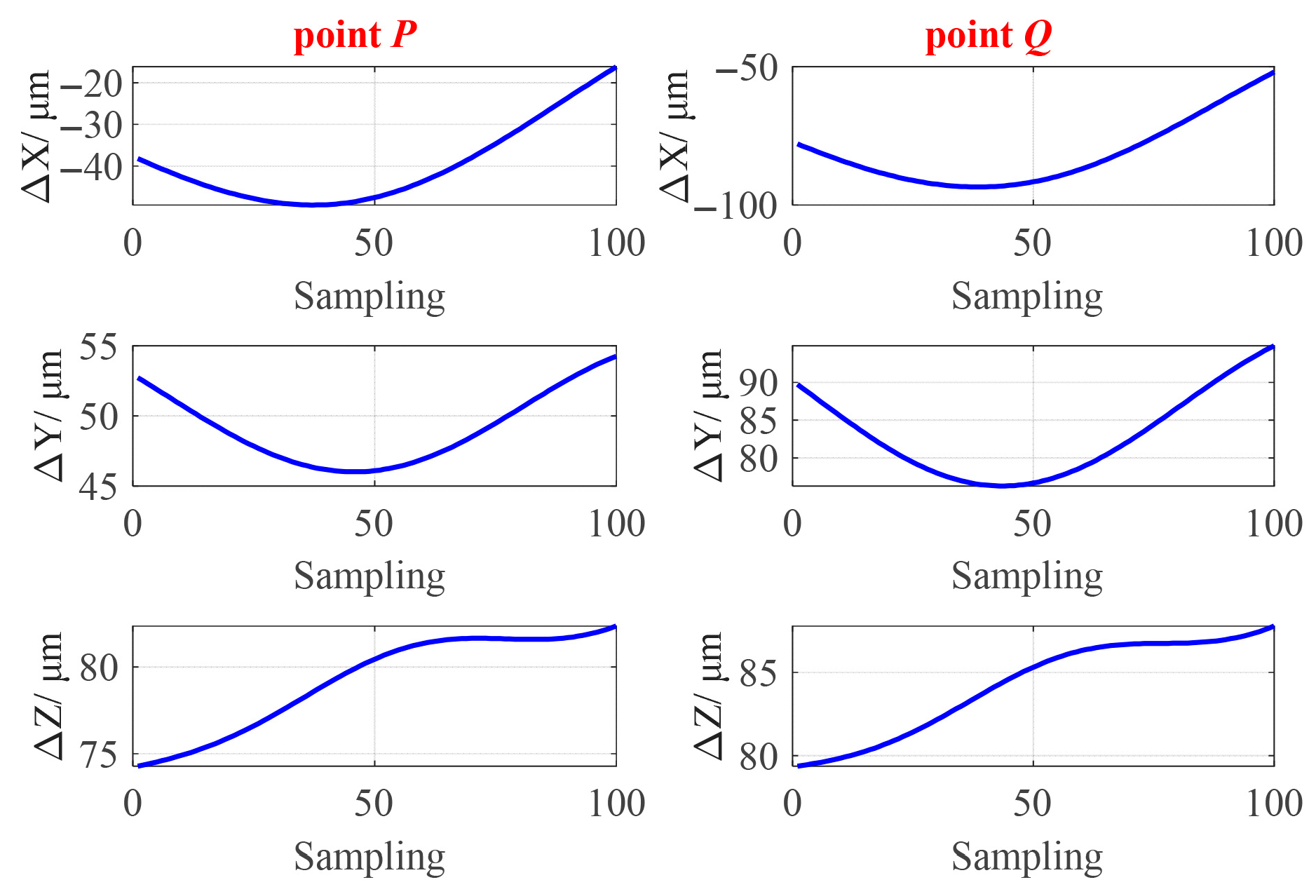
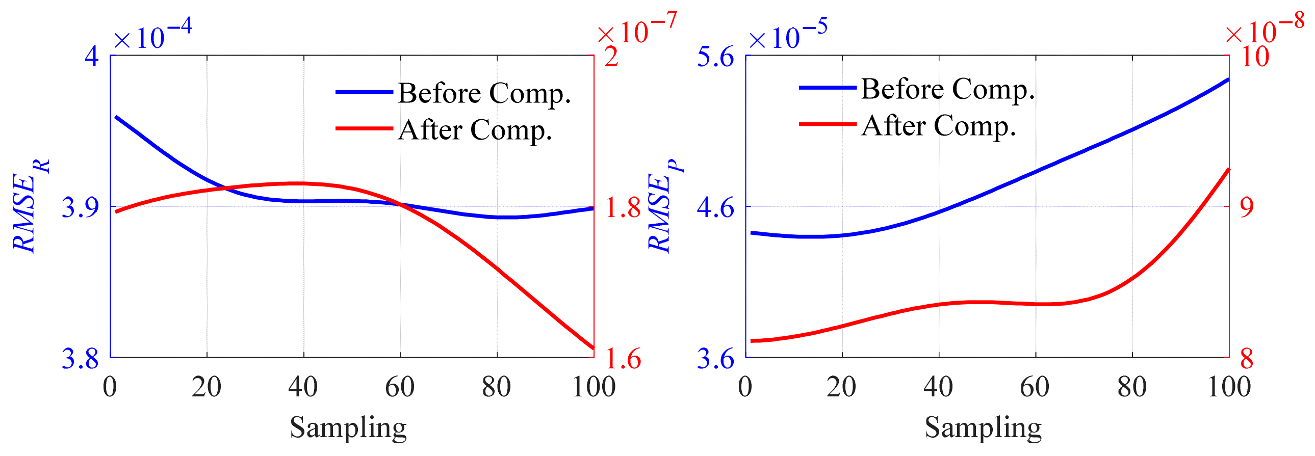
5.1. Geometry Error Compensation

The 40 geometric errors are fitted as functions of the axis motion and substituted into the volumetric error model of the grinding machine. Due to the structural limitation, it is difficult to directly detect the volumetric error caused by all the axis motions. Therefore, in this work, the volumetric error compensation was conducted and verified through the simulation in which two points were used to represent the tool–workpiece pose. The coordinates of the two points were set as P (10.000 mm, 50.000 mm, and 200.000 mm) and Q (30.000 mm, 100.000 mm, and 240.000 mm).

The theoretical axis motion command is preset in Figure 13. It is noted that because the established volumetric error model is the combination of two motion branches, the corresponding pose transformation is no longer based on the bed coordinate system.

Table 6. Position deviation of points P and Q.

Sampling	P/μm			Q/μm
	ΔX	ΔY	ΔZ	ΔX	ΔY	ΔZ
1	−38.2	52.7	74.3	−77.9	89.7	79.4
2	−38.7	52.5	74.3	−78.6	89.3	79.4
3	−39.2	52.3	74.4	−79.3	88.8	79.5
4	−39.7	52.1	74.5	−80.0	88.3	79.5
5	−40.2	51.9	74.5	−80.6	87.9	79.6
……	……	……	……	……	……	……
96	−19.1	53.7	82.0	−55.6	93.5	87.4
97	−18.3	53.8	82.1	−54.7	93.8	87.5
98	−17.6	54.0	82.2	−53.7	94.2	87.6
99	−16.9	54.1	82.3	−52.8	94.5	87.7
100	−16.2	54.3	82.4	−51.9	94.8	87.8

and Figure 14 show the position deviation between the actual coordinates and theoretical coordinates of points P and Q.

According to the proposed POED method, the compensation value of axis motion can be calculated, and the volumetric error is then compensated. The compensation performance indexes RSME_R and RSME_P of the motion transformation matrix are compared, as shown in Figure 15. The RMSEs of the ATM and PTM are reduced by three orders of magnitude, turning out that the compensation effect is remarkable.

Then, the position deviations of points P and Q after compensation are shown in Figure 16. The results show that the position deviations of both points can be well compensated. For example, the position deviation in X-direction of point P, ΔX ranges from −50 μm to 20 μm before compensation and narrows to 0–0.1 μm after compensation. The trajectories of P and Q before and after compensation are shown in Figure 17. The line segment connecting points P and Q can be regarded as a rigid body. After compensation, the PQ line segment almost completely coincides with the line segment at the theoretical location.

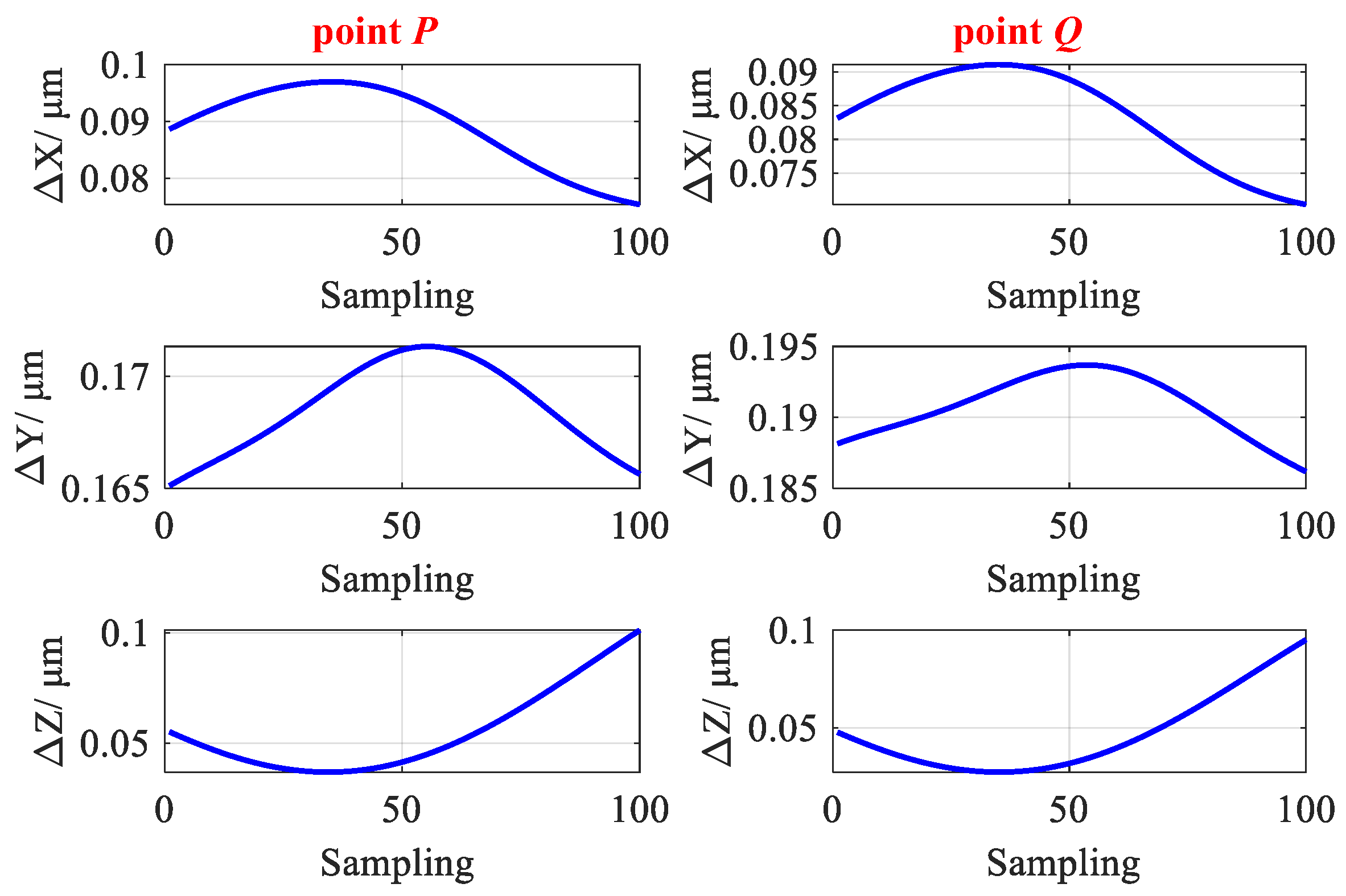
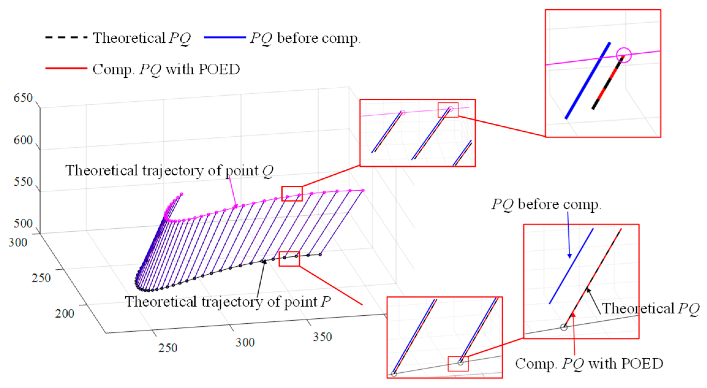
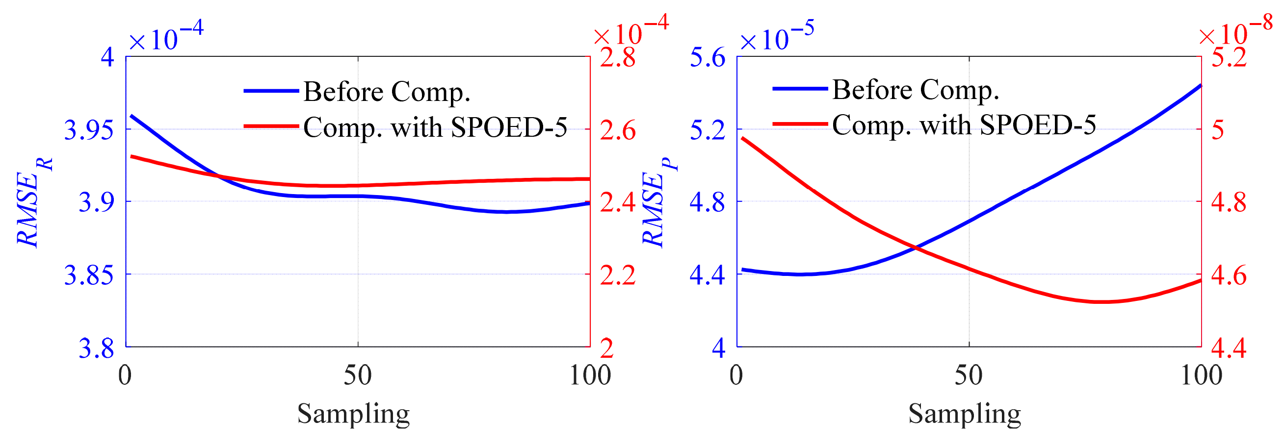
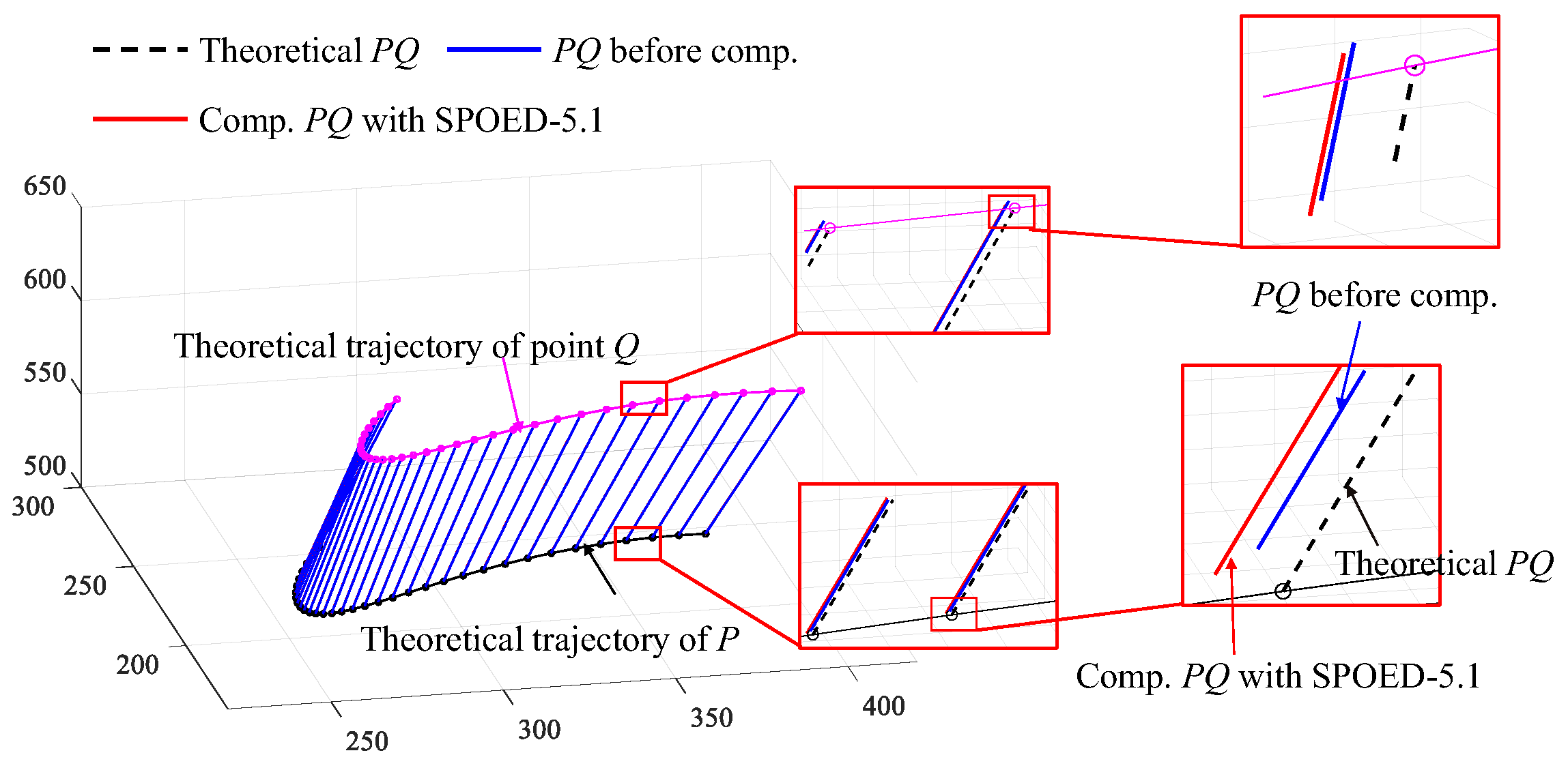
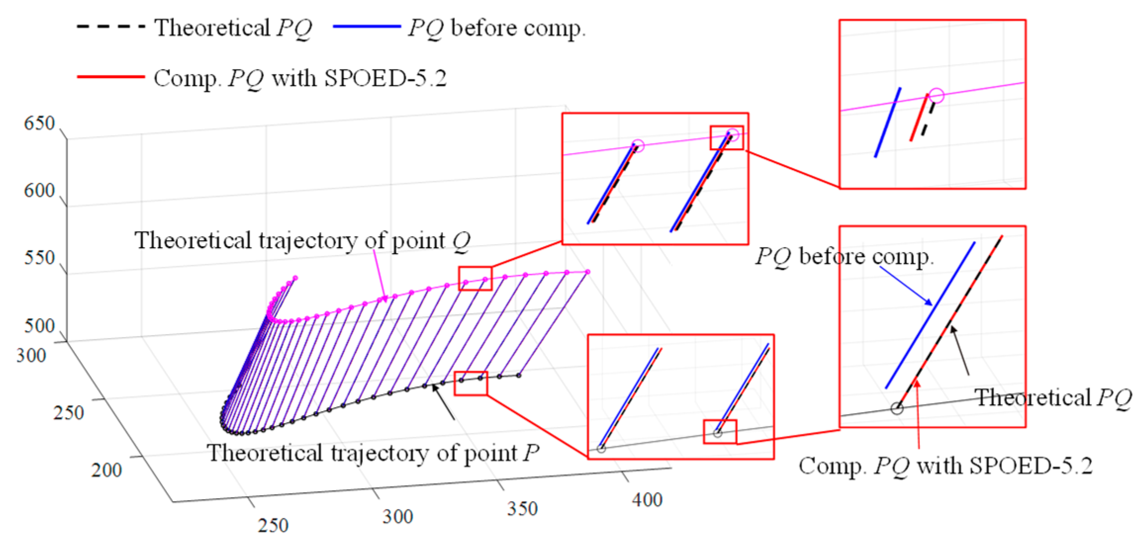
5.2. Step-by-Step Jacobi Compensation Under the Limitation of Compensation Motion Commands

When the compensation motion is limited, that is, the B-axis does not participate in the compensation motion, the volumetric error can only be compensated by the motion of the X-, Y-, Z-, A-, and C-axis. The volumetric error model is compensated with the SPODE-5 method. The RMSEs of ATM and PTM are shown in Figure 18. The value of RMSE_P after compensation is reduced by three orders of magnitude, which indicates that the compensation effect is obvious for PTM. However, the value of RMSE_R is generally smaller than that before compensation, but the order of magnitude is still 10⁻⁴. Compared with the compensation performance of tool–workpiece position error, the compensation performance of RMSE_R is weaker, because the A-axis and C-axis cannot completely compensate for the attitude error.

When the detailed coordinates of P and Q are not considered, the compensation method is denoted as SPOED-5.1. When the coordinates of P and Q are considered, the tool–workpiece position deviation is different at P and Q, and the position deviation ΔP₂ and ΔQ₂ of the two points can be calculated as shown in Equation (31). The compensation method is denoted as SPOED-5.2.

$$\left\{\begin{array}{l}\left[\begin{array}{c}\Delta {\mathit{P}}_2\\ 1\end{array}\right]={(E{T}_C\cdot T_C)}^{-1}\cdot E{T}_X\cdot T_X\cdot E{T}_Z\cdot T_Z\cdot E{T}_A\cdot T_A\cdot E{T}_Y\cdot T_Y\cdot E{T}_B\cdot T_B\cdot \left[\begin{array}{c}{\mathit{P}}_0\\ 1\end{array}\right]\\ -{(T_C)}^{-1}\cdot T_X\cdot T_Z\cdot T_A\cdot T_Y\cdot T_B\cdot \left[\begin{array}{c}{\mathit{P}}_0\\ 1\end{array}\right]\\ \left[\begin{array}{c}\Delta {\mathit{Q}}_2\\ 1\end{array}\right]={(E{T}_C\cdot T_C)}^{-1}\cdot E{T}_X\cdot T_X\cdot E{T}_Z\cdot T_Z\cdot E{T}_A\cdot T_A\cdot E{T}_Y\cdot T_Y\cdot E{T}_B\cdot T_B\cdot \left[\begin{array}{c}{\mathit{Q}}_0\\ 1\end{array}\right]\\ -{(T_C)}^{-1}\cdot T_X\cdot T_Z\cdot T_A\cdot T_Y\cdot T_B\cdot \left[\begin{array}{c}{\mathit{Q}}_0\\ 1\end{array}\right]\end{array}\right.$$

(31)

The SPOED-5.2 method can only ensure that the position deviation of one point is completely compensated, and other points are generated with the compensation motion of the point. It is assumed that point P is the target point and the position deviation of point P is compensated. The position deviations of the P and Q points with compensation SPOED-5.1 and SPOED-5.2 are shown in Figure 19 and

Table 7. Compensation performance using SPOED-5.1 and SPOED-5.2.

Directions		Before		POED (6-Axis Comp.)		SPOED-5.1		SPOED-5.2
		Max	Range	Max	Range	Max	Range	Max	Range
X	ΔXP	49.4	33.2	0.10	0.02	95.7	9.9	0.06	0.02
	ΔXQ	93.5	41.6	0.09	0.02	123.2	15.2	27.6	5.4
Y	ΔYP	54.3	8.3	0.17	0.006	64.2	22.3	0.03	0.01
	ΔYQ	94.8	18.5	0.19	0.008	81.0	26.4	17.0	4.3
Z	ΔZP	82.4	8.0	0.10	0.06	9.7	2.4	0.03	0.01
	ΔZQ	87.8	8.4	0.10	0.07	17.0	3.3	7.2	0.8
Mean value		—	19.7	—	0.03	—	13.3	—	1.8

, where Max represents the maximum absolute value of the position deviation, relative to the theoretical position, and Range represents the variation range of position deviation. In addition, the six-axis compensation method POED, is compared, in which the detailed point coordinates are not considered.

As a reference method using six-axis compensation motions, the POED method can achieve excellent results, effectively reducing the maximum position deviation Max and the deviation range Range. The mean value of the ranges can be reduced from 19.7 μm to 0.03 μm. As previously discussed, when using five-axis decoupling methods, the compensation performance is weaker than that of the six-axis method. After compensation, the SPOED-5.1 method reduces the deviation ranges in X and Z direction, while it failed to the compensate the maximum deviations, where some of the deviations even become larger like ΔX_P, ΔX_Q, and ΔY_P. The mean value of the ranges is 13.3 μm, showing a certain degree of compensation effect compared to the original value of 19.7 μm. As for the SPOED-5.2 method, the position deviations as well as the deviation ranges of points P and Q are well compensated, and the mean value of the ranges is 1.8 μm, which is already very close to the method using six-axis compensation motions. Due to the compensation motion commands are calculated depending on the position deviation of point P, the compensation performance of point P is better than that of point Q.

Draw the trajectories of point P and point Q before and after compensation with SPOED-5.1 and SPOED-5.2, as shown in Figure 20 and Figure 21, respectively. With SPOED-5.1 compensation, although indexes such as RMSE_R and RMSE_P are obviously reduced, the SPOED-5.1 method cannot compensate for the absolute position deviations of point P and point Q and make the PQ line fall on the theoretical location, while with SPOED-5.2 compensation, the actual trajectory of point P is almost consistent with the theoretical location, and the PQ line close to the point P almost overlaps with the theoretical PQ location.

In general, the six-axis compensation method POED can fully compensate both position and attitude errors, offering a comprehensive solution with excellent compensation performance across all points, regardless of specific point coordinates. When compensation motion is limited, the step-by-step SPOED-5.2 method can effectively compensate for the position deviation of a specific point, even with incomplete compensation of the attitude deviation. This approach also supports volumetric error compensation for common five-axis machining tools.

6. Conclusions

This work focuses on the inverse solution of the volumetric error of the six-axis gear grinding machine and proposes a Jacobian matrix to decouple the volumetric error model. Some conclusion can be summarized as follows.

(1) Using the screw theory, the forward kinematics model of the six-axis gear grinding machine and the volumetric error model considering 41 geometric errors are established. The Jacobian matrix decoupling method POED is proposed in an analytical derivation way, which can compensate for all the errors in full degree of freedom.

(2) In total, 40 geometric errors (without the angular positioning error of the A-axis) of the grinding machine are directly measured and indirectly identified with laser interferometer and double ball bar. Additionally, these errors are used for the subsequent volumetric error modeling process.

(3) For the situation where the compensation motion command is limited, an improved SPOED-5.2 method is proposed by combining the coordinates of the target point, and the mean value of the comprehensive error ranges can be reduced from 19.7 μm to 1.8 μm, which can achieve a significant compensation for the attitude and position deviation.

References

1. Gao, W.; Ibaraki, S.; Donmez, M.A.; Kono, D.; Mayer, J.R.R.; Chen, Y.-L.; Szipka, K.; Archenti, A.; Linares, J.-M.; Suzuki, N. Machine tool calibration: Measurement, modeling, and compensation of machine tool errors. Int. J. Mach. Tools Manuf. 2023, 187, 104017. [Google Scholar] [CrossRef]
2. Niu, P.; Cheng, Q.; Liu, Z.; Chen, C.; Zhao, Y.; Li, Y.; Qi, B. Multi-objective optimal tolerance allocation design of machine tool based on NSGA-II algorithm and thermal characteristic analysis. Proc. Inst. Mech. Eng. Part B J. Eng. Manuf. 2025. [Google Scholar] [CrossRef]
3. Ding, W.; Zhu, X.; Huang, X. Effect of servo and geometric errors of tilting-rotary tables on volumetric errors in five-axis machine tools. Int. J. Mach. Tools Manuf. 2016, 104, 37–44. [Google Scholar] [CrossRef]
4. Xiang, S.; Altintas, Y. Modeling and compensation of volumetric errors for five-axis machine tools. Int. J. Mach. Tools Manuf. 2016, 101, 65–78. [Google Scholar] [CrossRef]
5. Yang, J.; Altintas, Y. Generalized kinematics of five-axis serial machines with non-singular tool path generation. Int. J. Mach. Tools Manuf. 2013, 75, 119–132. [Google Scholar] [CrossRef]
6. Zhang, H.; Cheng, G.; Shan, X.; Guo, F. Kinematic accuracy research of 2(3HUS+S) parallel manipulator for simulation of hip joint motion. Robotica 2018, 36, 1386–1401. [Google Scholar] [CrossRef]
7. Fu, G.; Fu, J.; Gao, H.; Yao, X. Squareness error modeling for multi-axis machine tools via synthesizing the motion of the axes. Int. J. Adv. Manuf. Technol. 2016, 89, 2993–3008. [Google Scholar] [CrossRef]
8. Wang, H.; Jiang, X.G. Identification and compensation of position independent geometric errors of dual rotary axes for hybrid-type five-axis machine tool based on unit dual quaternions. Measurement 2023, 211, 112587. [Google Scholar] [CrossRef]
9. Wang, H.; Jiang, X. Geometric error identification of five-axis machine tools using dual quaternion. Int. J. Mech. Sci. 2022, 229, 107522. [Google Scholar] [CrossRef]
10. Zhu, S.; Ding, G.; Qin, S.; Lei, J.; Zhuang, L.; Yan, K. Integrated geometric error modeling, identification and compensation of CNC machine tools. Int. J. Mach. Tools Manuf. 2012, 52, 24–29. [Google Scholar] [CrossRef]
11. Rahman, M.; Heikkala, J.; Lappalainen, K. Modeling, measurement and error compensation of multi-axis machine tools. Part I: Theory. Int. J. Mach. Tools Manuf. 2000, 40, 1535–1546. [Google Scholar] [CrossRef]
12. Yang, J.; Mayer, J.R.R.; Altintas, Y. A position independent geometric errors identification and correction method for five-axis serial machines based on screw theory. Int. J. Mach. Tools Manuf. 2015, 95, 52–66. [Google Scholar] [CrossRef]
13. Wan, H.; Chen, S.; Zheng, T.; Jiang, D.; Zhang, C.; Yang, G. Piecewise modelling and compensation of geometric errors in five-axis machine tools by local product of exponentials formula. Int. J. Adv. Manuf. Technol. 2022, 121, 2987–3004. [Google Scholar] [CrossRef]
14. Wang, S.M.; Ehmann, K.F. Measurement methods for the position errors of a multi-axis machine. Part 1: Principles and sensitivity analysis. Int. J. Mach. Tools Manuf. 1999, 39, 951–964. [Google Scholar] [CrossRef]
15. Wang, S.M.; Ehmann, K.F. Measurement methods for the position errors of a multi-axis machine. Part 2. applications and experimental results. Int. J. Mach. Tools Manuf. 1999, 39, 1485–1505. [Google Scholar] [CrossRef]
16. Hu, T.; Wang, W.; Jiang, Y.; Mi, L.; Yao, X. An integrated methodology of volumetric error modeling, validation, and compensation for horizontal machining centers. Int. J. Adv. Manuf. Technol. 2021, 115, 1445–1459. [Google Scholar] [CrossRef]
17. Cui, G.; Lu, Y.; Li, J.; Gao, D.; Yao, Y. Geometric error compensation software system for CNC machine tools based on NC program reconstructing. Int. J. Adv. Manuf. Technol. 2012, 63, 169–180. [Google Scholar] [CrossRef]
18. Hsu, Y.Y.; Wang, S.S. A new compensation method for geometry errors of five-axis machine tools. Int. J. Mach. Tools Manuf. 2007, 47, 352–360. [Google Scholar] [CrossRef]
19. Peng, F.Y.; Ma, J.Y.; Wang, W.; Duan, X.Y.; Sun, P.P.; Yan, R. Total differential methods based universal post processing algorithm considering geometric error for multi-axis NC machine tool. Int. J. Mach. Tools Manuf. 2013, 70, 53–62. [Google Scholar] [CrossRef]
20. Chen, J.; Lin, S.; He, B. Geometric error compensation for multi-axis CNC machines based on differential transformation. Int. J. Adv. Manuf. Technol. 2013, 71, 635–642. [Google Scholar] [CrossRef]
21. Mir, Y.A.; Mayer, J.R.R.; Fortin, C. Tool path error prediction of a five-axis machine tool with geometric errors. Proc. Inst. Mech. Eng. Part B J. Eng. Manuf. 2002, 216, 697–712. [Google Scholar] [CrossRef]
22. Rahman, M.M.; Mayer, J.R.R. Five axis machine tool volumetric error prediction through an indirect estimation of intra- and inter-axis error parameters by probing facets on a scale enriched uncalibrated indigenous artefact. Precis. Eng.-J. Int. Soc. Precis. Eng. Nanotechnol. 2015, 40, 94–105. [Google Scholar] [CrossRef]
23. Givi, M.; Mayer, J.R.R. Volumetric error formulation and mismatch test for five-axis CNC machine compensation using differential kinematics and ephemeral G-code. Int. J. Adv. Manuf. Technol. 2014, 77, 1645–1653. [Google Scholar] [CrossRef]
24. Fu, G.; Fu, J.; Xu, Y.; Chen, Z.; Lai, J. Accuracy enhancement of five-axis machine tool based on differential motion matrix: Geometric error modeling, identification and compensation. Int. J. Mach. Tools Manuf. 2015, 89, 170–181. [Google Scholar] [CrossRef]
25. Fu, G.; Fu, J.; Shen, H.; Xu, Y.; Jin, Y. Product-of-exponential formulas for precision enhancement of five-axis machine tools via geometric error modeling and compensation. Int. J. Adv. Manuf. Technol. 2015, 81, 289–305. [Google Scholar] [CrossRef]
26. Ding, S.; Chen, Z.; Zhang, H.; Yang, W.; Wu, W.; Song, A. Gear evaluation deviations-based crucial geometric error identification of five-axis CNC gear form grinding process. J. Manuf. Process. 2023, 99, 663–675. [Google Scholar] [CrossRef]
27. Xia, C.; Wang, S.; Wang, S.; Ma, C.; Xu, K. Geometric error identification and compensation for rotary worktable of gear profile grinding machines based on single-axis motion measurement and actual inverse kinematic model. Mech. Mach. Theory 2021, 155, 104042. [Google Scholar] [CrossRef]
28. Tang, Z.; Zhou, Y.; Wang, S.; Zhu, J.; Tang, J. An innovative geometric error compensation of the multi-axis CNC machine tools with non-rotary cutters to the accurate worm grinding of spur face gears. Mech. Mach. Theory 2022, 169, 104664. [Google Scholar] [CrossRef]
29. Liu, Y.; Hong, R.; Lin, X.; Zhang, H.; Zhang, H.; Pan, Y. An identification method for a large-scale helical gear grinding process based on analysis of geometric errors. J. Manuf. Process. 2024, 121, 51–62. [Google Scholar] [CrossRef]
30. Zhang, L.; Cheng, L.; Li, J.; Ke, Y. Modeling and compensation of volumetric errors for a six-axis automated fiber placement machine based on screw theory. Proc. Inst. Mech. Eng. Part B J. Eng. Manuf. 2021, 235, 6940–6955. [Google Scholar] [CrossRef]
31. Zhang, K.; He, X.; Li, R.; Huang, P.; Feng, B.; Feng, H.; Huang, L.; Peng, Y. A novel method of volumetric error compensation for aspherical grinding machine considering error coupling effect and compensation strategy. Int. J. Adv. Manuf. Technol. 2025, 137, 3673–3693. [Google Scholar] [CrossRef]
32. Kai, X.; Zheyu, L.; Guolong, L.; Liuqing, D.; Jianwei, J. An improved robust identification method for position independent geometric errors of the swing axis of the gear grinding machine. Int. J. Adv. Manuf. Technol. 2024, 135, 4963–4973. [Google Scholar] [CrossRef]
33. ISO 230–7; Test Code for Machine Tool-Part 7: Geometric Accuracy of Axes of Rotation. ISO: Geneva, Switzerland, 2006.
34. Xu, K.; Li, G.L.; Li, Z.Y.; Dong, X.; Xia, C.J. A general identification method for position-dependent geometric errors of rotary axis with single-axis driven. Int. J. Adv. Manuf. Technol. 2021, 112, 1171–1191. [Google Scholar] [CrossRef]
Figure 1. Structure diagram of the gear grinding machine.
Actuators 14 00374 g001
Figure 2. Numerical solution of the volumetric error model.
Actuators 14 00374 g002
Figure 3. RMSE comparison before and after compensation.
Actuators 14 00374 g003
Figure 4. RMSEs before and after compensation under 3 sets of axis motion commands.
Actuators 14 00374 g004
Figure 5. Compensation performance using 5 axes with the POED-5.
Actuators 14 00374 g005
Figure 6. Flow chart of step-by-step decoupling.
Actuators 14 00374 g006
Figure 7. Linear positioning error measurement of X-, Y-, and Z-axis using XM60 multi-axis calibrator.
Actuators 14 00374 g007
Figure 8. Measurement results of 6 PDGEs of X-, Y-, and Z-axis.
Actuators 14 00374 g008
Figure 9. Circular tests at different heights.
Actuators 14 00374 g009
Figure 10. Measurements for PIGEs identification of A-axis and C-axis.
Actuators 14 00374 g010
Figure 11. Measurement for PDGE identification of A-axis and C-axis.
Actuators 14 00374 g011
Figure 12. Direct measurement and result of the angular positioning error of C-axis.
Actuators 14 00374 g012
Figure 13. Theoretical axis motion commands.
Actuators 14 00374 g013
Figure 14. Position deviation of P and Q before compensation.
Actuators 14 00374 g014
Figure 15. Compensation performance of the ATM and PTM using POED method.
Actuators 14 00374 g015
Figure 16. Position error of P and Q after compensation.
Actuators 14 00374 g016
Figure 17. Volumetric trajectory of points P and Q before and after error compensation.
Actuators 14 00374 g017
Figure 18. Compensation performance of the ATM and PTM using POED-5 method.
Actuators 14 00374 g018
Figure 19. Position deviations of P and Q after compensation.
Actuators 14 00374 g019
Figure 20. Trajectories of points P and Q before and after compensation using SPOED-5.1.
Actuators 14 00374 g020
Figure 21. Trajectories of points P and Q before and after compensation using SPOED-5.2.
Actuators 14 00374 g021