PD-like Consensus Tracking Algorithm for Discrete Multi-Agent Systems with Time-Varying Reference State Under Binary-Valued Communication

Abstract

In this paper, a new consensus tracking control algorithm is proposed for discrete multi-agent systems under binary communication with noise and a time-varying reference state. Unlike previous studies, the leader’s reference state is time-varying and convergent. Each agent estimates its neighbors’ states using a recursive projection algorithm based on noisy binary-valued information. The controller design incorporates both the error between the current and estimated states and the rate of change of the estimated state, resulting in a proportional–derivative-like algorithm (PD-like algorithm). The algorithm achieves consensus tracking with a convergence rate of $O(1/t^{\epsilon })$ under certain conditions. Finally, numerical simulations demonstrate the algorithm’s effectiveness and validate the theoretical results.

1. Introduction

Multi-agent systems (MASs) consist of multiple interacting agents and are widely applied in areas such as autonomous vehicle platooning, multi-UAV systems, microgrid frequency control, and other domains [1,2,3]. The consensus control problem is one of the core issues in MAS, aiming to design distributed controllers to make the states of all agents converge to a consensus. The theoretical study of consensus problems began in [4], where A. Jadbabaie et al. provided a theoretical explanation for the phenomenon observed in the Vicsek model [5] using graph connectivity, thus improving the coordination theory based on the nearest neighbor rule in MASs. In [6], R. Olfati-Saber et al. used the Laplacian matrix to study the consensus problem in MASs, providing a consensus analysis framework based on graph theory. Ref. [7] pointed out that under dynamic interaction topologies, if the union of interaction graphs has spanning trees frequently enough during certain time periods, MASs can asymptotically reach consensus, and the restrictions on weighting factors are relaxed. These laid the theoretical foundation for subsequent research on consensus in MAS.

In the consensus tracking control problem of MASs, leader-following consensus is an important cooperative control strategy. Ref. [8] studied the problem of achieving finite-time leader-following consensus in second-order multi-agent systems with both fixed and switching topologies. For situations where the leader’s state information cannot be directly obtained, ref. [9] proposed a tracking control protocol based on distributed observers using relative output measurements and information received from neighbors. Ref. [10] combined neighbor-based feedback control laws and dynamic estimation rules with Lyapunov stability analysis to investigate the consensus problem in MASs with an active leader and variable topologies.

With the practical application of MAS, the influence of noise such as sensor noise, channel fading, and electromagnetic interference on measurement and information communication cannot be ignored. Ref. [11] introduced a stochastic approximation algorithm for models with noisy measurements and proposed to combine the decay property of the stochastic Lyapunov function with the so-called invariance direction to achieve convergence analysis. Ref. [12] proposed a new velocity decomposition technique for noisy measurements and time-varying directed topologies and designed a distributed estimation algorithm based on it. Furthermore, with limited communication bandwidth resources, quantized communication has been introduced to improve communication efficiency among MASs. The study of quantized consensus began in [13], where each agent’s state was set as an integer, and a quantized gossip algorithm was proposed for the distributed averaging problem to achieve quantized consensus. Quantized communication has increasingly attracted the interest of researchers. Refs. [14,15,16,17] used different types of quantizers to study consensus problems.

However, there is relatively little research on binary communication, as a special form of quantized communication, in MASs. However, its simplicity, extremely low communication bandwidth requirements, and strong anti-interference ability have attracted many researchers. Refs. [18,19] study system identification problems under binary-valued observations and cyber-attacks. Ref. [20] proposed a two-time-scale consensus protocol for consensus problems with random noise and binary measurements under undirected and fixed topologies. However, the state estimation and control in it are carried out alternately. Inspired by the recursive projection algorithm, refs. [21,22] proposed a new consensus algorithm that can simultaneously perform state estimation and control and update the state in real time, considering noisy measurement and binary quantizers. The convergence rate of this algorithm is $O(1/t)$, which is faster than that in [20]. Ref. [23] further explored the consensus tracking problem in systems with time-invariant leaders under directed topologies. In this paper, the leader’s state discussed is time-varying, which is more challenging than in [22]. Meanwhile, in [24], the authors separately investigated the cases of a convergent leader and bounded leader. Decaying gains and constant gains in the control algorithms are designed for the two cases, respectively.

In this paper, the state of the leader is time-varying, and the uniform boundedness of the agent’s time-varying state cannot be guaranteed, requiring a reanalysis of its uniform boundedness properties. This increases the difficulty of analysis compared with the constant leader in Reference [23]. Moreover, most of the consensus algorithms with binary-valued communication only use proportional (P-like) control strategies based on the estimated states of neighbors. For consensus tracking problems with accurate information of neighbors, PD-like algorithms were designed in [25,26]. In this paper, a PD-like algorithm is introduced, taking into account the rate of change of the estimated state of the agents’ neighbors. How to analyze the influence of the derivative term on consensus error is more challenging.

The contributions of this paper are as follows:

• This paper proposes a novel online algorithm consisting of estimation and control for the consensus tracking problem with a time-varying reference state and binary-valued communication. In the estimation part, the recursive projection algorithm (RPA) is used to deal with binary-valued observations. In the control part, a differential term is added to track the varying of neighbors in addition to a proportional term, which results in a PD-like algorithm.
• Due to the introduction of differential terms, the PD-like algorithm increases the complexity of convergence analysis. The differential terms describe an estimate of the rate of change of the neighbors. Using the properties of the estimation algorithm, the differential term can be handled using the rate of change of the leader. If the state of the leader is convergent, it is proved that the followers can asymptotically track the leader using a dual Lyapunov function analysis framework constructed based on the estimation and tracking control.
• The PD-like algorithm has significant advantages in terms of convergence speed. It introduces the difference in state estimation in the control input and integrates the recursive projection estimation and differential feedback mechanisms, compensating for the loss of quantized information and enhancing the system’s adaptability to dynamic leaders. This enables the system to adjust its own state quickly and accelerate the convergence speed towards the leader’s state. Moreover, through theoretical analysis, it can be seen that the convergence rate of the algorithm depends on the rate of change of the leader. Compared with algorithms that only use proportional control strategies in [24], the convergence rate of this algorithm is faster, which ensures that the multi-agent system can quickly achieve consensus tracking with binary-valued communication.

The remainder of this paper is structured as follows. Nomenclature summarizes some important symbols. Section 2 describes the consensus tracking control problem with binary-valued communication. Section 3 presents the consensus tracking control algorithm. Section 4 provides the main conclusions of the algorithm, including convergence and the convergence rate. Section 5 verifies the effectiveness of the theory through simulation. Section 6 summarizes this paper and looks ahead to future work.

2. Problem Formulation

Consider a discrete-time multi-agent system consisting of n agents:

$$\begin{array}{c}\hfill x_i(t+1)=x_i\left(t\right)+u_i\left(t\right),i=1,\dots ,n,\end{array}$$

(1)

where $x_i\left(t\right)\in \mathbb{R}$ represents the state of agent i at time t, and $u_i\left(t\right)\in \mathbb{R}$ is the corresponding control input. This system also includes a leader agent $n+1$, whose state is $x_{n+1}\left(t\right)$ and is expressed as follows:

$$\begin{array}{c}\hfill x_{n+1}(t+1)=x_{n+1}\left(t\right)+u_{n+1}\left(t\right),\end{array}$$

(2)

where $u_{n+1}\left(t\right)$ is the rate of change of the leader’s state. The remaining n agents are called followers. So, the vector update equation of this system is as follows:

$$\begin{array}{c}\hfill X(t+1)=X\left(t\right)+U\left(t\right),t=1,2,\dots \end{array}$$

(3)

with $X\left(t\right)={\left[x_1\left(t\right),\dots ,x_{n+1}\left(t\right)\right]}^T$. Let $g\left(t\right)=u_{n+1}\left(t\right)$ and $U\left(t\right)={\left[u_1\left(t\right),\dots ,u_n\left(t\right),g\left(t\right)\right]}^T$.

Consider that the multi-agent system is represented by a directed topological network structure $G=(N,E)$, where $N=\{1,2,\cdots ,n+1\}$ is the set of nodes, and each node corresponds to an agent. $E=N\times N$ is the set of edges, which represent the channels for information interaction among agents. Matrix $A={\left(a_{ij}\right)}_{(n+1)\times (n+1)}$ is the adjacency matrix of topology G. If there is an edge from agent j to agent i, which means that agent i can directly obtain information from agent j, then $a_{ij}=1$, and agent j is called a neighbor of agent i, denoted as $j\in N_i$; otherwise, $a_{ij}=0$, and agent j is not a neighbor of agent i. $D=diag(d_1,d_2,\cdots ,d_{n+1})$ is the degree matrix, where $d_i$ represents the number of neighbors of agent i. Specifically, since the leader cannot receive feedback from any follower, for adjacency matrix A, we have $a_{(n+1)j}=0$, $j=1,2,\cdots ,n$, and $d_{(n+1)}=0$. The Laplacian matrix of the directed graph is $L=D-A$.

When agent i receives information from its neighbor agent j, it is affected by random noise, and its observed value is as follows:

$$\begin{array}{c}\hfill \left\{\begin{array}{c}{y}_{ij}\left(t\right)=x_j\left(t\right)+{\sigma }_{ij}\left(t\right),j=1,2,\dots ,n+1,\hfill \\ s_{ij}\left(t\right)=I_{\{y_{ij}\left(t\right)\le C\}},j\in N_i,\hfill \end{array}\right.\end{array}$$

(4)

where $N_i$ is the set of all neighbors of agent i, $x_j\left(t\right)$ is the state of agent j at time t, ${\sigma }_{ij}\left(t\right)\in \mathbb{R}$ is the communication noise, $y_{ij}\left(t\right)\in \mathbb{R}$ is the unmeasurable output, C is the binary sensor threshold, and $s_{ij}\left(t\right)$ is the binary information obtained by agent i from neighbor agent j. $I_{\{.\}}$ is an indicative function, defined as

$$\begin{array}{c}\hfill I_{\{v\in V\}}=\left\{\begin{array}{c}1,\mathrm{if}v\in V,\hfill \\ 0,\mathrm{others}.\hfill \end{array}\right.\end{array}$$

(5)

Assumption 1. 

Network structure G is connected and is a directed spanning tree with the leader as the root node.

Remark 1. 

Let L be the Laplacian matrix of directed graph G. It has eigenvalues with non-negative real parts and has a unique eigenvalue of 0. The corresponding eigenvector has all elements equal to 1.

Remark 2. 

According to the condition of Assumption 1, there exists a matrix ${\chi }_{(n+1)\times n}$ that satisfies the following conditions:

$$rank\left\{{\chi }_{(n+1)\times n}\right\}=rank\left\{L\right\}.$$

Let an invertible matrix $\Omega =[1_{(n+1)\times 1},{\chi }_{(n+1)\times n}]$, with ${\Omega }^{-1}=\left(\begin{array}{c}\tau \\ {\xi }_{n\times (n+1)}\end{array}\right)$ and ${\Omega }^{-1}L\Omega =\left(\begin{array}{cc}0& 0_{1\times n}\\ 0_{n\times 1}& \tilde{L}\end{array}\right)$, where all eigenvalues of matrix $\tilde{L}$ are the non-zero eigenvalues of matrix L with positive real parts. And matrix $\tilde{L}$ is a Jordan matrix.

Assumption 2. 

In Equation (4), the noise $\{{\sigma }_{ij}\left(t\right),i,j\in N\}$ follows a normal distribution with a mean of 0 and is independent of i, j, and t. Its distribution function is $F\left(x\right)$, and its probability density function is $f\left(x\right)\ne 0$.

Remark 3. 

We assume that the distribution of this noise is known from prior knowledge.

The reference state considered in this paper is time-varying and convergent, which is described by the following assumption.

Assumption 3. 

There exists a constant $x^{*}$ such that

$$\underset{t\to \infty }{lim}{x}_{n+1}\left(t\right)=x^{*}.$$

From Assumption 3, the following lemma can be derived.

Lemma 1. 

The rate of change of the leader satisfies that ${\sum }_{i=1}^{\infty }g\left(i\right)$ is convergent [24].

The main task of the algorithm is to design the control $u_i\left(t\right)$ so that the followers can track the leader’s state through binary communication, that is,

$$\begin{array}{c}\hfill \underset{t\to \infty }{lim}∥x_i\left(t\right)-x_{n+1}\left(t\right)∥=0,i=1,...,n.\end{array}$$

(6)

3. Control Algorithm

We use the recursive projection algorithm (RPA) in [21] to estimate the states of neighbors, where the step size decays over time. An attenuation gain and an estimated differential term are introduced into the control law. The consensus algorithm and the control law are as follows:

• Initialization: The initial state of each agent and its estimations of the initial states of its neighbors are as follows:

  $$x_i\left(1\right)=x_i^0,{\hat{x}}_{ij}\left(0\right)={\hat{x}}_{ij}^0,$$

  for $j\in N_i,i=1,2,\dots ,n$, $\left|x_i^0\right|\le W$, and $\left|{\hat{x}}_{ij}^0\right|\le W$. Here, $W>0$, which is a known boundary for the states.
• Observation: Each agent observes the binary information of its neighbors, as shown in Equation (4).
• Estimation: Each agent uses the observed binary information to calculate the estimation of its neighbors through the RPA algorithm:

  $$\begin{array}{cc}\hfill {\hat{x}}_{ij}\left(t\right)=& {\Pi }_W\{{\hat{x}}_{ij}(t-1)\phantom{{\displaystyle \frac{\beta }{t}}}\hfill \\ \hfill & +{\displaystyle \frac{\beta }{t}}\left(F\left(C-{\hat{x}}_{ij}(t-1)\right)-s_{ij}\left(t\right)\right)\},\hfill \end{array}$$

  (7)

  where $\beta$ is a coefficient in the step size of estimation, and ${\Pi }_W\left\{.\right\}$ is a projection operator defined as follows:

  $${\Pi }_W\left(x\right)=arg\underset{\left|w\right|\le W}{min}\left|x-w\right|=\left\{\begin{array}{cc}-W,\hfill & \mathrm{if}x<-W;\hfill \\ x,\hfill & \mathrm{if}\left|x\right|\le W;\hfill \\ W,\hfill & \mathrm{if}x>W.\hfill \end{array}\right.$$
• Update: Each agent designs a controller to update its own state based on the estimation of its neighbors.

  $$\begin{array}{cc}\hfill u_i\left(t\right)=& -{\displaystyle \frac{1}{t+1}}\sum _{j=1}^{n+1}{a}_{ij}\left[\gamma (x_i\left(t\right)-{\hat{x}}_{ij}\left(t\right))\right.\hfill \\ \hfill & \left.-({\hat{x}}_{ij}\left(t\right)-{\hat{x}}_{ij}(t-1))\right],i=1,2,\dots ,n,\hfill \end{array}$$

  (8)

  where $\gamma >0$ is a constant. The proportional (P) term and the derivative (D) term are $\gamma (x_i\left(t\right)-{\hat{x}}_{ij}\left(t\right))$ and $-({\hat{x}}_{ij}\left(t\right)-{\hat{x}}_{ij}(t-1))$, respectively. By designing the controller, the state of agent i is updated as follows:

  $$\begin{array}{cc}\hfill x_i(t+1)=& x_i\left(t\right)-{\displaystyle \frac{\gamma }{t+1}}\sum _{j=1}^{n+1}{a}_{ij}(x_i\left(t\right)-{\hat{x}}_{ij}\left(t\right))\hfill \\ \hfill & +{\displaystyle \frac{1}{t+1}}\sum _{j=1}^{n+1}{a}_{ij}({\hat{x}}_{ij}\left(t\right)-{\hat{x}}_{ij}(t-1)),\hfill \end{array}$$

  (9)
• Repeat: $t=t+1$.

Remark 4. 

According to the recursive projection operator, it can be known that the states estimated by the agents for their neighbors are bounded.

$$\left|{\hat{x}}_{ij}\left(t\right)\right|\le W,\forall i=1,2,\dots ,n,j\in N_i.$$

Proposition 1. 

The states of all the followers updated using (9) satisfy

$$\left|x_i\left(t\right)\right|\le M_0+{\displaystyle \frac{d_{*}\beta {\pi }^2}{6}},\forall i=1,\dots ,n,t\ge \lfloor \gamma d_{*}\rfloor +1,$$

where $M_0=max\left\{{max}_{i=1,\dots ,n}\left|x_i\left(\lfloor \gamma d_i\rfloor \right)\right|,W\right\}$, $d_i$ is the number of agent i’s neighbors, γ is the control parameter, $d_{*}={max}_{i=1,\dots ,n}\left\{d_1,d_2,\dots ,d_n\right\}$, and β is the coefficient of estimation.

Proof of Proposition 1. 

By updating the state of (9), we can obtain

$$\begin{array}{cc}\hfill \left|x_i\left(t\right)\right|=& |x_i(t-1)-{\displaystyle \frac{1}{t}}\sum _{j=1}^{n+1}{a}_{ij}\left[\gamma (x_i(t-1)-{\hat{x}}_{ij}(t-1))\right.\hfill \\ \hfill & \left.-{\hat{x}}_{ij}(t-1)+{\hat{x}}_{ij}(t-2)\right]|\hfill \\ \hfill =& |\left(1-{\displaystyle \frac{\gamma d_i}{t}}\right)x_i(t-1)+{\displaystyle \frac{1}{t}}\sum _{j=1}^{n+1}{a}_{ij}\left[\gamma {\hat{x}}_{ij}(t-1)\right.\hfill \\ \hfill & \left.+{\hat{x}}_{ij}(t-1)-{\hat{x}}_{ij}(t-2)\right]|\hfill \\ \hfill \le & \left|\left(1-{\displaystyle \frac{\gamma d_i}{t}}\right)x_i(t-1)+{\displaystyle \frac{1}{t}}\sum _{j=1}^{n+1}{a}_{ij}\gamma {\hat{x}}_{ij}(t-1)\right|+\hfill \\ \hfill & {\displaystyle \frac{1}{t}}\sum _{j=1}^{n+1}{a}_{ij}\left|{\hat{x}}_{ij}(t-1)-{\hat{x}}_{ij}(t-2)\right|\hfill \\ \hfill \le & \left|\left(1-{\displaystyle \frac{\gamma d_i}{t}}\right)x_i(t-1)\right|+{\displaystyle \frac{\gamma d_i}{t}}W+\hfill \\ \hfill & {\displaystyle \frac{1}{t}}\sum _{j=1}^{n+1}{a}_{ij}\left|{\hat{x}}_{ij}(t-1)-{\hat{x}}_{ij}(t-2)\right|.\hfill \end{array}$$

(10)

The change rate of the neighbor’s estimated state can be obtained using projection algorithm (7):

$$\begin{array}{cc}\hfill \left|{\hat{x}}_{ij}\left(t\right)-{\hat{x}}_{ij}(t-1)\right|\le & {\displaystyle \frac{\beta }{t}}\left|\left((F(C-{\hat{x}}_{ij}(t-1))-s_{ij}\left(t\right))\right)\right|\hfill \\ \hfill \le & {\displaystyle \frac{\beta }{t}},\hfill \end{array}$$

(11)

Then, we can obtain the following using (10):

$$\begin{array}{c}\hfill \left|x_i\left(t\right)\right|\le \left|\left(1-{\displaystyle \frac{\gamma d_i}{t}}\right)x_i(t-1)\right|+{\displaystyle \frac{\gamma d_i}{t}}W+{\displaystyle \frac{d_i\beta }{t^2}}.\end{array}$$

Here, in order to further determine the upper bound of $x_i\left(t\right)$, let $t=t_i=\lfloor \gamma d_i\rfloor +1$. Since $\gamma$ and $d_i$ are fixed parameters related to the agents, choosing this specific time point is helpful for facilitating subsequent derivations in combination with the previous inequalities and initial conditions.

Then, we have

$$\begin{array}{cc}\hfill \left|x_i\left(t_i\right)\right|\le & \left|\left(1-{\displaystyle \frac{\gamma d_i}{\lfloor \gamma d_i\rfloor +1}}\right)x_i\left(\lfloor \gamma d_i\rfloor \right)\right|\hfill \\ & +{\displaystyle \frac{\gamma d_i}{\lfloor \gamma d_i\rfloor +1}}\left|{\hat{x}}_{ij}\left(\lfloor \gamma d_i\rfloor \right)\right|+{\displaystyle \frac{d_i\beta }{t_i^2}}\hfill \\ \hfill \le & max\left\{\left|x_i\left(\lfloor \gamma d_i\rfloor \right)\right|,W\right\}+{\displaystyle \frac{d_i\beta }{t_i^2}}.\hfill \end{array}$$

Since the initial state of agent i and the estimates of the neighbors’ states are bounded, agent i’s state will be bounded through updating with a finite step. So, there exists a constant $M_0$ such that ${max}_{i=1,\dots ,n}\left\{\left|x_i\left(\lfloor \gamma d_i\rfloor \right)\right|,W\right\}=M_0<\infty$. Hence,

$$\left|x_i\left(t_i\right)\right|\le M_0+{\displaystyle \frac{d_i\beta }{t_i^2}}.$$

Assuming that

$$\left|x_i(t_i+m)\right|\le M_0+d_i\beta \sum _{j=t_i}^{t_i+m}{\displaystyle \frac{1}{j^2}},$$

we can obtain the following inequality:

$$\begin{array}{cc}\hfill & \left|x_i(t_i+m+1)\right|\hfill \\ \hfill \le & \left|\left(1-{\displaystyle \frac{\gamma d_i}{t_i+m+1}}\right)x_i(t_i+m)\right.\hfill \\ & \left.+{\displaystyle \frac{\gamma d_i}{t_i+m+1}}{\hat{x}}_{ij}(t_i+m)\right|+{\displaystyle \frac{d_i\beta }{{(t_i+m+1)}^2}}\hfill \\ \hfill \le & \left(1-{\displaystyle \frac{\gamma d_i}{t_i+m+1}}\right)\left|x_i(t_i+m)\right|\hfill \\ & +{\displaystyle \frac{\gamma d_i}{t_i+m+1}}\left|{\hat{x}}_{ij}(t_i+m)\right|+{\displaystyle \frac{d_i\beta }{{(t_i+m+1)}^2}}\hfill \\ \hfill \le & max\left\{\left|x_i(t_i+m)\right|,W\right\}+{\displaystyle \frac{d_i\beta }{{(t_i+m+1)}^2}}\hfill \\ \hfill \le & M_0+d_i\beta \sum _{j=t_i}^{t_i+m}{\displaystyle \frac{1}{j^2}}+{\displaystyle \frac{d_i\beta }{{(t_i+m+1)}^2}}\hfill \\ \hfill =& M_0+d_i\beta \sum _{j=t_i}^{t_i+m+1}{\displaystyle \frac{1}{j^2}}.\hfill \end{array}$$

According to mathematical induction, we have

$$\left|x_i\left(t\right)\right|\le M_0+d_i\beta \sum _{j=t_i}^t{\displaystyle \frac{1}{j^2}},t\ge t_i.$$

Let

$$d_{*}=\underset{i=1,\dots ,n}{max}{d}_i,t_{*}=\underset{i=1,...,n}{max}{t}_i,$$

It follows that

$$\begin{array}{c}\hfill \left|x_i\left(t\right)\right|\le M_0+d_i\beta \sum _{j=t_i}^t{\displaystyle \frac{1}{j^2}}\le M_0+d_{*}\beta \sum _{j=1}^t{\displaystyle \frac{1}{j^2}},\forall t\ge t_{*}.\end{array}$$

Due to ${\sum }_{j=1}^{\infty }{\displaystyle \frac{1}{j^2}}={\displaystyle \frac{{\pi }^2}{6}}$, we have

$$\begin{array}{c}\hfill \left|x_i\left(t\right)\right|\le M_0+{\displaystyle \frac{d_{*}\beta {\pi }^2}{6}},\forall i=1,\dots ,n,t\ge t_{*}=\lfloor \gamma d_{*}\rfloor +1.\end{array}$$

□

In order to analyze the impact of the difference between the estimated value and the true value on the system, we define error vectors $ϵ\left(t\right)$. They combine the estimation errors of each agent for the states of their neighbors. Hence, let ${ϵ}_{ij}\left(t\right)={\hat{x}}_{ij}\left(t\right)-x_j\left(t\right)$. Define the error vectors $ϵ\left(t\right)$ as follows:

$$\begin{array}{cc}\hfill ϵ\left(t\right)=& ({ϵ}_{1r_1}\left(t\right),\dots ,{ϵ}_{1r_{d_1}}\left(t\right),{ϵ}_{2r_{d_1+1}}\left(t\right),\dots ,{ϵ}_{2r_{d_1+d_2}}\left(t\right)\hfill \\ & \dots ,{ϵ}_{n{r}_{d_1+\cdots +d_{n-1}+1}}\left(t\right),\dots ,{ϵ}_{n{r}_{d_1+\cdots +d_n}}{\left(t\right))}^T,\hfill \end{array}$$

(12)

with $r_1,\dots ,r_{d_1}\in N_1,r_{d_1+1},\dots ,r_{d_1+d_2}\in N_2,\dots ,r_{d_1+\cdots +d_{n-1}+1},\dots ,r_{d_1+\cdots +d_n}\in N_n$. For any error vector $ϵ\left(t\right)$, we define the following $(n+1)$-dimensional vectors $u_{ij}$ and $v_{ij}$ as the starting point and the ending point, respectively:

$$\begin{array}{cc}\hfill u_{ij}=& {(0,\dots ,0,\underset{i\mathrm{th}\mathrm{position}}{\underbrace{ 1 }},0,\dots ,0)}^T.\hfill \end{array}$$

$$v_{ij}={(0,\dots ,0,\underset{j\mathrm{th}\mathrm{position}}{\underbrace{ 1 }},0,\dots ,0)}^T,$$

for $j\in N_i,i=1,...,n$. Place $\{u_{ij},,j\in N_i,i=1,...,n\}$ and $\{v_{ij},,j\in N_i,i=1,...,n\}$ in the order of the error vector $ϵ\left(t\right)$, and the following two matrices are obtained:

$$\begin{array}{cc}\hfill U=& [u_{1r_1},\dots ,u_{1r_{d_1}},u_{2r_{d_1+1}},\dots ,u_{2r_{d_1+d_2}},\dots ,\hfill \\ & u_{n{r}_{d_1+\cdots +d_{n-1}+1}},\dots ,u_{n{r}_{d_1+\cdots +d_n}}]\hfill \end{array}$$

(13)

$$\begin{array}{cc}\hfill =& {\left[\begin{array}{cccc}\underset{d_1}{\underbrace{1\cdots 1}}& & & \\ & \underset{d_2}{\underbrace{1\cdots 1}}& & 0\\ 0& & \cdots & \\ \hfill & & & \hfill \underset{d_n}{\underbrace{1\cdots 1}}\\ 0& 0& \cdots & 0\end{array}\right]}_{(n+1)\times (d_1+\cdots +d_n)},\hfill \end{array}$$

(14)

$$\begin{array}{cc}\hfill V=& {\left[\begin{array}{cc}{v}_{1r_1}^T& \\ ⋮& \\ v_{r_{d_1}1}^T& \\ v_{r_{d_1+1}2}^T& \\ ⋮& \\ v_{r_{d_1+\cdots +d_{n+1}}(n+1)}^T& \end{array}\right]}_{(d_1+\cdots +d_{n+1})\times (n+1)}.\hfill \end{array}$$

(15)

Let $x\left(t\right)={[x_1\left(t\right),x_2\left(t\right),\dots ,x_{n+1}\left(t\right)]}^T$. The vector form of system updating can be given as follows by Equations (2) and (9):

$$\begin{array}{cc}\hfill x(t+1)=& \left(I-{\displaystyle \frac{\gamma L}{t+1}}\right)x\left(t\right)+{\displaystyle \frac{\gamma U}{t+1}}ϵ\left(t\right)\hfill \\ \hfill & +{\displaystyle \frac{U}{t+1}}R\left(t\right)+{\rm Y}\left(t\right),\hfill \end{array}$$

(16)

where L is the $(n+1)\times (n+1)$ Laplacian matrix of network G. U is defined in (13), ${\rm Y}\left(t\right)={\left[0,0,\dots ,0,g\left(t\right)\right]}^T$, $ϵ\left(t\right)$ is defined in (12), and $R\left(t\right)=\left[r_{ij}\left(t\right)\right]$ with $r_{ij}\left(t\right)={\hat{x}}_{ij}\left(t\right)-{\hat{x}}_{ij}(t-1)$ placed in the same order as that in $ϵ\left(t\right)$.

4. Main Result

In this section, the tracking error and the estimation error are first defined, and the conditional inequalities they satisfy are given. Finally, the convergence and convergence rates of the tracking error and the estimation error are obtained.

For a discrete multi-agent system, when Equation (6) is satisfied, it indicates that the system has reached a consensus. In Remark 2, $\tau =({\tau }_1,{\tau }_2,...,{\tau }_{n+1})$ is the left eigenvector corresponding to eigenvalue 0 of Laplacian matrix L, and it satisfies $\tau 1_{n+1}=1$. Define a new convergence index:

$$\begin{array}{cc}\hfill \delta \left(t\right)& =\left(x_1-\sum _{j=1}^{n+1}{\tau }_j{x}_j,x_2-\sum _{j=1}^{n+1}{\tau }_j{x}_j,...,x_{n+1}-\sum _{j=1}^{n+1}{\tau }_j{x}_j\right)\hfill \\ & =\left(I-J_{n+1}\right)x\left(t\right),\hfill \end{array}$$

where $J_{n+1}=1_{n\times 1}\tau$. Since $\underset{t\to \infty }{lim}\parallel \delta \left(t\right)\parallel =\underset{t\to \infty }{lim}\sqrt{{\sum }_{i=1}^{n+1}{∥{\sum }_{j=1}^{n+1}{\tau }_j(x_i-x_j)∥}^2}$, we can conclude that

$$\underset{t\to \infty }{lim}∥x_i\left(t\right)-x_{n+1}\left(t\right)∥=0\iff \underset{t\to \infty }{lim}\parallel \delta \left(t\right)\parallel =0,$$

where $i=1,...,n$. Since $\left(I-J_{n+1}\right)\left(I-{\displaystyle \frac{\gamma L}{t+1}}\right)=\left(I-{\displaystyle \frac{\gamma L}{t+1}}\right)\left(I-J_{n+1}\right)$, we can obtain

$$\begin{array}{cc}\hfill \delta (t+1)=& \left(I-{\displaystyle \frac{\gamma L}{t+1}}\right)\delta \left(t\right)\hfill \\ \hfill & +{\displaystyle \frac{\left(I-J_{n+1}\right)\gamma U}{t+1}}ϵ\left(t\right)+{\displaystyle \frac{\left(I-J_{n+1}\right)U}{t+1}}R\left(t\right)+\left(I-J_{n+1}\right){\rm Y}\left(t\right).\hfill \end{array}$$

Define $\tilde{\delta }\left(t\right)={[{\tilde{\delta }}_1\left(t\right),{\tilde{\delta }}_2\left(t\right)...,{\tilde{\delta }}_{n+1}\left(t\right)]}^T={\Omega }^{-1}\delta \left(t\right)$ and $\psi \left(t\right)={[{\tilde{\delta }}_2\left(t\right),{\tilde{\delta }}_3\left(t\right),...,{\tilde{\delta }}_{n+1}\left(t\right)]}^T$. We have

$${\tilde{\delta }}_1(t+1)=\tau \delta (t+1)=\tau \left(I-J_{n+1}\right)x\left(t\right)=0,$$

and

$$\begin{array}{cc}\hfill & \psi (t+1)\hfill \\ \hfill =& \left(I-{\displaystyle \frac{\gamma \tilde{L}}{t+1}}\right)\psi \left(t\right)+{\displaystyle \frac{{\xi }_{n\times (n+1)}(I-J_{n+1})\gamma U}{t+1}}ϵ\left(t\right)\hfill \\ \hfill & +{\displaystyle \frac{{\xi }_{n\times (n+1)}(I-J_{n+1})U}{t+1}}R\left(t\right)+{\xi }_{n\times (n+1)}\left(I-J_{n+1}\right){\rm Y}\left(t\right),\hfill \end{array}$$

(17)

Thus, we can deduce that $∥\delta \left(t\right)∥=∥\tilde{\delta }\left(t\right)∥=∥\psi \left(t\right)∥$. And to enable the system to achieve consensus tracking, we can prove that $\underset{t\to \infty }{lim}∥\psi \left(t\right)∥=0$, where $\parallel x\parallel =\sqrt{E\left(x^{T}x\right)}$ for any random variable x.

Matrix $-\tilde{L}$ is a Hurwitz matrix. There exists a positive definite symmetric matrix $K>0$ that satisfies the following equation:

$$K\tilde{L}+{\tilde{L}}^{T}K=I.$$

(18)

Due to ${\lambda }_{min}\left(K\right)E\left(\psi {\left(t\right)}^T\psi \left(t\right)\right)\le E\left(\psi {\left(t\right)}^{T}K\psi \left(t\right)\right)\le {\lambda }_{max}\left(K\right)E\left(\psi {\left(t\right)}^T\psi \left(t\right)\right)$, we have

$$\underset{t\to \infty }{lim}E\left(\psi {\left(t\right)}^T\psi \left(t\right)\right)=0\iff \underset{t\to \infty }{lim}E\left(\psi {\left(t\right)}^{T}K\psi \left(t\right)\right)=0.$$

(19)

where ${\lambda }_{min}\left(K\right)$ and ${\lambda }_{max}\left(K\right)$ are the minimum and maximum eigenvalues of matrix K respectively.

Define $P_1\left(t\right)=E\left(\psi {\left(t\right)}^{T}K\psi \left(t\right)\right)$ and $P_2\left(t\right)=E\left(ϵ{\left(t\right)}^Tϵ\left(t\right)\right)$, which represent the tracking error and the estimation error in the mean square sense, respectively.

In comparison to state updating [24] using the P-like control algorithm, parameter $\gamma$ and item ${\displaystyle \frac{1}{t}}R\left(t\right)$ are added to state updating Equation (16) with the PD-like control algorithm. The parameter is constant, and we can obtain the property of item ${\displaystyle \frac{1}{t}}R\left(t\right)$ with (11) as follows:

$$\begin{array}{c}\hfill {\displaystyle \frac{1}{t}}R\left(t\right)=O\left({\displaystyle \frac{1}{t^2}}\right).\end{array}$$

(20)

We have the following lemmas on $P_1\left(t\right)$ and $P_2\left(t\right)$.

Lemma 2. 

Under Assumptions 1 and 2, tracking error $P_1\left(t\right)$ satisfies the error of estimates

$$\begin{array}{cc}\hfill P_1\left(t\right)\le & \left(1-{\displaystyle \frac{\gamma }{4{\lambda }_{K}t}}\right)P_1(t-1)+{\displaystyle \frac{4{\lambda }_K{\lambda }_{\xi }{d}_{*}}{\gamma t}}{P}_2(t-1)\hfill \end{array}$$

$$\begin{array}{c}\hfill +O\left(g(t-1)\right)+O\left({\displaystyle \frac{1}{t^2}}\right),t>T_1,\end{array}$$

(21)

where ${\lambda }_K={\lambda }_{max}\left(K\right)$, ${\lambda }_{\xi }$ is the maximum eigenvalue of matrix ${(I-J_{n+1})}^T{\xi }^{T}K\xi (I-J_{n+1})$, and $T_1$ is a constant.

Lemma 3. 

Under Assumptions 1 and 2, estimate error $P_2\left(t\right)$ satisfies

$$\begin{array}{cc}\hfill P_2\left(t\right)\le & \left(1-{\displaystyle \frac{2\beta f_C-\frac{\gamma {\lambda }_U{\lambda }_L}{\alpha }-2d_{*}}{t}}\right)P_2(t-1)\hfill \\ \hfill & +{\displaystyle \frac{\alpha k\gamma }{t}}{P}_1(t-1)+O\left(g(t-1)\right)+O\left({\displaystyle \frac{1}{t^2}}\right),\hfill \end{array}$$

(22)

as $t>T_2$, where $\alpha >0,f_C=f\left(\right|C|+W)$, W is the bound of the projection of estimation, $\alpha >0$, ${\lambda }_U={\lambda }_{max}\left(U{U}^T\right)$, ${\lambda }_L={\lambda }_{max}\left(L{L}^T\right)$, $k={\displaystyle \frac{1}{{\lambda }_{min}\left(K\right)}}$, and $T_2$ is a constant.

Due to Equation (20), the proofs of Lemmas 2 and 3 are similar to the proofs of Lemmas 2 and 3 in [24].

To prove the convergence of the algorithm, we give a lemma as follows.

Lemma 4 

(Theorem 1.2.23, [27]). If $x_n$ satisfies the iterative equation

$$x_{t+1}=(1-a_t)x_t+b_t,t\ge 0,$$

where $a_t\in [0,1)$, ${\sum }_{t=1}^{\infty }{b}_t$ converges, then

$$x_t\to 0,\forall x_0\ne 0\iff \sum _{t=1}^{\infty }{a}_t=\infty .$$

By Lemmas 1–4, we can obtain the convergence and convergence rate of the algorithm as follows.

Theorem 1 

(Convergence). For the algorithm with Assumptions 1–3, if the coefficient β in estimate satisfies

$$\beta >{\displaystyle \frac{l}{f_C}}$$

where $l={\displaystyle \frac{{\gamma }^3{\lambda }_U{\lambda }_{L}k}{8{\lambda }_K{\lambda }_{\xi }{d}_{*}}}+{\displaystyle \frac{32{\lambda }_K^3{\lambda }_{\xi }^2{d}_{*}^2}{{\gamma }^3}}+d_{*}$, ${\lambda }_K,{\lambda }_{\xi },k,{\lambda }_U,{\lambda }_L,d_{*}$ and $f_C$ are the same as those in Lemmas 2 and 3, we can obtain

$$E{\left({\hat{x}}_{ij}\left(t\right)-x_j\left(t\right)\right)}^2\to 0$$

for $j\in N_i,i=1,2,\dots n+1,i\ne j$ and

$$E{\left(x_i\left(t\right)-x_{n+1}\left(t\right)\right)}^2\to 0$$

for $\forall i=1,...,n+1$.

Proof of Theorem 1. 

Since error functions (21) and (22) are interrelated, we consider them together:

$$\left\{\begin{array}{cc}{P}_1\left(t\right)\le \hfill & \left(1-{\displaystyle \frac{\gamma }{4{\lambda }_{K}t}}\right)P_1(t-1)+{\displaystyle \frac{4{\lambda }_K{\lambda }_{\xi }{d}_{*}}{\gamma t}}{P}_2(t-1)\hfill \\ & +O\left(g(t-1)\right)+O\left({\displaystyle \frac{1}{t^2}}\right),\hfill \\ P_2\left(t\right)\le \hfill & \left(1-{\displaystyle \frac{2\beta f_C-\frac{\gamma {\lambda }_U{\lambda }_L}{\alpha }-2d_{*}}{t}}\right)P_2(t-1)\hfill \\ \hfill & +{\displaystyle \frac{\alpha k\gamma }{t}}{P}_1(t-1)+O\left(g(t-1)\right)+O\left({\displaystyle \frac{1}{t^2}}\right),\hfill \end{array}\right.$$

(23)

Let

$$Z\left(t\right)=\left(\begin{array}{c}{P}_1\left(t\right)\\ P_2\left(t\right)\end{array}\right),\mathcal{W}=\left(\begin{array}{cc}{w}_1& w_2\\ w_4& w_3\end{array}\right),$$

where $w_1={\displaystyle \frac{\gamma }{4{\lambda }_K}},w_2={\displaystyle \frac{-4{\lambda }_K{\lambda }_{\xi }{d}_{*}}{\gamma }},w_3=2\beta f_C-{\displaystyle \frac{{\lambda }_U{\lambda }_L}{\alpha }}-2d_{*},$ and $w_4=-\alpha k\gamma$. Then, by (23), we can obtain

$$\begin{array}{cc}\hfill ∥Z\left(t\right)∥\le & ∥\left(I-{\displaystyle \frac{\mathcal{W}}{t}}\right)Z(t-1)+O\left(g(t-1)\right)+O\left({\displaystyle \frac{1}{t^2}}\right)∥\hfill \\ \hfill \le & ∥I-{\displaystyle \frac{\mathcal{W}}{t}}∥∥Z(t-1)∥+O\left(g(t-1)\right)+O\left({\displaystyle \frac{1}{t^2}}\right),\hfill \end{array}$$

Let $\alpha ={\displaystyle \frac{4{\lambda }_K{\lambda }_{\xi }{d}_{*}}{k{\gamma }^2}}$. Then, $w_2=w_4$. We utilize the symmetric property of matrix $\mathcal{W}$.

$$∥I-{\displaystyle \frac{\mathcal{W}}{t}}∥\le 1-{\displaystyle \frac{{\lambda }_{min}\left(\mathcal{W}\right)}{t}},\mathrm{if}t>{\lambda }_{max}\left(\mathcal{W}\right).$$

Then, we can obtain

$$\begin{array}{cc}\hfill ∥Z\left(t\right)∥\le & \left(1-{\displaystyle \frac{{\lambda }_{min}\left(\mathcal{W}\right)}{t}}\right)∥Z(t-1)∥+O\left(g(t-1)\right)\hfill \\ \hfill & +O\left({\displaystyle \frac{1}{t^2}}\right).\hfill \end{array}$$

(24)

Then, we can obtain

$$w_1{w}_3={\displaystyle \frac{\gamma }{4{\lambda }_K}}(2\beta f_C-{\lambda }_U{\lambda }_L/\alpha -2d_{*})>{\displaystyle \frac{16{\lambda }_K^2{\lambda }_{\xi }^2{d}_{*}^2}{{\gamma }^2}}=w_2^2,$$

Hence,

$${\lambda }_{min}\left(\mathcal{W}\right)={\displaystyle \frac{w_1+w_3-\sqrt{{(w_1+w_3)}^2-4(w_1{w}_3-w_2^2)}}{2}}>0,$$

where ${\lambda }_{min}\left(\mathcal{W}\right)$ is the minimum eigenvalue of matrix $\mathcal{W}$. Due to ${\sum }_{t=1}^{\infty }{\displaystyle \frac{1}{t^2}}<\infty$, we have, by Lemma 4,

$$∥Z\left(t\right)∥\to 0.$$

Thus,

$$P_1\left(t\right)\to 0,P_2\left(t\right)\to 0,$$

which implies the theorem. □

Theorem 2 

(Convergence rate). Let the changing of the leader be $g\left(t\right)={\displaystyle \frac{1}{t^{1+\epsilon }}}(0<\epsilon <1)$. For the PD-like algorithm with Assumptions 1–3, we can obtain

$$E{\left({\hat{x}}_{ij}\left(t\right)-x_j\left(t\right)\right)}^2=\left\{\begin{array}{cc}O\left({\displaystyle \frac{1}{t^{{\lambda }_{min}\left(\mathcal{W}\right)}}}\right),\hfill & \mathrm{if}\epsilon >{\lambda }_{min}\left(\mathcal{W}\right);\hfill \\ O\left({\displaystyle \frac{logt}{t^{\epsilon }}}\right),\hfill & \mathrm{if}\epsilon ={\lambda }_{min}\left(\mathcal{W}\right);\hfill \\ O\left({\displaystyle \frac{1}{t^{\epsilon }}}\right),\hfill & \mathrm{if}\epsilon <{\lambda }_{min}\left(\mathcal{W}\right),\hfill \end{array}\right.$$

and

$$E{\left(x_i\left(t\right)-x_{n+1}\left(t\right)\right)}^2=\left\{\begin{array}{cc}O\left({\displaystyle \frac{1}{t^{{\lambda }_{min}\left(\mathcal{W}\right)}}}\right),\hfill & \mathrm{if}\epsilon >{\lambda }_{min}\left(\mathcal{W}\right);\hfill \\ O\left({\displaystyle \frac{logt}{t^{\epsilon }}}\right),\hfill & \mathrm{if}\epsilon ={\lambda }_{min}\left(\mathcal{W}\right);\hfill \\ O\left({\displaystyle \frac{1}{t^{\epsilon }}}\right),\hfill & \mathrm{if}\epsilon <{\lambda }_{min}\left(\mathcal{W}\right),\hfill \end{array}\right.$$

for $j\in N_i,i=1,\dots ,n$, where

$$\mathcal{W}=\left(\begin{array}{cc}{\displaystyle \frac{\gamma }{4{\lambda }_K}}& -{\displaystyle \frac{4{\lambda }_K{\lambda }_{\xi }{d}_{*}}{\gamma }}\\ -{\displaystyle \frac{4{\lambda }_K{\lambda }_{\xi }{d}_{*}}{\gamma }}& 2\beta f_C-{\displaystyle \frac{{\gamma }^{3}k{\lambda }_U{\lambda }_L}{4{\lambda }_K{\lambda }_{\xi }{d}_{*}}}-2d_{*}\end{array}\right),$$

${\lambda }_K,{\lambda }_{\xi },k,f_C,{\lambda }_U,{\lambda }_L,$ and $d_{*}$ are the same as those in Lemmas 2 and 3.

Proof of Theorem 2. 

The proof of the theorem is similar to that in Theorem 2 of [24]. □

Remark 5. 

Theorem 2 indicates that the convergence rate of the PD-like algorithm depends on ${\lambda }_{min}\left(\mathcal{W}\right)$ (the communication topology) and ε (the rate of change of the leader).

5. Simulation

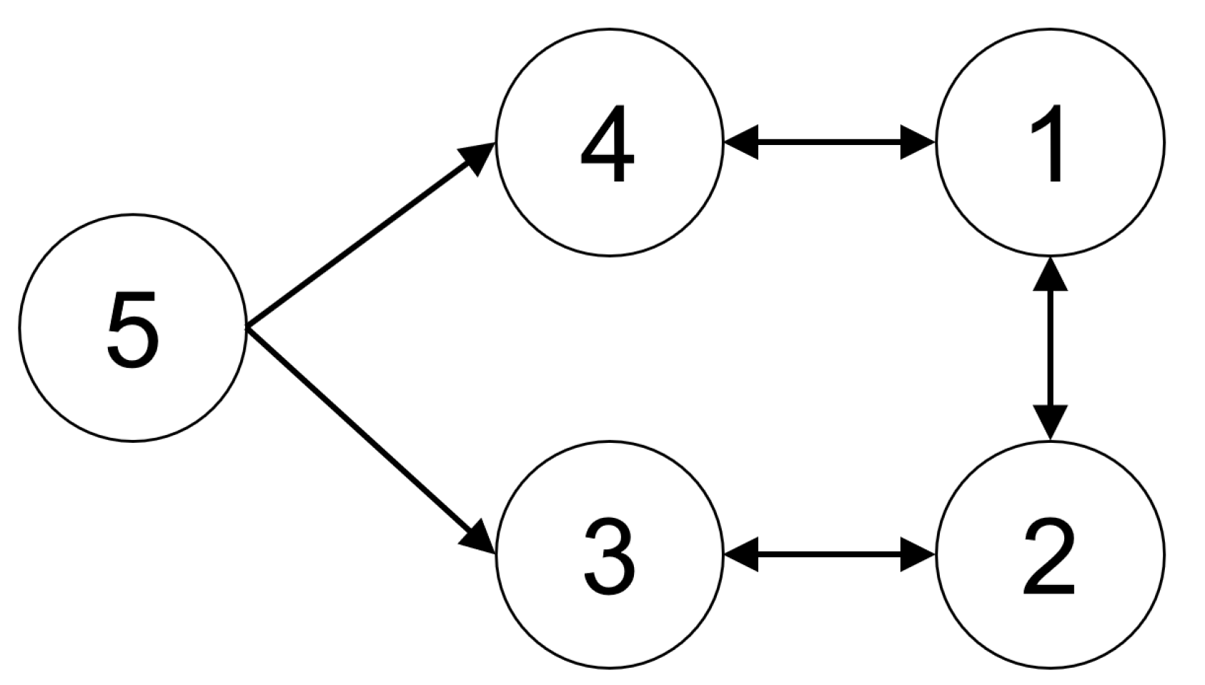
The simulation consisted of a multi-agent system with the network topology illustrated in Figure 1. The system included four follower agents and one leader agent, where agent 5 was designated as the leader.

Each follower agent can obtain information from its respective neighbors, with the neighbor sets defined as follows: $N_1=\{2,4\},N_2=\{1,3\},N_3=\{2,5\},N_4=\{1,5\}$, where $N_i$ is the set of agent i’s neighbors. In contrast, agent 5, as the leader, does not receive information from any other agents. Laplacian matrix L corresponding to this topology is defined as $L=\left[\begin{array}{ccccc}2& -1& 0& -1& 0\\ -1& 2& -1& 0& 0\\ 0& -1& 2& 0& -1\\ -1& 0& 0& 2& -1\\ 0& 0& 0& 0& 0\end{array}\right]$.

The Jordan canonical form of Laplacian matrix L is $\tilde{L}=\left[\begin{array}{cccc}0.382& 0& 0& 0\\ 0& 3.618& 0& 0\\ 0& 0& 1.382& 0\\ 0& 0& 0& 2.618\end{array}\right]$. The corresponding transformation matrices are $\Omega =\left[\begin{array}{ccccc}1& 0.6015& 0.6015& -0.3717& -0.3717\\ 1& 0.6015& -0.6015& 0.3717& -0.3717\\ 1& 0.3717& 0.3717& 0.6015& 0.6015\\ 1& 0.3717& -0.3717& -0.6015& 0.6015\\ 1& 0& 0& 0& 0\end{array}\right]$, and ${\Omega }^{-1}=\left[\begin{array}{ccccc}0& 0& 0& 0& 1\\ 0.6015& 0.6015& 0.3717& 0.3717& -1.9465\\ 0.6015& -0.6015& 0.3717& -0.3717& 0\\ -0.3717& 0.3717& 0.6015& -0.6015& 0\\ -0.3717& -0.3717& 0.6015& 0.6015& -0.4596\end{array}\right]$.

Based on $K\tilde{L}+{\tilde{L}}^{T}K=I$, matrix K is obtained as $\left[\begin{array}{cccc}1.3089& 0& 0& 0\\ 0& 0.1382& 0& 0\\ 0& 0& 0.3618& 0\\ 0& 0& 0& 0.1910\end{array}\right]$. Then, based on related definitions of Lemma 2 and Lemma 3, we can calculate $k={\displaystyle \frac{1}{{\lambda }_{min}\left(K\right)}}=7.2359,{\lambda }_U={\lambda }_{max}\left(U{U}^T\right)=2,{\lambda }_L={\lambda }_{max}\left(L{L}^T\right)=13.0902,{\lambda }_K={\lambda }_{max}\left(K\right)=1.3089,$ and ${\lambda }_{\xi }={\lambda }_{max}\left({(I-J_{n+1})}^T{\xi }^{T}K\xi (I-J_{n+1})\right)=6.3005$.

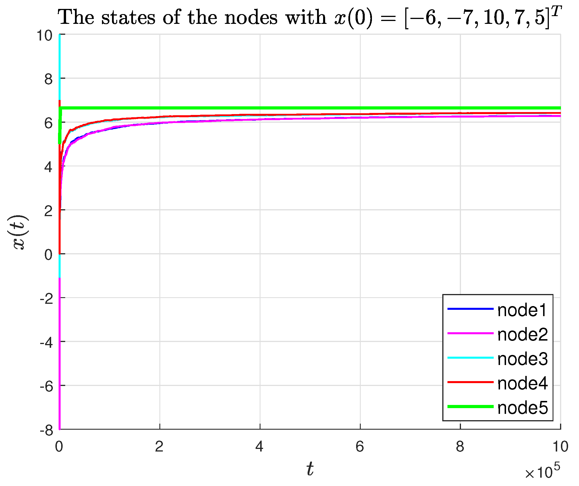
Let the initial values for the states of the agents be $x\left(0\right)={[-6,-7,10,7,5]}^T$, and the initial estimates of the neighbors’ states for each agent be ${[{\hat{x}}_1\left(0\right),{\hat{x}}_2\left(0\right),{\hat{x}}_3\left(0\right),{\hat{x}}_4\left(0\right),{\hat{x}}_5\left(0\right)]}^T={[1,-4,7,2,4]}^T$. The threshold is given as $C=0$, and the state boundary conditions are defined as $W=8$. The noise follows a normal distribution $N(0,8^2)$, and $f_C$ can be computed as $f_C=f\left(\left|C\right|+W\right)=0.0302$.

The state of the leader is convergent, and its state update formula is given by

$$x_5(t+1)=x_5\left(t\right)+g\left(t\right),$$

where $g\left(t\right)={\displaystyle \frac{1}{t^2}}$, which satisfies ${\sum }_{t=1}^{\infty }g\left(t\right)<\infty$. In the simulation, the experimental parameters were set as $\beta =7000$ and $\gamma =4$. The symbol l defined in Theorem 2 can be computed as $l={\displaystyle \frac{{\gamma }^3{\lambda }_U{\lambda }_{L}k}{8{\lambda }_K{\lambda }_{\xi }{d}_{*}}}+{\displaystyle \frac{32{\lambda }_K^3{\lambda }_{\xi }^2{d}_{*}^2}{{\gamma }^3}}+d_{*}$ = 203.0038. 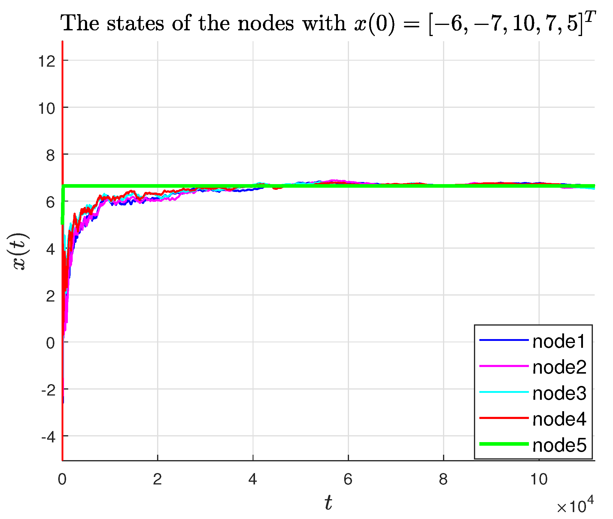Choosing $\beta$ satisfies $\beta >{\displaystyle \frac{l}{f_C}}=6,721.9801$, and the trajectories of the agent states and their estimates are shown in Figure 2 and Figure 3, respectively. 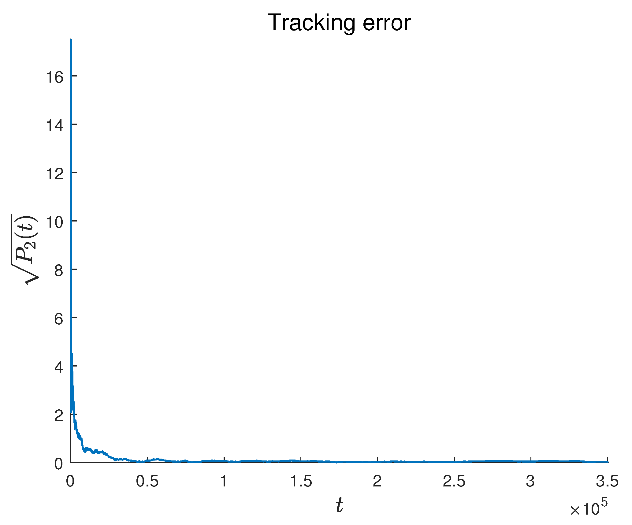Figure 4 and Figure 5 present the tracking error and estimation error, respectively. The results demonstrate that the followers converge to the leader’s state, confirming the theoretical findings in Theorem 1. 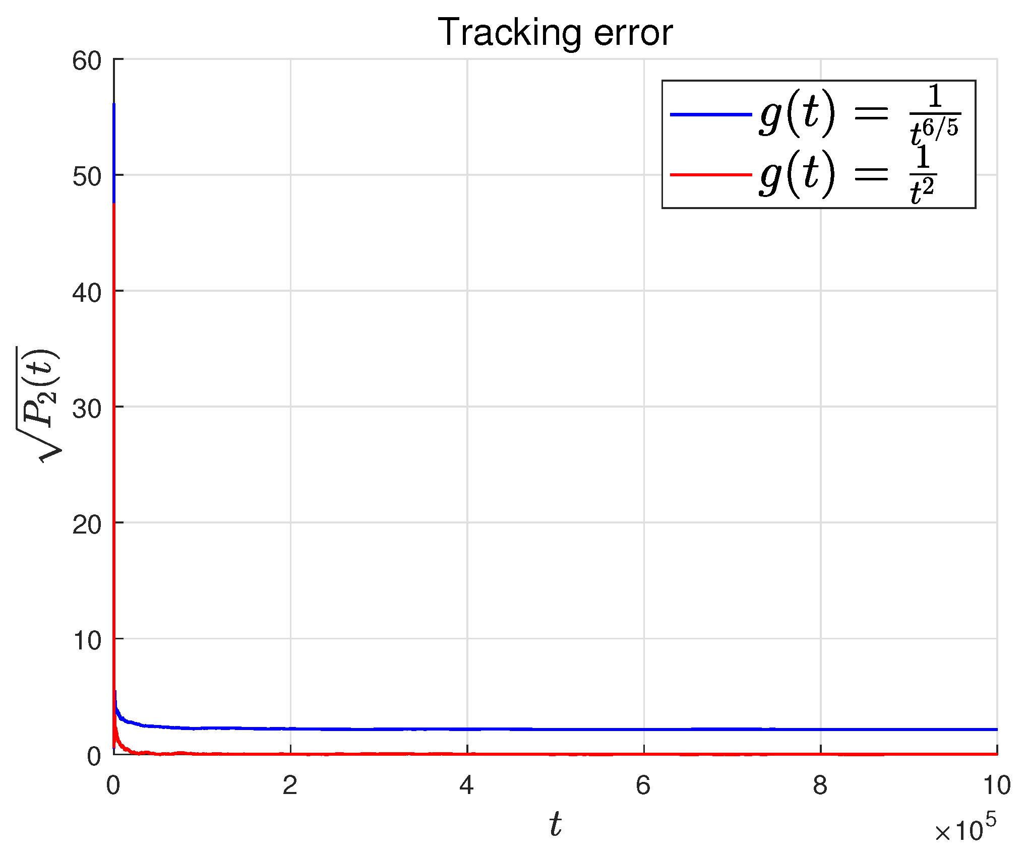Figure 6 shows the relationship between the tracking error and the rate of change of the leader. The faster the leader changes, the slower the tracking error converges, which is consistent with Theorem 2. Figure 7 shows the state–time curves of agents under the P-like algorithm. It can be seen that the convergence to consensus is slower than that of the PD-like algorithm. 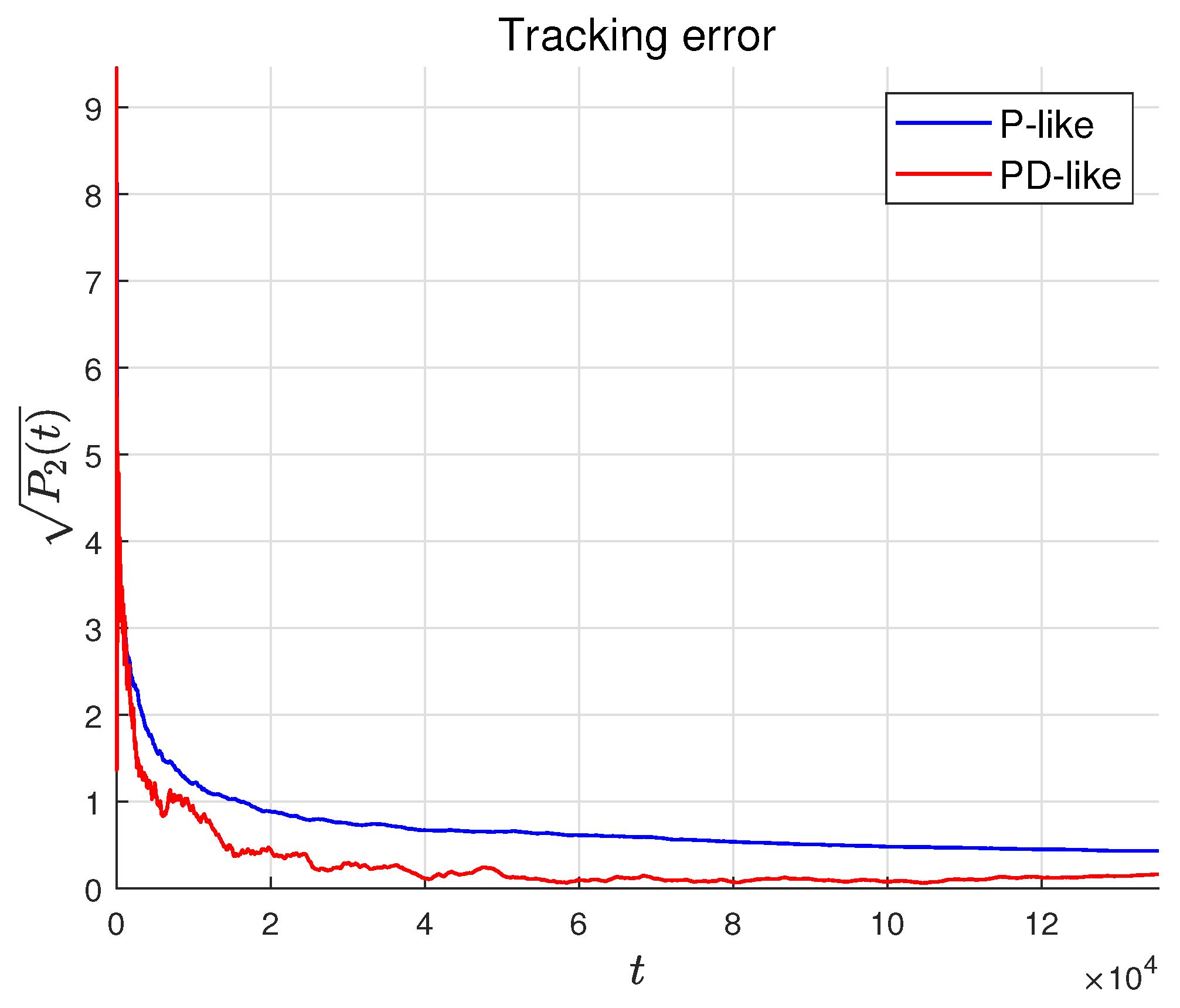At the same time, Figure 8 compares the tracking errors of the two algorithms. The red line represents the PD-like algorithm, and the blue line represents the P-like algorithm. It can also be seen that the PD-like algorithm converges faster.

6. Conclusions

This paper presents a consensus tracking algorithm for discrete-time multi-agent systems under binary-valued communication, considering measurement noise and a time-varying reference state. Each agent estimates the states of its neighbors using RPA and designs a controller to update its state. An estimated differential term is introduced into the controller. Subsequently, the agents can converge to the leader’s reference state, and the convergence speed is closely related to the rate of change of the leader’s state and the system parameters.

There is a lot of work that deserves attention in the future. Presently, the academic community is actively engaged in developing safer and more efficient control algorithms. Notable examples include the design of cooperative control protocols for nonlinear multi-agent systems against different attacks [28,29], and the integration of event-triggered mechanisms into multi-agent consensus tracking problems to significantly reduce system resource consumption while maintaining tracking performance—all of which represent cutting-edge research frontiers [30]. Nevertheless, in practical applications (such as the collective behavior of mobile robots [31]), agents often encounter complex non-matching input constraints, nonlinear dynamic characteristics, and unknown time-varying disturbances. Addressing these challenges by designing robust and adaptive control strategies remains a critical hurdle that demands urgent breakthroughs.