Design and Performance Evaluation of a μ-Synthesis-Based Robust Impedance Controller for Robotic Joints

Abstract

This paper proposes a robust impedance controller to address the performance limitations of mechanical impedance rendering in robotic joints, enabling stable interaction with passive environments. Considering structured uncertainties, such as dynamic parameter perturbations, sensor noise, disturbances, and unmodeled dynamics in actuator models, the $\mathsf{\mu }$-synthesis method is employed to optimize closed-loop robustness performance. This approach minimizes impedance-matching errors in the frequency domain, thereby enhancing the regulation of the systems’s inherent impedance characteristics. Key performance metrics are analyzed, and the impedance-rendering accuracy is evaluated. Furthermore, the limiting factors affecting impedance-matching bandwidth are investigated to inform the selection of impedance parameters and ensure safe physical interaction. The proposed controller is validated through simulations and hardware experiments on a one-DoF modular robotic joint. Frequency domain impedance matching comparisons show that relative to ${\mathcal{H}}_{\infty }$ control, the $\mathsf{\mu }$-synthesis approach reduces impedance matching errors by up to 94.6% and 97.5% under 5% and 30% inertia uncertainties, respectively. Furthermore, experimental results demonstrate that compared to classical impedance control, the proposed method reduces impedance rendering errors by an average of 85.71% across all tested configurations while maintaining superior passivity and interaction stability under diverse impedance conditions. These results validate the effectiveness of $\mathsf{\mu }$-synthesis in achieving safe and high-fidelity physical interaction behavior.

1. Introduction

Mechanical interaction is fundamental to robotic systems, particularly in tasks requiring controlled force and motion [1]. Mechanical interaction dynamics are often characterized by mechanical impedance, and the most common approaches to interaction control regulate either the robot’s impedance or admittance [2]. The goal of impedance control is to achieve a closed-loop behavior that emulates a specified impedance model [3]. Unlike position or force control, where the control goal is to ensure the tracking of the reference input signal (e.g., nominal position or force) [4], impedance control is to match a reference target model that specifies the desired robot-environment interaction, i.e., the relationship between the force and the robot’s motion response. The design of impedance control typically involves two key tasks: the realization and regulation of the desired impedance model. However, achieving accurate impedance rendering under real-world uncertainties (e.g., parameter perturbations, sensor noise, and environmental variations) remains a fundamental challenge.

Impedance control aims to regulate the dynamic interaction between robots and environments by emulating a target impedance model [3]. Traditional approaches fall into two categories, namely dynamic-based and position-based methods. The dynamic-based approach, pioneered by Hogan [3], achieves high-fidelity impedance rendering by compensating for the robot’s intrinsic dynamics [5]. However, its reliance on precise models makes it vulnerable to parameter perturbations and unmodeled dynamics [6]. Conversely, position-based methods enhance robustness through high-gain position tracking, but they often fail to render accurate impedance due to hidden dynamics excited by model errors [5]. Both approaches encounter difficulties when dealing with uncertainties and disturbances, particularly in unstructured environments where stable and accurate impedance control is critical.

To enhance the robustness of impedance control, extensive research has focused on addressing model uncertainties, sensor-actuator non-colocation, and environmental variations. Lawrence [7] compared two control architectures: position-based and torque-based impedance control. The former approach offers ease of implementing rigid behavior but struggles with compliant behavior, while the latter achieves compliance but cannot stably maintain rigidity. These limitations stem from inherent factors such as unmodeled dynamics, sensor-actuator non-colocation, and time delays, which hinder the ability of feedback control to modulate interactive dynamics [8]. For flexible joint robots, the challenge of impedance endering is compounded by increased system order, nonlinearity, and joint flexibility, which degrade performance [4,9].

In response to this, robust control methodologies have been extensively explored. Sliding mode control [10,11], adaptive control [12,13], and ${\mathcal{H}}_{\infty }$ synthesis [14] provide varying levels of robustness against disturbances and parameter variations. Among them, structured robust control via $\mathsf{\mu }$-synthesis [15] has emerged as a promising approach that explicitly models uncertainty sources, including parametric variations, sensor noise, and actuator dynamics, within a unified frequency domain framework. Compared to traditional ${\mathcal{H}}_{\infty }$ design, $\mathsf{\mu }$-synthesis reduces conservatism and enables stricter performance guarantees in impedance matching applications.

Prior research has demonstrated the potential of $\mathsf{\mu }$-synthesis in rigid-body robotic systems. For example, Zhang et al. [16] applied this method to develop compliant force controllers for space docking tasks. Uchimura and Kazerooni [17] proposed a $\mathsf{\mu }$-synthesis-based framework for human–robot collaboration under uncertainty. Aghili [18] extended its application to high-DoF space manipulators interacting with unknown environments. However, these studies largely neglect the structured uncertainties intrinsic to compliant actuation and low-DoF modular joints, where sensor non-collocation, actuator friction, and flexible transmission dominate the interaction behavior.

Recent advances in compliant actuator control have addressed some of these challenges. Fotuhi et al. [19] developed a PID+feedforward (FF) controller for a rotary series elastic actuator (RSEA), incorporating nonlinear friction estimation and model-based compensation. While demonstrating improved performance in trajectory tracking, such methods remain sensitive to unmodeled dynamics and frictional variability, limiting their applicability in uncertain environments. Table 1 summarizes the key characteristics, performance metrics, and limitations of major control methodologies for physical interaction tasks. It highlights the gap between robust stability and accurate impedance rendering in the presence of structured uncertainties.

Table 1. Comparative Analysis of Robust Impedance Control Methods.

Method	Key Characteristics for Robust Stability and Interaction	Limitations and Constraints
Classical PID [20]	Simple to implement; maintains basic stability under nominal conditions. Suitable for rigid environments with low compliance requirements.	Lacks robustness to model uncertainties and sensor noise; poorly handles dynamic or compliant interaction; sensitive to external disturbances.
Adaptive Control [12]	Capable of adjusting to slowly varying system parameters; effective in repetitive tasks with predictable dynamics.	Prone to instability under fast-changing dynamics or impacts; limited in handling high-frequency uncertainties and unmodeled dynamics.
${\mathcal{H}}_{\infty }$ Control [21]	Offers guaranteed robustness to bounded unstructured uncertainties; suitable for worst-case disturbance rejection in mid-frequency range.	Design tends to be overly conservative; ignores structured uncertainties; may restrict achievable impedance shaping bandwidth.
Sliding Mode Control [10]	Highly robust to matched uncertainties and persistent disturbances; effective in maintaining contact force in uncertain environments.	Discontinuous control induces chattering, leading to mechanical wear and unsafe interaction with soft or delicate environments.
Passivity-Based Control [22,23]	Intrinsically stable by enforcing energy dissipation; well-suited for safe interaction with passive or low-stiffness environments.	Cannot handle active or highly dynamic environments; restrictive in rendering high-stiffness or dynamic impedance profiles.
$\mathsf{\mu }$-Synthesis [17,18]	Simultaneously accounts for structured uncertainties (e.g., parametric, sensor, and model uncertainties); enables stable and accurate impedance rendering across a broad stiffness range.	Requires detailed uncertainty modeling and high computational cost for controller synthesis; performance depends on accurate frequency domain characterizations.

Beyond classical stability, interactive robotic systems must ensure coupled stability between the robot and environment dynamics [24]. Passivity theory offers a general framework for ensuring interaction safety [22], but its constraints are overly conservative in high-performance applications [25,26]. High-frequency dynamics and digital implementation issues often break passivity, requiring a relaxation of its strict conditions. To address this, Griggs et al. [27] proposed a hybrid criterion combining passivity at low frequencies with the small-gain theorem at high frequencies. Xia et al. [28] further introduced a passivity index, quantifying how passivity shortages in one system can be compensated by excess passivity in another. These tools have enabled more flexible yet stable designs for high-transparency interaction systems [29]. Our previous study [29,30,31] examined the frequency dependence of impedance and analyzed the accuracy of rendering stiffness in the frequency domain. Furthermore, it was demonstrated that passivity excess in one system can stabilize the interaction when coupled with a system exhibiting passivity shortages, particularly at high frequencies where the system gain is sufficiently small [30,31].

In summary, despite significant advances in robust and passivity-based control, achieving accurate, stable, and transparent impedance rendering under structured uncertainties, particularly in compliant, modular robotic systems, remains a challenging and unresolved issue. To address this, the present study proposes a structured robust impedance control framework based on $\mathsf{\mu }$-synthesis, tailored for low-degree-of-freedom modular robots. The objective is to strike a balance between performance and safety by explicitly modeling multi-source uncertainties, quantifying impedance matching accuracy and passivity degradation, and ensuring coupled stability in the frequency domain.

Accordingly, this study investigates the following research questions: what are the key factors influencing high-fidelity impedance rendering? Can a $\mathsf{\mu }$-synthesis controller achieve robust and passive interaction across varying stiffness and damping configurations? To answer these questions, the proposed control strategy is validated through comprehensive simulations and experiments on a one-DoF modular joint.

The novelties and contributions of this paper include the following:

• A robust impedance control framework leveraging $\mathsf{\mu }$-synthesis to address structured uncertainties in robotic joints, including dynamic parameter perturbations, sensor noise, and actuator dynamics. This framework ensures stable interaction with passive environments while maintaining high-fidelity impedance rendering.
• A novel frequency domain performance index based on the maximum structured singular value ($\mathsf{\mu }$), designed to systematically minimize impedance matching errors and optimize closed-loop robust performance.
• Experimental validation on a modular robotic joint, demonstrating the controller’s effectiveness in achieving accurate impedance rendering and interaction stability under real-world disturbances and uncertainties.

The rest of this article is organized as follows: Section 2 presents the modeling of the robotic system, including the nominal dynamics and structural uncertainties. Section 3 introduces the proposed robust impedance control framework based on $\mathsf{\mu }$-synthesis, along with a detailed methodological formulation. In Section 4, numerical simulations are conducted to examine the effects of key parameters on impedance performance and stability, followed by experimental validation on a one-degree-of-freedom robotic joint and an in-depth analysis of the results. Finally, Section 5 summarizes the main contributions and concludes the paper.

2. Robot Dynamic System Modeling

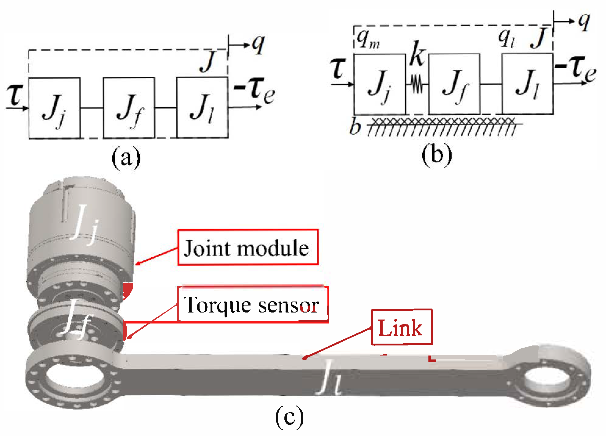
2.1. Dynamic Model

As shown in Figure 1a, under the idealized assumption that the robot joints are rigid, the robot’s rigid dynamic model is

$$\begin{array}{c}J\ddot{q}=\tau -{\tau }_e,\hfill \\ J=J_j+J_f+J_l,\hfill \end{array}$$

(1)

where J is the total inertia, $J_j,J_f,J_l$ represent the inertia of the modular joint side, torque sensor and link side, respectively; q is the absolute position of the link side; $\tau$ and ${\tau }_e$ represent the control input and external torques, respectively.

Figure 1. Joint diagram. (a) Schematic diagram of rigid robot model. (b) Robot joint model with torque sensor dynamics. (c) SolidWorks model of a robot joint module with torque sensor. The nominal parameters are $J_j=0.29\mathrm{kg}·{\mathrm{m}}^2$, $J_f=3.12\times {10}^{-4}\mathrm{kg}·{\mathrm{m}}^2$, $J_l=0.06\mathrm{kg}·{\mathrm{m}}^2$, $k={10}^6\mathrm{Nm}/\mathrm{rad}$, and $b=0.15\mathrm{Nm}/(\mathrm{rad}/\mathrm{s})$.

The rigid-body model in Equation (1) oversimplifies the joint dynamics by neglecting sensor compliance, whereas flexible models explicitly account for stiffness k and damping b to capture energy dissipation and deformation effects. In joints with torque sensors, the non-colocation between the actuator and sensor limits impedance rendering performance. As shown in Figure 1b, considering that $J_f$ is sufficiently small to be negligible, the flexible joint model explicitly considers the torque sensor’s stiffness k and damping b through two degrees of freedom:   

$$\left\{\begin{array}{c}{J}_j{\ddot{q}}_m+b({\dot{q}}_m-{\dot{q}}_l)+k(q_m-q_l)=\tau \hfill \\ J_l{\ddot{q}}_l+b({\dot{q}}_l-{\dot{q}}_m)+k(q_l-q_m)=-{\tau }_e\hfill \end{array}\right.,$$

(2)

where $q_m$ and $q_l$ denote the motor-side and load-side angular positions, respectively. However, the torque sensor’s high stiffness ensures minimal relative displacement within the controller’s operational bandwidth. This allows safe approximation $q_m\approx q_l=q$ for control design while retaining the two-DoF model for impedance rendering performance analysis. Therefore, the simplified dynamical equation of the system motion can be described by

$$\begin{array}{c}J\ddot{q}+b\dot{q}+kq=\tau -{\tau }_e.\hfill \end{array}$$

(3)

Impedance control is typically modeled as a mass-spring-damper system [3], with the objective of rendering the robot’s inherent impedance as the desired impedance [8,9,24]. In the Laplace domain, the desired impedance $Z_d$ is defined as

$$\begin{array}{c}\hfill Z_d\left(s\right)=m_d{\mathrm{s}}^2+b_{d}s+k_d,\end{array}$$

(4)

where $m_d$, $b_d$, and $k_d$ represent the desired mass, damping, and stiffness, respectively. The desired impedance reciprocal is the port admittance $Y_d\left(s\right)={\displaystyle \frac{1}{m_d{s}^2+b_{d}s+k_d}}$. The rendered admittance is $Y_r\left(s\right)=-q/{\tau }_e$, with the rigid model’s inherent port admittance $Y_a^r\left(s\right)={\displaystyle \frac{1}{J{s}^2}}$, and the flexible model’s inherent port admittance $Y_a^s\left(s\right)={\displaystyle \frac{1}{J{s}^2+bs+k}}$.

2.2. Building Uncertain Models

2.2.1. Uncertain Real Parameters

In systems characterized by inherent uncertainties, these uncertainties are typically parameterized by a set of real values. J generally exhibits minimal perturbations, remaining within 1% of its nominal value, even with structural changes or added payloads. k may vary by up to 5%, reflecting material degradation or mechanical property changes under load. b, being the most variable parameter, is assumed to fluctuate by as much as 30%, influenced by factors such as friction, gearbox degradation, and component interactions [30,31]. These assumptions capture the common behavior of robotic systems, thereby improving reliability and adaptability in practical applications.

For the nominal plant model, the inertia parameters were obtained using SolidWorks 2021’ quality properties tool, based on the robot joint components depicted in Figure 1c. The perturbation model includes these uncertainties.

2.2.2. Measurement of Noise Uncertainty

The joint position signal $y_q$ incorporates quantization errors from angle encoder noise ${\eta }_q$, finite resolution artifacts, and pre-amplifier noise. Similarly, the torque measurement $y_{{\tau }_e}$ is contaminated by sensor noise ${\eta }_{{\tau }_e}$. These normalized noise sources are bounded as $\parallel {\eta }_q{\parallel }_{\infty }<1$ and $\parallel {\eta }_{{\tau }_e}{\parallel }_{\infty }<1$ (dimensionless), representing worst-case unit magnitude disturbances. The actual noise characteristics are shaped through frequency-dependent weighting functions:

$$y_q=q+W_{n_q}{\eta }_q,$$

(5)

$$y_{{\tau }_e}={\tau }_e+W_{n_{{\tau }_e}}{\eta }_{{\tau }_e},$$

(6)

where the diagonal uncertainty matrix ${\Delta }_n=\mathrm{diag}({\eta }_q,{\eta }_{{\tau }_e})$ contains normalized noise signals. The weight function is defined as $W_n=\mathrm{diag}(W_{n_q},W_{n_{{\tau }_e}})$, acting as a high-pass filter for noise shaping. The actual noise spectrum can be represented as $W_n{\Delta }_n$.

2.2.3. Input Disturbance

External disturbances, such as force fluctuations during physical interaction or torque ripple from the motor drive, can destabilize the robot’s motion. To systematically account for these effects, we model the input disturbance $u_{d_{\tau }}$ as a filtered uncertainty signal:

$$u_{d_{\tau }}=W_d{\Delta }_{d_{\tau }},$$

(7)

where $W_d$ acts as a filter to simulate these low-frequency disturbances. For the external disturbance $u_{d_{\tau }}$, ${\Delta }_{d_{\tau }}$ represents the effective torque disturbance caused by factors such as motor torque ripple, power amplifier noise, and similar sources.

2.2.4. Actuator Uncertainty

The nominal transfer functions of the actuators are taken as first-order, phase-lag models of

$$G_{an}={\displaystyle \frac{g_d}{T_{d}s+1}},$$

(8)

where $g_d$ and $T_d$ represent the actuator gain and time constant, respectively. This choice provides a simplified yet effective approximation of actuator behavior, especially when the dominant dynamics are governed by low-frequency control bandwidth and when higher-order dynamics (e.g., resonance or structural elasticity) are not explicitly excited within the operational range of interest.

While actuators, in general, can be more accurately represented by second-order models that include inertial and damping effects (e.g., DC motor dynamics or electro-mechanical drives), the first-order approximation is often adopted in impedance control frameworks to emphasize the system’s low-frequency tracking and energy dissipation behavior. Moreover, the assumed first-order structure corresponds to a minimum-phase passive element, which aligns with the passivity constraints often imposed in human–robot interaction systems.

To rigorously account for the higher-order unmodeled dynamics, bandwidth limitations, friction, and actuator nonlinearities, the model incorporates structured input multiplicative uncertainty:

$$G_a\left(s\right)=G_{an}\left(s\right)\left(I+W_a\left(s\right){\Delta }_a\left(s\right)\right),$$

(9)

where $G_a$ is the uncertain actuator model, $W_a$ represents the uncertainty weights of the actuators, and ${\Delta }_a$ captures the uncertain parameters of the actuators, with the norm-bounded uncertainty satisfying $\parallel {\Delta }_a{\parallel }_{\infty }\le 1$.

This formulation ensures that even though the nominal model is simplified to the first order, the robust controller synthesis process accounts for possible higher-order dynamics and performance degradation due to actuator uncertainties. Additionally, the uncertainty weights $W_a\left(s\right)$ are designed based on the empirical step response and frequency response measurements of the physical actuators to conservatively bound the discrepancy from second-order behavior.

3. Methodology

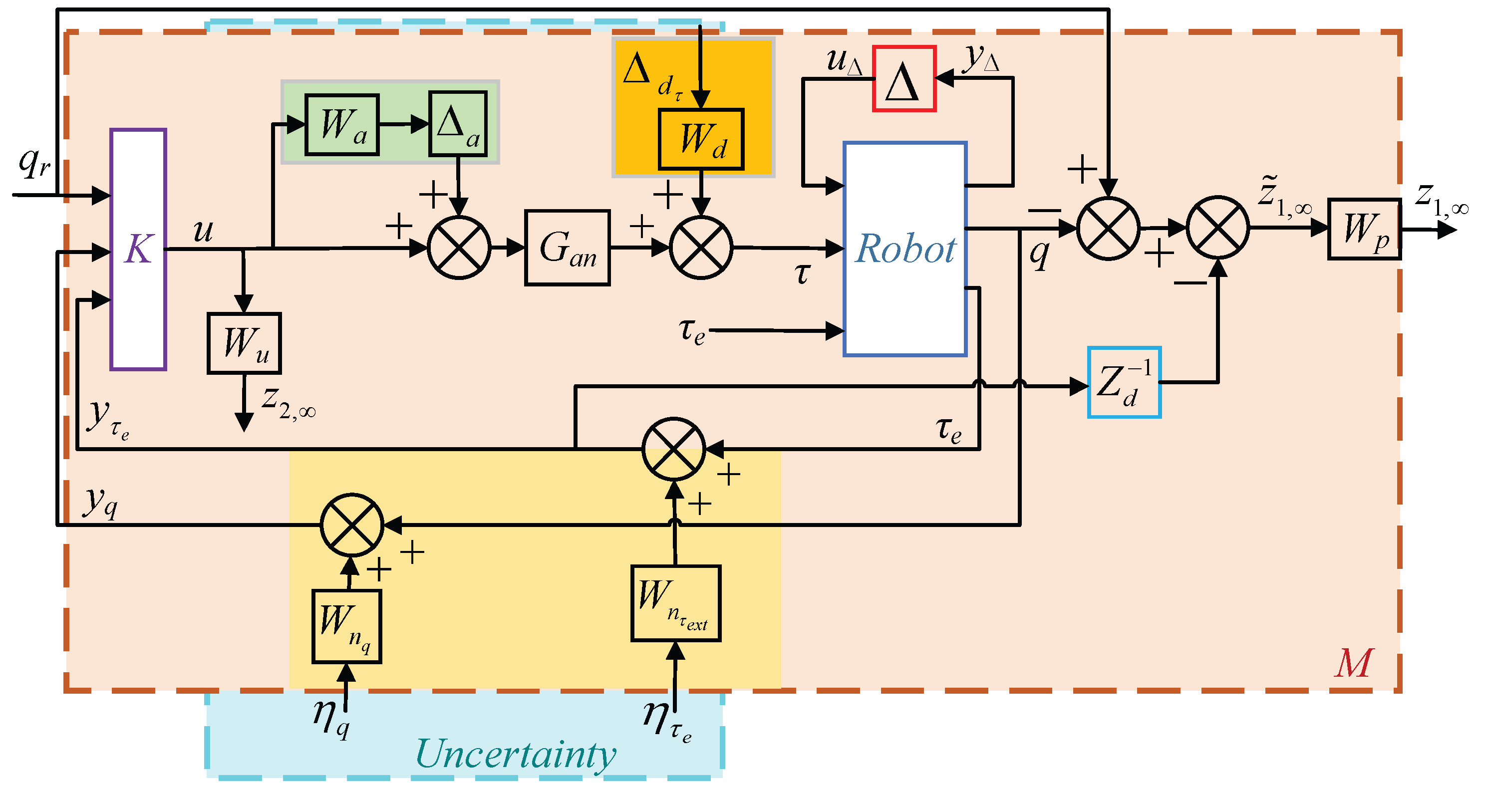
3.1. Robust Impedance Control Framework

All classical controllers (e.g., single-loop, multi-loop, feedforward) can be unified within the generalized $M-\Delta$ framework [14,32]. The closed-loop system is represented as

$$\left[\begin{array}{c}{y}_{\Delta }\\ z\end{array}\right]=\left[\begin{array}{cc}{M}_{11}& M_{12}\\ M_{21}& M_{22}\end{array}\right]\left[\begin{array}{c}{u}_{\Delta }\\ w\end{array}\right],$$

(10)

where M combines the generalized plant P and controller K. This formulation explicitly captures structured and unstructured uncertainties through the $\Delta$ block. $u_{\Delta }$ and $y_{\Delta }$ are the perturbation inputs and outputs, respectively. w denotes the exogenous input typically including command signals, disturbances, noises, etc.; z denotes the error output usually consisting of the regulator output, tracking errors, filtered actuator signals, etc. The signals y and u represent the feedback signals (measured output, tracking error, etc., as the input to the controller) and the control signal (the output from the controller), respectively.

The generalized controlled plant P integrates external disturbances, measurement noise, and actuator saturation to form a comprehensive representation of the system dynamics. $P\left(s\right)$ is partitioned as

$$P=\left[\begin{array}{cc}{P}_{zw}\hfill & P_{zu}\hfill \\ P_{yw}\hfill & P_{yu}\hfill \end{array}\right],$$

(11)

where $P_{zw}\left(s\right)$ is the transfer function from the exogenous input w to the error output z, describing how disturbances affect the performance criteria. $P_{zu}\left(s\right)$ is the transfer function from the control input u to the error output z, illustrating how the control signal influences performance. $P_{yw}\left(s\right)$ represents the transfer function from the exogenous input w to the feedback signal y, indicating how disturbances impact the measurable outputs. $P_{yu}\left(s\right)$ is the transfer function from the control input u to the feedback signal y, showing how the control signal affects the measurable outputs.

In robust control design, one common approach to account for structured uncertainties is to represent the system using a linear fractional transformation (LFT). In our formulation, the uncertain control system is modeled as

$$\left[\begin{array}{c}{y}_{\Delta }\\ z\\ y\end{array}\right]=\left[\begin{array}{ccc}{P}_{11}& P_{12}& P_{13}\\ P_{21}& P_{22}& P_{23}\\ P_{31}& P_{32}& P_{33}\end{array}\right]\left[\begin{array}{c}{u}_{\Delta }\\ w\\ u\end{array}\right].$$

(12)

The structured uncertainty is modeled by

$$u_{\Delta }=\Delta y_{\Delta },$$

(13)

where $\Delta$ is a block-structured operator representing model uncertainties (e.g., parametric variations or unmodeled dynamics) with known bounds. The controller K is implemented through a dynamic output feedback law:

$$u=Ky.$$

(14)

The controller K can be interconnected with the plant P using a LFT. By substituting Equation (14) into Equation (12), the resulting closed-loop system is expressed as follows:

$$\begin{array}{c}M(P,K)=F_l(P,K)\hfill \\ =\left[\begin{array}{cc}{P}_{11}& P_{12}\\ P_{21}& P_{22}\end{array}\right]+\left[\begin{array}{c}{P}_{13}\\ P_{23}\end{array}\right]K{(I-P_{33}K)}^{-1}{\left[\begin{array}{c}{P}_{31}\\ P_{32}\end{array}\right]}^T\hfill \end{array},$$

(15)

where $M\left(s\right)$ is explicitly represented as $M(P,K)$ to indicate that M is constructed from the plant P and the controller K. This integration accounts for both structured and unstructured uncertainties through a LFT framework [14].

The control framework depicted in Figure 2 evaluates performance primarily through impedance matching, which is critical for achieving the desired robot-environment interactions. In this framework, the generalized plant P has two main inputs: disturbance w and control input u, and two outputs: performance metrics z (which includes impedance matching performance $z_{1,\infty }$ and control input constraint $z_{2,\infty }$) and the measurement output y. The external input w is a composite signal comprising the reference trajectory $q_r$, position measurement $y_q$, and external force-related measurement $y_{{\tau }_e}$. The design objective is to tune the performance weighting function $W_p$ to minimize these performance metrics, which is defined as follows:

$$\begin{array}{c}\hfill z_{1,\infty }=\left\{\begin{array}{c}{W}_p\left(q_r-q-{\displaystyle \frac{{\tau }_e}{Z_d}}\right),{\tau }_e\ne 0,\\ W_p(q_r-q),{\tau }_e=0.\end{array}\right.\end{array}$$

(16)

Figure 2. Block diagram of the closed-loop robotic system for impedance matching control. The generalized plant P interacts with the controller K via feedback loops based on sensor measurements and control outputs. The feedback paths include joint position $y_q$ and external force-related measurements $y_{{\tau }_e}$, which are influenced by measurement noise (yellow blocks, e.g., $W_{n_q}$, $W_{n_{{\tau }_e}}$). The control input u passes through actuator dynamics (orange blocks, e.g., $G_{an}$) and actuator uncertainty (e.g., $W_a$, ${\Delta }_a$) before acting on the robot. Disturbance paths from motor ripple and environmental disturbances are captured by green blocks (e.g., $W_d$, ${\Delta }_{d_{\tau }}$), which directly affect the torque output $\tau$ and hence the interaction force. The regulated outputs $z_{1,\infty }$ and $z_{2,\infty }$ quantify impedance matching accuracy and control effort, respectively. This diagram highlights the full flow of data, disturbances, and feedback signals critical to evaluating system robustness and performance.

3.2. $\mu$-Synthesis Problem

A dynamic output feedback control law $u=K\left(s\right)y$ is designed to achieve impedance matching, robust stability, and interaction stability. The closed-loop transfer function from disturbance w to performance output z, denoted as $T_{w\to z}\left(K\right)$, quantifies the system’s ability to attenuate disturbances while maintaining stability. The state-space representation of $K\left(s\right)$ is given by

$$\begin{array}{c}\dot{\zeta }=A_K\zeta +B_{K}y\hfill \\ u=C_K\zeta +D_{K}y\hfill \end{array},$$

(17)

where $\zeta \in {\mathbb{R}}^n$ is the controller’s internal state vector (n: controller order); $A_K\in {\mathbb{R}}^{n\times n}$ governs the controller’s internal dynamics; $B_K\in {\mathbb{R}}^{n\times m}$ maps the measured outputs y (dimension m) to state updates; $C_K\in {\mathbb{R}}^{p\times n}$ generates the control input u (dimension p) from the states; and $D_K\in {\mathbb{R}}^{p\times m}$ provides direct feedforward from measurements to the control input. The system incorporating K achieves robust performance if and only if ${\mu }_{\Delta }\left(T_{zw}\left(j\omega \right)\right)<1$, which is equivalent to the condition ${∥T_{w\to z}\left(K\right)∥}_{\infty }<1$. The controller’s state-space representation follows the standard dynamic output feedback architecture, where the state derivative $\dot{\zeta }$ depends on both the controller’s internal dynamics ($A_K\zeta$) and the measured output y ($B_{K}y$). This enables real-time adaptation to system uncertainties and disturbances while maintaining closed-loop stability. These  matrices are computed via the D-K iteration to minimize the peak value of the structured singular value ${\mu }_{\Delta }$, ensuring robust stability and performance.

The objective of $\mathsf{\mu }$-synthesis is to minimize the peak value of the structured singular value ${\mu }_{\Delta }\left(·\right)$ of the closed−loop transfer function matrix $F_l(P,K)$ over the set of all stabilizing controllers K. This can be formally expressed as

$$\underset{K\mathrm{stabilizing}}{min}\underset{\omega }{max}{\mu }_{\Delta }\left(F_l(P,K)\left(j\omega \right)\right),$$

(18)

where ${\mu }_{\Delta }\left(M\right)$ quantifies the smallest structured perturbation $\Delta$ (normalized to ${\parallel \Delta \parallel }_{\infty }\le 1$) that destabilizes the closed−loop system or violates performance specifications. Here, $\Delta$ represents the structured uncertainties, including parametric variations (e.g., inertia ${\Delta }_J$, damping ${\Delta }_b$), sensor noise ${\Delta }_n$, and actuator dynamics ${\Delta }_a$. Stability is guaranteed if the structured singular value ${\mu }_{\Delta }\left(M\left(j\omega \right)\right)<1$ for all $\omega$, where M is the closed−loop transfer matrix and $\Delta =\mathrm{diag}({\Delta }_{\mathrm{struct}},{\Delta }_{\mathrm{unstruct}})$.

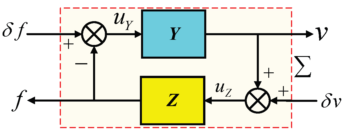
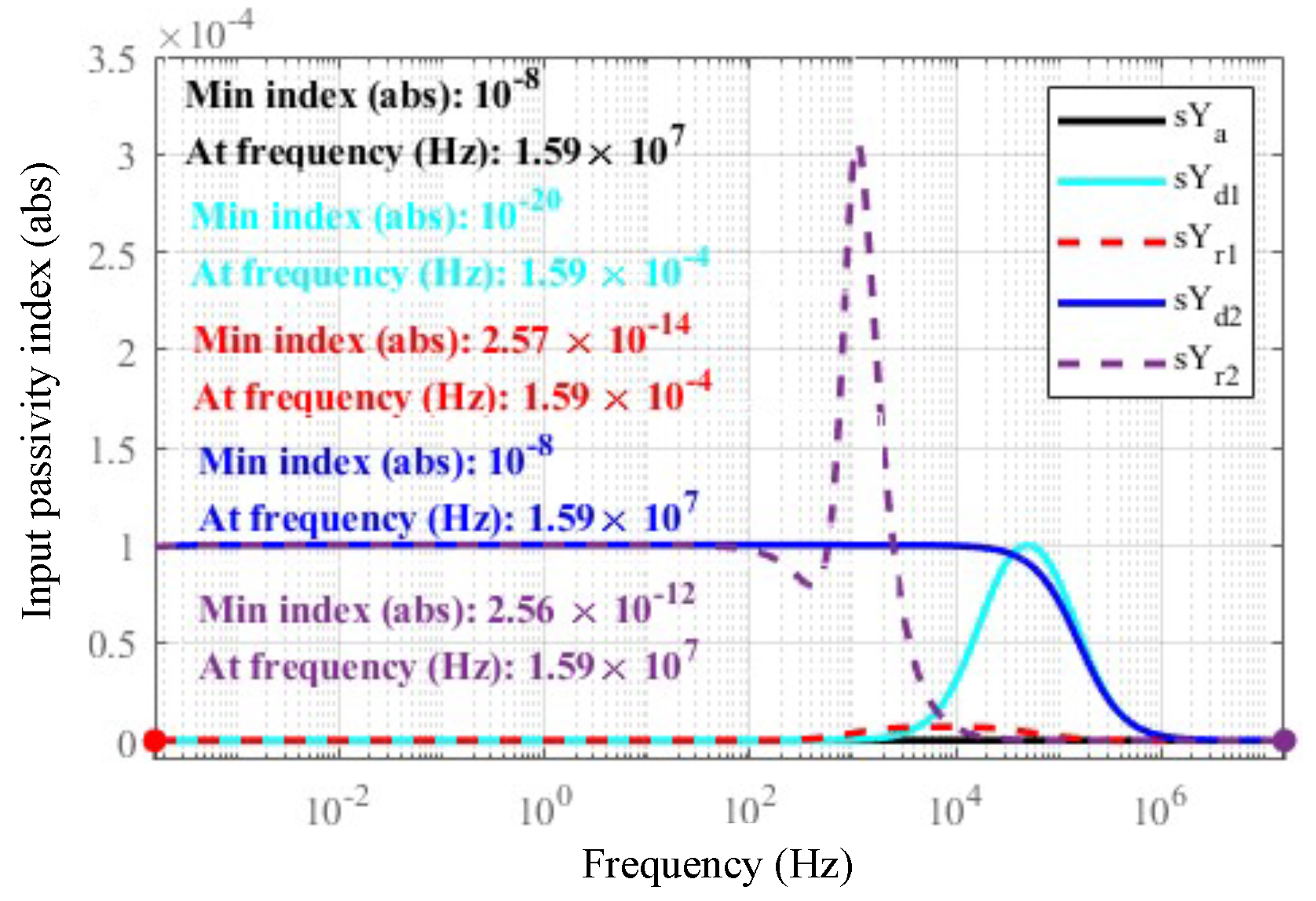
3.3. Interaction Stability Based on Passivity Index

Interaction stability refers to a system’s ability to maintain stable behavior during dynamic interactions between the robot and the environment [33]. Consider a system $G\left(s\right)$ with input u and output y. The system is passive if there exists a constant $\beta \le 0$ such that:

$${⟨u,y⟩}_T\ge \beta ,\forall T\ge 0,$$

(19)

where T denotes the time interval over which the energy inner product ${⟨u,y⟩}_T$ is defined as

$${⟨u,y⟩}_T={\int }_0^{T}u{\left(t\right)}^{\top }y\left(t\right)dt.$$

(20)

For the 1-DoF robotic joint interacting with the environment, the input-output pair $(u,y)$ corresponds to the interaction port $({\tau }_e,\dot{q})$, where:

• ${\tau }_e$ (input u) is the external torque (unit: Nm),
• $\dot{q}$ (output y) is the angular velocity (unit: rad/s).

Since both u and y are scalars in this case ($u,y\in {\mathbb{R}}^1$), the inner product ${⟨u,y⟩}_T$ is well defined and represents the mechanical work exchanged between the robot and environment over time T.

If there are constants $\rho$ and v such that

$${⟨u,y⟩}_T\ge \beta +\rho {⟨y,y⟩}_T+v{⟨u,u⟩}_T,$$

(21)

then, the system exhibits input-feedforward-output-feedback passivity (IF-OFP(v,$\rho$)) [28].

The input feedforward passivity (IFP) index v is defined as

$$v\left(G\left(s\right)\right)=0.5\underset{\omega }{min}{\lambda }_{min}\left(G\left(j\omega \right)+G^H\left(j\omega \right)\right),$$

(22)

where $G\left(s\right)$ is the system transfer function, $G^H$ denotes its conjugate transpose, and ${\lambda }_{min}$ is the smallest eigenvalue. A positive v implies energy dissipation at the input port.

The output passivity index is defined as

$$\rho \left(G\left(s\right)\right)=0.5\underset{\omega }{min}{\lambda }_{min}\left(G^{-1}\left(j\omega \right)+G^{-H}\left(j\omega \right)\right).$$

(23)

A positive $\rho$ ensures energy dissipation at the output port, critical for stabilizing passive environments.

The interaction model between the robot’s admittance Y and the environment’s impedance Z forms a negative feedback loop, as shown in Figure 3. The robot admittance $Y\left(s\right)$ receives the external torque input $u_Y=-{\tau }_e+{\delta }_f$ and outputs the angular velocity $v=\dot{q}$, while the environment impedance $Z\left(s\right)$ receives the velocity input $u_Z=\dot{q}+{\delta }_v$ and outputs the interaction force $f={\tau }_e$. The perturbations ${\delta }_v$ and ${\delta }_f$ represent velocity and force disturbances caused by sensor noise, unmodeled dynamics, or environmental uncertainties. This interconnection ensures that the passivity indices of $Y\left(s\right)$ and $Z\left(s\right)$ compensate for energy losses or gains through ${\delta }_v$ and ${\delta }_f$. The overall system passivity and stability are governed by the properties of Y and Z. If constants ${\delta }_Y$ and ${\epsilon }_Z$ satisfy ${\delta }_Y+{\epsilon }_Z\ge 0$, with Z having OFP(${\epsilon }_Z$) and Y having IFP(${\delta }_Y$), then the system $\Sigma$ is passive if ${\delta }_Y+{\epsilon }_Z=0$ and ${\mathcal{L}}_2$-stable when ${\delta }_Y+{\epsilon }_Z>0$.

Figure 3. Negative feedback interconnection between the robot’s admittance $Y\left(s\right)$ and the environment’s impedance $Z\left(s\right)$.

One system, either Z or Y, may exhibit non-passivity as long as the other compensates with excess passivity [28]. Furthermore, interaction stability remains robust to uncertainties if ${\delta }_Y+{\epsilon }_Z>0$ [30].

3.4. Impedance Control $\mu$-Synthesis via D-K Iteration

To achieve robust impedance control under structured uncertainties, the $\mathsf{\mu }$-synthesis method is employed. This approach iteratively minimizes the structured singular value ${\mu }_{\Delta }$ of the closed-loop transfer matrix by alternating between two main steps, namely the D-step and the K-step [34]. Through $\mathsf{\mu }$-synthesis, an N-order controller is designed, reducing the peak value of $\mathsf{\mu }$ to less than 1, achieving robust stability and performance in the closed-loop system. This process can be expressed as

$$\underset{K}{min}\left(\underset{D\left(j\omega \right)}{min}{∥D\left(j\omega \right)M\left(K\left(j\omega \right)\right)D^{-1}\left(j\omega \right)∥}_{\infty }\right).$$

(24)

The D-K iteration process comprises four fundamental stages executed sequentially:

Initialization: Start with an initial controller $K_0\left(s\right)$ or identity controller.

D-step: For a fixed controller $K_i\left(s\right)$, compute the frequency-dependent scaling matrices $D\left(j\omega \right)$ and $D^{-1}\left(j\omega \right)$ that minimize an upper bound of ${\mu }_{\Delta }$:

$${\mu }_{\Delta }\left(M\left(K_i\left(j\omega \right)\right)\right)\approx {\parallel D\left(j\omega \right)M\left(K_i\left(j\omega \right)\right)D^{-1}\left(j\omega \right)\parallel }_{\infty }.$$

(25)

K-step: Using the computed scaling $D\left(j\omega \right)$, solve an ${\mathcal{H}}_{\infty }$ optimization problem to update the controller:

$$K_{i+1}\left(s\right)=arg\underset{K}{min}{\parallel D\left(j\omega \right)M\left(K\left(j\omega \right)\right)D^{-1}\left(j\omega \right)\parallel }_{\infty }.$$

(26)

Convergence: Repeat steps 2–3 until ${\mu }_{\Delta }<1$ is achieved over the desired frequency range.

The final controller $K^{*}\left(s\right)$ guarantees robust stability and performance for all admissible uncertainties. This synthesis approach ensures the system tolerates sensor noise, actuator imperfections, and environmental variations while achieving desired impedance rendering fidelity.

3.5. Weighting Functions Selection

The selection of weighting functions require iterative tuning, as no universal method that applies to all cases [14]. The goal is to design weighting functions that capture the unique characteristics of disturbances and noise sources, such as sensor noise, interference, and actuator uncertainty, which can affect system stability and performance. For example, $W_{n_q}=2\times {10}^{-5}{\displaystyle \frac{10s+1}{0.1s+1}}$ and $W_{n_{{\tau }_e}}=6\times {10}^{-4}{\displaystyle \frac{0.1s+1}{0.001s+1}}$ act as high-pass filters for frequencies above 500 Hz. $W_d$, for the range [0.001, 10] Hz, is defined as $W_d={\displaystyle \frac{1}{0.0005s+1}}$. Actuator uncertainty is modeled by $W_a={\displaystyle \frac{0.3877s+25.6011}{s+246.3606}}$, while $W_u=10{\displaystyle \frac{s+10}{s+1000}}$ penalizes high−frequency components to prevent actuator saturation.

The performance weighting function $W_p$, designed as a low−pass filter, is crucial for balancing impedance matching accuracy (IMA), impedance matching bandwidth (IMB), tracking performance, robustness, and interaction stability. Impedance rendering performance is assessed by normalizing the rendered impedance $Z_r\left(j\omega \right)$ to the desired impedance $Z_d\left(j\omega \right)$, with IMA quantified as $\mathrm{IMA}=G_{\mathrm{peak}}-1$, where $G_{\mathrm{peak}}$ represents the worst−case peak gain over the relevant frequencies. For MIMO systems, $G_{\mathrm{peak}}$ corresponds to the largest singular value of the frequency response matrix. To minimize IMA, $W_p$ is iteratively refined based on the computed error. Using MATLAB’s wcgain function, the worst−case gain (${\mathcal{H}}_{\infty }$-norm) is estimated, offering an upper bound while considering system uncertainties [35]. This ensures IMA is controlled within acceptable limits without compromising system stability.

3.6. Performance Metrics and Iterative Tuning

To systematically evaluate and improve the performance of the impedance controller synthesized via D-K iteration, admittance−based performance metrics are introduced. The impedance rendering accuracy is quantified by IMA, which is defined as the ${\mathcal{H}}_{\infty }$ norm of the normalized impedance tracking error:

$$\mathrm{IMA}={∥{\displaystyle \frac{Y_r\left(s\right)-Y_d\left(s\right)}{Y_d\left(s\right)}}∥}_{\infty }.$$

(27)

This metric reflects the worst−case gain deviation between the achieved and desired impedance over the frequency domain and provides a conservative bound on system fidelity in interaction−dominant tasks.

In parallel, the bandwidth over which accurate impedance rendering is maintained is captured by IMB, defined as the frequency range where the magnitude ratio satisfies the 3 dB threshold:

$$\left|{\displaystyle \frac{Y_r\left(j\omega \right)}{Y_d\left(j\omega \right)}}\right|\le \sqrt{2}.$$

(28)

This definition ensures that within the IMB range, the rendered mechanical impedance follows the target profile closely enough for practical interactive performance, such as stable physical contact and precise force tracking.

The iterative tuning of the performance weighting function $W_p\left(s\right)$ is guided by these metrics. For instance, increasing the low−frequency gain of $W_p\left(s\right)$ allows the controller to track low−frequency components more accurately, thereby improving IMA. Conversely, enhancing  the high-frequency roll−off of $W_p\left(s\right)$ helps maintain robustness by avoiding the amplification of sensor noise or model uncertainties.

Each iteration of controller synthesis involves updating $W_p\left(s\right)$, recomputing the structured singular value ${\mu }_{\Delta }$, and performing D-K iteration to synthesize a new robust controller. Structured singular value analysis provides a rigorous means to verify whether the closed−loop system satisfies robust stability and robust performance under parametric and dynamic uncertainties. The upper bound of ${\mu }_{\Delta }$ across all frequencies is monitored to ensure it remains below unity, which confirms that the system maintains desired performance while tolerating modeling errors, external disturbances, and actuator variations. This closed−loop iteration continues until both the impedance/admittance tracking metrics and the robustness margins converge to satisfactory levels.

4. Results and Discussion

4.1. Simulation Setup

The simulation was carried out on a computer equipped with a 12th Generation Intel^® Core™ i7-12700F processor (8 cores, 16 threads, 25 MB cache, 2.1 GHz base frequency, 4.9 GHz turbo frequency). The control framework and all relevant simulation models were developed within the MATLAB 2021b/Simulink environment, leveraging the Robust Control Toolbox to validate the performance and robustness of the proposed $\mathsf{\mu }$-synthesis-based impedance controller. The simulation parameters were carefully selected to reflect realistic mechanical and control system conditions, as summarized in Table 2.

Table 2. Model parameters and uncertainty ranges used in simulations.

Parameter	Symbol	Nominal Value	Uncertainty/Notes
Joint inertia	$J_j$	0.29	$\pm 5\%$
Torque sensor inertia	$J_f$	$3.12\times {10}^{-4}$	$\pm 5\%$
Link inertia	$J_l$	0.06	$\pm 5\%$
Joint stiffness	k	${10}^6$	$\pm 5\%$
Joint damping	b	$0.15$	$\pm 30\%$
Actuator gain	$g_d$	1.0	Fixed
Actuator time constant	$T_d$	0.01	First-order lag
Position noise weighting function	$W_{n_q}\left(s\right)$	$2\times {10}^{-5}·{\displaystyle \frac{10s+1}{0.1s+1}}$	Noise model for position measurement
Torque noise weighting function	$W_{n_{{\tau }_e}}\left(s\right)$	$6\times {10}^{-4}·{\displaystyle \frac{0.1s+1}{0.001s+1}}$	Noise model for torque measurement
External disturbance weighting function	$W_d\left(s\right)$	${\displaystyle \frac{1}{0.0005s+1}}$	Disturbance input

To ensure robustness under these uncertainties, the control design was formulated using LFT techniques. The generalized plant $P\left(s\right)$ was assembled using the connect and sysic functions in MATLAB 2021b, capturing all performance, uncertainty, and noise channels. The controller synthesis was performed using the musyn function, which executes the D-K iteration procedure to minimize the structured singular value $\mathsf{\mu }$. Post-synthesis validation was carried out using the wcgain function to assess worst-case closed-loop gain under all permissible perturbations.

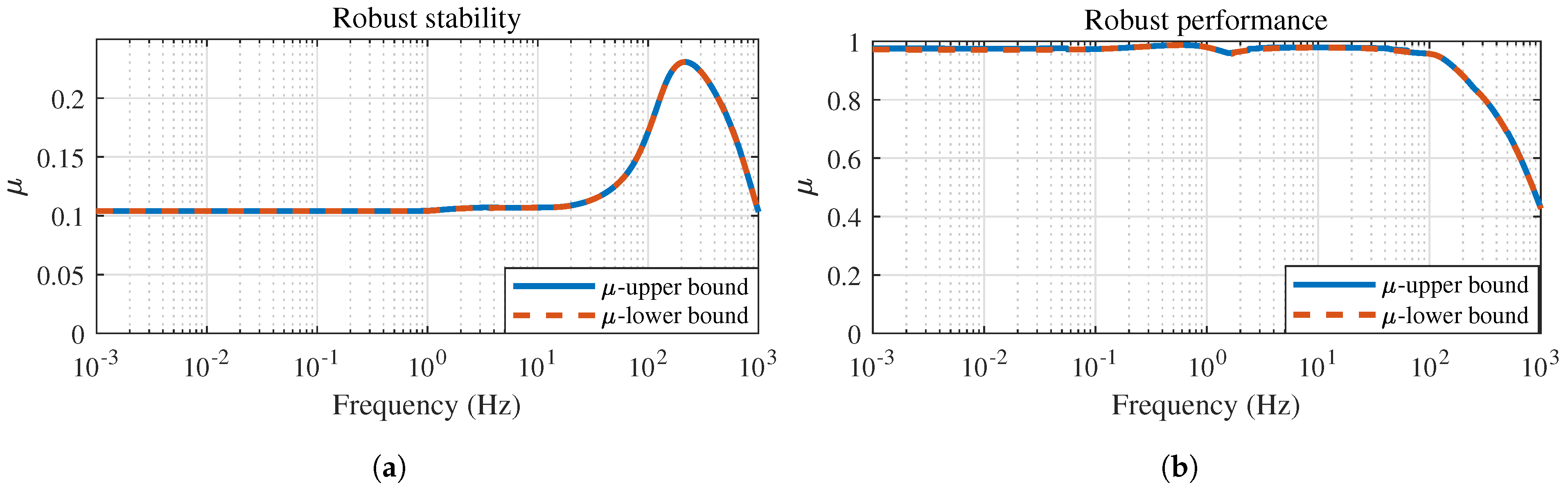
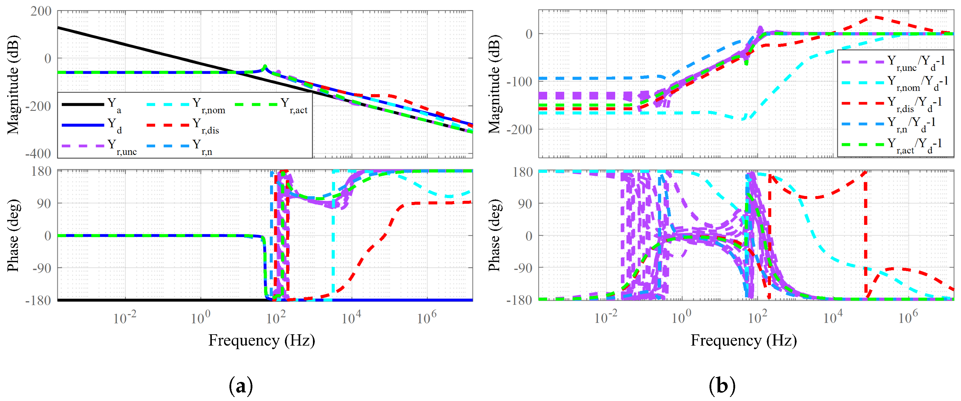
4.2. Robust Stability and Performance Assessment of the Closed-Loop System

To evaluate the robustness of the proposed impedance controller against structured model uncertainty, we conducted both robust stability and robust performance analyses based on the structured singular value (SSV) framework. Specifically, the robuststab function was utilized to assess the robust stability margins of the closed−loop system, without requiring a specific M – $\Delta$ form. This method computes upper and lower bounds of $\mathsf{\mu }$ across the frequency spectrum, and the corresponding stability margins are given by $\mathrm{LowerBound}=1/{\beta }_u$ and $\mathrm{UpperBound}=1/{\beta }_l$, where ${\beta }_u$ and ${\beta }_l$ are the frequency−wise maxima of the upper and lower bounds of $\mathsf{\mu }$, respectively.

As shown in Figure 4a, the computed upper and lower bounds of $\mathsf{\mu }$ remain strictly below one over the entire frequency range, indicating that the closed−loop system maintains robust stability for all modeled perturbations. The detailed results show that the system tolerates up to 427% of the modeled uncertainty (stability margin $>4.27$), with a destabilizing perturbation occurring at approximately 224.57 rad/s. Furthermore, the eigenvalues of the controller, listed in the simulation log, all lie in the left−half complex plane, confirming nominal internal stability.

Figure 4. Robustness analysis of the controller under the desired impedance parameters: $k_d=1000\mathrm{Nm}/\mathrm{rad}$, $b_d=0.1\mathrm{Nm}/(\mathrm{rad}/\mathrm{s})$, and $m_d=0.01{\mathrm{kg}\text{·}\mathrm{m}}^2$. (a) The robust stability of the controller. (b) The robust performance of the controller.

The robust performance is further assessed using the robustperf function, which evaluates whether the system remains stable and meets performance specifications under extended uncertainty ${\Delta }_P$. The D−K iteration converges within eight steps to a best achieved $\mathsf{\mu }$ peak value of 0.951, as summarized in the iteration table. As shown in Figure 4b, the frequency−dependent bounds of $\mathsf{\mu }$ are also strictly less than one. This indicates that the system not only preserves robust stability but also satisfies the weighted performance requirement ${∥T_{w\to z}\left(s\right)∥}_{\infty }<1$ under all admissible uncertainties. Consequently, both robust stability and robust performance are guaranteed for the desired impedance parameters $k_d=1000$ Nm/rad, $b_d=0.1$ Nm/(rad/s), and $m_d=0.01$ kg $·$ ${\mathrm{m}}^2$.

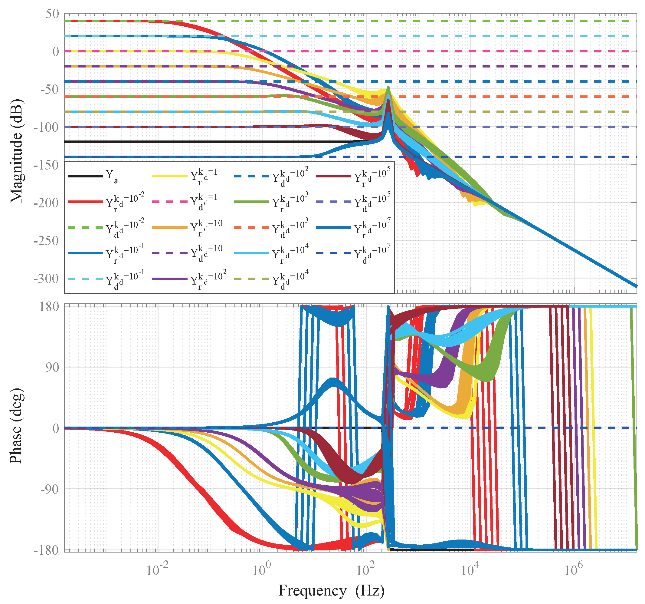
4.3. Evaluation of Impedance Rendering Performance

To systematically evaluate the controller’s sensitivity to key impedance parameters, we conducted a comprehensive parametric study examining the effects of desired stiffness ($k_d$), damping ($b_d$), and inertia ($m_d$) on the system’s rendering performance.

When rendering a pure virtual spring with stiffness $k_d$, the cutoff frequency (CF), $f_c$, is given by $f_c={\displaystyle \frac{1}{2\pi }}\sqrt{{\displaystyle \frac{k_d}{J}}}$, which provides an estimate of the upper bound of the impedance rendering performance. The frequency domain impedance matching results are shown in Figure 5. The uncontrolled admittance, $Y_a$, represents the inherent system behavior, whereas the rendered admittance $Y_r$ closely approximates $Y_d$ within the frequency domain region of interest.

Figure 5. Puredesired stiffness $k_d$ rendering performance.

The approximation of the rendered impedance to the desired impedance shows increased uncertainty near the system’s resonant frequency. This uncertainty is also evident in Figure 6a,b. The system demonstrates strong stiffness rendering fidelity in low−frequency regimes, with near-perfect tracking of desired $k_d$ values below the cutoff frequency. However, this sensitivity diminishes sharply as frequency approaches the system’s natural resonance, where small variations in commanded stiffness can cause disproportionate changes in rendered impedance. The stiffness rendering accuracy recovers partially at supra-resonant frequencies, though it is ultimately limited by the physical plant dynamics.

Figure 6. Impedance rendering performance. (a) Different values of $b_d$ with $k_d=10\mathrm{Nm}/\mathrm{rad}$. (b) Different values of $m_d$ with $k_d=1000\mathrm{Nm}/\mathrm{rad}$ and $b_d=0.1\mathrm{Nm}/(\mathrm{rad}/\mathrm{s})$.

Table 3 quantitatively characterizes stiffness-dependent control performance across nine orders of magnitude. The robust closed-loop stability margin (RCSM > 1.12 in all cases) confirms unconditional stability within modeled uncertainties, peaking at 2.59 for $k_d={10}^3$ Nm/rad, where controller dynamics optimally balance performance robustness tradeoffs. Settling time (ST) exhibits a bimodal distribution—decreasing from 21.43 s to 2.43 s as $k_d$ increases from ${10}^{-2}$ to 10 Nm/rad, then temporarily rising to 9.05 s at $k_d={10}^3$ Nm/rad due to second-order resonance effects before stabilizing near 2 s. Closed-loop bandwidth (CLB) demonstrates logarithmic correlation with $k_d$, expanding from 0.035 Hz to 865.2 Hz while maintaining overshoot (OS) below 18.21%. The weighting function $W_p\left(s\right)$ structurally evolves with stiffness: low $k_d$ (<10 Nm/rad) utilizes first-order filters with integral action, transitioning to second-order forms at higher stiffness to manage resonant modes.

Table 3. Performance specification results.

${\mathit{k}}_{\mathit{d}}$ (Nm/rad)	${\mathit{W}}_{\mathit{p}}\left(\mathit{s}\right)$	CF (Hz)	IMA	IMB (Hz)	ST (s)	OS (%)	CLB (Hz)	RCSM
${10}^{-2}$	${\displaystyle \frac{{10}^{-5}s+0.01}{s+{10}^{-5}}}$	0.027	0.089	0.024	21.43	12.52	0.035	1.52
${10}^{-1}$	${\displaystyle \frac{{10}^{-5}s+0.1}{s+0.0002}}$	0.086	0.013	0.157	15.72	18.21	0.112	1.58
1	${\displaystyle \frac{{10}^{-5}s+2}{s+0.0002}}$	0.272	0.006	0.252	5.89	5.13	0.327	1.81
${10}^1$	${\displaystyle \frac{{10}^{-5}s+10}{s+0.001}}$	0.861	0.003	0.511	2.43	2.75	0.854	1.75
${10}^2$	${\displaystyle \frac{{10}^{-5}s+50}{s+0.005}}$	2.722	0.002	1.127	3.21	1.33	2.141	2.05
${10}^3$	${\displaystyle \frac{{10}^4}{0.5s^2+1.2s+1}}$	8.607	0.004	7.615	9.05	1.86	8.912	2.59
${10}^4$	${\displaystyle \frac{{10}^4}{0.05s^2+1.2s+1}}$	27.22	0.007	13.78	2.04	0.23	28.37	1.12
${10}^5$	${\displaystyle \frac{{10}^5}{0.05s^2+0.1s+1}}$	86.07	0.008	37.27	2.02	0.10	89.45	1.47
${10}^7$	${\displaystyle \frac{{10}^5}{0.005s^2+0.45s+1}}$	860.7	0.032	859.0	2.01	0.62	865.2	1.43

To further investigate the sensitivity of the controller to key impedance parameters, a parametric study was conducted on the desired damping $b_d$ and desired inertia $m_d$. Figure 6a illustrates that increasing $b_d$ enhances damping matching across a broader low−frequency range, whereas a smaller $b_d$ causes the low−frequency $k_d$ characteristics to dominate, hindering the rendering of $b_d$. This sensitivity recovers partially at supra−resonant frequencies, though it is constrained by the physical actuator limitations evident in the high−frequency roll−off characteristics.

Figure 6b depicts the rendering of $k_d$ at low−frequency and $b_d$ at mid−frequency. At high frequencies, $m_d$ dominates the impedance characteristics; however, the “waterbed effect” limits the system’s ability to render small values of $m_d$. Increasing $m_d$ improves the system’s capability to render it across low− and mid−frequency, enabling effective impedance behavior below the cutoff frequency. Nevertheless, achieving low virtual mass impedance at high frequencies remains inherently difficult in practice. This frequency−dependent sensitivity profile confirms the inherent trade−off between low−frequency parameterization flexibility and high−frequency physical constraints.

Analysis indicates that the impedance parameters exhibit frequency−dependent characteristics, with the characteristics of $k_d$, $b_d$, and $m_d$ corresponding to low, mid, and high−frequency ranges, respectively. Therefore, impedance rendering in specific interaction tasks must account for these frequency−dependent characteristics.

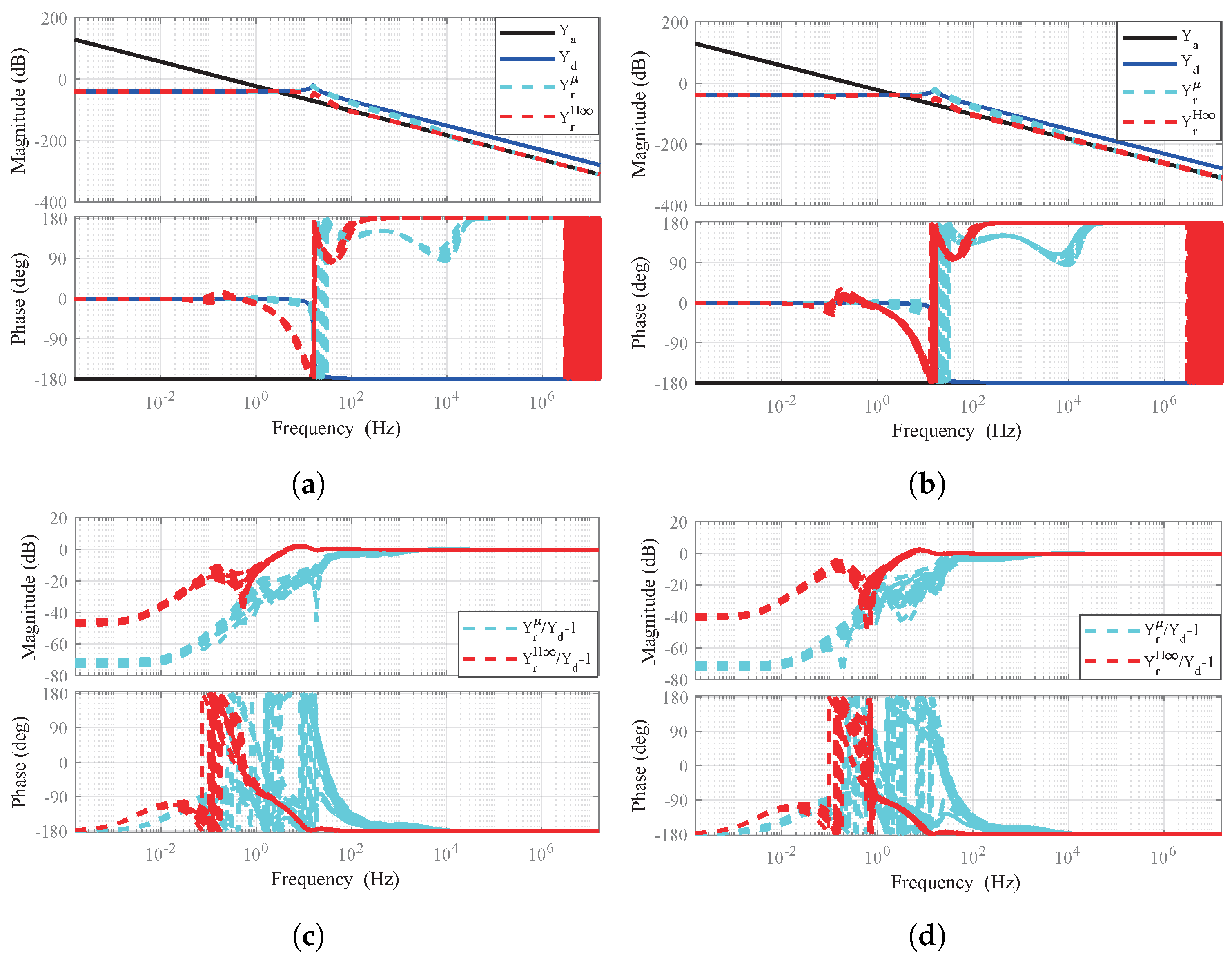
4.4. Comparative Analysis of Impedance Matching: $\mu$-Synthesis vs. ${\mathcal{H}}_{\infty }$ Control

To justify the selection of $\mathsf{\mu }$-synthesis over other robust control strategies, we provide a brief comparison with ${\mathcal{H}}_{\infty }$ control. Figure 7 presents a comprehensive frequency domain comparison of impedance rendering performance between $\mathsf{\mu }$-synthesis and ${\mathcal{H}}_{\infty }$ control strategies under structured parametric uncertainties in the joint inertia parameter J. Figure 7a,b shows the Bode plots of the rendered impedance values $Y_r^{\mu }$ and $Y_r^{\infty }$, implemented via $\mathsf{\mu }$-synthesis and ${\mathcal{H}}_{\infty }$ control, respectively, under 5% and 30% structured perturbations to the joint inertia. Both methods approximate the desired impedance profile, but $\mathsf{\mu }$-synthesis demonstrates superior fidelity, particularly in low−to−mid-frequency bands, where human–robot interaction performance is highly sensitive. Under increased uncertainty (30%), ${\mathcal{H}}_{\infty }$ control exhibits greater deviation of $Y_r^{\infty }$ from $Y_d$, with reduced phase stability and amplified gain variation, indicating a degradation in robustness.

Figure 7. Frequency – domain comparison of impedance matching performance between $\mathsf{\mu }$−synthesis and ${\mathcal{H}}_{\infty }$ control under structured joint inertia uncertainty. $Y_r^{\mu }$ and $Y_r^{\infty }$ represent the rendered impedance responses from the $\mathsf{\mu }$−synthesis and ${\mathcal{H}}_{\infty }$ controllers, respectively. (a,b) The Bode plots of rendered impedance $Y_r^{\mu }$ and $Y_r^{\infty }$ under 5% and 30% inertia perturbations, respectively. (c,d) The corresponding normalized impedance matching errors, defined as $Y_r^{\mu }/Y_d-1$ and $Y_r^{\infty }/Y_d-1$. The desired impedance $Y_d$ is specified by parameters $k_d=100\mathrm{Nm}/\mathrm{rad}$, $b_d=0.1\mathrm{Nm}/(\mathrm{rad}/\mathrm{s})$, and $m_d=0.01\mathrm{kg}·{\mathrm{m}}^2$. Results demonstrate that $\mathsf{\mu }$−synthesis achieves superior impedance matching fidelity and robustness under significant model uncertainty.

Figure 7c,d illustrates the normalized impedance matching errors, defined as $Y_r^{\mu }/Y_d-1$ and $Y_r^{\infty }/Y_d-1$, under $5\%$ and $30\%$ structured uncertainty, respectively. Compared to ${\mathcal{H}}_{\infty }$ control, the $\mathsf{\mu }$-synthesis approach reduces the impedance matching error magnitude by approximately $94.6\%$ and $97.5\%$ in the two cases, indicating a significant enhancement in both the precision and robustness of impedance rendering. Across the entire frequency range, the $\mathsf{\mu }$-synthesis controller consistently exhibits lower gain and phase errors, with particularly notable improvements under the $30\%$ perturbation condition, where it maintains phase coherence and bounded magnitude response. In contrast, the ${\mathcal{H}}_{\infty }$ controller shows substantial phase lag and gain peaking, especially in the high−frequency band. These results highlight the superior capability of $\mathsf{\mu }$-synthesis to maintain accurate and robust impedance shaping in the presence of structured dynamic uncertainties, thereby making it more suitable for safety−critical applications demanding high−fidelity physical interaction.

The $\mathsf{\mu }$-synthesis controller maintains smaller error magnitudes and more stable phase behavior under both 5% and 30% uncertainty conditions, demonstrating superior robustness and impedance rendering fidelity. These findings indicate that $\mathsf{\mu }$-synthesis is better suited for interaction−critical tasks requiring accurate and stable impedance shaping under model uncertainties.

4.5. Analysis of Critical Factors Influencing Impedance Matching Performance

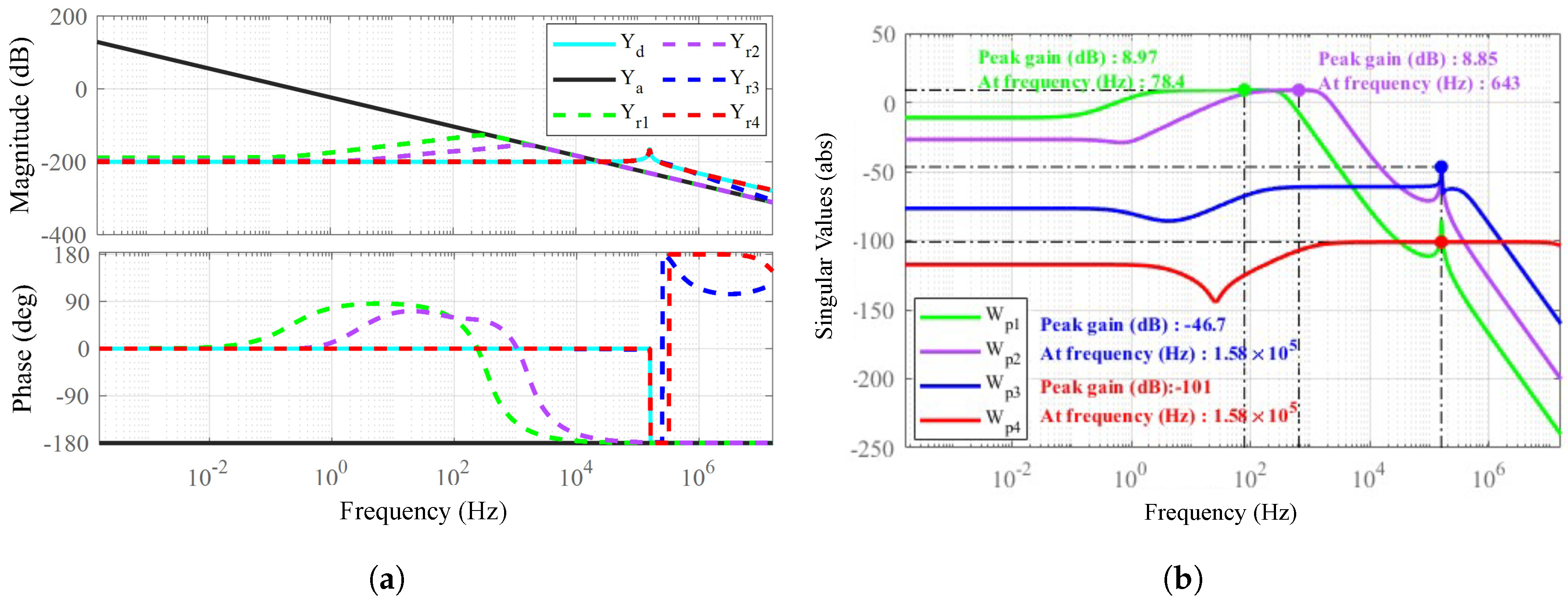
4.5.1. Effect of Performance Weighting Functions on Bandwidth

To systematically investigate the relationship between performance weighting functions and robustness characteristics in high−impedance regimes, this subsection analyzes frequency domain stability through the variation of singular values. Figure 8a demonstrates that the bandwidth of $W_{pi}$ fundamentally governs impedance matching capabilities, with broadband weightings enabling wider frequency coverage at the cost of high−frequency sensitivity. The constant weighting $W_{p4}$ achieves full−spectrum matching, while narrowband $W_{p1}$ prioritizes low−frequency precision but restricts impedance bandwidth.

Figure 8. Influence of different weighting functions $W_{pi}$, where the desired impedance parameters are $k_d={10}^{10}\mathrm{Nm}/\mathrm{rad}$, $b_d=0.1\mathrm{Nm}/(\mathrm{rad}/\mathrm{s})$, $m_d=0.01{\mathrm{kg}\text{·}\mathrm{m}}^2$; The performance weighting functions corresponding to $Y_{r1},Y_{r2},Y_{r3},$ and $Y_{r4}$ are $W_{p1}={10}^9/(0.1s+1)$, $W_{p2}={10}^9/(0.001s+1)$, $W_{p3}={10}^9/(0.00001s+1)$, and $W_{p4}={10}^9$, respectively. (a) Impedance matching. (b) Robust performance.

Figure 8b quantifies robust performance via structural singular value ($\mathsf{\mu }$) analysis. The peak gains of $W_{pi}$ explicitly reveal stability limitations: $W_{p1}$ and $W_{p2}$ exhibit critical violations at $8.97\mathrm{dB}$ and $8.85\mathrm{dB}$, respectively, failing the $\mu <1$ criterion across 78% of their spectra. In contrast, $W_{p3}$ and $W_{p4}$ demonstrate exceptional robustness with peak gains of $-46.7\mathrm{dB}$ and $-101\mathrm{dB}$, satisfying stability requirements with $34.7\mathrm{dB}$ and $58\mathrm{dB}$ margins. This stark contrast highlights the inherent trade−off between narrowband precision (high $\mathsf{\mu }$ peaks) and broadband stability. The results conclusively establish that weighting function design must prioritize singular value containment to ensure robust performance in high−impedance systems.

4.5.2. Impact of Joint Flexibility on Impedance Rendering Accuracy

This section discusses the impact of joint flexibility dynamics (3) on impedance rendering performance, as the inevitable flexible components in robotic joints influence system behavior. Figure 9 shows that the ideal rigid model achieves broader bandwidth matching under high−impedance conditions, while the flexible model is limited by factors such as sensor−actuator non−colocation. Increasing $k_d$ enhances system rigidity, thereby expanding the bandwidth. This effect is particularly pronounced in the rigid model, where higher values of $k_d$ substantially extend the impedance matching range. Despite the joint flexibility, the flexible model achieves high−accuracy impedance rendering within the frequency range of interest.

Figure 9. Effects of joint flexibility dynamics. $Y_{d1}$, $Y_{d2}$, and $Y_{d3}$, correspond to stiffness values of $k_d={10}^5$, ${10}^8$, and ${10}^9$ Nm/rad, respectively, with $b_d=0.1\mathrm{Nm}/(\mathrm{rad}/\mathrm{s})$ and $m_d=0.01\mathrm{kg}$. The weighting functions for the rigid and soft models are $W_p={10}^9$ and $W_p={\displaystyle \frac{{10}^4}{s^2+0.5s+1}}$, respectively.

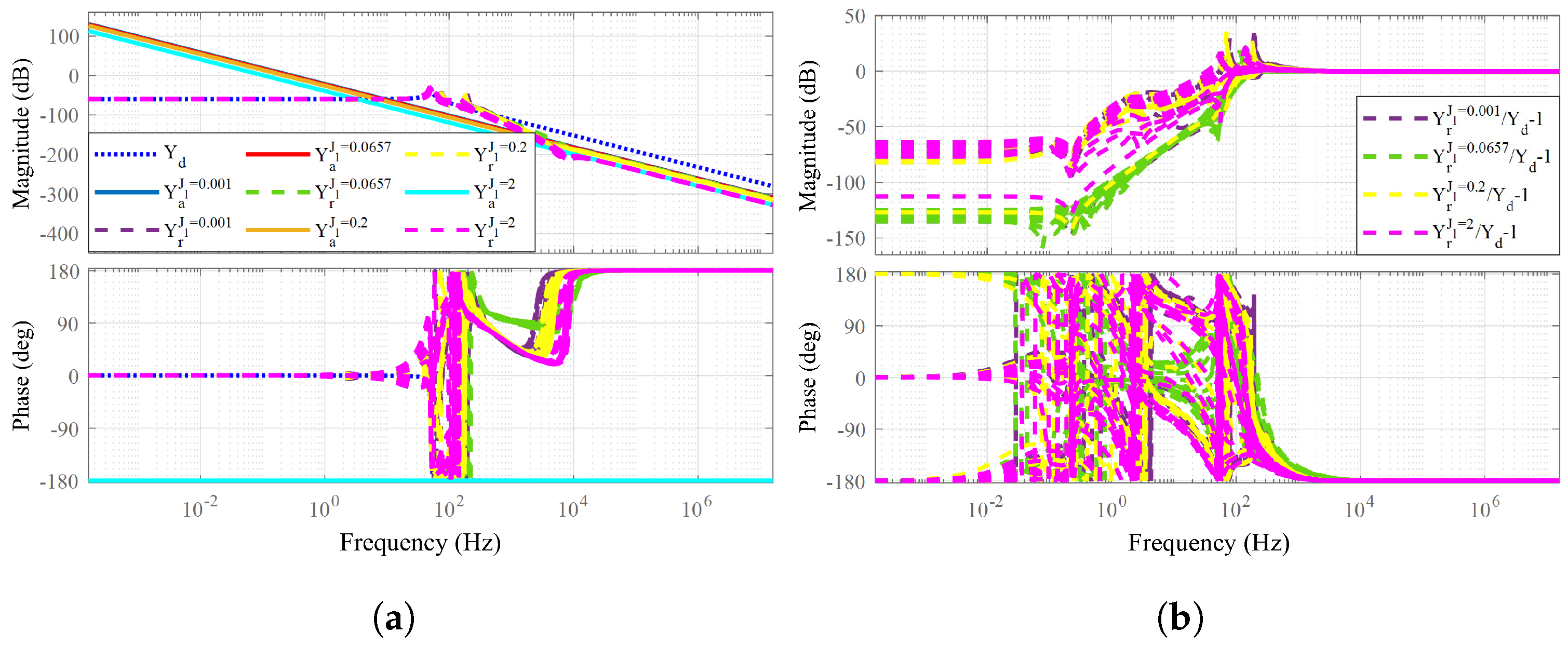
4.5.3. Influence of Load Inertia Variations on Impedance Matching Performance

To evaluate the influence of load inertia (structural uncertainty) variations on impedance matching fidelity, we conducted a series of simulations where the load−side link inertia $J_l$ was varied across a wide range, with 0.001, 0.0657, 0.2, and 2 kg$·$m² corresponding to different payloads and mechanical configurations. The goal was to assess how deviations from the nominal link inertia (0.0657 kg$·$m²) influence the impedance rendering accuracy.

Figure 10a presents the Bode plots of the impedance transfer function $Y_r$ rendered under different link inertias compared to the desired impedance $Y_d$, while Figure 10b quantifies the impedance matching error via normalized magnitude and phase deviations. Despite significant variations in $J_l$, the proposed $\mathsf{\mu }$-synthesis−based controller maintains high−fidelity impedance rendering across the entire frequency range. Particularly in low−frequency regions, which are critical for compliant interaction, the rendered impedance closely follows the desired profile, with only slight deviations as $J_l$ increases. Notably, even in extreme cases such as $J_l=2$ kg$·$m², the controller avoids significant peaking or phase lag that could compromise stability. This reflects the controller’s capacity to account for plant uncertainties and unmodeled dynamics through structured singular value ($\mathsf{\mu }$) optimization. Figure 10b further confirms that the normalized impedance error $Y_r^{I_l}/Y_d-1$ remains within acceptable bounds across all tested conditions, with minimal gain peaking. These results demonstrate that the proposed control architecture exhibits excellent robustness to inertia variations, ensuring consistent impedance matching performance under varying mechanical loads.

Figure 10. Comparison of impedance matching performance under different load inertia parameters with the desired impedance parameters $k_d=1000\mathrm{Nm}/\mathrm{rad}$, $b_d=0.1\mathrm{Nm}/(\mathrm{rad}/\mathrm{s})$, and $m_d=0.01{\mathrm{kg}\text{·}\mathrm{m}}^2$. (a) The impedance matching results. (b) The impedance matching error results.

4.5.4. Effect of Uncertainty Sources on Impedance Matching Performance

To validate the robustness of the proposed impedance control framework against various sources of uncertainties, multiple scenarios were simulated where the system was subjected to pure external disturbances, measurement noise, and actuator uncertainties. These conditions are representative of real−world interactions in uncertain environments, where noise and perturbations are inevitable.

Figure 11a compares the rendered impedance $Y_r$ under different uncertainty sources against the desired target impedance $Y_d$. The nominal rendered impedance $Y_{r,nom}$ (no uncertainty) case demonstrates excellent matching, while the introduction of disturbance ($Y_{r,dis}$), sensor noise ($Y_{r,n}$), and actuator uncertainty ($Y_{r,act}$) leads to slight deviations, particularly in mid− and high−frequency regions. However, the system preserves phase alignment and gain characteristics within practical tolerance levels, highlighting its robustness. Figure 11b presents the corresponding impedance matching errors, visualized through the normalized error transfer functions $Y_{r,i}/Y_d-1$. It is evident that among various sources of uncertainty, actuator uncertainties, measurement noise, and the combined effect of multiple uncertainties ($Y_{r,unc}$) have a more pronounced impact on the impedance mismatch. In contrast, the influence of external disturbances is relatively minor, especially at lower frequencies. This aligns with practical expectations, as actuator modeling errors often introduce multiplicative dynamics and delay, making them more challenging to suppress.

Figure 11. Comparison of impedance matching performance under the desired impedance parameters: $k_d=1000\mathrm{Nm}/\mathrm{rad}$, $b_d=0.1\mathrm{Nm}/(\mathrm{rad}/\mathrm{s})$, and $m_d=0.01{\mathrm{kg}\text{·}\mathrm{m}}^2$. (a) The rendered impedance matching to the desired impedance in scenarios with/without uncertainties, including pure disturbances, pure noise, and actuator uncertainties. (b) The corresponding impedance matching errors across different uncertainty sources.

Overall, the results confirm that the designed controller achieves reliable impedance rendering across a range of operational disturbances, maintaining system stability and interaction fidelity even in the presence of significant model and sensor uncertainties. This supports the applicability of the method to complex real−world robotic interaction scenarios.

4.6. Robots Interaction with the “Worst-Case” Environments

This section evaluates the influence of control parameters on interaction stability under the “worst-case” scenario, which represents the most unstable environmental conditions [36]. In this context, critical passive environments are modeled as a pure spring, characterized by driving point impedances of a/s, respectively. In the simulation, the environment (spring wall) stiffness is set to $k_e=1000\mathrm{Nm}/\mathrm{rad}$.

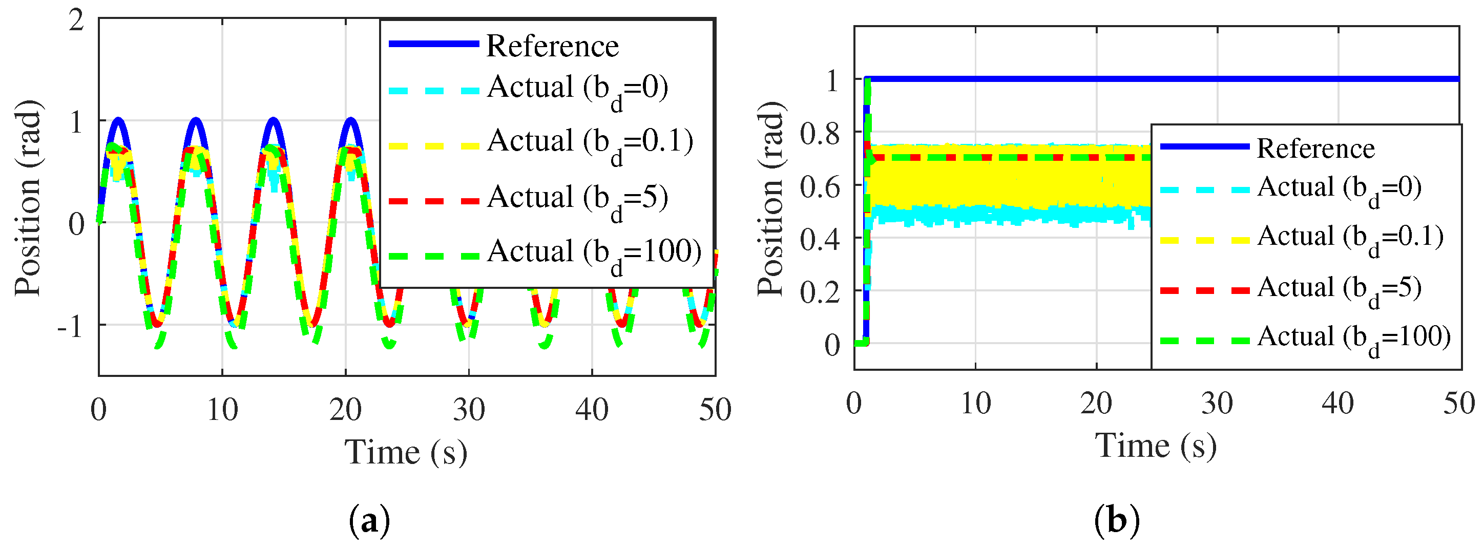
4.6.1. Impact of Virtual Damping on Control Performance

The introduction of $b_d$ is essential for mitigating oscillations and improving interaction stability. As shown in Figure 12a,b, the system’s response to sinusoidal and step reference signals demonstrates that, under conditions of $k_d=10\mathrm{Nm}/\mathrm{rad}$ and $b_d=0\mathrm{Nm}/(\mathrm{rad}/\mathrm{s})$, unstable interaction frequently occurs upon contact with the spring wall. When $b_d=0.1\mathrm{Nm}/(\mathrm{rad}/\mathrm{s})$, the oscillation amplitude decreases, indicating improved stability. Increasing $b_d=5\mathrm{Nm}/(\mathrm{rad}/\mathrm{s})$ effectively transitions the interaction from unstable to stable contact. However, an excessive damping value, such as $b_d=100\mathrm{Nm}/(\mathrm{rad}/\mathrm{s})$, results in degraded response performance.

Figure 12. Effect of $b_d$ on performance. The robot renders a lower desired stiffness of $k_d=10\mathrm{Nm}/\mathrm{rad}$, and $b_d$ is set to 0, 0.1, 5, and 100 Nm/(rad/s), respectively. (a) Tracking the sinusoidal signal $q_r=sin\left(t\right)$. (b) Tracking the step signal.

From the perspective of the desired impedance’s viscous component, selecting an appropriate level of $b_d$ is critical for balancing stability and response performance in interaction tasks.

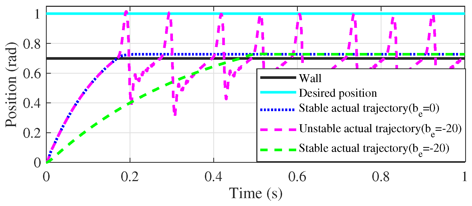
4.6.2. Contact with Viscoelastic Environments Featuring Negative Damping

To analyze the impact of negative damping in the environment on contact stability, we investigated the robot’s behavior during interaction with a viscoelastic wall. During contact, the robot exhibited oscillatory behavior characterized by alternating contact and separation, commonly referred to as contact instability [37]. Figure 13, shows when the environment damping ($b_e=-20\mathrm{Nm}/(\mathrm{rad}/\mathrm{s})$) exacerbates oscillatory behavior, significantly destabilizing the interaction. This instability arises from the amplification of energy dissipation inconsistencies caused by the negative damping, which prevents the system from achieving a stable equilibrium. To address this issue, the weighting function $W_p\left(s\right)={\displaystyle \frac{{10}^{-5}s+1000}{s+1.1\times {10}^{-5}}}$, stabilizing the interaction from unstable to stable contact.

Figure 13. Stable and unstable interactions with the wall. Where under the desired impedance $k_d=10\mathrm{Nm}/\mathrm{rad}$ and $b_d=20\mathrm{Nm}/(\mathrm{rad}/\mathrm{s})$, the robot’s response to a viscoelastic wall is analyzed to evaluate interaction stability.

The results underscore the importance of designing robust control strategies to counteract the adverse effects of negative damping, particularly in viscoelastic environments.

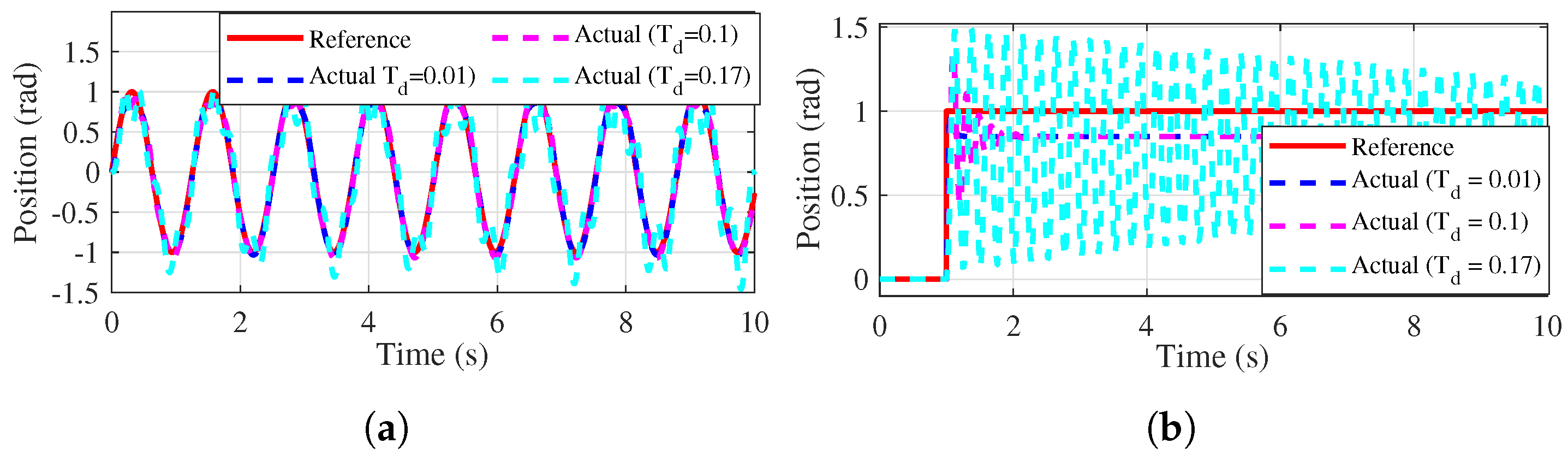
4.6.3. Effect of Actuator Phase Lag

To analyze the effects of actuator phase lag, the system’s responses to sinusoidal and step reference signals are shown in Figure 14a,b, respectively. The results reveal that excessive phase lag compromises both tracking accuracy and stability during physical interaction tasks. For impedance rendering, the control system remains stable under a phase lag associated with a time constant of $T_d=0.01\mathrm{s}$. Conversely, for trajectory tracking, the system demonstrates higher robustness, tolerating phase lag with a time constant up to $T_d=0.1\mathrm{s}$.

Figure 14. Effect of actuator phase lag. The robot’s desired impedance is designed as a pure virtual stiffness with $k_d=1000\mathrm{Nm}/\mathrm{rad}$. (a) Tracking the sinusoidal signal $q_r=sin\left(5t\right)$. (b) Tracking the step signal.

Actuator phase lag, characterized by a first-order time constant $T_d$, arises from intrinsic delays in actuator dynamics and critically impacts impedance control performance and stability.

4.7. Passivity Analysis

To analyze the passivity effect of the desired impedance on the robot’s rendered impedance, we evaluate the IFP index of the rendered impedance. Under passive conditions, the relative order of the analysis system is at most 1, and the robot’s desired, inherent, and rendered admittances are represented as $s{Y}_d$, $s{Y}_a$, and $s{Y}_r$, respectively. Figure 15 illustrates the frequency−dependent variation of the IFP index v under high− and low−stiffness impedance parameters. For high−stiffness impedance, $s{Y}_{d1}$ exhibits passivity excess, while $s{Y}_a$ shows a minor excess. In the controlled state, $s{Y}_{r1}$ maintains a robust passivity excess, particularly at low frequencies, ensuring stable interaction. Conversely, under low−stiffness impedance conditions, $s{Y}_{d2}$ demonstrates greater passivity excess, and $s{Y}_{r2}$ achieves excess primarily at higher frequencies.

Figure 15. Frequency–domain correlation of the input feedforward passivity index. The system transfer function is $W_p={\displaystyle \frac{9.9\times {10}^{4}s}{0.5s^2+100s+1}}$. For $Y_{d1}$, the parameters are $k_d={10}^9\mathrm{Nm}/\mathrm{rad}$, $b_d=0.1\mathrm{Nm}/(\mathrm{rad}/\mathrm{s})$, and $m_d=0.01\mathrm{kg}·{\mathrm{m}}^2$; for $Y_{d2}$, the parameters are $k_d=1\mathrm{Nm}/\mathrm{rad}$, $b_d={10}^4\mathrm{Nm}/(\mathrm{rad}/\mathrm{s})$, and $m_d=0.01\mathrm{kg}·{\mathrm{m}}^2$.

The analysis shows that, at the interaction port $(\dot{q},-{\tau }_e)$, the robot’s rendered impedance and the desired impedance can achieve passivity indices within the interested low−frequency range. The passivity index can be designed based on the desired impedance, ensuring that the rendered passivity index matches the desired passivity index.

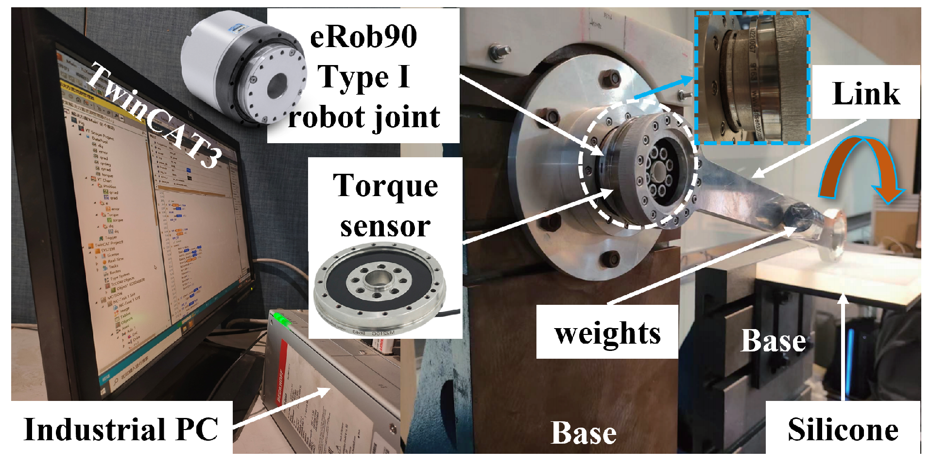
4.8. Experimental Setup

To evaluate the effectiveness of the proposed control methods, a series of experiments were conducted using a one−DoF modular robotic joint platform (see Figure 16). The experimental setup incorporates a ZeroErr eRob90N100I-BS-18ET actuator module (ZeroErr Technologies, Shenzhen, China), which features an integrated actuator with dimensions of $90\times 102\times 18$ mm and a mass of 2.1 kg. The actuator includes a precision harmonic drive with a 100:1 reduction ratio and a 20-bit multi-turn encoder, offering a repeatability of $\pm 7$ arcsec and an absolute accuracy of $\pm 15$ arcsec. The control system consists of a Beckhoff C6930-0060 industrial PC (Intel Core i5-4400E @ 2.7 GHz, Beckhoff Automation, Verl, Germany), a C9900-L100 license key USB stick for TwinCAT 3.1 (Beckhoff Automation, Verl, Germany), and EtherCAT-based I/O peripherals including an EK1100 coupler, EL3102 analog input terminal, and EL9011 end terminal. Real-time control was implemented using MATLAB 2018b and Simulink xPC Target at a sampling frequency of 1 kHz. Torque measurement employs a SUNRISE M2210G7 sensor (Sunrise Instruments, Nanning, China), which features a measurement range of 0–100 Nm, a torsional stiffness of $1.7\times {10}^6$ Nm/rad, and a sensitivity of $1.1588\times {10}^{-2}$ V/EU. The sensor exhibits nonlinearity of $\pm 0.08\%$ FS and hysteresis of $\pm 0.06\%$ FS. In the experiments, silica gel with Shore A hardness of ${10}^{\circ }$ served as the interaction object, simulating soft material contact.

Figure 16. 1-DoF modular robotic joint experimental setup.

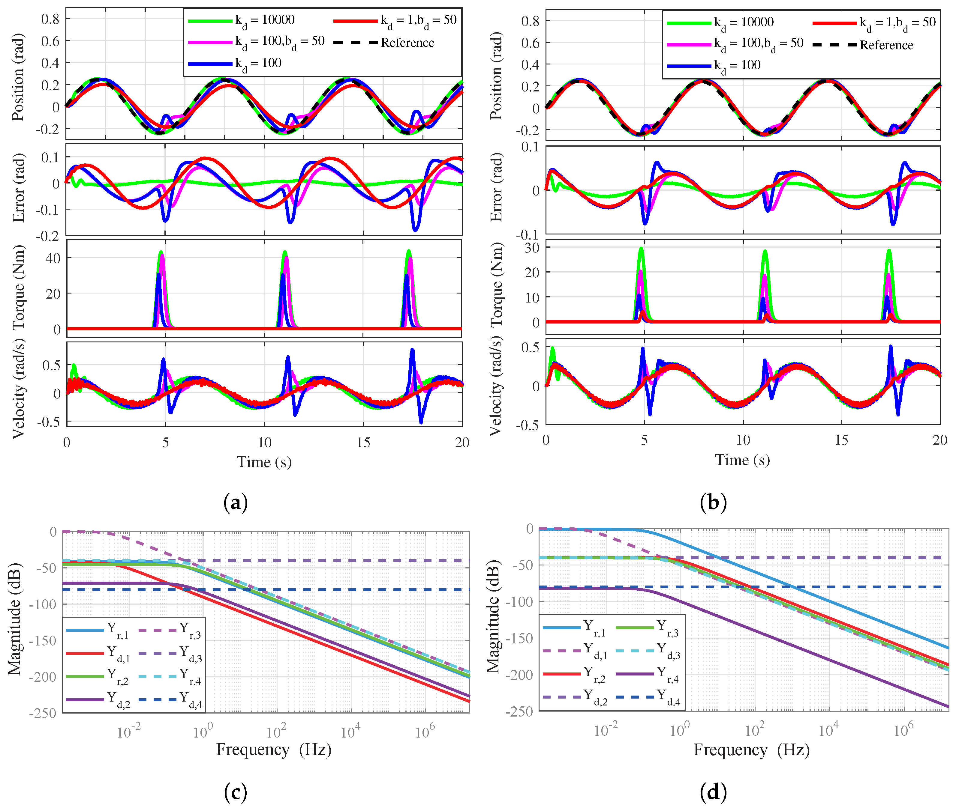
4.9. Experiments: Comparison of Contact Performance

This section evaluates the effectiveness of the proposed robust impedance control (RIC) in comparison to classical impedance control (CIC), with a focus on impedance rendering performance and interaction stability.

Figure 17a illustrates the control performance of CIC, revealing poor position tracking accuracy during free−space motion and pronounced instability in constrained motion, particularly under low−stiffness and zero−damping conditions. Although CIC theoretically satisfies passivity conditions under ideal circumstances or with appropriately tuned impedance parameters, but practical issues such as parameter perturbations, disturbances, and sensor noise can cause stored energy to exceed dissipated energy, violating passivity. In contrast, Figure 17b shows that the proposed RIC achieves improved tracking in free−space motion, reduced contact forces, and stable interactions by maintaining passivity, particularly in low impedance scenarios. At low frequencies, stiffness−dominated impedance behavior is observed, while contact rebound under low stiffness highlights the necessity for additional damping to maintain contact stability.

Figure 17. Experimental comparison of classical and robust impedance control. (a) Time domain contact performance of classical impedance control (CIC). (b) Time domain contact performance of robust impedance control (RIC). (c) Frequency domain impedance matching results of CIC. (d) Frequency domain impedance matching results of RIC. The results demonstrate the performance difference between the two control methods in both time and frequency domains.

The System Identification Toolbox in MATLAB 2018b is employed to analyze the time domain impedance rendering results, yielding the corresponding frequency domain impedance characteristics. The impedance rendering accuracy in the frequency domain is illustrated in Figure 17c,d show the frequency domain results for the desired impedance rendered by CIC and RIC, respectively. For CIC, the IMA reaches 0.9914 under low stiffness ($k_d=1\mathrm{Nm}/\mathrm{rad},b_d=50\mathrm{Nm}/(\mathrm{rad}/\mathrm{s})$) but deteriorates significantly under higher stiffness or zero damping (IMA = 0.4380 at $k_d=100\mathrm{Nm}/\mathrm{rad}$ without damping). At extreme stiffness ($k_d=10,000\mathrm{Nm}/\mathrm{rad}$), IMA becomes 1.7966 due to the difficulty in matching high-stiffness impedance. In contrast, RIC presents more conservative behavior: IMA remains low (0.4425, 0.0023, and 0.1994 for increasing stiffness levels) but exhibits more consistent impedance rendering across medium−stiffness configurations.

To quantify this improvement, Table 4 reports the impedance matching accuracy (IMA) values under both control schemes and the corresponding error reduction (%). Comparatively, RIC reduces the impedance rendering error by an average of 85.71% across all tested configurations relative to CIC while maintaining superior passivity and robustness. This highlights the controller’s trade−off strategy: rather than aggressively matching the desired impedance at all costs, RIC prioritizes safe and stable interaction by attenuating non−minimum phase effects and accommodating system limitations. From a physical viewpoint, this ensures more predictable energy behavior during contact transitions, especially under uncertainty or parameter perturbations.

Table 4. Impedance Matching Accuracy (IMA) and Error Reduction Comparison.

${\mathit{k}}_{\mathit{d}}$ (Nm/rad)	${\mathit{b}}_{\mathit{d}}$ (Nm/(rad/s))	IMA (CIC)	IMA (RIC)	Error Reduction (%)
1	50	0.9914	0.4425	55.36
100	0	0.4380	0.0023	99.47
100	50	0.4630	0.0042	99.09
10,000	0	1.7966	0.1994	88.90

In summary, CIC achieves high impedance fidelity only under idealized conditions but suffers from degraded stability in practical environments. The proposed RIC approach, although sacrificing some fidelity, provides enhanced robustness, reliable tracking, and stable contact interactions, making it well suited for applications requiring compliant behavior and safe physical human–robot interactions.

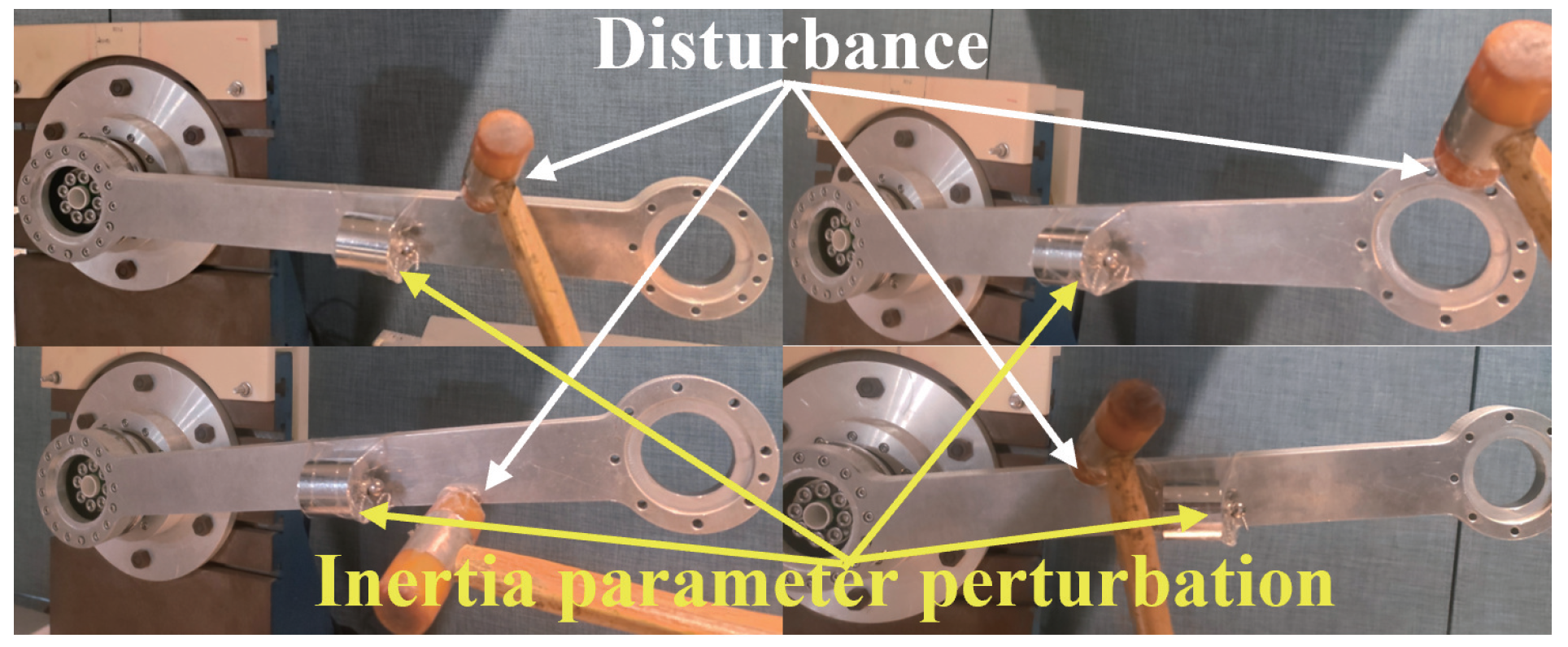
4.10. Experiments: Robustness Verification

To assess the robustness of the proposed controller under varying interaction environments, a series of disturbance rejection tests were performed on the one−DoF robotic joint with a fixed rigid link, where different desired impedance levels were rendered to emulate diverse environmental stiffness conditions. Although the physical load remained rigid, the controller modulated the apparent joint impedance from compliant to stiff, effectively simulating a range of interaction scenarios without altering the hardware configuration.

Random impulsive disturbances were introduced by striking the joint link with a rubber hammer (see Figure 18), mimicking unexpected contact events or environmental perturbations. During the test, the system operated under the robust impedance control mode, and sensor data were recorded to monitor deviations in joint position and interaction force. The results show that the proposed controller effectively suppressed transient deviations, with rapid return to the desired trajectory and force equilibrium. No oscillations or instability were observed, demonstrating strong robustness against abrupt external disturbances. These findings reinforce the practical applicability of the control strategy in dynamic and uncertain environments.

Figure 18. Random disturbance application using a rubber hammer on the robotic joint.

Additionally, parametric uncertainty was considered by attaching weights at the link end to vary the effective inertia. Figure 19 illustrates the effect of different desired stiffness values ($k_d=1$, 10, 100, 1000, and 10,000 Nm/rad) with a fixed damping coefficient ($b_d=50$ Nm/(rad/s)). The position is a continuous function of time, and in trajectory tracking, the goal is to closely follow the reference trajectory $q_r\left(t\right)$. To evaluate performance, we used the mean absolute position error

$$e:={\displaystyle \frac{1}{T}}{\int }_0^T|q\left(t\right)-q_r\left(t\right)|dt,$$

(29)

where T is the measurement duration and the $L_1$-norm is used for e instead of the $L_2$-norm to equally weight low and high errors in the performance index.

Figure 19. Robust performance under disturbances. With $b_d=50$ Nm/(rad/s) and $k_d$ values of 1, 10, 100, 1000 and 10,000 Nm/rad, $e\left({10}^{-3}\right)$ are 4.539, 3.428, 2.220, 0.7998 and 0.4062 rad, respectively.

The results confirm that higher stiffness rendering significantly improves disturbance rejection and tracking accuracy, reducing e from 4.539 to 0.4062 rad as $k_d$ increases; higher stiffness values yield minimal errors, showcasing improved robustness, while intermediate stiffness reveals a trade−off between compliance and a rejection of disturbances. This demonstrates that the controller maintains robustness across a wide range of emulated environment dynamics, from soft to stiff impedance settings, despite physical interaction remaining with a rigid load. Furthermore, no instability or oscillation was observed throughout the tests, highlighting the proposed method’s effectiveness under both compliant−like and stiff−like virtual interaction conditions.

4.11. Discussion

The experimental and simulation results demonstrate that the proposed $\mathsf{\mu }$-synthesis framework significantly advances impedance control performance in three critical dimensions, namely accuracy, bandwidth, and robustness. By explicitly modeling structured uncertainties, including $\pm 30\%$ inertia variations, $\pm 5\%$ stiffness perturbations, and high−frequency sensor noise, the controller significantly improves impedance matching accuracy while maintaining closed−loop stability. This improvement is attributed to the systematic optimization of the structured singular value ($\mathsf{\mu }$) in the frequency domain, which minimizes worst−case rendering errors through robust ${\mathcal{H}}_{\infty }$ norm constraints. The framework demonstrates particular effectiveness in high−stiffness rendering scenarios, where it suppresses instability modes caused by unmodeled dynamics and sensor noise, outperforming conventional approaches in both transient and steady−state responses.

Target impedance selection critically shapes closed−loop behavior through frequency domain characteristics and time domain constraints. The low−pass profile ensures compliant interaction via low−frequency stiffness/damping while attenuating high−frequency disturbances. From the time domain perspective, the target stiffness $k_d$ influences the position deviation under sustained forces, while the damping coefficient $b_d$ regulates velocity overshoot and energy absorption during transient contact. Selecting overly stiff impedance may improve tracking accuracy but could risk unsafe high−contact forces during human–robot interactions. Conversely, underdamped impedance may cause oscillatory responses.

Implementation considerations reveal critical tradeoffs. A critical advantage of joint−space impedance control implementation lies in its reduced sensitivity to kinematic model errors compared to cartesian−space approaches. While end−effector impedance control enables direct task space specification, its dependence on accurate Jacobian matrices introduces configuration-dependent uncertainties, particularly problematic in modular joints with variable payloads. Our joint-level formulation avoids these complications through decentralized dynamics modeling, though at the cost of requiring higher actuator bandwidth to compensate for inertial coupling effects. The simulation validation with $\pm 30\%$ payload variations demonstrates the framework’s capability to maintain stability without reconfiguration. Additionally, actuator saturation is a critical constraint in high−performance impedance control. Excessive commanded torques, particularly during sudden contact or large perturbations, may exceed motor limits, leading to performance degradation or instability. In our implementation, saturation bounds are explicitly considered in the synthesis process to ensure bounded control outputs under worst−case uncertainties.

The proposed controller addresses model uncertainties and prevents overfitting through a dual strategy combining frequency domain regularization and structured robustness validation. To avoid overfitting to specific uncertainty scenarios, frequency−dependent weighting functions are employed as regularization mechanisms: a low−pass performance weight prioritizes low−frequency tracking accuracy while naturally attenuating unmodeled high−frequency dynamics, and a high−pass control effort weight limits actuator signal amplification at frequencies beyond the system’s bandwidth. The controller’s anti−overfitting strategy combines frequency domain regularization with structured robustness validation. Low−pass performance weights prioritize tracking accuracy below 50 rad/s, naturally attenuating unmodeled high−frequency dynamics, while high−pass effort weights limit actuator amplification beyond system bandwidth. This regularization enables consistent performance across uncertainty scenarios without parameter retuning.

The generalization capability of the proposed robust impedance control framework to different robotic platforms and configurations is a crucial consideration for its practical deployment. The controller formulation is model−based, and its design is parameterized based on the system dynamics and interaction characteristics, which ensure its scalability and adaptability to various robot morphologies. While the experiments in this study were conducted on a one−DoF modular joint platform, the underlying principles of structured uncertainty modeling and $\mathsf{\mu }$-synthesis are not limited to this configuration. The $\mathsf{\mu }$-synthesis−based approach, with its frequency domain design process and structured uncertainty handling, is inherently suited for extension to multi−DoF systems. The key requirement for successful generalization is an accurate system model, which includes the characterization of both the robot’s dynamics and the expected interaction conditions. For example, the uncertainty bounds in the joint dynamics must be well defined for higher−DoF systems, and the control framework can then be adjusted to account for more complex kinematics and dynamics associated with the multi−DoF configuration. One practical concern of applying $\mathsf{\mu }$-synthesis in high−DoF robotic systems is the increased computational burden arising from the D−K iteration loop and the size of the structured uncertainty matrices. The complexity of solving the $\mathsf{\mu }$ upper bound optimization problem grows with system dimensionality, which can pose challenges for real−time applications. Additionally, controller order reduction techniques, such as balanced truncation or Hankel norm approximation, can be applied after D−K iteration to obtain a reduced−order controller that retains essential robustness characteristics. These strategies enable the deployment of $\mathsf{\mu }$-synthesis−based impedance control in higher-DoF systems while maintaining real−time performance.

In the context of human–robot interactions (HRIs), the proposed robust impedance controller offers a promising foundation. Its inherent passivity and disturbance rejection capabilities make it suitable for safe physical collaboration tasks, such as assistive manipulation, rehabilitation, or shared control scenarios. However, real−time adaptation to user intent, motion variability, and safety constraints remains an open challenge. Integration with intent estimation modules or biomechanical feedback loops may further improve responsiveness and personalization in HRI contexts.

5. Conclusions

In this work, we reformulate the impedance control of robots under structural uncertainty within a general impedance matching framework, where the system’s impedance dynamics are shaped to align with a predefined impedance model. The proposed approach effectively shapes the robot’s closed−loop impedance to match a desired model while accounting for dynamic parameter variations, sensor noise, and actuator dynamics. By minimizing the structured singular value in the frequency domain, the controller achieves accurate and stable impedance rendering across a wide frequency range. The analysis of the frequency dependence of rendering the desired impedance reveals that the impedance matching bandwidth is fundamentally constrained by the robot’s inherent dynamics. In essence, impedance rendering is bandwidth−limited, meaning that the actual impedance produced by the robot can be approximated as a combination of desired impedance in the low−frequency range and inherent impedance in the high−frequency range. By fine−tuning of the performance weighting functions and selection of appropriate impedance parameters, the proposed approach effectively achieved frequency domain impedance control. This is realized by minimizing the maximum structural singular value within a robust control framework, which quantifies the frequency domain error between the rendered and desired impedance.

However, challenges remain in extending the approach to multi−DoF robotic systems due to the coupled dynamics and the computational burden of D−K iteration. Real-time implementation on embedded platforms also requires efficient numerical methods or hardware acceleration. Future work will address these issues by exploring scalable synthesis techniques, decentralized or hierarchical control architectures, and deployment strategies for embedded systems. The method’s passivity−aware and frequency−weighted robustness design makes it well−suited for physical human−robot interactions (pHRIs), rehabilitation robotics, haptic rendering, and variable impedance tasks, offering stable, energy−efficient interaction in compliant and uncertain environments.

References

- Billard, A.; Kragic, D. Trends and challenges in robot manipulation. Science 2019, 364, eaat8414. [Google Scholar] [CrossRef] [PubMed]
- Hogan, N.; Buerger, S.P. Impedance and interaction control. In Robotics and Automation Handbook; CRC Press: Boca Raton, FL, USA, 2018; pp. 375–398. [Google Scholar]
- Hogan, N. Impedance control—An approach to manipulation. I—Theory. II—Implementation. III—Applications. J. Dyn. Syst. Meas. Control 1985, 107, 1–24. [Google Scholar] [CrossRef]
- Albu-Schäffer, A.; Ott, C.; Hirzinger, G. A unified passivity-based control framework for position, torque and impedance control of flexible joint robots. Int. J. Robot. Res. 2007, 26, 23–39. [Google Scholar] [CrossRef]
- Valency, T.; Zacksenhouse, M. Accuracy/Robustness Dilemma in Impedance Control. J. Dyn. Syst. Meas. Control 2003, 125, 310–319. [Google Scholar] [CrossRef]
- Siciliano, B.; Villani, L. Robot Force Control; Springer: New York, NY, USA, 1999. [Google Scholar]
- Lawrence, D. Impedance Control Stability Properties in Common Implementations. In Proceedings of the 1988 IEEE International Conference on Robotics and Automation, Philadelphia, PA, USA, 24–29 April 1988; Volume 2, pp. 1185–1190. [Google Scholar] [CrossRef]
- Hogan, N. Contact and physical interaction. Annu. Rev. Control Robot. Auton. Syst. 2022, 5, 179–203. [Google Scholar] [CrossRef]
- Tosun, F.E.; Patoglu, V. Necessary and sufficient conditions for the passivity of impedance rendering with velocity-sourced series elastic actuation. IEEE Trans. Robot. 2020, 36, 757–772. [Google Scholar] [CrossRef]
- Hace, A.; Uran, S.; Jezernik, K.; Curk, B. Robust Sliding Mode Based Impedance Control. In Proceedings of the IEEE International Conference on Intelligent Engineering Systems, Budapest, Hungary, 15–17 September 1997; pp. 77–82. [Google Scholar] [CrossRef]
- Lu, Z.; Goldenberg, A.A. Robust impedance control and force regulation: Theory and experiments. Int. J. Robot. Res. 1995, 14, 225–254. [Google Scholar]
- Kelly, R.; Carelli, R.; Amestegui, M.; Ortega, R. On Adaptive Impedance Control of Robot Manipulators. In Proceedings of the 1989 International Conference on Robotics and Automation, Scottsdale, AZ, USA, 14–19 May 1989; Volume 1, pp. 572–577. [Google Scholar] [CrossRef]
- Izadbakhsh, A.; Khorashadizadeh, S. Robust impedance control of robot manipulators using differential equations as universal approximator. Int. J. Control 2018, 91, 2170–2186. [Google Scholar] [CrossRef]
- Zhou, K.; Doyle, J.C. Essentials of Robust Control; Prentice Hall Upper: Saddle River, NJ, USA, 1998; Volume 104. [Google Scholar]
- Packard, A.K. What’s New With Mu: Structured Uncertainty in Multivariable Control; University of California: Berkeley, CA, USA, 1988. [Google Scholar]
- Zhang, S.Y.; Hui, Z.; Huang, Q.T. Application of μ theory in compliant force control. Chin. J. Aeronaut. 2006, 19, 89–96. [Google Scholar] [CrossRef]
- Uchimura, Y.; Kazerooni, H. A μ-Synthesis Based Control for Compliant Maneuvers. J. Dyn. Syst. Meas. Control 2006, 128, 914–921. [Google Scholar] [CrossRef]
- Aghili, F. Robust Impedance-Matching of Manipulators Interacting With Uncertain Environments: Application to Task Verification of the Space Station’s Dexterous Manipulator. IEEE/ASME Trans. Mechatronics 2019, 24, 1565–1576. [Google Scholar] [CrossRef]
- Fotuhi, M.J.; Ben Hazem, Z.; Bingül, Z. Modelling and Torque Control of an Non-Linear Friction Inverted Pendulum Driven with a Rotary Series Elastic Actuator. In Proceedings of the 2019 3rd International Symposium on Multidisciplinary Studies and Innovative Technologies (ISMSIT), Ankara, Turkey, 11–13 October 2019; pp. 1–6. [Google Scholar] [CrossRef]
- Guo, X.; Volery, M.; Lissek, H. PID-like active impedance control for electroacoustic resonators to design tunable single-degree-of-freedom sound absorbers. J. Sound Vib. 2022, 525, 116784. [Google Scholar] [CrossRef]
- Kim, W.; Lee, D.; Yun, D.; Ji, Y.; Kang, M.; Han, J.; Han, C. Neurorehabilitation Robot System for Neurological Patients Using H-Infinity Impedance Controller. In Proceedings of the 2015 IEEE International Conference on Rehabilitation Robotics (ICORR), Singapore, 11–14 August 2015; pp. 876–881. [Google Scholar] [CrossRef]
- Ott, C.; Albu-Schaffer, A.; Kugi, A.; Hirzinger, G. On the Passivity-Based Impedance Control of Flexible Joint Robots. IEEE Trans. Robot. 2008, 24, 416–429. [Google Scholar] [CrossRef]
- Losey, D.P.; Erwin, A.; McDonald, C.G.; Sergi, F.; O’Malley, M.K. A Time-Domain Approach to Control of Series Elastic Actuators: Adaptive Torque and Passivity-Based Impedance Control. IEEE/ASME Trans. Mechatronics 2016, 21, 2085–2096. [Google Scholar] [CrossRef]
- Lee, H.; Lee, J.; Keppler, M.; Oh, S. Robust Elastic Structure Preserving Control for High Impedance Rendering of Series Elastic Actuator. IEEE Robot. Autom. Lett. 2024, 9, 3601–3608. [Google Scholar] [CrossRef]
- Yu, N.; Zou, W.; Tan, W.; Yang, Z. Augmented virtual stiffness rendering of a cable-driven SEA for human-robot interaction. IEEE/CAA J. Autom. Sin. 2017, 4, 714–723. [Google Scholar] [CrossRef]
- Haddadin, S.; De Luca, A.; Albu-Schäffer, A. Robot collisions: A survey on detection, isolation, and identification. IEEE Trans. Robot. 2017, 33, 1292–1312. [Google Scholar] [CrossRef]
- Griggs, W.M.; Anderson, B.D.; Shorten, R.N. A test for determining systems with “mixed” small gain and passivity properties. Syst. Control Lett. 2011, 60, 479–485. [Google Scholar] [CrossRef]
- Xia, M.; Antsaklis, P.J.; Gupta, V.; Zhu, F. Passivity and dissipativity analysis of a system and its approximation. IEEE Trans. Autom. Control 2016, 62, 620–635. [Google Scholar] [CrossRef]
- Huang, Y.; Huang, Q. Interaction Stability Analysis from the Input-Output Viewpoints. In Proceedings of the 2020 IEEE International Conference on Robotics and Automation (ICRA), Paris, France, 31 May–31 August 2020; pp. 7878–7884. [Google Scholar]
- Huang, Y.; Li, S.; Huang, Q. Robust impedance control for SEAs. J. Frankl. Inst. 2020, 357, 7921–7943. [Google Scholar] [CrossRef]
- Huang, Y.C.; Shao, N.F. LMI-based impedance control synthesis: A case study on fixed-stiffness actuators (FSAs). Int. J. Control 2023, 96, 2945–2957. [Google Scholar] [CrossRef]
- Huo, L.; Qu, C.; Li, H. Robust control of civil structures with parametric uncertainties through D-K iteration. Struct. Des. Tall Spec. Build. 2016, 25, 158–176. [Google Scholar] [CrossRef]
- Keemink, A.Q.; Van der Kooij, H.; Stienen, A.H. Admittance control for physical human–robot interaction. Int. J. Robot. Res. 2018, 37, 1421–1444. [Google Scholar] [CrossRef]
- Packard, A.; Doyle, J. The complex structured singular value. Automatica 1993, 29, 71–109. [Google Scholar] [CrossRef]
- Skogestad, S.; Postlethwaite, I. Multivariable Feedback Control: Analysis and Design; John Wiley & Sons: Hoboken, NJ, USA, 2005. [Google Scholar]
- Colgate, J.E.; Hogan, N. Robust control of dynamically interacting systems. Int. J. Control 1988, 48, 65–88. [Google Scholar] [CrossRef]
- Colgate, E.; Hogan, N. An Analysis of Contact Instability in Terms of Passive Physical Equivalents. In Proceedings of the 1989 International Conference on Robotics and Automation, Scottsdale, AZ, USA, 14–19 May 1989; pp. 404–409. [Google Scholar]
Disclaimer/Publisher’s Note: The statements, opinions and data contained in all publications are solely those of the individual author(s) and contributor(s) and not of MDPI and/or the editor(s). MDPI and/or the editor(s) disclaim responsibility for any injury to people or property resulting from any ideas, methods, instructions or products referred to in the content. |
© 2025 by the authors. Licensee MDPI, Basel, Switzerland. This article is an open access article distributed under the terms and conditions of the Creative Commons Attribution (CC BY) license (https://creativecommons.org/licenses/by/4.0/).