Comparative Study of Analytical Model Predictive Control and State Feedback Control for Active Vibration Suppression of Two-Mass Drive

Abstract

This article discusses speed control methods for electric motor drives with elastic mechanical coupling causing torsional vibrations, which negatively affect the operation of the system. Model Predictive Control (MPC) is often presented as an effective solution; however, it is notoriously difficult to implement in real-time due to the high computational complexity of the controller. In this paper, a simplified predictive control approach in the form of Analytical MPC (aMPC) is proposed for the speed control of a two-mass motor drive. In contrast to conventional MPC, which requires complex online optimisation, aMPC derives an explicit control law analytically under simplifying assumptions, greatly reducing the computational load. The effect of the controller parameters on the drive performance is investigated and a multi-objective performance function for automatic tuning is proposed. The aMPC structure is compared with conventional State Feedback Control (SFC), including a system robustness test of both approaches. Based on simulation studies and experimental verification, the proposed structure is shown to ensure high dynamics in drive control, with smoother torque control and superior robustness for higher-load inertia ratios than SFC.

1. Introduction

In contemporary industrial systems, electrical drives are required to operate with high dynamics and precision. These systems are typically modelled under the assumption of a perfectly rigid connection between the motor drive and the load. This assumption is convenient and effective in cases where the system dynamics are relatively straightforward and do not involve significant resonant behaviours. The utilisation of a one-mass motor drive model is common practice, particularly in conjunction with Proportional-Integral (PI) or Proportional-Integral-Derivative (PID) controllers, which have garnered widespread acceptance due to their inherent simplicity and ease of implementation [1].

However, in certain industrial applications, the consequences of neglecting the finite stiffness of the shaft can be significant. In systems demanding high precision—e.g., robot manipulators or rolling mill drives—the elasticity of coupling can result in resonance, manifesting as torsional vibrations [2]. Such vibrations can also be generated as a consequence of external disturbances on the load, for example in the case of wind turbines or electric vehicle drives [3]. This can lead to inaccuracies in position or speed control, and even mechanical damage to the drive system. In such cases, a two-mass system is a more appropriate model, in which the motor and the load are regarded as separate inertial masses connected by an elastic coupling.

Despite their effectiveness in a broad range of applications, PI/PID controllers struggle to manage the complexities associated with resonant systems. This is because the closed-loop system is fourth order, which exceeds the number of available controller parameters [4,5]. Consequently, it is not possible to independently locate all four poles of the system, and traditional PI-based cascade structures, utilising classical tuning criteria, are incapable of effectively suppressing torsional oscillations [6].

The most prominent alternative tuning methods involve pole configurations with an identical real part, resonant frequency, or damping factor. However, as concluded by the authors of [7,8], different methods for pole assignment must be used depending on the inertia ratio of the system. A more suitable approach involves the incorporation of additional feedback loops into the control structure, which allows for an increased number of control parameters. However, this solution relies heavily on the accurate estimation of drive parameters and additional drive state variables [9].

Another prevalent method of achieving the desired drive speed control performance is the application of State Feedback Control (SFC). It has been demonstrated that SFC can provide the satisfactory suppression of torsional vibrations [10]. A primary disadvantage is that all the parameters of the controller must be tuned simultaneously, which results in a complex and time-consuming tuning process. However, in recent years, methods for an automatic tuning process have been proposed [11,12]. Other methodologies involving independent pole location include Forced Dynamic Control (FDC), where the closed-loop system is designed to follow specific linear or non-linear dynamic behaviours [13].

In two-mass systems, the load moment of inertia may vary over time due to the nature of the load machine. To ensure the proper system response, adaptive and robust control methods are often recommended in the literature. An example of this trend is shown in [14], where the authors modified a PI controller with additional feedback by introducing pattern-search optimisation tuning. A control strategy known to be robust is Sliding-Mode Control (SMC), which yields satisfactory vibration suppression, but comes with a drawback in the form of chattering [15,16].

Contemporary approaches in recent years often incorporate elements of fuzzy logic or neural networks and frequently combine the advantages of both, as demonstrated in SMC-based neuro-fuzzy control [17]. The method proposed in [18] integrates fuzzy logic with an adaptive controller to improve the suppression of mechanical vibrations. The application of deep learning approaches in two-mass drives is explored in [19], with four structures used for state variable estimation.

The primary disadvantage of the aforementioned control methods is their inability to predict and compensate for future system behaviour. This can lead to the poor handling of resonance suppression and may result in increased overshooting, oscillations, and an overall decrease in the dynamic performance of the control system [20].

In addressing the challenges posed by two-mass dynamics, Model Predictive Control (MPC) has emerged as an advanced and effective solution. This control strategy relies on the model of the system to predict its future behaviour and optimise control signals in real-time [21]. In this way, it can anticipate the effect of future disturbances and its own control signal to reduce errors in speed or position [22], while also mitigating undesirable behaviours, such as torsional oscillations [23].

Additionally, MPC facilitates the incorporation of constraints on the internal state variables, such as torque or velocity limits, and safety margins, which are critical in industrial systems to avert damage or failure [24]. Particularly beneficial in the case of two-mass drives, MPC allows for constraining torsional torque during the design phase of the controller.

However, the implementation of a predictive algorithm requires substantial computational effort, as it relies on solving complex optimisation problems in real-time. The practical implementation of MPC in this form for systems with small time constants is usually impractical due to the comparatively long time of the calculations performed. This limits the scope of the application of the online MPC control to objects with relatively large time constants [25].

Predictive control for dynamic real-world applications can be successfully implemented with the use of Explicit Model Predictive Control (eMPC), in which, for a given objective function, the entire calculation process is carried out offline for all combinations of an adopted state vector. Therefore, the control is reduced to a simple look-up table. This allows for the practical implementation of complex constraint-sensitive predictive control, even in demanding systems with small sampling steps [26]. However, since the optimal control signals are only calculated for predetermined conditions, eMPC might not provide robustness or even stability in unforeseen circumstances, e.g., dynamic parameter changes of the plant parameters.

In recent years, Deep Neural Networks (DNNs) have garnered increasing attention for approximating eMPC control laws. The training process is very computationally intensive, as it requires an initial offline optimisation phase of the conventional eMPC, followed by the DNN training based on the collected data [27]. Nevertheless, the integration of DNN enables the real-time assessment of the control law, thereby improving the overall robustness of the control system [28].

Unlike conventional MPC, which typically employs constrained quadratic programming (QP) to compute the control input at each control step, aMPC derives a closed-form solution for the control law. Under simplifying assumptions—such as the linearisation of the plant model, a quadratic cost function, and simple or no constraints—the optimisation problem can be solved analytically, yielding an explicit control law function. This eliminates the need for real-time optimisation, significantly reducing the computational requitements and making aMPC well suited for fast systems and embedded applications [29]. However, this approach is less flexible than conventional online MPC, as model linearisation and constraint simplification may not generalise well to more complex systems. In this paper, a compromise is proposed between the optimal performance of full MPC and the reduced computational complexity of alternative methods, through the implementation of linear aMPC without internal state variable constraints.

In the following section, the mathematical model of the two-mass drive is presented. The subsequent section details the design process and structures of the SFC- and aMPC-based systems. This study investigates the impact of the aMPC parameters on its performance. Then, the results of the simulation tests of the examined control structures are presented for a wide range of drive parameters. This article is concluded with an experimental verification and a comparison of the obtained results.

2. The Mathematical Model of the Two-Mass Motor Drive

The most common way of analysing a drive with elastic coupling is to introduce a two-mass model, in which the drive is represented as two moments of inertia, on the drive and the load side. The mathematical model of the considered drive shown in Figure 1 can be described by the following equations [7]:

$${\displaystyle \frac{d}{dt}}{\omega }_1\left(t\right)={\displaystyle \frac{1}{T_1}}\left(m_e\left(t\right)-m_s\left(t\right)\right),$$

(1)

$${\displaystyle \frac{d}{dt}}{\omega }_2\left(t\right)={\displaystyle \frac{1}{T_2}}\left(m_s\left(t\right)-m_L\left(t\right)\right),$$

(2)

$${\displaystyle \frac{d}{dt}}{m}_s\left(t\right)={\displaystyle \frac{1}{T_c}}\left({\omega }_1\left(t\right)-{\omega }_2\left(t\right)\right),$$

(3)

where ${\omega }_1$ and ${\omega }_2$—angular motor and load speed; $m_e$, $m_L$, and $m_s$—motor, load, and shaft torque; and $T_1$, $T_2$, and $T_c$—mechanical time constant of the motor, load, and elastic shaft.

While some models include the friction and internal damping of the shaft [6], their impact in this case is negligible and thus not considered in this paper. The adopted model yields acceptable results as long as the inertia of the motor and the load side are significantly larger than the inertia of the elastic coupling. As this condition is met for the vast majority of cases, it is the most commonly used in the literature, despite its low complexity.

The described model may also be represented in state-space form, or as a block diagram (Figure 2):

$${\displaystyle \frac{d}{dt}}\left[\begin{array}{c}{\omega }_1\left(t\right)\\ {\omega }_2\left(t\right)\\ m_s\left(t\right)\end{array}\right]=\left[\begin{array}{ccc}0& 0& {\displaystyle \frac{-1}{T_1}}\\ 0& 0& {\displaystyle \frac{1}{T_2}}\\ {\displaystyle \frac{1}{T_c}}& {\displaystyle \frac{-1}{T_c}}& 0\end{array}\right]\left[\begin{array}{c}{\omega }_1\left(t\right)\\ {\omega }_2\left(t\right)\\ m_s\left(t\right)\end{array}\right]+\left[\begin{array}{c}{\displaystyle \frac{1}{T_1}}\\ 0\\ 0\end{array}\right]\left[m_e\left(t\right)\right]+\left[\begin{array}{c}0\\ {\displaystyle \frac{-1}{T_2}}\\ 0\end{array}\right]\left[m_L\left(t\right)\right]$$

(4)

3. Proposed Control Methods

3.1. State Feedback Control (SFC)

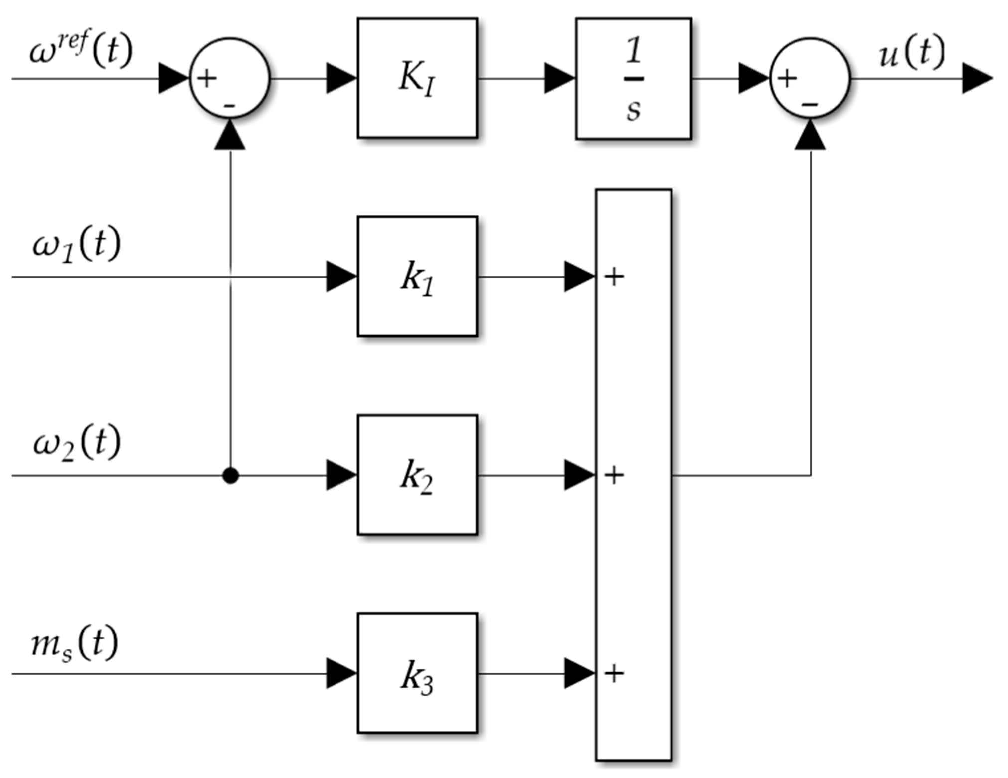
Utilising SFC in two-mass drives is a prevalent conventional solution, as this method allows for the analytical placements of all the poles of the system. It is important to note that the arbitrary determination of the poles requires that the system is fully controllable, and the values of all the required state variables are known, either through measurement or estimation. The proposed controller structure is presented in Figure 3. It comprises feedback loops from both the speed of the motor and the load, as well as the torsional torque:

The determination of controller parameters in state-space is commonly carried out using the classical pole placement method, utilising the characteristic equation of the system. For the cascade speed and the torque control of a two-mass system described by (4) and shown in Figure 2, assuming the torque control loop is optimised to $G_m\left(s\right)=1$, the system transfer function can be expressed as follows:

$$G_{{\omega }_2}\left(s\right)={\displaystyle \frac{{\omega }_2}{{\omega }^{ref}}} ={\displaystyle \frac{K_I}{s^4{T}_1{T}_2{T}_c+s^3{k}_1{T}_2{T}_c+s^2\left(k_2{T}_2+T_1+T_2\right)+s\left(k_1+k_3\right)+K_I}} ,$$

(5)

where $K_I$, $k_1$, $k_2$, and $k_3$—the gain coefficients of the controller.

The characteristic equation of the system is then compared to a reference polynomial equation. Given that the system is fourth order, the characteristic Equation (5) must be equivalent to the following:

$$s^4+s^3\left(4{\xi }_r{\omega }_r\right)+s^2\left(2{{\omega }_r}^2+4{{{{\xi }_r}^2\omega }_r}^2\right)+s\left(4{\xi }_r{{\omega }_r}^3\right)+{{\omega }_r}^4=0,$$

(6)

where ${\xi }_r$—damping coefficient; ${\omega }_r$—resonant frequency.

Through calculations, the following analytical equations for the parameters of SFC are obtained:

$$K_I=T_1{T}_2{T}_c{{\omega }_r}^4,$$

(7)

$$k_1=4T_1{\xi }_r{\omega }_r,$$

(8)

$$k_2=k_1{T}_1{T}_2{{\omega }_r}^2-k_1,$$

(9)

$$k_3=T_1{T}_c\left(2{{\omega }_r}^2+4{{{{\xi }_r}^2\omega }_r}^2-{\displaystyle \frac{1}{T_1{T}_c}}-{\displaystyle \frac{1}{T_2{T}_c}}\right).$$

(10)

3.2. Analytical Model Predictive Control (aMPC)

Consider the following linear discrete form of the state-space equations of the object:

$$\left\{\begin{array}{c}x\left(k+1\right)=\mathit{A}x\left(k\right)+\mathit{B}u\left(k\right)\\ y\left(k\right)=\mathit{C}x\left(k\right)\end{array}\right.,$$

(11)

where $x$—state vector of dimension $n_x$; $u$—input vector of dimension $n_u$; $y$—the measured output vector of dimension $n_y$; and $\mathit{A}$, $\mathit{B}$, and $\mathit{C}$—control system matrices.

The predictive algorithm, utilising the mathematical model of the object at the time $k$, calculates the values of controlled variables at future time $k+p$ (denoted as $p|k$) $y(k+p|k)$ up to the range of predicted future signal samples—termed the prediction horizon $N(p=\mathrm{1,2},\dots ,N)$—and the range of future control signals—termed the control horizon $N_u(p=\mathrm{1,2},\dots ,N_u)<N$. The values of $N$ and $N_u$ are pivotal design parameters of the MPC controller and dictate its performance.

As the current input vector $u\left(k\right|k)$ consists of the previous input signal $u(k-1)$ and increment $\Delta u\left(k\right|k)$, through a recursive process the following matrices for time $p=\mathrm{1,2},\dots ,N$ may be constructed:

$${\mathit{X}}^{pred}\left(k\right)=\left[\begin{array}{c}x\left(k+1|k\right)\\ x\left(k+2|k\right)\\ ⋮\\ x\left(k+N|k\right)\end{array}\right],$$

(12)

$$\Delta \mathit{U}\left(k\right)=\left[\begin{array}{c}\Delta u\left(k|k\right)\\ \Delta u\left(k+1|k\right)\\ ⋮\\ \Delta u\left(k+N_u-1|k\right)\end{array}\right].$$

(13)

The matrix form of the first state equation, as presented in (11), is as follows:

$${\mathit{X}}^{pred}\left(k\right)=\tilde{\mathit{A}}x\left(k\right)+\tilde{\mathit{B}}u\left(k-1\right)+\mathit{P}\Delta \mathit{U}\left(k\right),$$

(14)

where

$$\tilde{\mathit{A}}=\left[\begin{array}{c}\begin{array}{c}\mathit{A}\\ {\mathit{A}}^2\\ ⋮\\ {\mathit{A}}^{N_u}\end{array}\\ {\mathit{A}}^{N_u+1}\\ ⋮\\ {\mathit{A}}^N\end{array}\right], \tilde{\mathit{B}}=\left[\begin{array}{c}\begin{array}{c}\mathit{B}\\ \left(\mathit{A}+\mathit{I}\right)\mathit{B}\\ ⋮\\ \left({\mathit{A}}^{N_u-1}+\dots +\mathit{A}+\mathit{I}\right)\mathit{B}\end{array}\\ \left({\mathit{A}}^{N_u}+\dots +\mathit{A}+\mathit{I}\right)B\\ ⋮\\ \left({\mathit{A}}^{N-1}+\dots +\mathit{A}+\mathit{I}\right)B\end{array}\right],$$

(15)

$$\mathit{P}=\left[\begin{array}{ccc}\mathit{B}& \dots & 0\\ \left(\mathit{A}+\mathit{I}\right)\mathit{B}& \dots & 0\\ ⋮& \ddots & ⋮\\ \left({\mathit{A}}^{N_u-1}+\dots +\mathit{A}+\mathit{I}\right)\mathit{B}& \dots & \mathit{B}\\ \left({\mathit{A}}^{N_u}+\dots +\mathit{A}+\mathit{I}\right)\mathit{B}& \dots & \left(\mathit{A}+\mathit{I}\right)\mathit{B}\\ ⋮& \ddots & ⋮\\ \left({\mathit{A}}^{N-1}+\dots +\mathit{A}+\mathit{I}\right)\mathit{B}& \dots & \left({\mathit{A}}^{N-N_u}+\dots +\mathit{A}+\mathit{I}\right)\mathit{B}\end{array}\right].$$

(16)

With the use of (14), the second state equation can be expressed as follows:

$$\begin{array}{c}{\mathit{Y}}^{pred}\left(k\right)=\tilde{\mathit{C}}{\mathit{X}}^{pred}\left(k\right)=\tilde{\mathit{C}}\left(\tilde{\mathit{A}}x\left(k\right)+\tilde{\mathit{B}}u\left(k-1\right)+\mathit{P}\Delta \mathit{U}\left(k\right)\right)=\\ \tilde{\mathit{C}}\left(\tilde{\mathit{A}}x\left(k\right)+\tilde{\mathit{B}}u\left(k-1\right)\right)+\tilde{\mathit{C}}\mathit{P}\Delta \mathit{U}\left(k\right)={\mathit{Y}}_0\left(k\right)+\Delta \mathit{Y}\left(k\right),\end{array}$$

(17)

where $\tilde{\mathit{C}}$—a diagonal output matrix with element $\mathit{C}$ and the dimension $N·n_y\times N·n_x$.

The final form of the output state equation consists of two components: ${\mathit{Y}}_0\left(k\right)$, which is related to the current object state and previously applied control; and $\Delta \mathit{Y}\left(k\right)$, which corresponds to the newly imposed control for predicted output trajectory. It can be seen that the numerical complexity of this algorithm is linked to the size of the matrix $\mathit{C}$ (length of vectors $n_x$, $n_y$) and the length of the prediction horizon $N$.

The determination of control values in prediction algorithms is achieved through the minimisation of the criteria function $J,$ which indicates the control quality at the prediction horizon. The most common derivation includes the cost of deviations at the predicted output trajectory from the reference and a penalty for the variability of the determined control signals:

$$J\left(k\right)={‖\left({\mathit{Y}}^{ref}\left(k\right)-\mathit{Y}\left(k\right)\right)-\mathit{M}\Delta \mathit{U}\left(k\right)‖}^2+{‖\Delta \mathit{U}\left(k\right)‖}^2,$$

(18)

where $\mathit{M}=\tilde{\mathit{C}}\mathit{P}$—dynamic matrix.

Assuming the strict convexity of the function $J$ and no imposed constraints, the vector of optimal control elements is as follows:

$$\Delta \widehat{\mathit{U}}\left(k\right)=\mathit{K}\left({\mathit{Y}}^{ref}\left(k\right)-\mathit{Y}\left(k\right)\right),$$

(19)

where $\mathit{K}={R\left({\mathit{M}}^T\mathit{M}\right)}^{-1}{\mathit{M}}^T$; $R$—output gain coefficient.

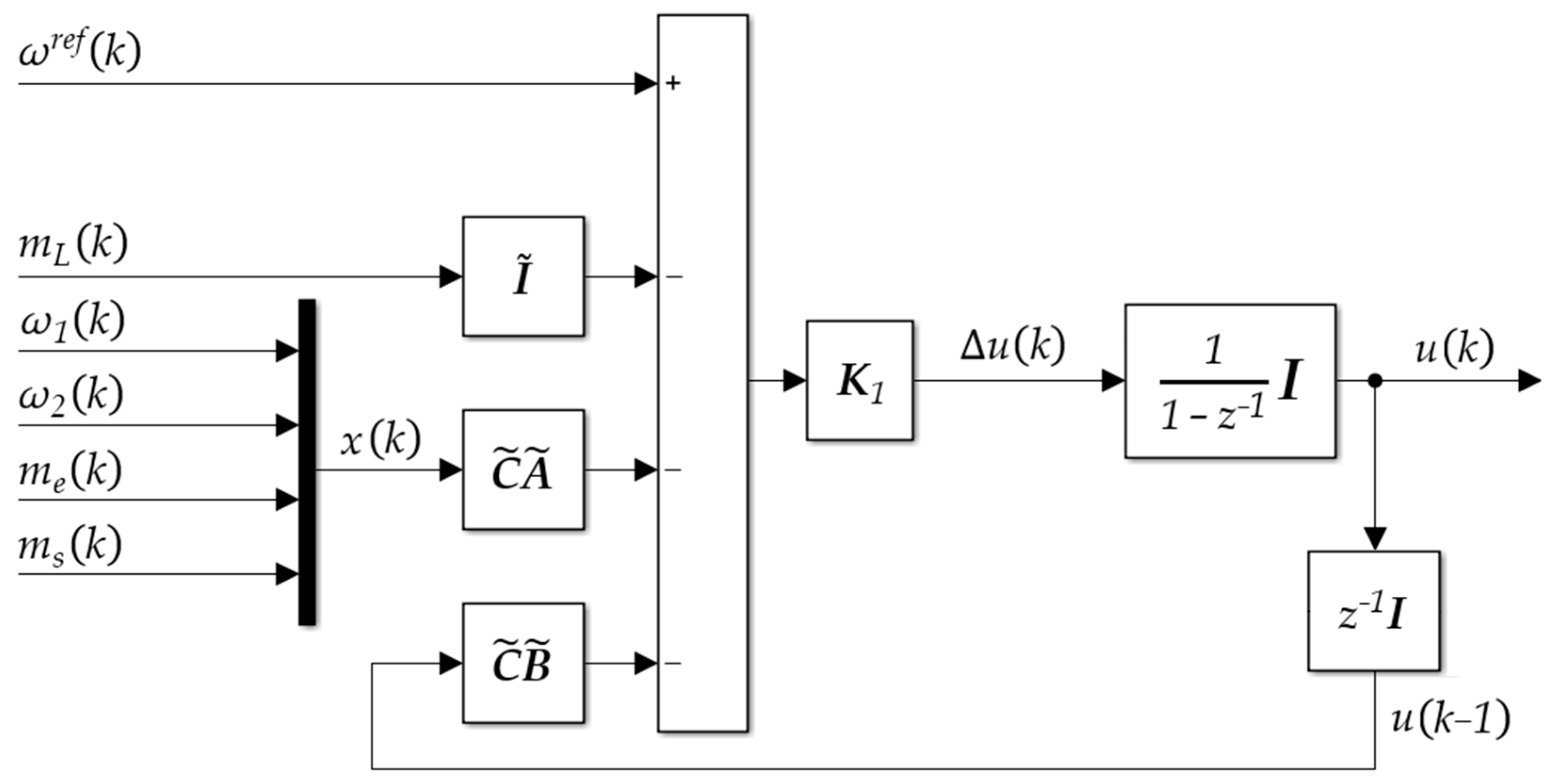
The matrix $\mathit{K}$ represents a least-squares solution and is computed using the dynamic matrix $\mathit{M}$, which encapsulates the system’s response to control inputs over the prediction horizon. As such, $\mathit{K}$ inherently reflects the underlying system dynamics and provides the optimal control signal gains. The inclusion of the scalar gain coefficient $R$ enables the tuning of the control law, determining how strongly the controller reacts to predicted output errors. The algorithm used to calculate the above matrices for the purposes of this study is presented in Appendix A, and the block diagram is shown in Figure 4.

In aMPC, the control signal is derived via a receding-horizon approach. At each subsequent time step $k$, the algorithm determines optimal control increments up to the control horizon length $N_u$, but only the first element $\Delta \widehat{u}\left(k\right)$ is applied to the object:

$$\Delta \widehat{u}\left(k\right)={\mathit{K}}_1\left({\mathit{Y}}^{ref}\left(k\right)-{\mathit{Y}}^0\left(k\right)\right),$$

(20)

where ${\mathit{K}}_1$—a submatrix consisting of the first row of matrix $\mathit{K}$.

Ultimately, it can be observed that the proposed aMPC is linear and its control law may be defined as follows:

$$\Delta \widehat{u}\left(k\right)={\mathit{K}}_1\left({\mathit{Y}}^{ref}\left(k\right)-\mathit{Y}\left(k\right)-\mathit{M}\Delta \mathit{U}\left(k\right)\right)$$

(21)

4. Control Structure

4.1. Proposed Cascade Control Structure

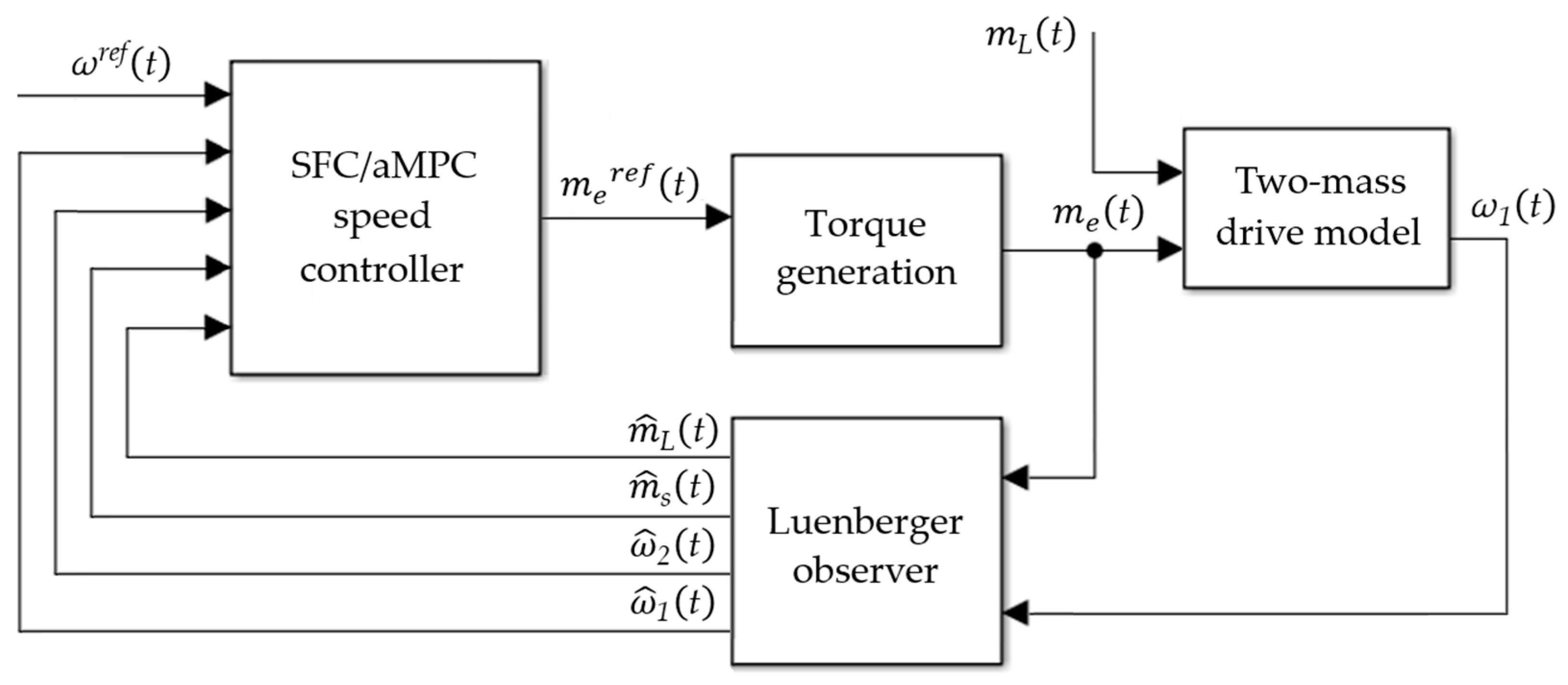
The general speed control structure proposed for this study is presented in Figure 5.

Firstly, the two-mass block represents the state-space model of the considered drive, as previously shown in Figure 2. The inner torque control loop comprises the power converter and a torque (current) controller with its respective sensor. Given the importance of dynamic and accurate torque control, as well as the multitude of optimisation approaches, a correctly tuned inner loop may be simplified to a single first order term, dependent on a small time constant [9,11]. The outer loop, acting as the master in the cascade control structure, consists of the selected speed controller with its respective sensors. Finally, external constraint ${m_{\mathrm{e}}}^{\max }=\pm 2m_{\mathrm{N}}$ (where $m_N$ is the nominal torque) is imposed on the controller output through a saturation block.

As both of the considered controllers rely on the mathematical model of the object, feedback loops of the state variables are required. In industrial applications, a trend towards sensorless drivers has emerged, involving the measurement of only the motor speed ${\omega }_1$ and electromagnetic torque $m_e$ and the estimation of the other state variables. It is worth noting that although the motor speed ${\omega }_1$ is measured, its estimate is utilised in the control structure. This approach serves to avert the conflation of measured and estimated speed signals, due to the potential delay introduced by the observer.

While numerous interesting solutions have been presented in the literature, it is not the primary focus of this particular study, and therefore a classical Luenberger observer has been implemented.

4.2. Control Quality Evaluation

In order to evaluate the control quality of a designed structure, it is advisable to specify and analyse the value of a selected performance function. The Integral Time Absolute Error (ITAE) is a common choice; however in two-mass drives, it is not fully representative of the dynamics of the system because of the speed difference on the motor and the load side. To address this issue, an expanded performance function $f$ is proposed—consisting of the integral criteria ITAE of both the motor and the load speed, as well as the sum of absolute speed differences and the mean absolute error of electromagnetic torque derivatives. These indicators are paired with respective weight factors. While the values presented below have been defined arbitrarily by the authors based on the results of the conducted tests, they may be modified according to individual needs:

$$f =0.2·ITAE\left({\omega }_1\left(t\right)\right)+0.7·ITAE\left({\omega }_2\left(t\right)\right)+0.05·\sum _{i=1}^n\left|{\omega }_2\left(t\right)-{\omega }_1\left(t\right)\right|+0.05·{\displaystyle \frac{1}{n}}\sum _{i=1}^n{\displaystyle \frac{d{m}_e\left(t\right)}{dt}}$$

(22)

Within the multi-objective performance function, the two ITAE components reflect how accurately the respective machines follow the reference speed trajectory. The speed difference caused by the elastic coupling is further represented in the third term (speed concurrency). Lastly, a component related to torque control is introduced. Although not directly related to drive speed, it serves to evaluate the smoothness of torque control by penalising high-frequency variations in the applied electromagnetic torque. During dynamic operation, rapid fluctuations in torque may be undesirable, as they can place mechanical stress on the drive components, potentially leading to wear or damage.

As the performance of the proposed speed controllers depends on multiple parameters simultaneously, adjusting their parameters may be problematic without conducting a prior analysis. However, the tuning process can be automated using pattern search or genetic algorithms (GAs). For this study, MATLAB’s built-in GA function was applied, with the presented performance function $f$ (22) serving as the minimised objective function.

5. Simulation Study

Preliminary simulation tests were conducted in MATLAB/Simulink R2023b, assuming the nominal parameters of the drive as $T_1=0.203 \mathrm{s}$, $T_2=0.285 \mathrm{s}$, and $T_c=0.0012 \mathrm{s}$. The state-space object model (4) was discretised using a first-order Taylor approximation with a sampling time of $T_s=0.5 \mathrm{m}\mathrm{s}$, while the Simulink model operated with a sampling time of $T_{sim}=0.01 \mathrm{m}\mathrm{s}$. The optimised torque control loop was represented as a first-order term with time constant $T_{m_e}=0.2 \mathrm{m}\mathrm{s}$. For the state variable estimation, a Luenberger observer with a damping coefficient of ${\xi }_L=1$ and a frequency of ${\omega }_L=160{\mathrm{s}}^{-1}$ was employed.

5.1. Analytical Model Predictive Control (aMPC) Tests

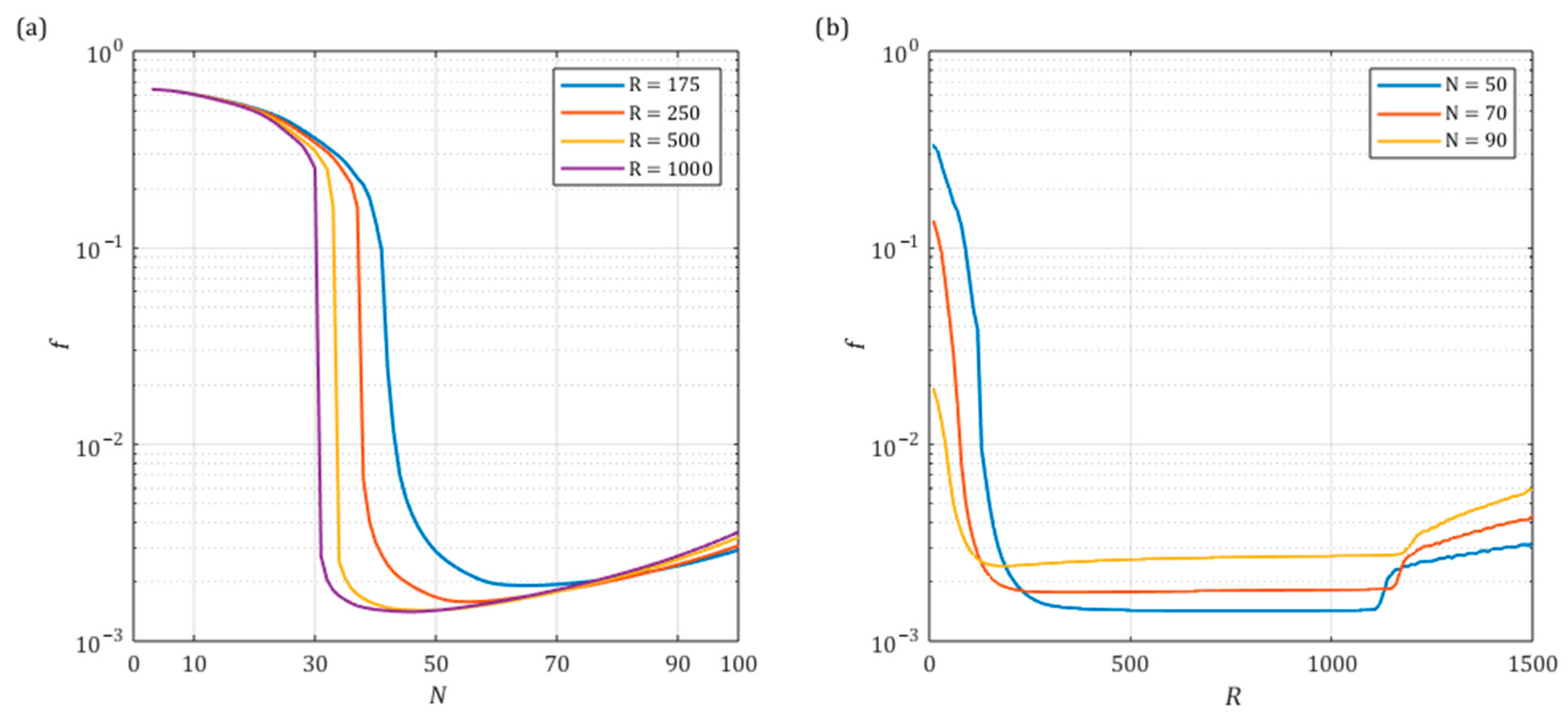
Firstly, a series of tests were conducted to assess the impact of the aMPC parameters on the value of the performance function $f$. The results of this analysis are presented in Figure 6.

First and foremost, it can be seen that the prediction horizon $N$ has a substantial influence on the performance of the drive. Inadequate lengths of the prediction horizon may result in the manifestation of oscillatory behaviour or even a loss of stability.

Of significance, the prediction horizon $N$ defines the number of future time steps over which the prediction process occurs. Consequently, it is inherently linked to the sampling time of the controller $T_s$. The selection of these two parameters requires careful consideration, as the determined predicted time window must exceed the maximal time constant of the object, in this case $T_2$. This is the point at which a sharp decrease in the performance function value can be observed. Further extending the prediction horizon has little effect on the performance function yet increases the computational complexity of the controller and is, therefore, inadvisable.

As demonstrated in Figure 6b, initially increasing the value of gain coefficient $R$ enables the reduction of the function $f$ through amplifying the control signal and thus improving system dynamics. Beyond a certain point, depending on the length of the prediction horizon $N$, progress in minimising the performance function halts. Further increases in the value of $R$ appear to have little effect on the control quality. However, in the case of very high gains, a marked increase of $f$ can be observed. Note that the controller output is externally constrained, and with larger and larger values of $R$, the control signal approaches its limit more easily. Eventually, the controller starts to perpetually operate in saturation. Therefore, excessive values of $R$ are not recommended either.

Increasing the control horizon $N_u$ results in a substantial increase in the computational complexity of the controller, as for every sample, the minimisation process of the criteria function $J$(18) must be repeated. In the case of the analysed system, increasing $N_u$ beyond one sample already resulted in a significant deterioration of the quality of control and a loss of stability. In light of the above observations, the value of $N_u=1$ was adopted for this research.

The simulation results for the drive state variables are presented in Figure 7. The reference speed signal in the system was a step function to ${\omega }^{ref}=0.25$ and ${\omega }^{ref}=0.1$. Additionally, at time $t=0.5 \mathrm{s}$, nominal load torque was introduced to the system. The parameters of aMPC were tuned through the minimisation of $f$ by MATLAB’s built-in GA.

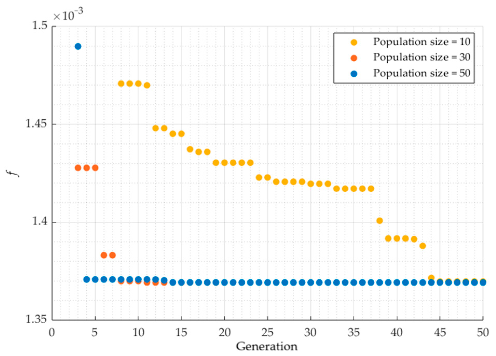
For the optimisation process, a population size of $P=50$ was adopted, and the GA usually converged to the optimal solution within 5–15 generations. It is worth noting that the prediction horizon $N$ is an integer value, and the control horizon is expected to be $N_u=1$. This greatly reduces the search space and simplifies the optimization process, allowing the GA to find the optimal solution very quickly.

Figure 7 illustrates the progression of the optimisation process for different population sizes—namely $P=10, P=30$, and $P=50$. In all three cases, the GA converged to the same final result, although in a different number of generations. This further confirms the validity of the controller parameters adopted for further studies, which were as follows: $N=48, N_u=1, R=830$.

As can be concluded from the results, the proposed structure ensures the correct operation of the system and is capable of actively suppressing the effects of torsional vibrations on the load speed. A noteworthy characteristic of the control of two-mass drives is the necessity to compensate for the elasticity of the shaft by momentarily forcing reverse electromagnetic torque during dynamic processes. This effect is most evidently seen during start-up, at around $t=0.05 \mathrm{s}$.

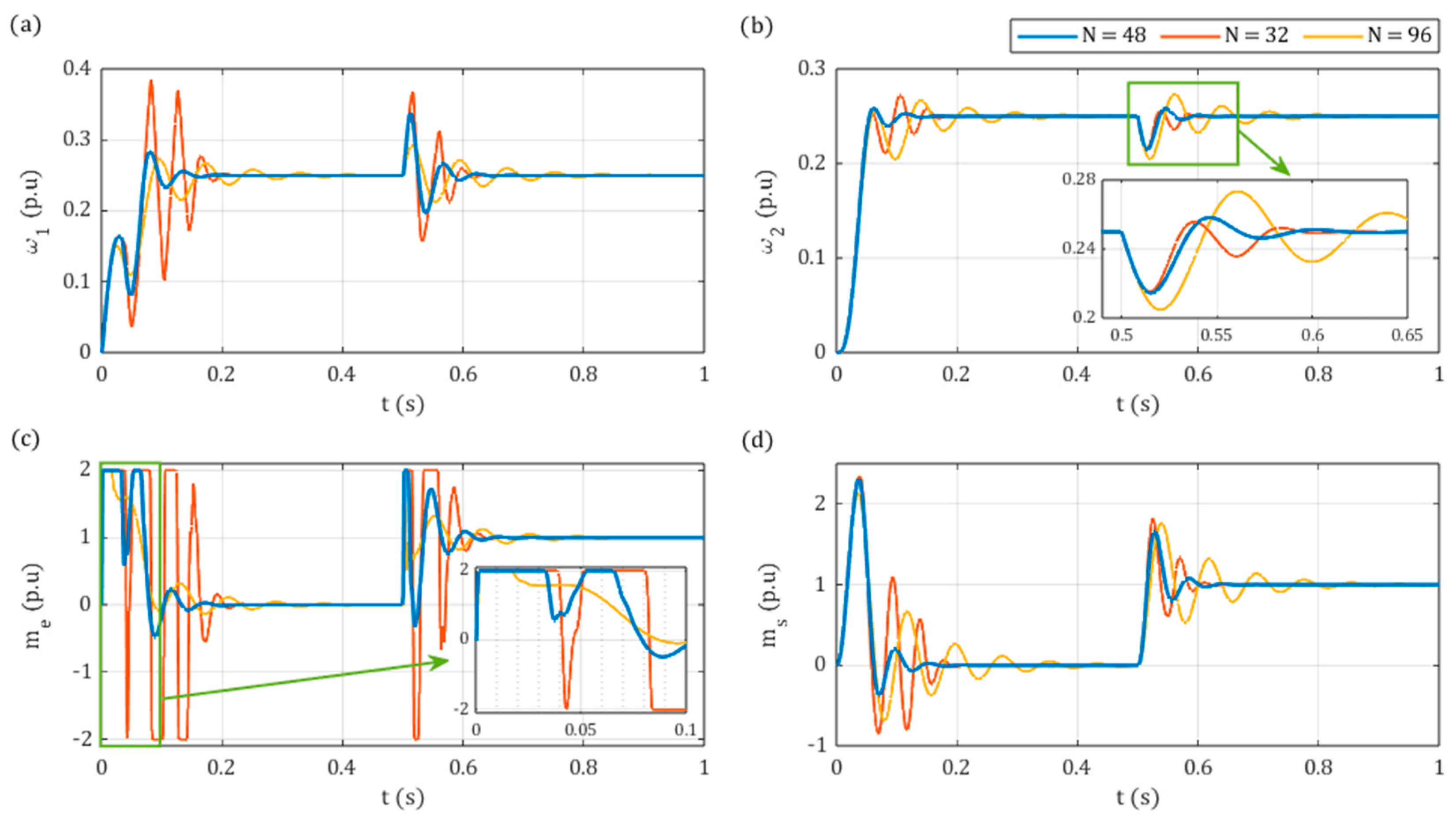
In addition to the transients obtained with the use of the GA, the results for two additional lengths of $N$ are presented; notably, the lowest value for which the system is stable ($N=32$) and twice the original length ($N=96$). As previously mentioned, with the shorter prediction horizon $N=32$, the oscillatory character of the motor speed is enhanced by up to 45% during load application (Figure 8a), which can also be reflected in the load speed (Figure 8b). In contrast, a significant increase of $N=96$ facilitates smoother torque control (Figure 8c) at the expense of significantly longer transition processes, in this case almost tripling its duration.

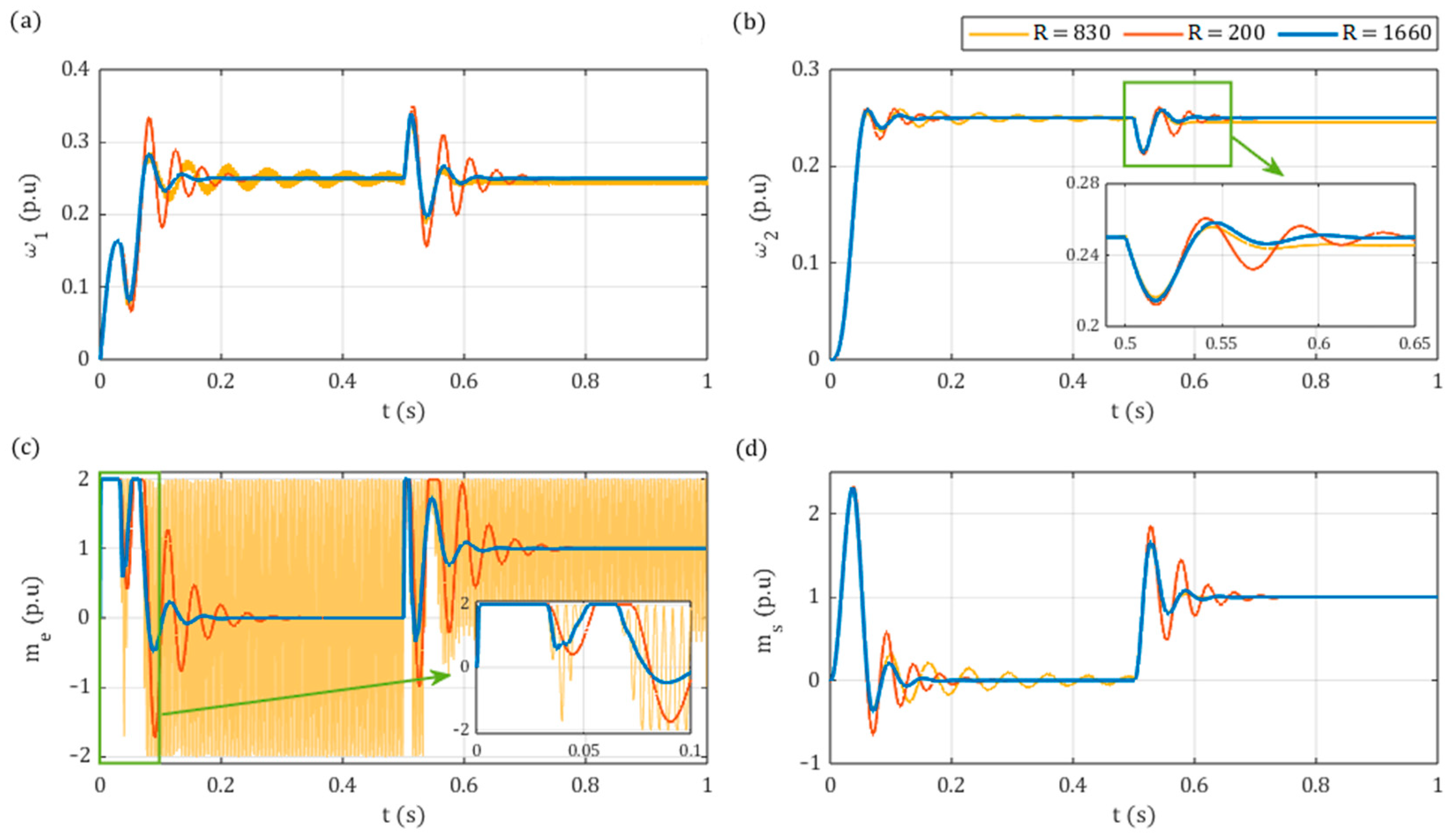
The simulation results depending on the gain coefficient $R$ are presented in Figure 9. The parameters have been selected to outline the effects that occur in the instances of both too low ($R=200$) and too high ($R=1660$) gain values, as demonstrated in Figure 6b. For very low values of $R$, the system dynamics are insufficient, leading to approximately twice-as-strong oscillations of the torque and, consequently, an almost 50% stronger motor speed. A further decrease causes increasingly volatile torque oscillations and ultimately the loss of stability. On the opposite end, extremely high gain values cause the controller to operate in saturation, resulting in continuous fluctuations up to the maximal torque (Figure 9c). In addition to the oscillations in the speed of both machines, a 1.6% steady-state error in the load speed can be observed (Figure 9b).

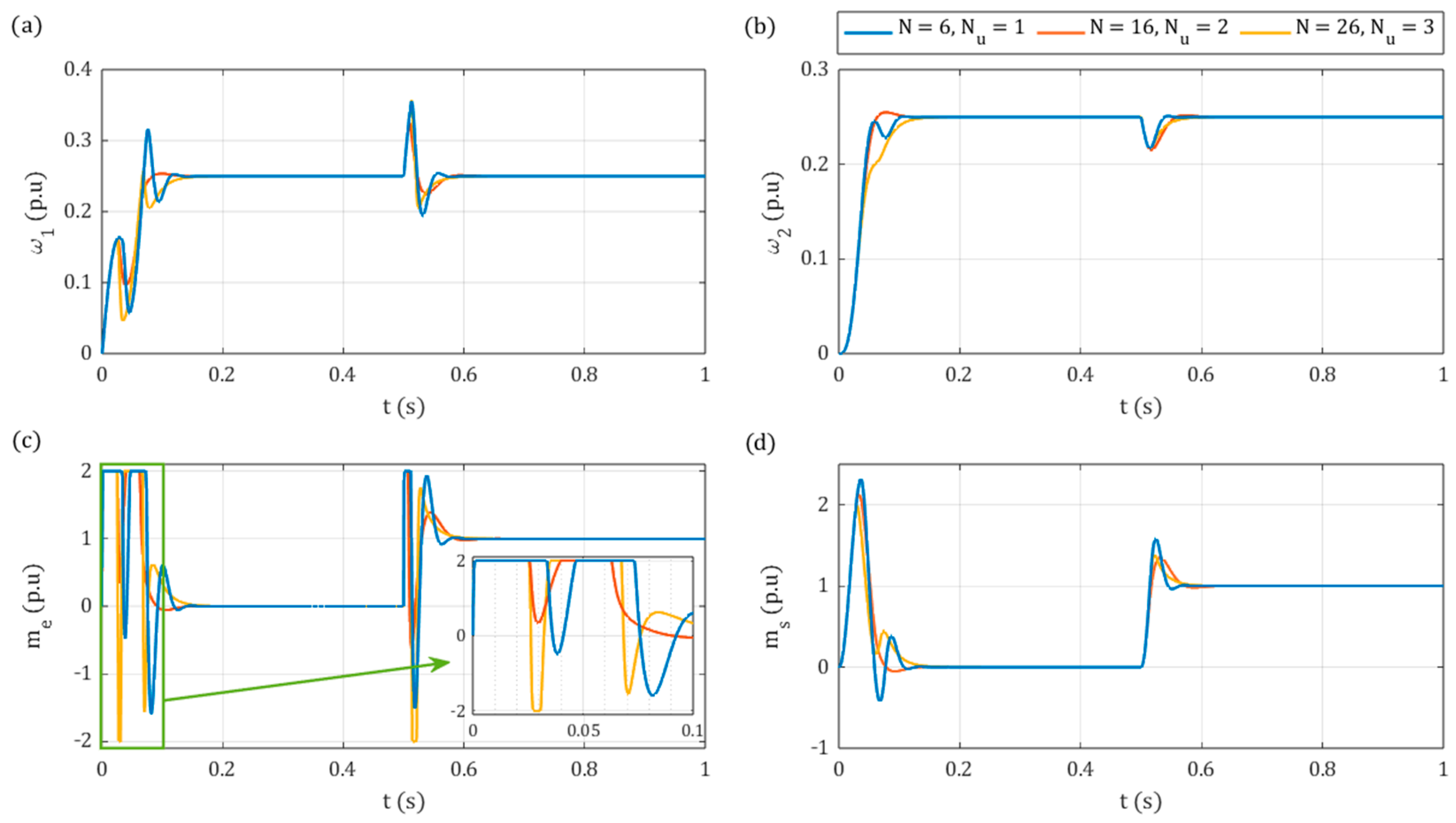
Lastly, the influence of the length of the control horizon $N_u$ was analysed. It is evident from (13) that increasing the control horizon results in a substantial increase in the computational complexity of the controller, as for each additional sample, the minimisation process of the criteria function $J$ (18) must be repeated. In the case of the analysed system, increasing $N_u$ beyond one sample already resulted in a significant deterioration of the quality of control and a loss of stability.

However, with more lenient sampling times, it is possible to extend the control horizon, as shown in Figure 10 for $T_s=3 \mathrm{m}\mathrm{s}$. The primary benefit of extending the control horizon is the potential of acquiring more precise control during dynamic processes, which enables smoother motor speed (Figure 10a) and torsional torque (Figure 10c) transients during start-up. However, the determination of the control signal becomes a more complex process, and the response to the load torque is notably slower.

It is noteworthy that with a change in $N_u$, the length of the prediction horizon $N$ also must be adjusted to be sufficiently longer, which further complicates the tuning process. In light of these observations, the value of $N_u=1$ was adopted for further study.

5.2. Comparative Study

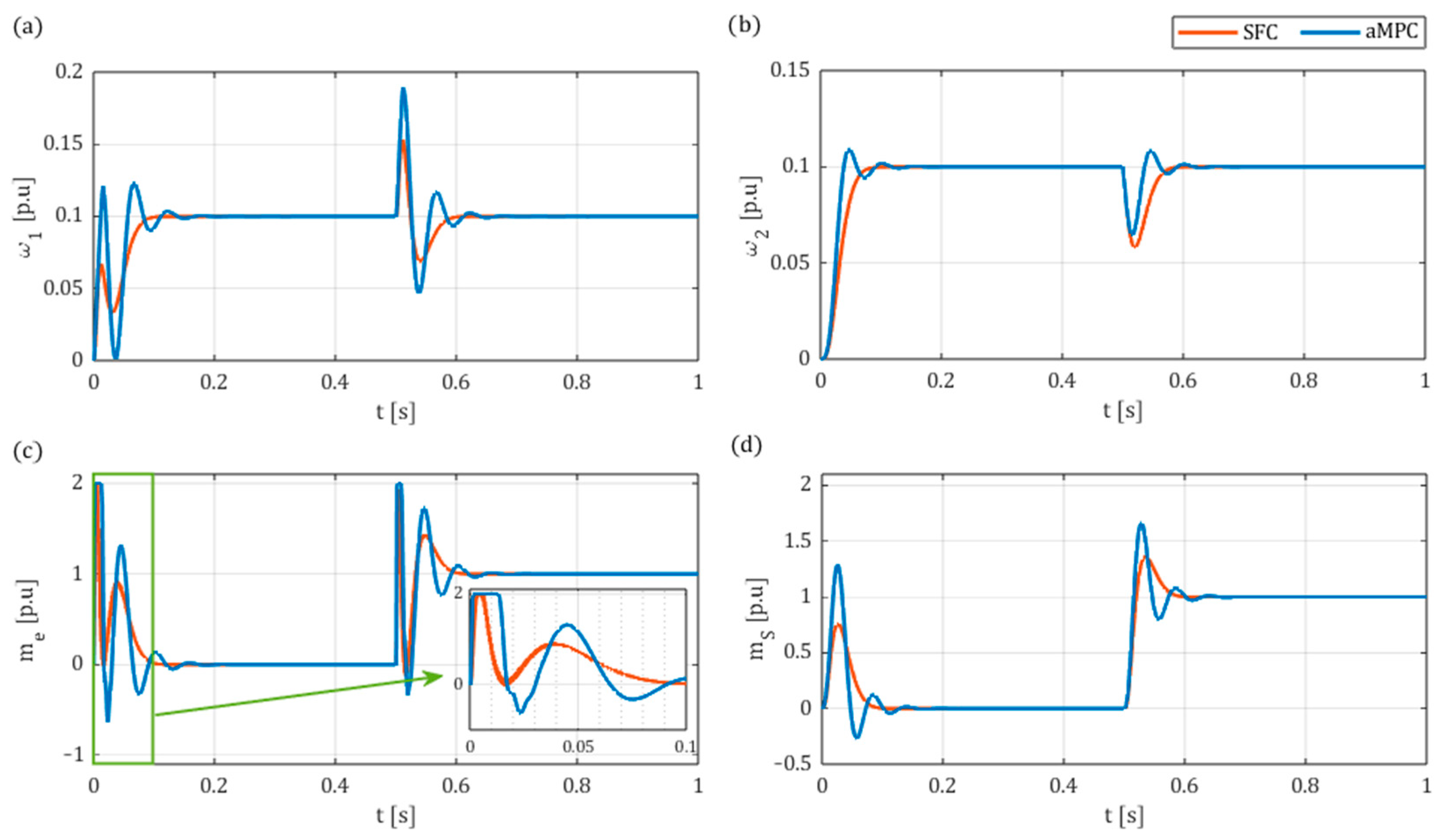
For comparison purposes, firstly the SFC model was tuned utilising the same GA method. The objective of the tuning process was to replicate the dynamics obtained for the aMPC-based system. Below in Figure 11 and Figure 12 are the simulation results for the obtained SFC parameters: ${\xi }_r=0.84$ and ${\omega }_r=110 {\mathrm{s}}^{-1}$. As can be seen, both of the considered controllers are able to successfully reduce the effect of the torsional vibrations on the dynamics of the system. The step responses of the load speed are characterised by a virtually equal rate of increase. Additionally, the performance function of both control systems is nearly equal, at $f$ = 1.4209 × 10⁻³ for SFC and $f$ = 1.4197 × 10⁻³ for aMPC. Still, slightly smoother torque transients and a shorter transition process after introducing the load torque can be observed for aMPC.

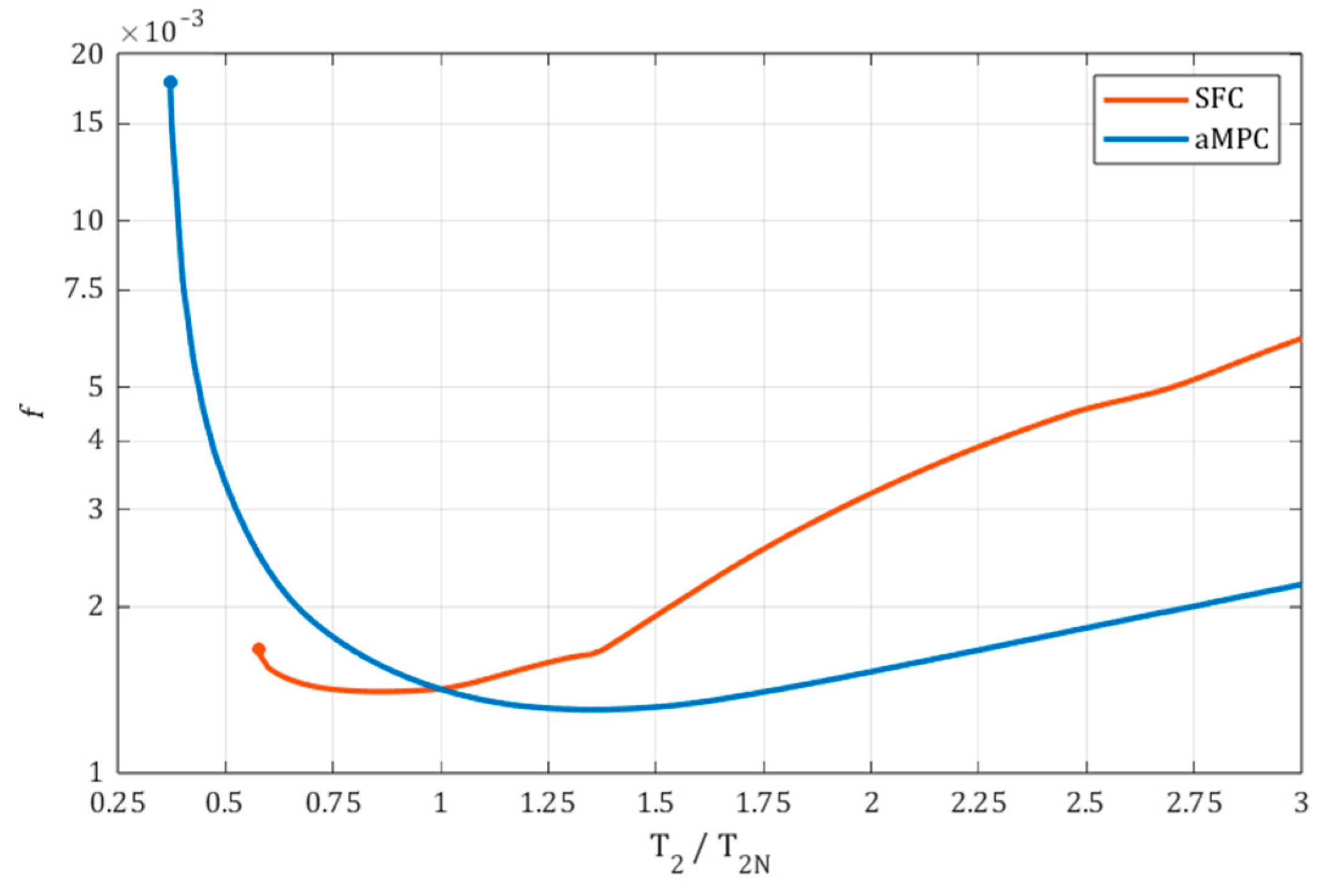
As mentioned in the introduction, the load moment of inertia, represented by its time constant $T_2$, may be subject to changes during operation due to the nature of the load machine. Therefore, the effect of this parameter change was investigated to assess the robustness of both proposed solutions. This was done by modifying the value of $T_2$ in the Simulink model, while both controllers remained tuned for $T_2=T_{2N}=0.285 \mathrm{s}$.

A comparison of control structure performances through the value of $f$ is presented in Figure 13. The examined range of $T_2$ was assumed from 0.3 to triple of the nominal value. The findings indicate that both proposed control systems respond in different ways to alterations in the parameters of the load machine. For values of the $T_2/T_{2N}$ ratio greater than one, aMPC demonstrates clearly better robustness. At $T_2/T_{2N}=2$, the performance function for SFC is more than twice as high, at $f$ = 3.3084 × 10⁻³ versus $f$ = 1.5271 × 10⁻³ for aMPC. On the other hand, SFC provides slightly better results as the ratio is decreased below one, demonstrating, notably, around a 25% lower performance function value for $T_2/T_{2N}=0.75.$ However, at around $T_2/T_{2N}\approx 0.55$, the SFC-based structure becomes unstable, while the aMPC model retained stability until around $T_2/T_{2N}\approx 0.37$.

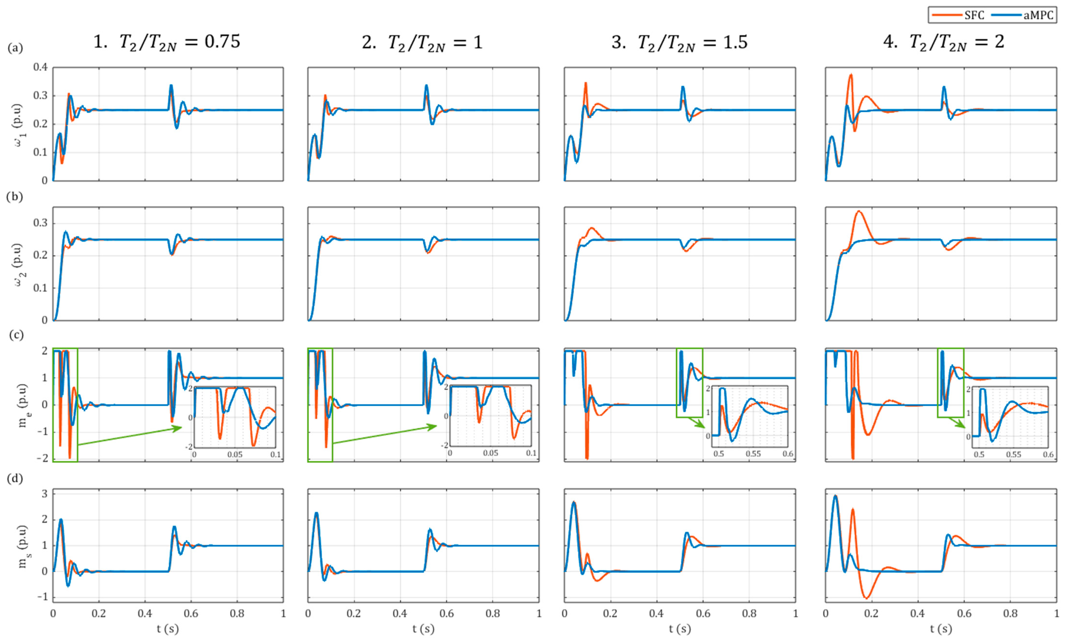
Finally, the comparative simulation results of the step responses of both control structures for different values of $T_2$ are showcased in Figure 14 (as SFC became unstable for half of the nominal $T_2$, the results have not been included). The examination of the obtained transients confirms the conclusions drawn above. With increasingly higher time constants $T_2$, SFC becomes significantly more oscillatory, resulting in overshoots of the load speed upwards of 48% in the case of $T_2/T_{2N}=2$. Additionally, a longer settling time, as well as more pronounced torsional torque oscillations, can be observed.

In relation, aMPC appears to only be minimally affected. Even when the time constant $T_2$ approaches twice its original value, only a 20% increase in the performance value function was noted. Nevertheless, SFC ensures a less oscillatory character of the motor and the load speed in the case of $T_2/T_{2N}=0.75$; however, this is at the expense of more abrupt torque variations.

The superior robustness of aMPC in cases of the underestimation of $T_2$ is directly attributable to the predictive nature of the control strategy. This is particularly evident in the responses shown in Figure 14 for $T_2/T_{2N}=2$, where both controllers demonstrate similar dynamics up to the point of reaching the reference value at around $t=0.1 \mathrm{s}$. However, aMPC—by anticipating future system behaviour—reduces the control signal earlier, resulting in a significantly lower overshoot. Conversely, the diminished performance control of aMPC for $T_2/T_{2N}<1$ stems from its attempt to maintain the dynamics corresponding to nominal parameters. In contrast, SFC responds more rapidly due to the decreased time constant, but also loses stability much sooner.

6. Experimental Results

6.1. Laboratory Setup

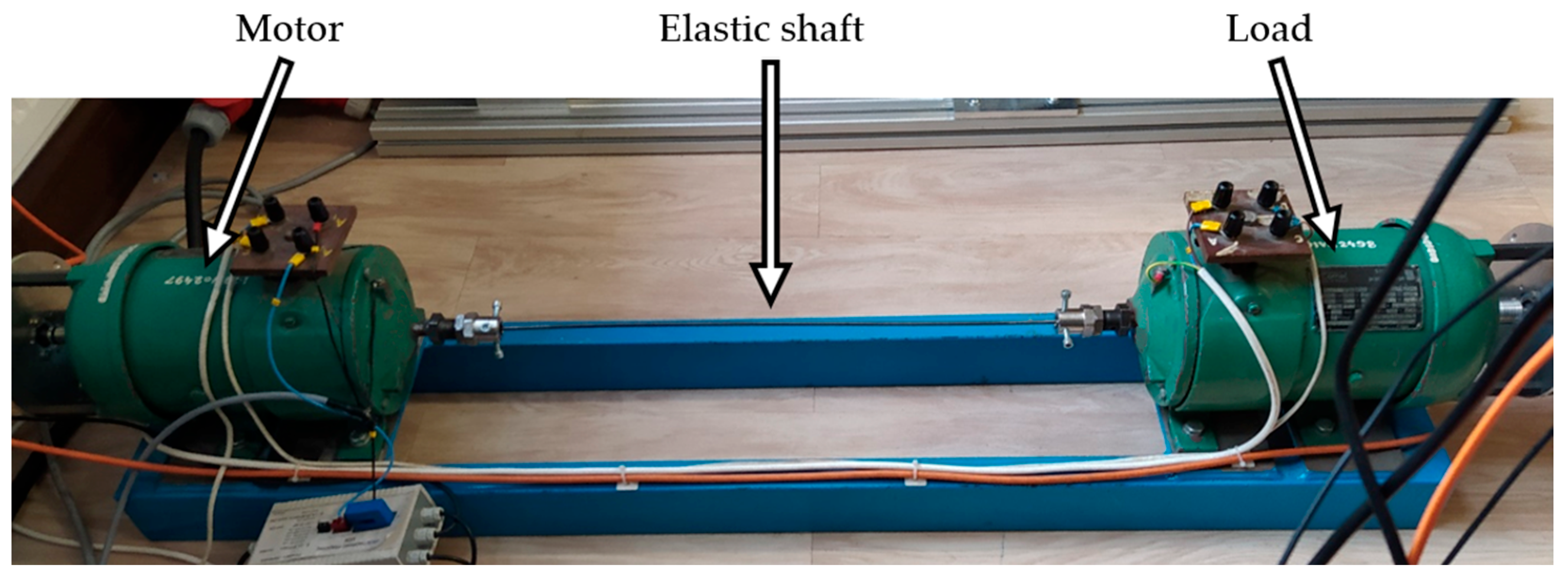
Following the execution of simulation tests, the presented control structures were subjected to experimental verification. The laboratory stand presented in Figure 15 incorporates two 500 W DC motors; one functions as the drive motor and the other serves as a generator to generate load torque. The machines in this system are connected by interchangeable elastic steel shafts. In this particular case, the shaft was characterised by length $l=600 \mathrm{m}\mathrm{m}$, diameter $d=5 \mathrm{m}\mathrm{m}$, and time constant $T_c=0.0012 \mathrm{s}$. The technical specifications of the utilised PZBb 22b DC motor are presented in full in

Table 1. Parameters of the DC motor.

Nominal Parameter	Notation	Value
Power	$P_N$	500 W
Voltage	$U_N$	220 V
Armature current	$I_{aN}$	3.15 A
Field current	$I_{fN}$	0.254 A
Speed	$n_N$	1450 rpm
Moment of inertia	$J$	0.044 $\mathrm{k}\mathrm{g}{\mathrm{m}}^2$
Armature circuit resistance	$R_t$	8.05 $\mathsf{\Omega }$
Armature circuit inductance	$L_t$	0.8 H
Moment of inertia	$J$	0.044 $\mathrm{k}\mathrm{g}{\mathrm{m}}^2$

:

Figure 16 presents a schematic representation of the laboratory stand. The drive motor is powered by an H-bridge power converter, which is controlled through Pulse Width Modulation (PWM). The speed of both machines is measured by Fritz Kübler GmbH (Villingen-Schwenningen, Germany) 5805 incremental encoders, with resolution of 36,000 pulses per rotation, and the armature current is measured through a LEM (Groß-Gerau, Germany) converter.

The control structures were initially developed in MATLAB/Simulink R2023b and then compiled into C language with the use of Real Time Workshop. Next, they were transferred to a dSpace GmbH (Paderborn, Germany) DS1103 PPC Controller Kit, which is equipped with a DSP signal processor and I/O circuits acting as the interface with the sensors and actuators. The data collection, monitoring, and control of the system were implemented as a virtual control panel in the ControlDesk 3.7.3 environment.

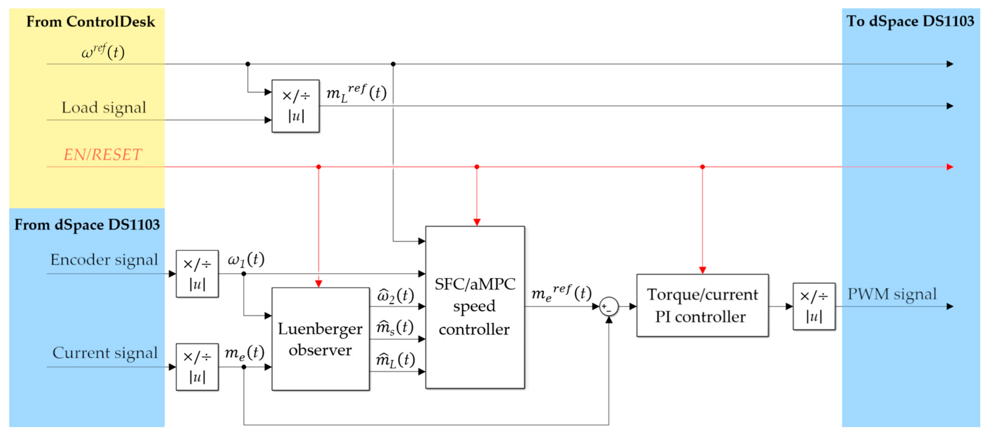
Figure 17 illustrates the control structure within the MATLAB/Simulink environment. Input signals from the dSpace DS1103 card and the virtual control panel are introduced using blocks from the Real-Time Interface (RTI) custom library. Following the scaling and normalisation into the per-unit system, the structure is analogous to that shown in Figure 5. Although the speed of both motors can be measured on the laboratory setup, this is not always feasible under practical implementation conditions. Consequently, the only measured values are the encoder signal and the current signal of the driving motor.

From the control panel, the user is able to set the speed and load torque reference signal, as well as enable or RESET the control structure. The timing of the load torque is synchronised to the reference speed, and load control is achieved through the exciting current of the load motor acting as a generator.

6.2. Results

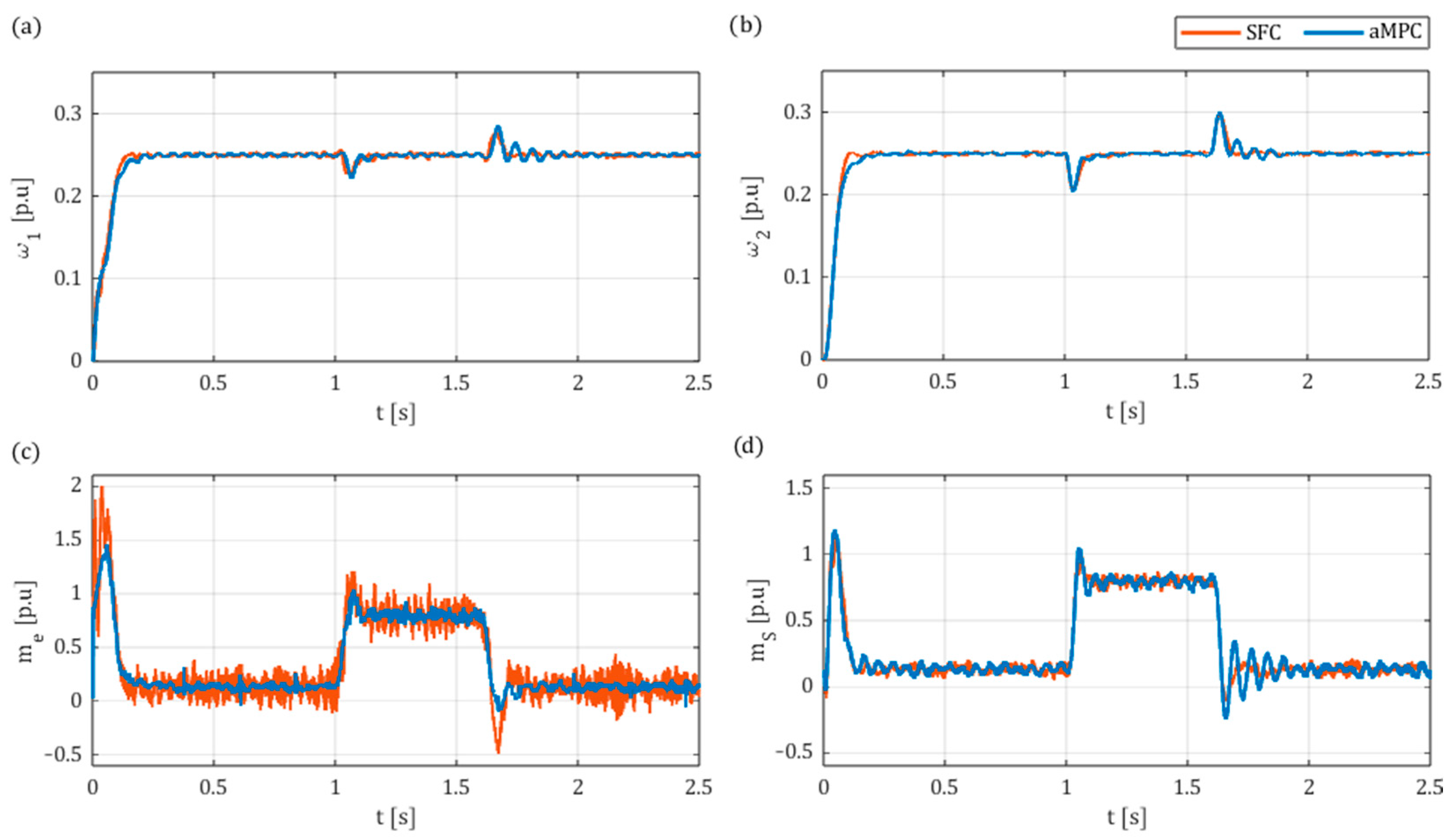
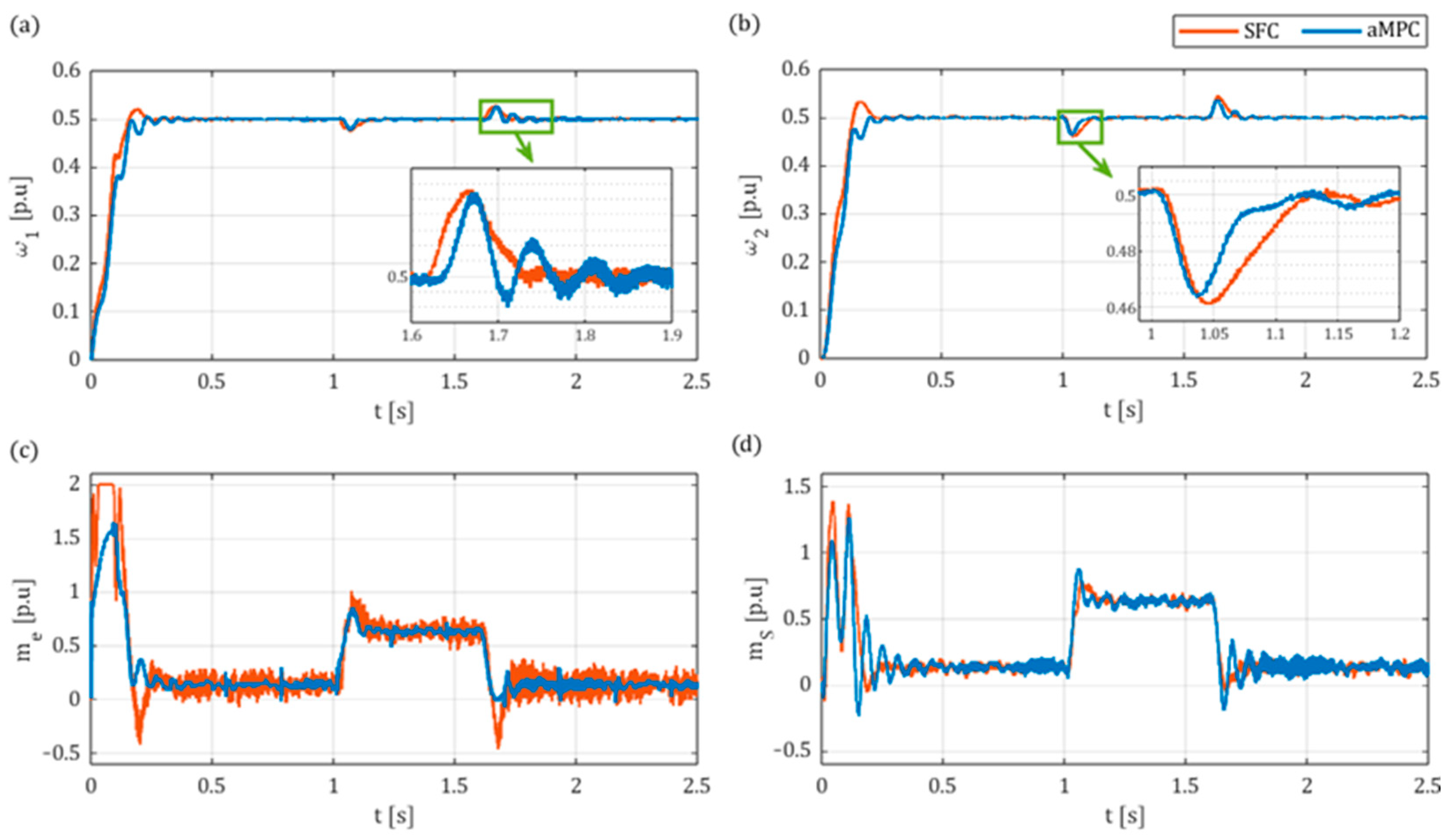
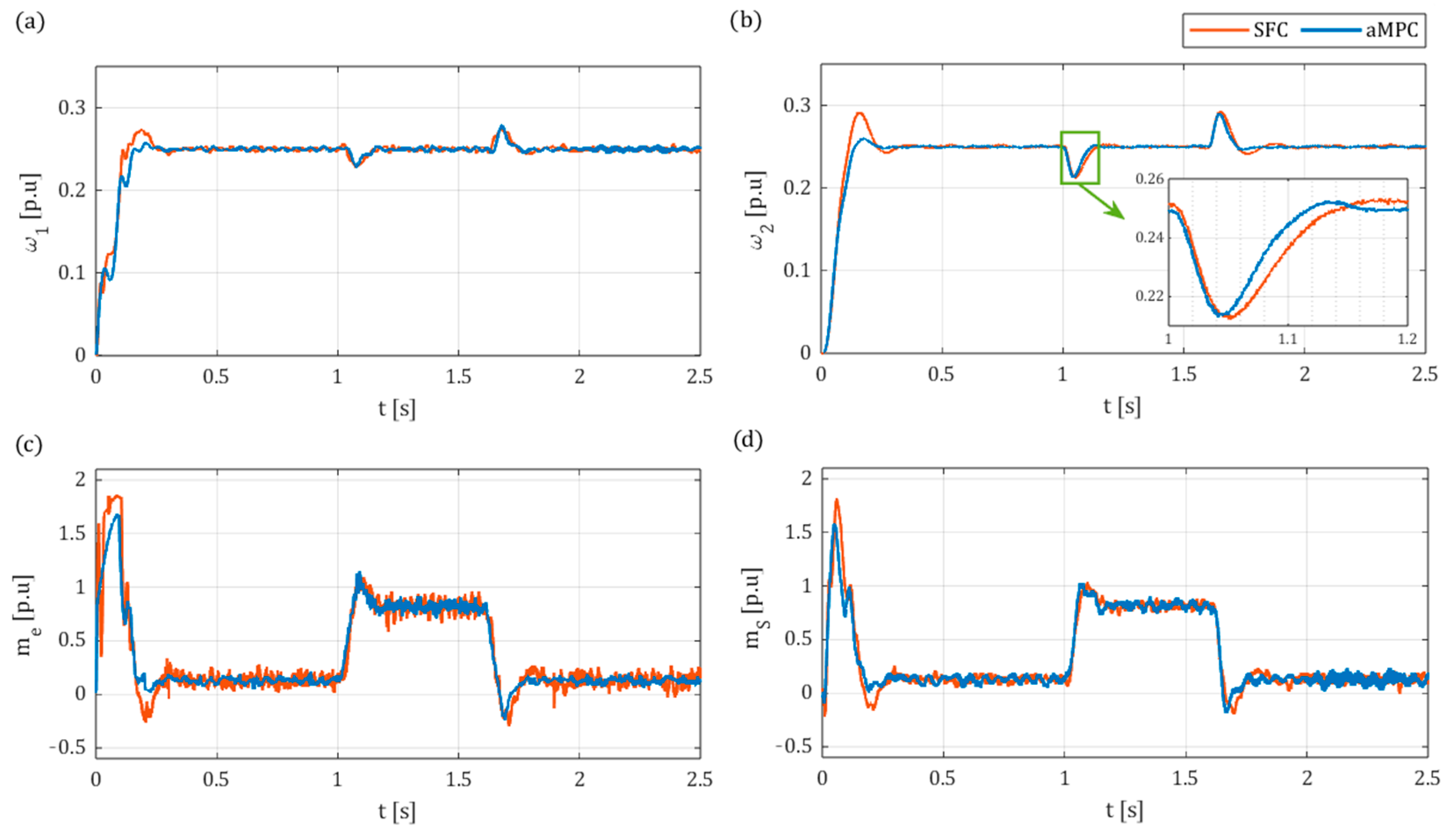
All the experimental tests were conducted on the described laboratory setup, the parameters of which had also previously been utilised for the simulation model. In the laboratory plant, the inner torque (current) loop was operated by a PI controller with coefficient gains of $K_p=0.5$ and $K_i=10$. The sampling time of both control loops and the Simulink model equalled $T_s=T_{sim}=0.5 \mathrm{m}\mathrm{s}$. The experimental step responses to reference speeds of ${\omega }^{ref}=0.25$ and ${\omega }^{ref}=0.5$ were investigated. For these tests, the drive operated under a load torque of between $t=1 \mathrm{s}$ and $t=1.6 \mathrm{s}$. Lastly, the results of sine wave tracking for both control systems are presented.

During the initial phase of experimental tests, it was observed that the implementation of the SFC parameters derived directly from the simulation analysis resulted in the unreliable operation of the system. The high levels of the desired dynamics, in conjunction with unmodelled disturbances—such as measurement noise—resulted in violent torque (current) control. In order to ensure safe and stable experimental operation, it was necessary to reduce the dynamics of SFC. Specifically, its resonance frequency was reduced from ${\omega }_r=110 {\mathrm{s}}^{-1}$ to ${\omega }_r=65 {\mathrm{s}}^{-1}$, while the damping coefficient remained unchanged at ${\xi }_r=0.84$.

Following the attainment of more robust and realistic results in the physical system, the aMPC parameters were also adjusted to reflect the acquired dynamics in order to facilitate a meaningful comparison. As a result, the length of the prediction horizon of aMPC was increased from $N=48$ to $N=70$. The value of the gain coefficient remained constant at $R=830$.

The results of the experimental tests for ${\omega }^{ref}=0.25$ and ${\omega }^{ref}=0.5$ are presented in Figure 18 and Figure 19, respectively. The outcomes of these experiments indicate the successful implementation of both control systems, as they are capable of attenuating torsional vibrations in the elastic joint. While the speed transients during the start-up and application of the load torque are similar, with a rise time of $t\approx 0.14 \mathrm{s}$ and around a 25% drop in speed during the load application, notable differences can be observed in both the electromagnetic torque (Figure 18c and Figure 19c) and the torsional torque (Figure 18d and Figure 19d), with up to 40% stronger fluctuations in the torque for SFC.

Attempts to enhance the dynamics of SFC by increasing the resonant frequency ${\omega }_r$ resulted in augmented fluctuations in the output signal of the controller, which in turn resulted in fluctuations in the torque control loop. In comparison, the electromagnetic torque transients obtained by aMPC are smoother, especially during the initial start-up.

In contrast to the SFC system, the proposed aMPC system is contingent on the load torque signal feedback, introducing additional inaccuracies related to the operation of the state variable estimation—in this case, through a Luenberger observer. At times when the load torque is switched on and off, the delay in load torque estimation causes degradation in the performance of aMPC, resulting in oscillatory torque and speed transition states (zoom in Figure 19a).

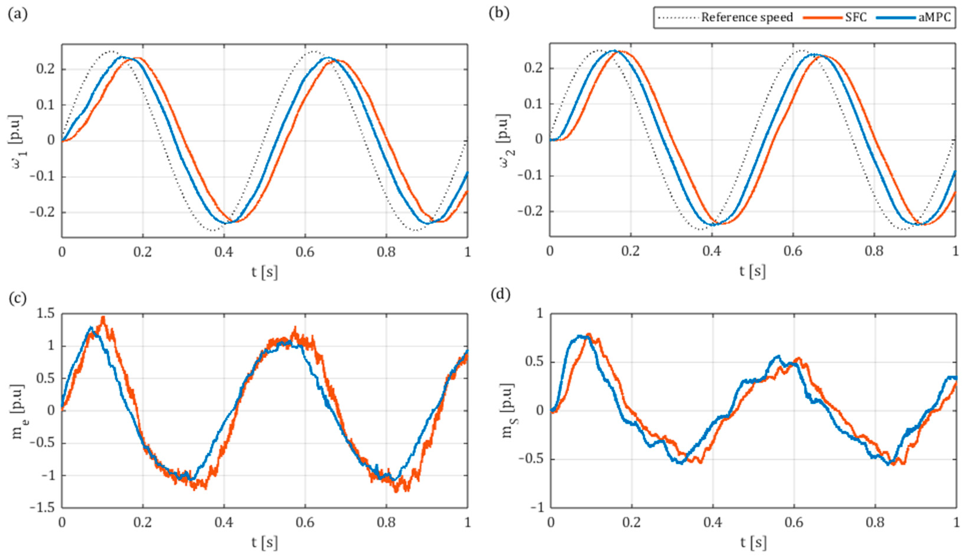
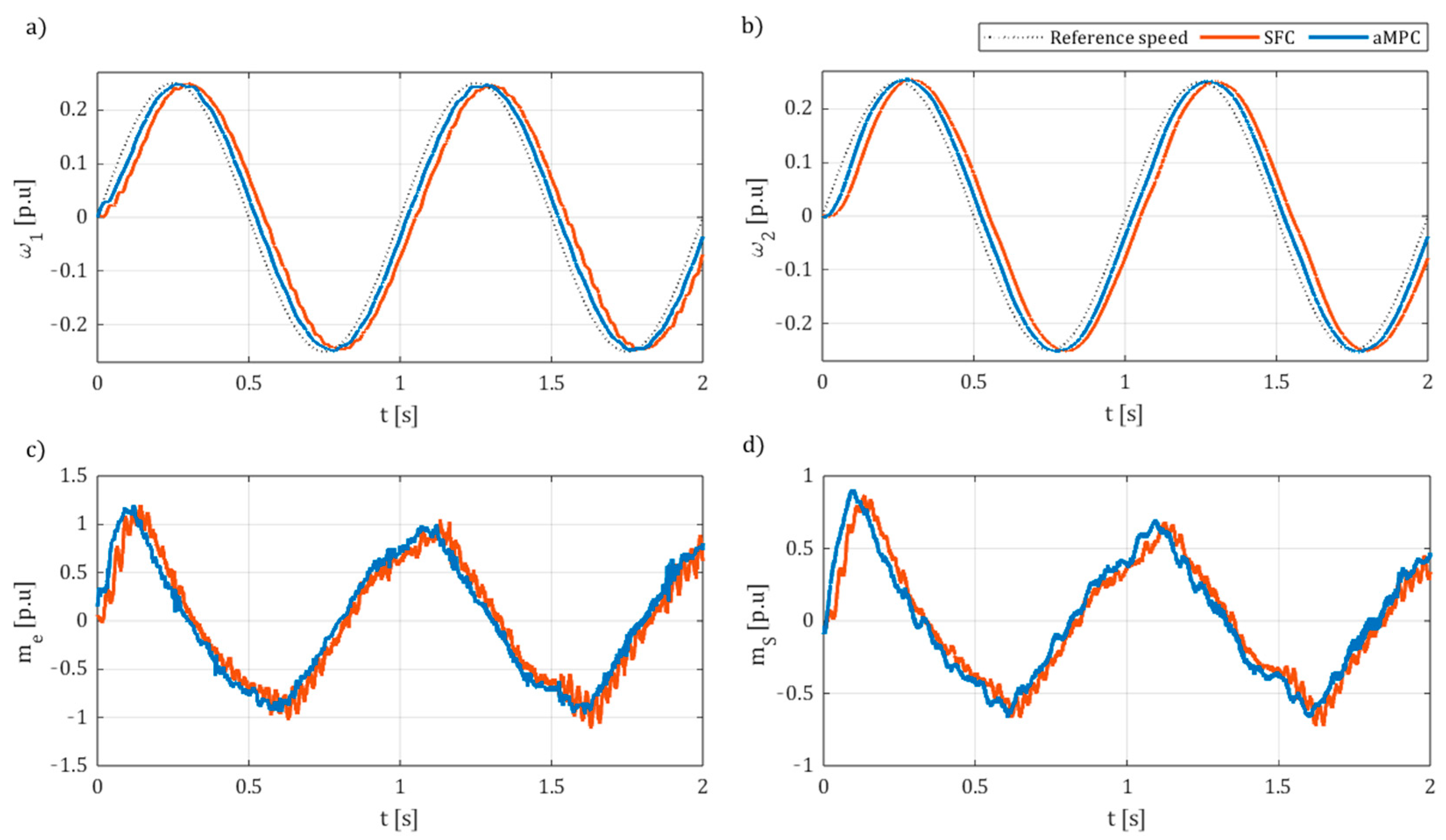
In Figure 20, comparative experimental results for sine wave tracking are showcased. In this case, it is evident from the electromagnetic torque trajectories (Figure 20c) that the initial system response was quicker in the case of aMPC. This resulted in a delay between the reference and the load speed at around $t_d=37 \mathrm{m}\mathrm{s}$, whereas for SFC, it was notably longer, at $t_d=62 \mathrm{m}\mathrm{s}$ (Figure 20b). Moreover, the SFC sinusoidal speed trajectory exhibited an amplitude of 89.9% of the reference and a phase difference of –37.9°, while for aMPC, a slightly higher gain of 93.3% of the reference amplitude and a much shorter phase lag of –21.5° were obtained. Nevertheless, both controllers were capable of achieving near-perfect sinusoidal speed trajectories. Similarly to previous tests, the torque transients for aMPC were distinguished by a lower degree of fluctuations.

In a subsequent set of tests, the control systems were evaluated under modified load conditions. A steel disk with corresponding time constant of $T=0.2 \mathrm{s}$ was mounted on the load side of the shaft, increasing the overall load time constant ratio to $T_2/T_{2N}=1.7$. This modification allowed for an experimental assessment of the controllers’ robustness under increased load inertia.

Figure 21 presents the experimental results of the step response to ${\omega }^{ref}=0.25$ under increased $T_2$. The obtained results confirm the findings from the simulation tests shown in Figure 14—while both control structures ensure the correct operation of the drive for elevated $T_2/T_{2N}$ ratios, the proposed aMPC structure demonstrates superior robustness. This is particularly evident in the load speed transients (Figure 21b) during start-up, where the overshoot reaches 16.8% for SFC, compared to 4% in the case of aMPC. Consequently, the settling time for aMPC is shorter, at $t=0.25 \mathrm{s}$ versus $t=0.33 \mathrm{s}$ for SFC. Finally, aMPC provided a notably faster response to the application of load torque (zoomed section in Figure 21b).

Lastly, comparative results for sine wave tracking under increased $T_2$ are illustrated in Figure 22. Both controllers were able to achieve near-ideal reference amplitudes—100.4% for aMPC and 99.7% for SFC. However, as with the nominal $T_2$ case, the system response was significantly faster with aMPC. The sine wave time delay equalled $t_d=25 \mathrm{m}\mathrm{s}$ for aMPC, whereas in the case of SFC, it was twice as long, at $t_d=51 \mathrm{m}\mathrm{s}$. These delays correspond to phase errors of –9.1° and –18.3° for aMPC and SFC, respectively.

A comparison of these time delays with those noted in Figure 20 further highlights the superior robustness of aMPC. Under nominal parameters, aMPC achieved a phase difference approximately 40% lower than that of SFC. Following the increase in $T_2$, aMPC exhibited a more than 50% smaller phase difference than that observed with SFC.

7. Discussion and Conclusions

In this paper, the issues related to the suppression of torsional vibrations in two-mass electric drives were presented, along with an overview of the main solutions proposed in the literature. As MPC frequently proves impossible to implement in real-time for such systems, a modified linear Analytical MPC system was put forward and compared to a conventional SFC-based control system. The findings of the study, based on the simulation and experimental tests, indicate that the application of the proposed aMPC controller facilitates the correct operation of the two-mass drive and reduces the torsional vibrations of the flexible shaft, while providing higher dynamics and smoother torque control than the conventionally implemented SFC.

• It has been demonstrated that the dynamics of the aMPC controller depend on four parameters simultaneously—namely sampling time $T_s,$ prediction horizon $N$, control horizon $N_u$, and gain coefficient $R$. In this regard, it is recommended that the sampling time is selected first in accordance with the capabilities and physical limitations of the considered system. Furthermore, it was explained that extending the control horizon substantially increases the computational complexity of the controller, and only the first control signal is applied to the object. Therefore, its value should remain at $N_u=1$.
• This leaves two remaining parameters, whose impact on the performance of the controller was presented in the article. Additionally, a performance function, $f$, was proposed, which may be used as the minimised objective function for automated tuning, in this case, with the implementation of GA.
• In the simulation results, a comparison between the aMPC and SFC systems indicated that the proposed aMPC system may display better dynamics and higher robustness to changes of load time constant $T_2$ over a wide range, ensuring better performance for high $T_2/T_{2N}$ ratios and remaining stable for very low $T_2/T_{2N}$ ratios.
• The developed predictive controller was also able to be successfully implemented online in the laboratory setup. Valid results were obtained for similar controller parameters to those of the simulation model automatically optimised by the GA, confirming its applicability in the tuning process. The main advantage of the proposed system in comparison to conventional SFC is the ability to reach similarly high or even better dynamics with much smoother electromagnetic torque transients. Additionally, the superior robustness and better dynamics of aMPC were showcased for higher load inertia. However, the accurate estimation of the state variables, including the load torque, is imperative for the effective operation of aMPC. In this instance, it was observed that the employment of a classical Luenberger observer resulted in oscillations of the state variables during the load torque switching on and off.
• As the performance of the proposed solution relies on the quality of state variable estimation, further studies could include a comparison of the performance of aMPC for different methods of estimation presented in the literature. Additionally, the present study does not undertake a comparison between the performance and robustness of the proposed aMPC and other predictive control approaches, such as the explicit MPC. This aspect could be considered for future work to further contextualise the proposed solution within the broader landscape of predictive control methods.

References

1. Yakub, M.F.M.; Qadir, A.; Aminudin, B.A. Comparative Study on Control Method for Two-Mass Systems. Int. J. Adv. Sci. Eng. Inf. Technol. 2012, 2, 261–266. [Google Scholar] [CrossRef]
2. Shao, N.; Zhou, Q.; Shao, C.; Zhao, Y. Adaptive Control of Robot Series Elastic Drive Joint Based on Optimized Radial Basis Function Neural Network. Int. J. Soc. Robot. 2021, 13, 1823–1832. [Google Scholar] [CrossRef]
3. Jin, X.; Wang, J.; He, X.; Yan, Z.; Xu, L.; Wei, C. Improving Vibration Performance of Electric Vehicles Based on In-Wheel Motor-Active Suspension System via Robust Finite Frequency Control. IEEE Trans. Intell. Transp. Syst. 2023, 24, 1631–1643. [Google Scholar] [CrossRef]
4. Zhang, G. Comparison of control schemes for two-inertia system. In Proceedings of the IEEE 1999 International Conference on Power Electronics and Drive Systems PEDS’99, Hong Kong, China, 27–29 July 1999. [Google Scholar] [CrossRef]
5. Goubej, M. Fundamental performance limitations in PID controlled elastic two-mass systems. In Proceedings of the 2016 IEEE International Conference on Advanced Intelligent Mechatronics (AIM), Banff, Canada, 12–15 July 2016. [Google Scholar] [CrossRef]
6. Szabat, K.; Orłowska-Kowalska, T. Vibration Suppression in a Two-Mass Drive System Using PI Speed Controller and Additional Feedbacks—Comparative Study. IEEE Trans. Ind. Electron. 2007, 54, 1193–1206. [Google Scholar] [CrossRef]
7. Zhang, G.; Furusho, J. Speed control of two-inertia system by PI/PID control. IEEE Trans. Ind. Electron. 2000, 47, 603–609. [Google Scholar] [CrossRef]
8. Li, X.; Shang, D.; Li, H.; Li, F. Resonant Suppression Method Based on PI control for Serial Manipulator Servo Drive System. Sci. Prog. 2020, 103, 36850420950130. [Google Scholar] [CrossRef]
9. Kahsay, A.H.; Derugo, P.; Szabat, K.; Katsura, S. Design of Disturbance Observer-Based Robust Speed Control Structure for Two-Mass Drive System with the Help of Birch Optimization Algorithm. Energies 2025, 18, 1914. [Google Scholar] [CrossRef]
10. Wróbel, K.; Śleszycki, K. Robust states controller for two mass system. Przegląd Elektrotechniczny 2023, 99, 9–12. [Google Scholar] [CrossRef]
11. Szczepański, R.; Kamiński, M.; Tarczewski, T. Auto-Tuning Process of State Feedback Speed Controller Applied for Two-Mass System. Energies 2020, 13, 3067. [Google Scholar] [CrossRef]
12. Wang, C.; Wang, T.; Chen, G.; Pan, J. Automatic Detection and Self-Adjustment Compensation for Mechanical Oscillations and Disturbances in Servo Systems. IEEE Trans. Syst. Man Cybern. Syst. 2024, 54, 1180–1190. [Google Scholar] [CrossRef]
13. Serkies, P.; Szabat, K. Effective damping of the torsional vibrations of the drive system with an elastic joint based on the forced dynamic control algorithms. J. Vib. Control. 2019, 25, 2225–2236. [Google Scholar] [CrossRef]
14. Sariyildiz, E.; Yu, H.; Nozaki, T.; Murakami, T. Robust vibration control of two-mass resonant systems in state space. In Proceedings of the 2016 IEEE 14th International Workshop on Advanced Motion Control (AMC), Auckland, New Zealand, 22–24 April 2016. [Google Scholar] [CrossRef]
15. Vittek, J.; Ryvkin, S. Decomposed Sliding Mode Control of the Drive with Interior Permanent Magnet Synchronous Motor and Flexible Coupling. Math. Probl. Eng. 2013, 2013, 680376. [Google Scholar] [CrossRef]
16. Wang, C.; Liu, F.; Xu, J.; Pan, J. A SMC-Based Accurate and Robust Load Speed Control Method for Elastic Servo System. IEEE Trans. Ind. Electron. 2024, 71, 2300–2308. [Google Scholar] [CrossRef]
17. Lukichev, D.V.; Demidova, G.L. PID-type fuzzy adaptive control for two-mass servo-drive system: Design, simulation and experiment. In Proceedings of the 2016 IX International Conference on Power Drives Systems (ICPDS), Perm, Russia, 3–7 October 2016. [Google Scholar] [CrossRef]
18. Vukojičić, S.; Ristić, L.; Kvaščev, G. Comparation between PI and Model Predictive Control of Two Mass Resonant Mechanical System. In Proceedings of the 7th International Conference on Environment Friendly Energies and Applications (EFEA), Bagatelle Moka MU, Mauritius, 13–16 December 2022. [Google Scholar] [CrossRef]
19. Kaczmarczyk, G.; Stanislawski, R.; Kamiński, M. Deep-Learning Techniques Applied for State-Variables Estimation of Two-Mass System. Energies 2025, 18, 568. [Google Scholar] [CrossRef]
20. Thomsen, S.; Hoffmann, N.; Fuchs, F.W. Comparative study of conventional PI-control, PI-based state space control and model based predictive control for drive systems with elastic coupling. In Proceedings of the 2010 IEEE Energy Conversion Congress and Exposition, Atlanta, GA, USA, 12–16 September 2010. [Google Scholar] [CrossRef]
21. Serkies, P.; Szabat, K. Application of the MPC to the Position Control of the Two-Mass Drive System. IEEE Trans. Ind. Electron. 2013, 60, 3679–3688. [Google Scholar] [CrossRef]
22. Wang, C.; Yang, M.; Zheng, W.; Long, J.; Xu, D. Vibration Suppression with Shaft Torque Limitation Using Explicit MPC-PI Switching Control in Elastic Drive Systems. IEEE Trans. Ind. Electron. 2015, 62, 6855–6867. [Google Scholar] [CrossRef]
23. Fuentes, E.J.; Silva, C.A.; Yuz, J.I. Predictive Speed Control of a Two-Mass System Driven by a Permanent Magnet Synchronous Motor. IEEE Trans. Ind. Electron. 2012, 59, 2840–2848. [Google Scholar] [CrossRef]
24. Kouro, S.; Perez, M.A.; Rodriguez, J.; Llor, A.M.; Young, H.A. Model Predictive Control: MPC’s Role in the Evolution of Power Electronics. IEEE Ind. Electron. Mag. 2015, 9, 8–21. [Google Scholar] [CrossRef]
25. Nguyen, T.T.; Nguyen, T.H.; Jeon, J.W. Explicit Model Predictive Speed Control for Permanent Magnet Synchronous Motor with Torque Ripple Minimization. IEEE Access 2023, 11, 134199–134210. [Google Scholar] [CrossRef]
26. Wróbel, K.; Szabat, K.; Serkies, P. Long-horizon model predictive control of induction motor drive. Arch. Electr. Eng. 2019, 68, 569–593. [Google Scholar] [CrossRef]
27. Karg, B.; Lucia, S. Efficient Representation and Approximation of Model Predictive Control Laws via Deep Learning. IEEE Trans. Cybern. 2020, 50, 3866–3878. [Google Scholar] [CrossRef] [PubMed]
28. Abu-Ali, M.; Berkel, F.; Manderla, M.; Reimann, S.; Kennel, R.; Abdelrahem, M. Deep Learning-Based Long-Horizon MPC: Robust, High Performing, and Computationally Efficient Control for PMSM Drives. IEEE Trans. Power Electron. 2022, 37, 12486–12501. [Google Scholar] [CrossRef]
29. Chaber, P.; Ławryńczuk, M. Fast Analytical Model Predictive Controllers and Their Implementation for STM32 ARM Microcontroller. IEEE Trans. Ind. Inform. 2019, 15, 4580–4590. [Google Scholar] [CrossRef]
Figure 1. Two-mass motor drive model.
Actuators 14 00254 g001
Figure 2. Block diagram of the two-mass system.
Actuators 14 00254 g002
Figure 3. Block diagram of the proposed SFC.
Actuators 14 00254 g003
Figure 4. Block diagram of the proposed aMPC.
Actuators 14 00254 g004
Figure 5. Block diagram of the proposed control structure.
Actuators 14 00254 g005
Figure 6. Performance function f depending on the aMPC parameters: (a) prediction horizon N ; (b) gain coefficient R .
Actuators 14 00254 g006
Figure 7. aMPC performance function value in successive generations of GA optimisation for different population sizes.
Actuators 14 00254 g007
Figure 8. Simulation step response for different lengths of prediction horizon N : (a) motor speed ω 1 ; (b) load speed ω 2 ; (c) electromagnetic torque m e ; (d) shaft torque m s .
Actuators 14 00254 g008
Figure 9. Simulation step response for different values of gain coefficient R : (a) motor speed ω 1 ; (b) load speed ω 2 ; (c) electromagnetic torque m e ; (d) shaft torque m s .
Actuators 14 00254 g009
Figure 10. Simulation step response for different values of prediction horizon N u : (a) motor speed ω 1 ; (b) load speed ω 2 ; (c) electromagnetic torque m e ; (d) shaft torque m s .
Actuators 14 00254 g010
Figure 11. Comparative simulation results of step response of aMPC and SFC for reference speed ω r e f = 0.25   p . u . : (a) motor speed ω 1 ; (b) load speed ω 2 ; (c) electromagnetic torque m e ; (d) shaft torque m s .
Actuators 14 00254 g011
Figure 12. Comparative simulation results of step response of aMPC and SFC for reference speed ω r e f = 0.1   p . u . : (a) motor speed ω 1 ; (b) load speed ω 2 ; (c) electromagnetic torque m e ; (d) shaft torque m s .
Actuators 14 00254 g012
Figure 13. The comparison of performance function f depending on the load time constant T 2 .
Actuators 14 00254 g013
Figure 14. Comparative simulation results of step response of aMPC and SFC for different values of load time constant T 2 : (a) motor speed ω 1 ; (b) load speed ω 2 ; (c) electromagnetic torque m e ; (d) shaft torque m s .
Actuators 14 00254 g014
Figure 15. Two-mass DC motor drive laboratory setup.
Actuators 14 00254 g015
Figure 16. Schematic diagram of the laboratory setup.
Actuators 14 00254 g016
Figure 17. Block diagram of the experimental control structure in MATLAB/Simulink.
Actuators 14 00254 g017
Figure 18. Comparative experimental results of step response of aMPC and SFC for reference speed ω r e f = 0.25   p . u . : (a) motor speed ω 1 ; (b) load speed ω 2 ; (c) electromagnetic torque m e ; (d) shaft torque m s .
Actuators 14 00254 g018
Figure 19. Comparative experimental results of step response of aMPC and SFC for reference speed ω r e f = 0.5   p . u . : (a) motor speed ω 1 ; (b) load speed ω 2 ; (c) electromagnetic torque m e ; (d) shaft torque m s .
Actuators 14 00254 g019
Figure 20. Comparative experimental results of sine wave tracking of aMPC and SFC for amplitude ω r e f = 0.25   p . u . and frequency f = 2   H z : (a) motor speed ω 1 ; (b) load speed ω 2 ; (c) electromagnetic torque m e ; (d) shaft torque m s .
Actuators 14 00254 g020
Figure 21. Comparative experimental results of step response of aMPC and SFC for reference speed ω r e f = 0.25   p . u . and higher load time constant ratio T 2 / T 2 N = 1.7 : (a) motor speed ω 1 ; (b) load speed ω 2 ; (c) electromagnetic torque m e ; (d) shaft torque m s .
Actuators 14 00254 g021
Figure 22. Comparative experimental results of sine wave tracking of aMPC and SFC for amplitude ω r e f = 0.25   p . u . , frequency f = 1   H z , and higher load time constant ratio T 2 / T 2 N = 1.7 : (a) motor speed ω 1 ; (b) load speed ω 2 ; (c) electromagnetic torque m e ; (d) shaft torque m s .
Actuators 14 00254 g022