
A Long-Tail Fault Diagnosis Method Based on a Coupled Time–Frequency Attention Transformer

Abstract
1. Introduction
- Addressing the issue of decreased model accuracy caused by long-tail data distribution in real production environments, an innovative CTFAM is proposed, which processes signals in the frequency domain using the FFT while retaining the imaginary part; we also design a real–imaginary attention mechanism to effectively extract important information in the frequency domain.
- Based on CTFAM, an enhanced transformer model called the coupled time–frequency attention transformer (CTFAT) is suggested for precise fault identification and diagnosis. The one-dimensional convolution is applied to the signal to decompose it into blocks, which effectively reduces the influence of high-frequency noise and addresses the issue of excessively long input size due to the length of the signal.
- The model’s diagnostic performance is analyzed using bearing datasets from CWRU and the laboratory. The experimental results demonstrate that, compared to other related methods, the model exhibits exceptional generalization ability and anti-interference capabilities in complex environments, especially when dealing with long-tailed data samples.
2. Related Work
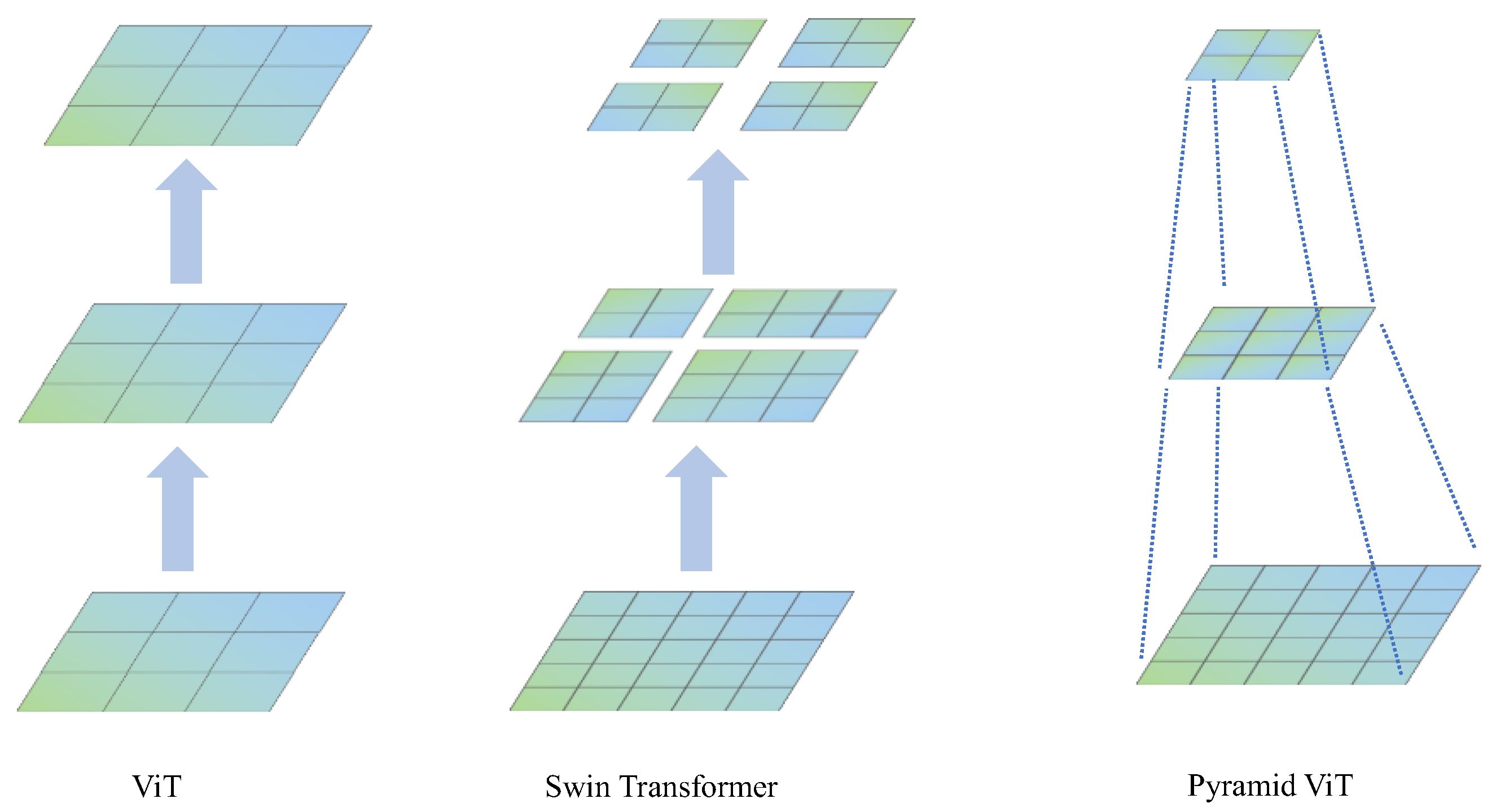
2.1. Transformer Attention Network
2.2. Improved Transformer Model
3. Method
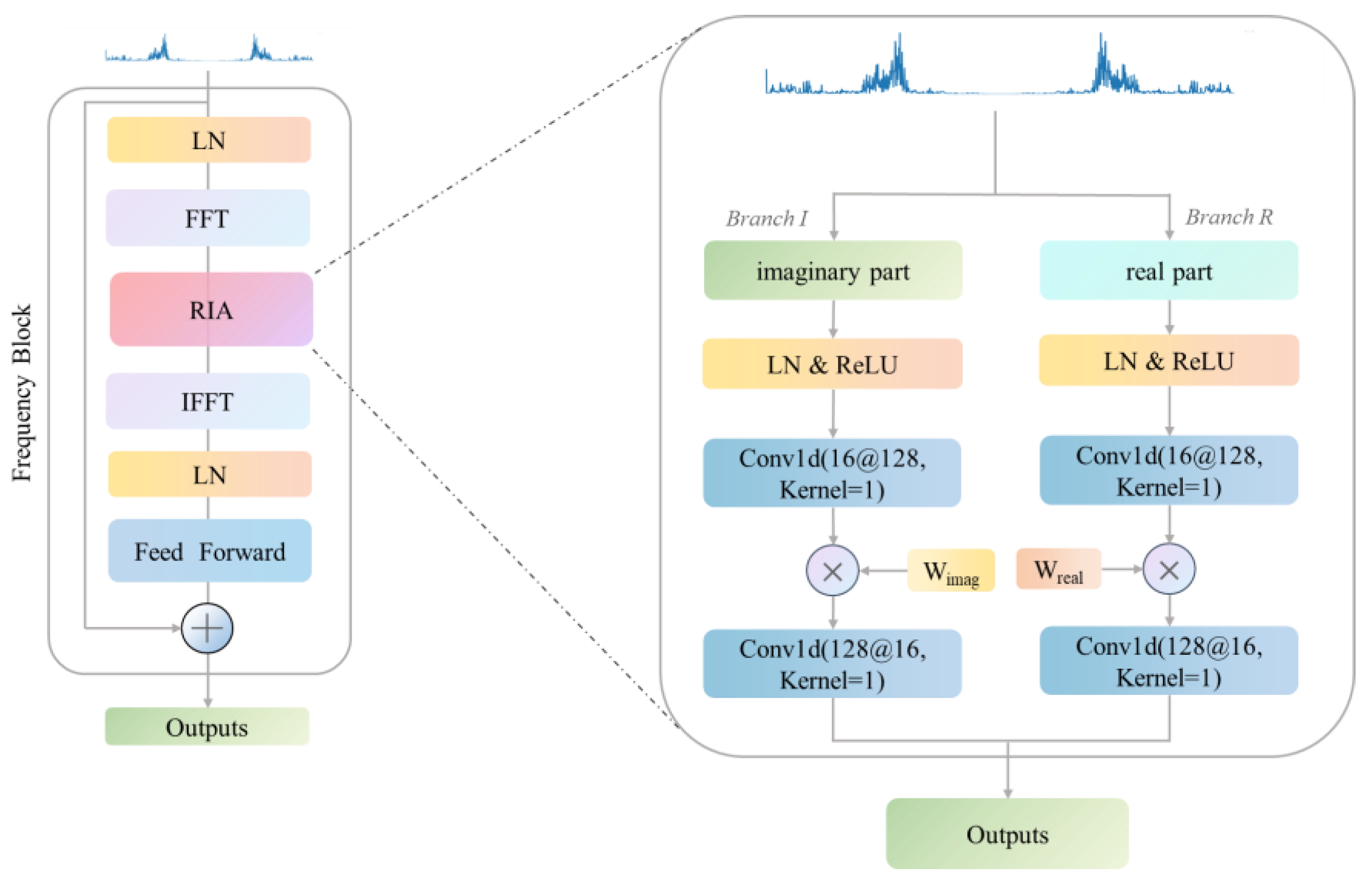
3.1. Real–Imaginary Attention
3.2. Coupled Time–Frequency Attention Mechanism
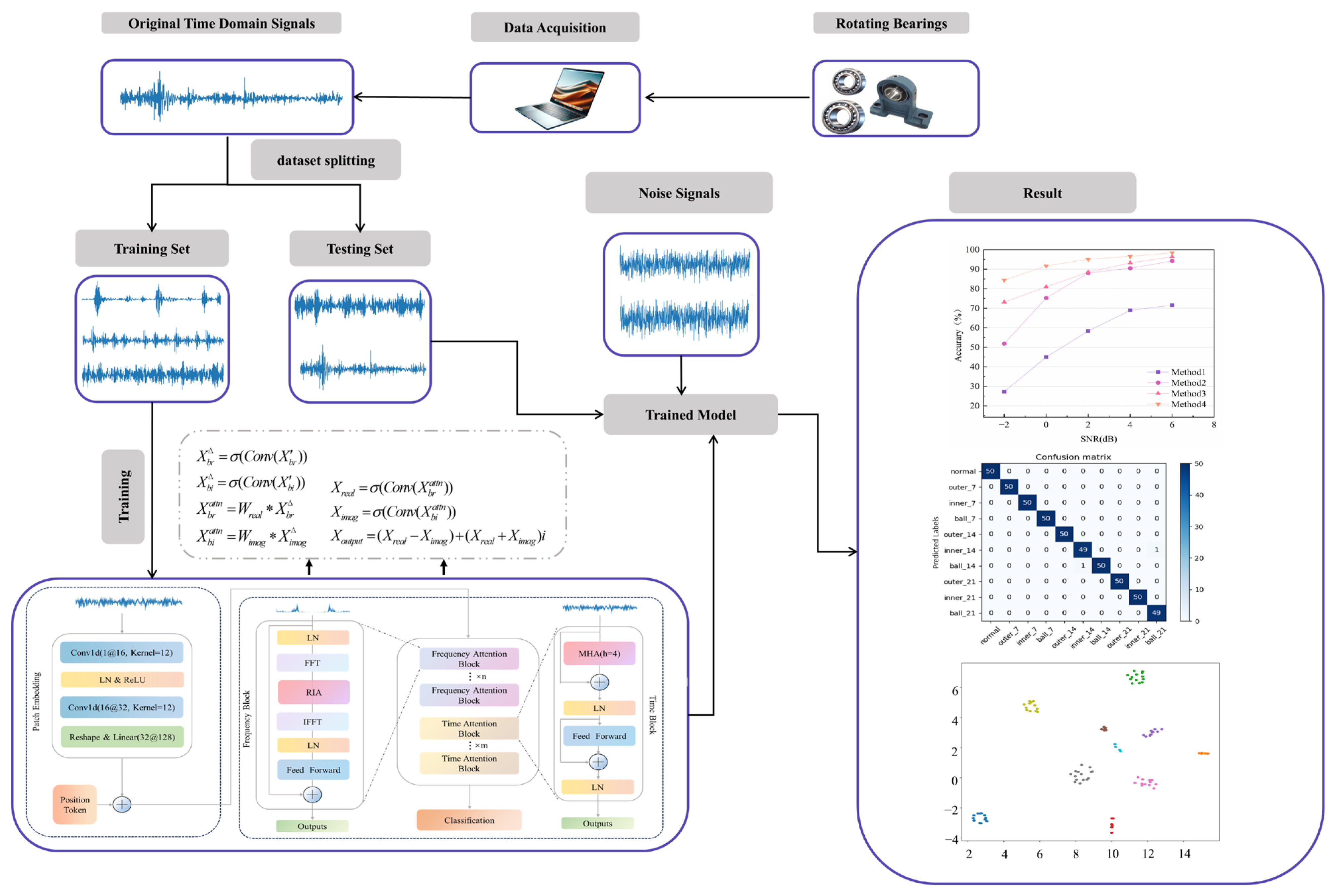
3.3. Coupled Time–Frequency Attention Transformer Model
4. Experiment
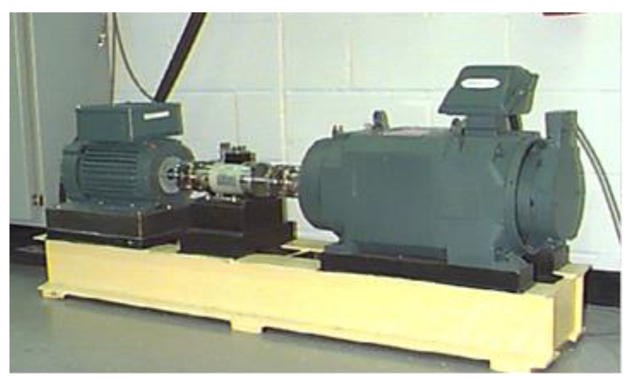
4.1. Experimental Environment and Dataset Introduction
4.2. Data Processing
- (1)
- According to the sample frequency, the window length is set at 1024 data points in order to strike a reasonable balance between frequency precision and time resolution. This configuration maintains enough temporal locality to record the time-domain features of fault impacts while also guaranteeing the capacity to discern the distinctive frequencies of bearing faults.
- (2)
- To effectively mitigate the spectral leakage caused by the non-integer periodic truncation of bearing fault impact signals, a Hanning window is applied to the signals. The reliability of characteristic frequency band identification is significantly increased by this procedure, which means that the amplitude peaks at the fault frequencies more properly reflect the energy distribution. The specific operational procedure is as follows. First, position the Hanning window at the starting point of the signal sequence. Subsequently, slide the window along the time axis at a fixed stride to achieve segmented processing of the signal.
- (3)
- At each location, extract the subsequences within the window as a sample.
4.3. Case 1: CWRU Public Bearing Dataset
4.4. Case 2: Laboratory Bearing Dataset
5. Conclusions
Author Contributions
Funding
Informed Consent Statement
Data Availability Statement
Conflicts of Interest
Abbreviations
| Acronym | Meaning |
| FFT | Fast Fourier Transform |
| CWRU | Case Western Reserve University |
| CNN | Convolutional Neural Networks |
| PCA | Principal Component Analysis |
| SVM | Support Vector Machine |
| PSO | Particle Swarm Optimization |
| RF | Random Forest |
| RNN | Recurrent Neural Networks |
| GAN | Generative Adversarial Networks |
| VMD | Variational Mode Decomposition |
| SDP | Symmetric Dot Pattern |
| CA | Coordinate Attention |
| GRU | Gated Recurrent Unit |
| BiGRU | Bidirectional Gated Recurrent Units |
| SSDL | Self-training Semi-supervised Deep Learning |
| MCSwin-T | Multi-channel Calibrated Transformer with Shifted Windows |
| CTFAM | Coupled Time–Frequency Attention Mechanism |
| CTFAT | Coupled Time–Frequency Attention Transformer |
| ViT | Vision Transformer |
| RIA | Real-Imaginary Attention |
| LN | Layer Normalization |
| IFFT | Inverse Fast Fourier Transform |
| IR | Inner Race |
| OR | Outer Race |
| RE | Rolling Elements |
References
- Chen, Z.X.; Yang, Y.; He, C.B.; Liu, Y.B.; Liu, X.Z.; Cao, Z. Feature Extraction Based on Hierarchical Improved Envelope Spectrum Entropy for Rolling Bearing Fault Diagnosis. IEEE Trans. Instrum. Meas. 2023, 72, 1–12. [Google Scholar] [CrossRef]
- Liu, G.Z.; Wu, L.F. Incremental bearing fault diagnosis method under imbalanced sample conditions. Comput. Ind. Eng. 2024, 192, 110203. [Google Scholar] [CrossRef]
- Wang, G.; Liu, D.D.; Cui, L.L. Auto-Embedding Transformer for Interpretable Few-Shot Fault Diagnosis of Rolling Bearings. IEEE Trans. Reliab. 2024, 73, 1270–1279. [Google Scholar] [CrossRef]
- Wu, X.G.; Peng, H.D.; Cui, X.Y.; Guo, T.W.; Zhang, Y.T. Multichannel Vibration Signal Fusion Based on Rolling Bearings and MRST-Transformer Fault Diagnosis Model. IEEE Sens. J. 2024, 24, 16336–16346. [Google Scholar] [CrossRef]
- Zhao, K.C.; Xiao, J.Q.; Li, C.; Xu, Z.F.; Yue, M.N. Fault diagnosis of rolling bearing using CNN and PCA fractal based feature extraction. Measurement 2023, 223, 113754. [Google Scholar] [CrossRef]
- Wu, Y.Q.; Dai, J.Y.; Yang, X.Q.; Shao, F.M.; Gong, J.C.; Zhang, P.; Liu, S.D. The Fault Diagnosis of Rolling Bearings Based on FFT-SE-TCN-SVM. Actuators 2025, 14, 152. [Google Scholar] [CrossRef]
- Aburakhia, S.A.; Myers, R.; Shami, A. A Hybrid Method for Condition Monitoring and Fault Diagnosis of Rolling Bearings With Low System Delay. IEEE Trans. Instrum. Meas. 2022, 71, 1–13. [Google Scholar] [CrossRef]
- Hakim, M.; Omran, A.A.B.; Ahmed, A.N.; Al-Waily, M.; Abdellatif, A. A systematic review of rolling bearing fault diagnoses based on deep learning and transfer learning: Taxonomy, overview, application, open challenges, weaknesses and recommendations. Ain Shams Eng. J. 2023, 14, 101945. [Google Scholar] [CrossRef]
- Chen, X.H.; Zhang, B.K.; Gao, D. Bearing fault diagnosis base on multi-scale CNN and LSTM model. J. Intell. Manuf. 2021, 32, 971–987. [Google Scholar] [CrossRef]
- Zhao, X.; Chen, S.; Gao, K.; Luo, L. Bidirectional Recurrent Neural Network based on Multi-Kernel Learning Support Vector Machine for Transformer Fault Diagnosis. Int. J. Adv. Comput. Sci. Appl. 2023, 14, 125–135. [Google Scholar] [CrossRef]
- Shao, H.; Li, W.; Cai, B.; Wan, J.; Xiao, Y.; Yan, S. Dual-Threshold Attention-Guided GAN and Limited Infrared Thermal Images for Rotating Machinery Fault Diagnosis Under Speed Fluctuation. IEEE Trans. Ind. Inform. 2023, 19, 9933–9942. [Google Scholar] [CrossRef]
- Zhi, S.D.; Su, K.Y.; Yu, J.; Li, X.Y.; Shen, H.K. An unsupervised transfer learning bearing fault diagnosis method based on multi-channel calibrated Transformer with shiftable window. Struct. Health Monit. Int. J. 2025, 34, 14759217251324671. [Google Scholar] [CrossRef]
- Zhang, J.B.; Zhao, Z.Q.; Jiao, Y.H.; Zhao, R.C.; Hu, X.L.; Che, R.W. DPCCNN: A new lightweight fault diagnosis model for small samples and high noise problem. Neurocomputing 2025, 626, 129526. [Google Scholar] [CrossRef]
- Wang, Z.Y.; Xu, X.; Song, D.L.; Zheng, Z.J.; Li, W.D. A Novel Bearing Fault Diagnosis Method Based on Improved Convolutional Neural Network and Multi-Sensor Fusion. Machines 2025, 13, 216. [Google Scholar] [CrossRef]
- Mansouri, M.; Dhibi, K.; Hajji, M.; Bouzara, K.; Nounou, H.; Nounou, M. Interval-Valued Reduced RNN for Fault Detection and Diagnosis for Wind Energy Conversion Systems. IEEE Sens. J. 2022, 22, 13581–13588. [Google Scholar] [CrossRef]
- Niu, J.; Pan, J.; Qin, Z.; Huang, F.; Qin, H. Small-Sample Bearings Fault Diagnosis Based on ResNet18 with Pre-Trained and Fine-Tuned Method. Appl. Sci. 2024, 14, 5360. [Google Scholar] [CrossRef]
- Zhou, F.N.; Yang, S.; Fujita, H.; Chen, D.M.; Wen, C.L. Deep learning fault diagnosis method based on global optimization GAN for unbalanced data. Knowl. Based Syst. 2020, 187, 104837. [Google Scholar] [CrossRef]
- Chen, Y.S.; Qiang, Y.K.; Chen, J.H.; Yang, J.L. FMRGAN: Feature Mapping Reconstruction GAN for Rolling Bearings Fault Diagnosis Under Limited Data Condition. IEEE Sens. J. 2024, 24, 25116–25131. [Google Scholar] [CrossRef]
- Peng, P.; Lu, J.X.; Tao, S.T.; Ma, K.; Zhang, Y.; Wang, H.W.; Zhang, H.M. Progressively Balanced Supervised Contrastive Representation Learning for Long-Tailed Fault Diagnosis. IEEE Trans. Instrum. Meas. 2022, 71, 1–12. [Google Scholar] [CrossRef]
- Huang, M.; Sheng, C.X. Adaptive-conditional loss and correction module enhanced informer network for long-tailed fault diagnosis of motor. J. Comput. Des. Eng. 2024, 11, 306–318. [Google Scholar] [CrossRef]
- Luo, H.; Wang, X.Y.; Zhang, L. Normalization-Guided and Gradient-Weighted Unsupervised Domain Adaptation Network for Transfer Diagnosis of Rolling Bearing Faults Under Class Imbalance. Actuators 2025, 14, 39. [Google Scholar] [CrossRef]
- Jian, C.X.; Mo, G.P.; Peng, Y.H.; Ao, Y.H. Long-tailed multi-domain generalization for fault diagnosis of rotating machinery under variable operating conditions. Struct. Health Monit. Int. J. 2024, 24, 1927–1945. [Google Scholar] [CrossRef]
- Zhang, X.; He, C.; Lu, Y.P.; Chen, B.A.; Zhu, L.; Zhang, L. Fault diagnosis for small samples based on attention mechanism. Measurement 2022, 187, 110242. [Google Scholar] [CrossRef]
- Liu, Y.; Wen, W.G.; Bai, Y.H.; Meng, Q.Z. Self-supervised feature extraction via time-frequency contrast for intelligent fault diagnosis of rotating machinery. Measurement 2023, 210, 112551. [Google Scholar] [CrossRef]
- Long, J.Y.; Chen, Y.B.; Yang, Z.; Huang, Y.W.; Li, C. A novel self-training semi-supervised deep learning approach for machinery fault diagnosis. Int. J. Prod. Res. 2023, 61, 8238–8251. [Google Scholar] [CrossRef]
- Chen, Z.H.; Chen, J.L.; Liu, S.; Feng, Y.; He, S.L.; Xu, E.Y. Multi-channel Calibrated Transformer with Shifted Windows for few-shot fault diagnosis under sharp speed variation. Isa Trans. 2022, 131, 501–515. [Google Scholar] [CrossRef]
- Wang, H.; Liu, Z.L.; Peng, D.D.; Cheng, Z. Attention-guided joint learning CNN with noise robustness for bearing fault diagnosis and vibration signal denoising. Isa Trans. 2022, 128, 470–484. [Google Scholar] [CrossRef]
- Chen, B.A.; Liu, T.T.; He, C.; Liu, Z.C.; Zhang, L. Fault Diagnosis for Limited Annotation Signals and Strong Noise Based on Interpretable Attention Mechanism. IEEE Sens. J. 2022, 22, 11865–11880. [Google Scholar] [CrossRef]
- Ding, Y.F.; Jia, M.P.; Miao, Q.H.; Cao, Y.D. A novel time-frequency Transformer based on self-attention mechanism and its application in fault diagnosis of rolling bearings. Mech. Syst. Signal Process. 2022, 168, 108616. [Google Scholar] [CrossRef]
- Qin, Z.Q.; Zhang, P.Y.; Wu, F.; Li, X. FcaNet: Frequency Channel Attention Networks. In Proceedings of the 18th IEEE/CVF International Conference on Computer Vision (ICCV), Electr Network, Montreal, QC, Canada, 11–17 October 2021; pp. 763–772. [Google Scholar]
- Zhao, H.S.; Jia, J.; Koltun, V. Exploring Self-attention for Image Recognition. In Proceedings of the IEEE/CVF Conference on Computer Vision and Pattern Recognition (CVPR), Electr Network, Seattle, DC, USA, 14–19 June 2020; pp. 10073–10082. [Google Scholar]
- Han, K.; Wang, Y.; Chen, H.; Chen, X.; Guo, J.; Liu, Z.; Tang, Y.; Xiao, A.; Xu, C.; Xu, Y.; et al. A Survey on Vision Transformer. IEEE Trans. Pattern Anal. Mach. Intell. 2023, 45, 87–110. [Google Scholar] [CrossRef]
- Liu, Z.; Lin, Y.; Cao, Y.; Hu, H.; Wei, Y.; Zhang, Z.; Lin, S.; Guo, B. Swin Transformer: Hierarchical Vision Transformer using Shifted Windows. In Proceedings of the 2021 IEEE/CVF International Conference on Computer Vision (ICCV), Montreal, QC, Canada, 10–17 October 2021; pp. 9992–10002. [Google Scholar]
- Wang, W.; Xie, E.; Li, X.; Fan, D.P.; Song, K.; Liang, D.; Lu, T.; Luo, P.; Shao, L. Pyramid Vision Transformer: A Versatile Backbone for Dense Prediction without Convolutions. In Proceedings of the 2021 IEEE/CVF International Conference on Computer Vision (ICCV), Montreal, QC, Canada, 10–17 October 2021; pp. 548–558. [Google Scholar]
- Bai, X.; Ma, Z.; Meng, G. Bearing Fault Diagnosis Based on Wavelet Transform and Residual Shrinkage Network. In Proceedings of the 2022 International Conference on Computer Network, Electronic and Automation (ICCNEA), Xi’an, China, 23–25 September 2022; pp. 373–378. [Google Scholar]
- Liu, Y. One-level Stationary Wavelet Packet Transform & Hilbert Transform based Rolling Bearing Fault Diagnosis. In Proceedings of the 2018 IEEE International Conference on Information and Automation (ICIA), Wuyishan, China, 11–13 August 2018; pp. 1475–1479. [Google Scholar]
- Yang, C.P.; Qiao, Z.J.; Zhu, R.H.; Xu, X.F.; Lai, Z.H.; Zhou, S.T. An Intelligent Fault Diagnosis Method Enhanced by Noise Injection for Machinery. IEEE Trans. Instrum. Meas. 2023, 72, 1–11. [Google Scholar] [CrossRef]
- Smith, W.A.; Randall, R.B. Rolling element bearing diagnostics using the Case Western Reserve University data: A benchmark study. Mech. Syst. Signal Process. 2015, 64–65, 100–131. [Google Scholar] [CrossRef]
- Zhang, L.; Gu, S.; Luo, H.; Ding, L.; Guo, Y. Residual Shrinkage ViT with Discriminative Rebalancing Strategy for Small and Imbalanced Fault Diagnosis. Sensors 2024, 24, 890. [Google Scholar] [CrossRef]


| Structural Name | IR/mm | OR/mm | Rolling Element Diameter/mm | Pitch Diameter/mm | Limiting Speed r/min | Ball No. | Weight /kg |
|---|---|---|---|---|---|---|---|
| Parameters | 25 | 52 | 7.94 | 39.04 | 14,000 | 9 | 0.132 |
| Type of Fault | Degree of Damage/mm | Label | Number of Training Samples | Datasets |
|---|---|---|---|---|
| Normal | 0 | 0 | 100 | |
| Inner race fault | 0.118 | 1 | 10/20/30/40/50 | A/B/C/D/E |
| 0.356 | 2 | |||
| 0.533 | 3 | |||
| Outer race fault | 0.118 | 4 | ||
| 0.356 | 5 | |||
| 0.533 | 6 | |||
| Ball fault | 0.118 | 7 | ||
| 0.356 | 8 | |||
| 0.533 | 9 |
| Type of Fault | Motor Speed | Fault Position |
|---|---|---|
| Normal | 1000 r/min |  |
| Inner race fault | 1000 r/min |  |
| Outer race fault | 1000 r/min | 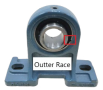 |
| Ball fault | 1000 r/min | 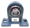 |
| Type of Fault | Degree of Damage/mm | Label | Number of Training Samples | Datasets |
|---|---|---|---|---|
| Normal | None | 0 | 100 | |
| Inner race fault | Slight | 1 | 10/20/30/40/50 | A/B/C/D/E |
| moderate | 2 | |||
| severe | 3 | |||
| Outer race fault | Slight | 4 | ||
| moderate | 5 | |||
| severe | 6 | |||
| Ball fault | Slight | 7 | ||
| moderate | 8 | |||
| severe | 9 |
| Model | Method 1 | Method 2 | Method 3 | Method 4 |
|---|---|---|---|---|
| Parameters | 6.28M | 10.42M | 26.25M | 2.34M |
| Model Name | Included Module | Accuracy | Precision | Recall | Specificity |
|---|---|---|---|---|---|
| TAT | MHA | 62.81 | 0.6330 | 0.6280 | 0.9587 |
| FAT | RIA | 95.40 | 0.9568 | 0.9540 | 0.9950 |
| CTFAT | RIA + MHA | 99.06 | 0.9909 | 1.000 | 0.9989 |
Disclaimer/Publisher’s Note: The statements, opinions and data contained in all publications are solely those of the individual author(s) and contributor(s) and not of MDPI and/or the editor(s). MDPI and/or the editor(s) disclaim responsibility for any injury to people or property resulting from any ideas, methods, instructions or products referred to in the content. |
© 2025 by the authors. Licensee MDPI, Basel, Switzerland. This article is an open access article distributed under the terms and conditions of the Creative Commons Attribution (CC BY) license (https://creativecommons.org/licenses/by/4.0/).
Share and Cite
Zhang, L.; Zhang, Y.; Luo, H.; Ren, T.; Li, H. A Long-Tail Fault Diagnosis Method Based on a Coupled Time–Frequency Attention Transformer. Actuators 2025, 14, 255. https://doi.org/10.3390/act14050255
Zhang L, Zhang Y, Luo H, Ren T, Li H. A Long-Tail Fault Diagnosis Method Based on a Coupled Time–Frequency Attention Transformer. Actuators. 2025; 14(5):255. https://doi.org/10.3390/act14050255
Chicago/Turabian StyleZhang, Li, Ying Zhang, Hao Luo, Tongli Ren, and Hongsheng Li. 2025. "A Long-Tail Fault Diagnosis Method Based on a Coupled Time–Frequency Attention Transformer" Actuators 14, no. 5: 255. https://doi.org/10.3390/act14050255
APA StyleZhang, L., Zhang, Y., Luo, H., Ren, T., & Li, H. (2025). A Long-Tail Fault Diagnosis Method Based on a Coupled Time–Frequency Attention Transformer. Actuators, 14(5), 255. https://doi.org/10.3390/act14050255