

An Improved Design of a Continuously Variable Transmission Based on Circumferentially Arranged Disks for Enhanced Efficiency in the Low Torque Region

 , ,
, ,
Abstract
1. Introduction
- Analysis of a CAD CVT in the low torque region.
- Proposal of a new mechanical design that overcomes the problem of low efficiency faced by a CAD CVT in low torque regions while maintaining its fundamental theme.
- Development of a stable control system for the force applied to the traction disks of a CAD CVT according to the instantaneous torque requirement.
- New/improved mechanical design of a CAD CVT with better efficiency in low torque regions.
- Design of a stable hydraulic-actuation-based control system for the improved mechanical design of a CAD CVT.
2. Materials and Methods
2.1. Problem Statement
2.2. Analysis of CAD CVT
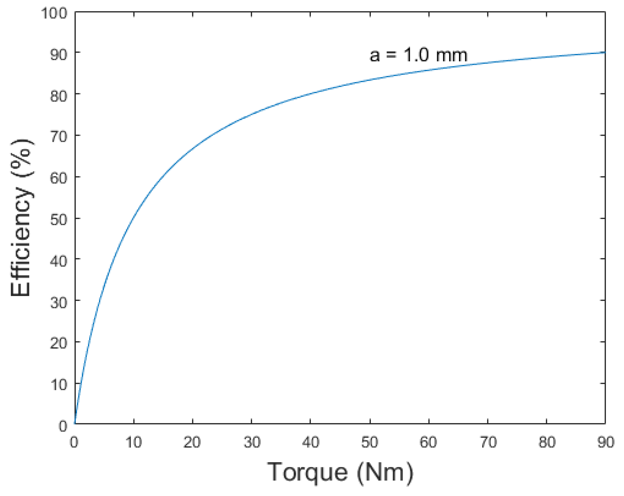
2.2.1. Analysis of CAD CVT Efficiency During Variable-Torque Operation
2.2.2. Root Cause of Efficiency Drop
2.3. Mechanical Design of the Proposed CAD CVT-II
2.3.1. Critical Design Parameters
- Fn, the force applied to the traction disks, can be controlled during operation.
- The new design should apply equal force to all traction disks simultaneously.
- The new design should be such that it can measure the applied torque during operation and adjust the Fn accordingly during operation.
- The new design should be added as an additional feature to the existing CAD CVT so that the mathematical equations derived for the CAD CVT [39] are also valid for the new design.
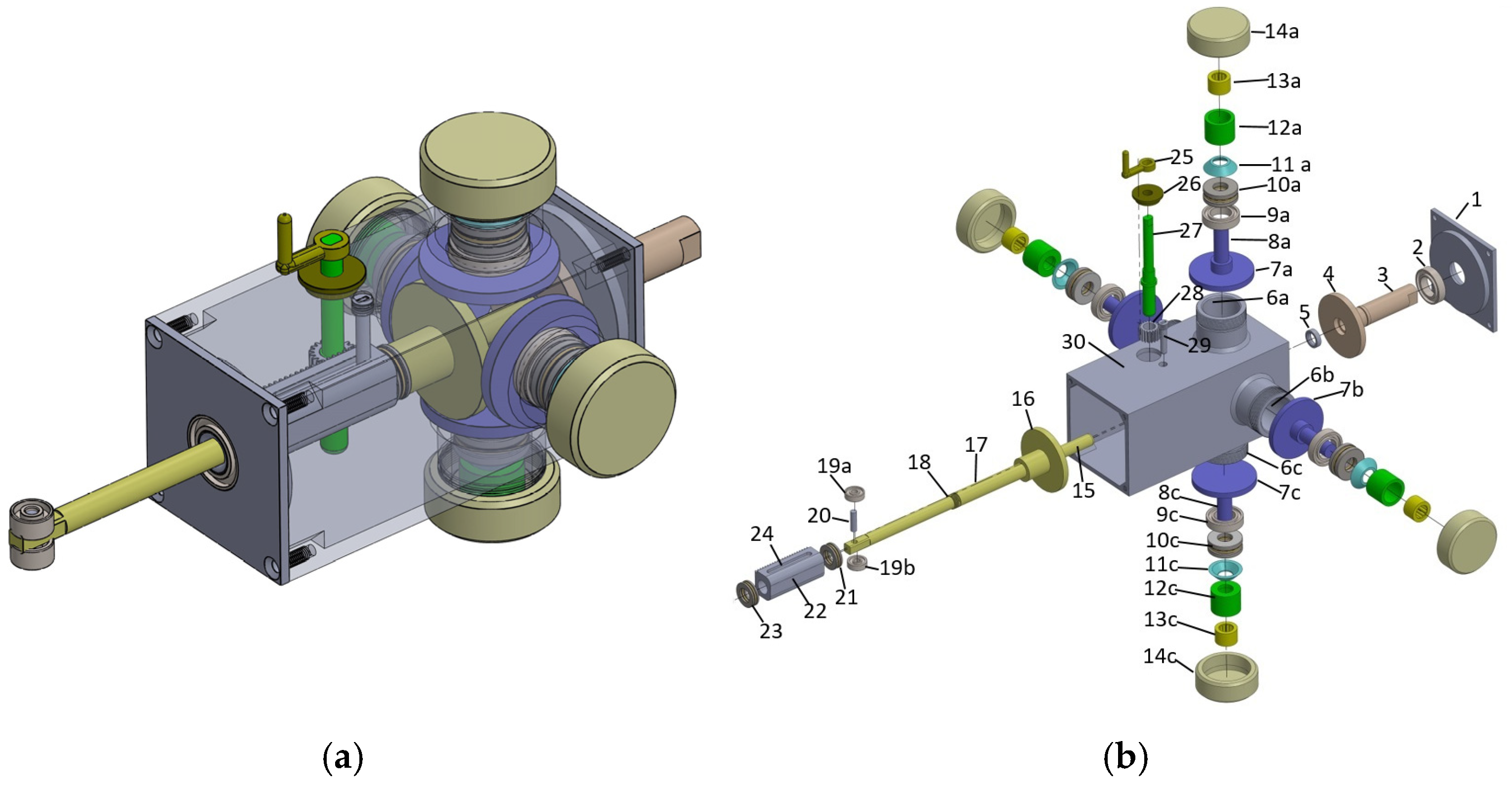
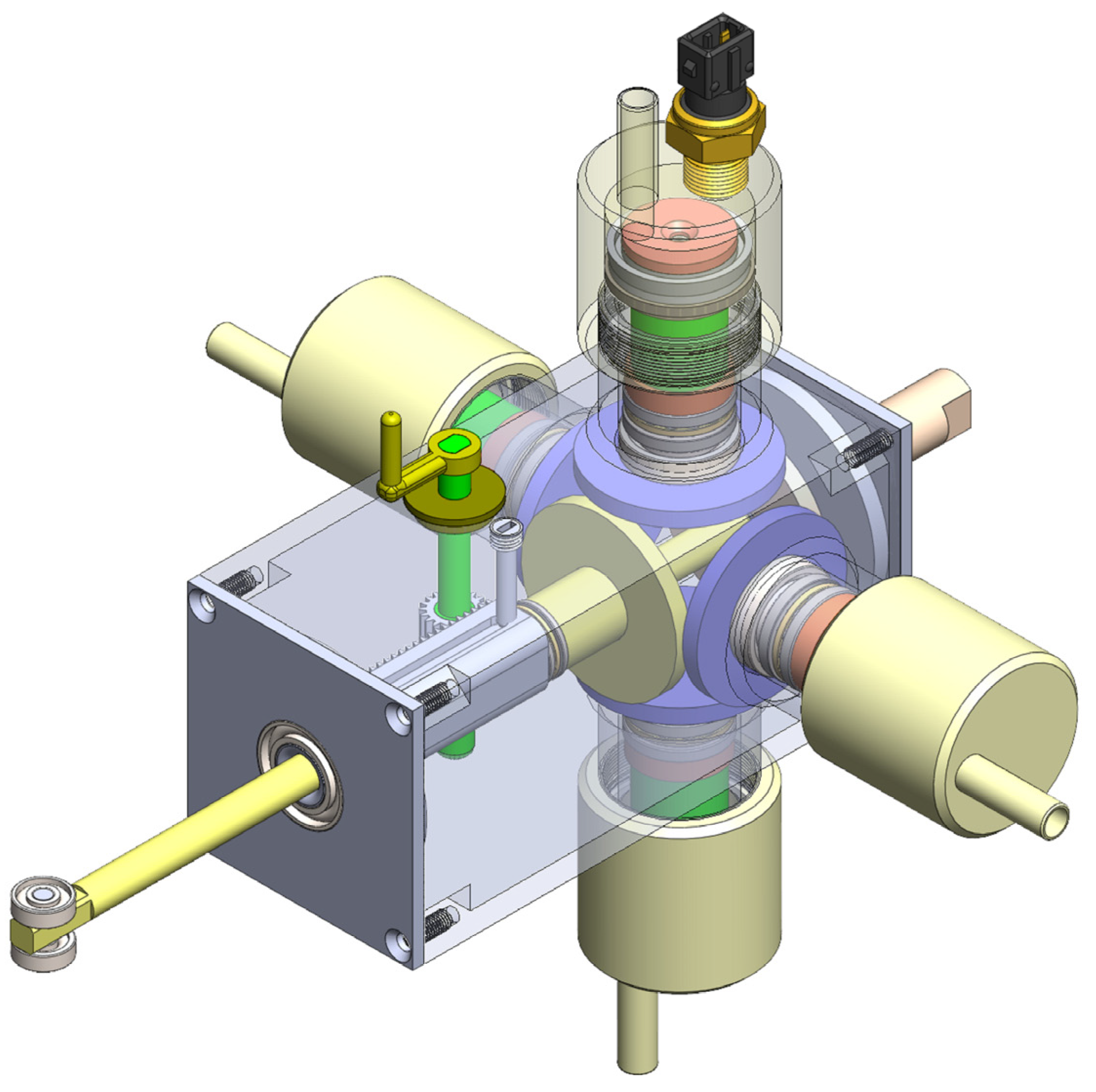
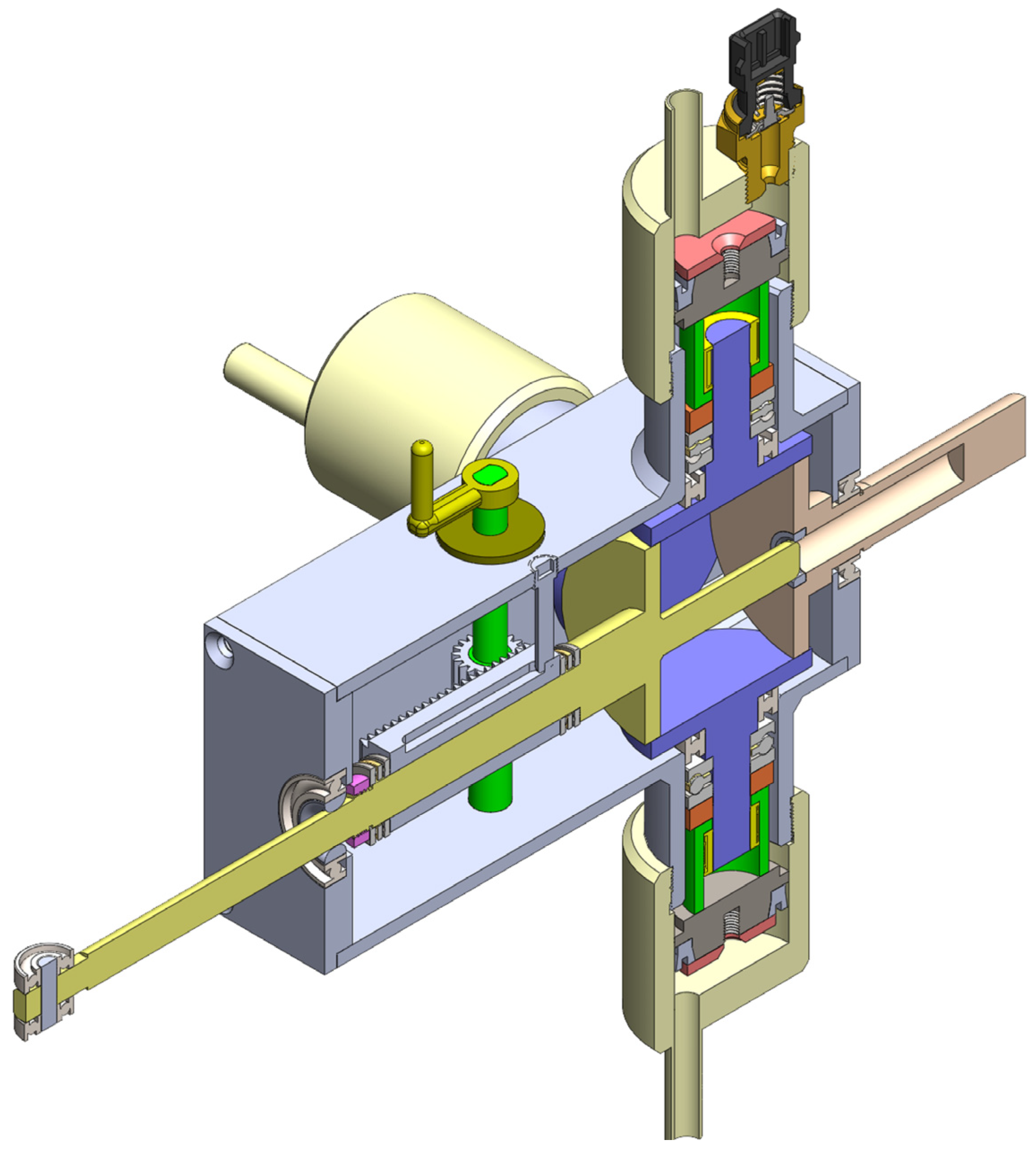
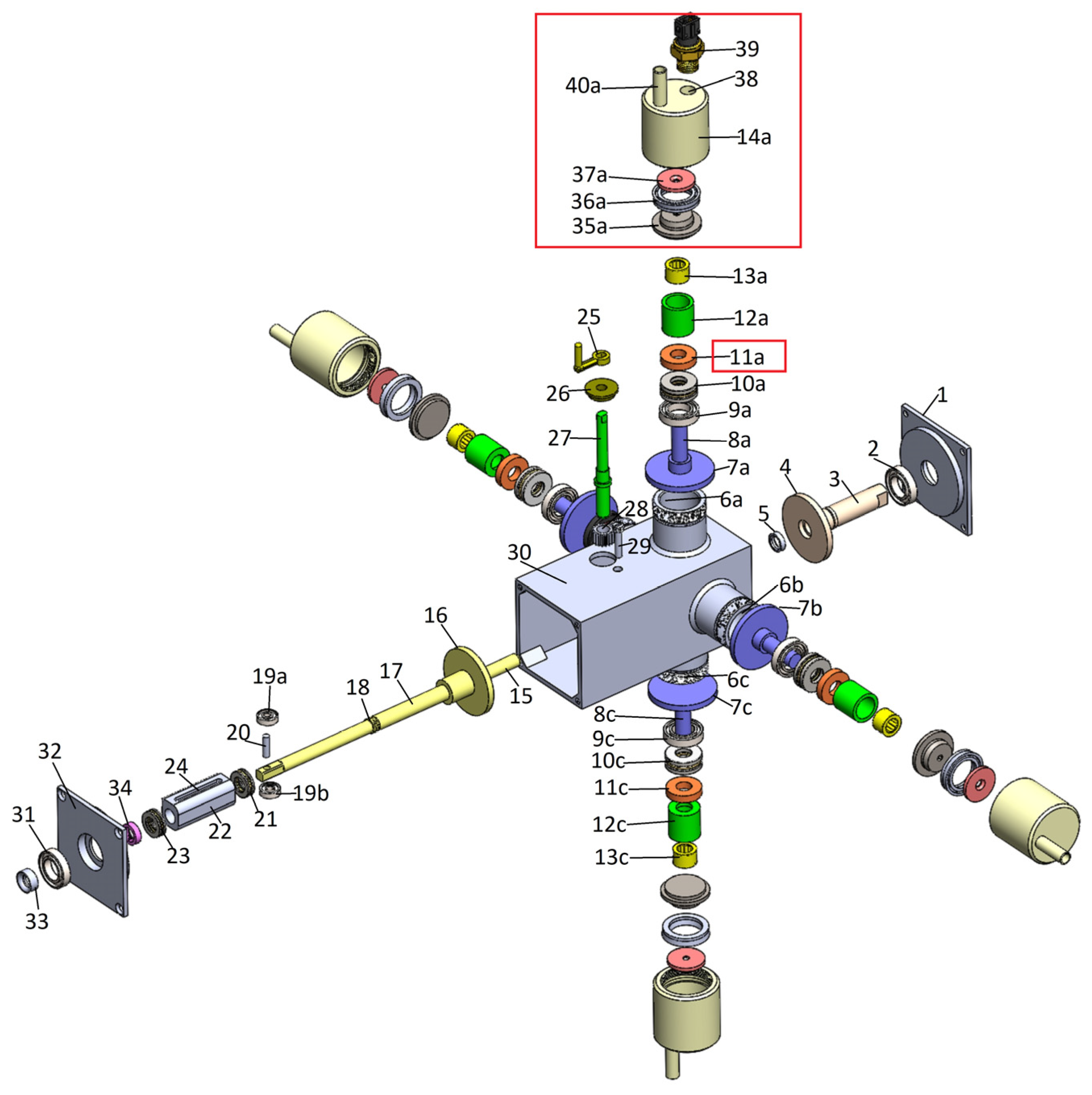
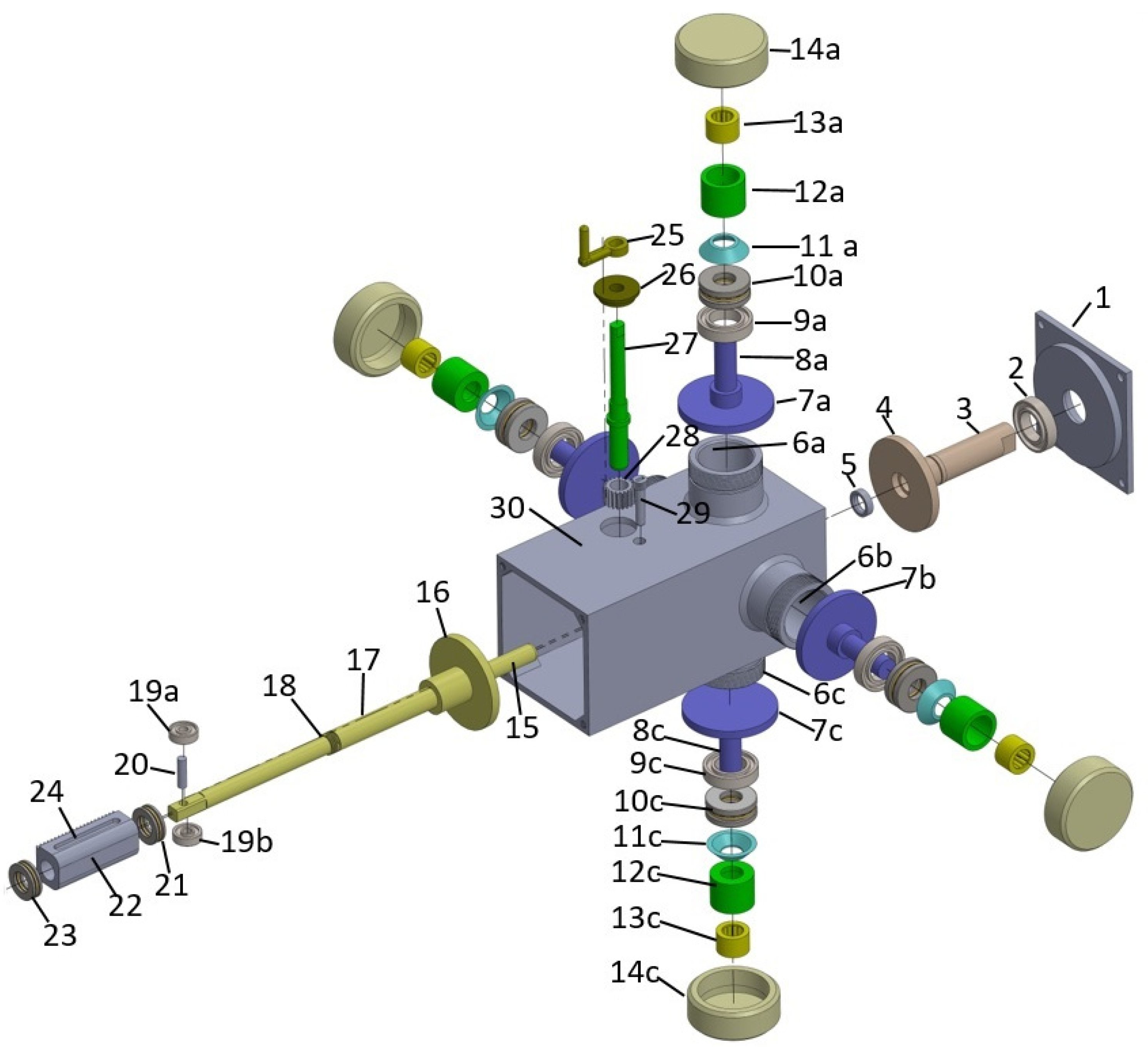
2.3.2. Three-Dimensional Model of the Proposed CAD CVT-II
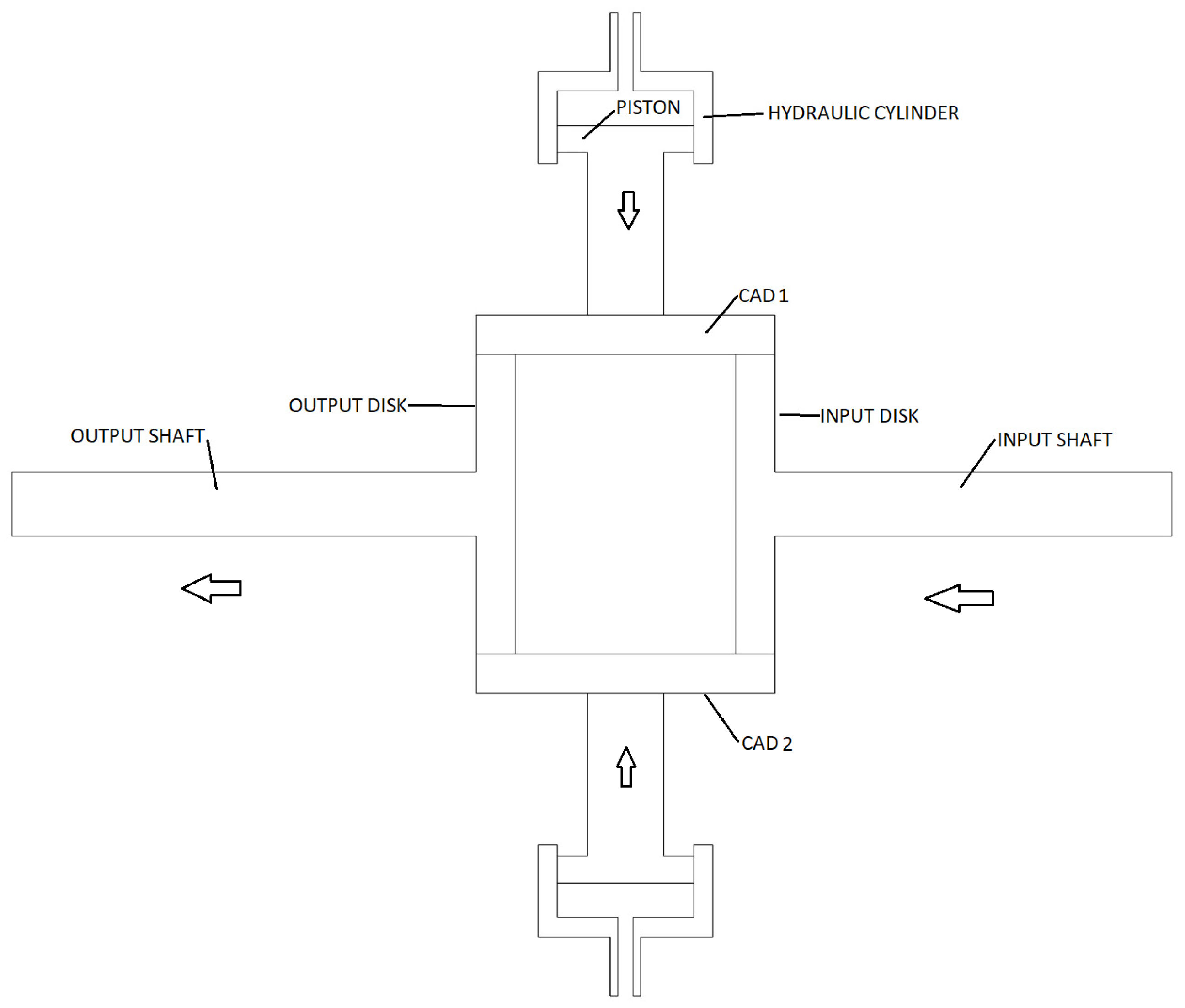
2.3.3. Configuration of the Proposed CAD CVT-II
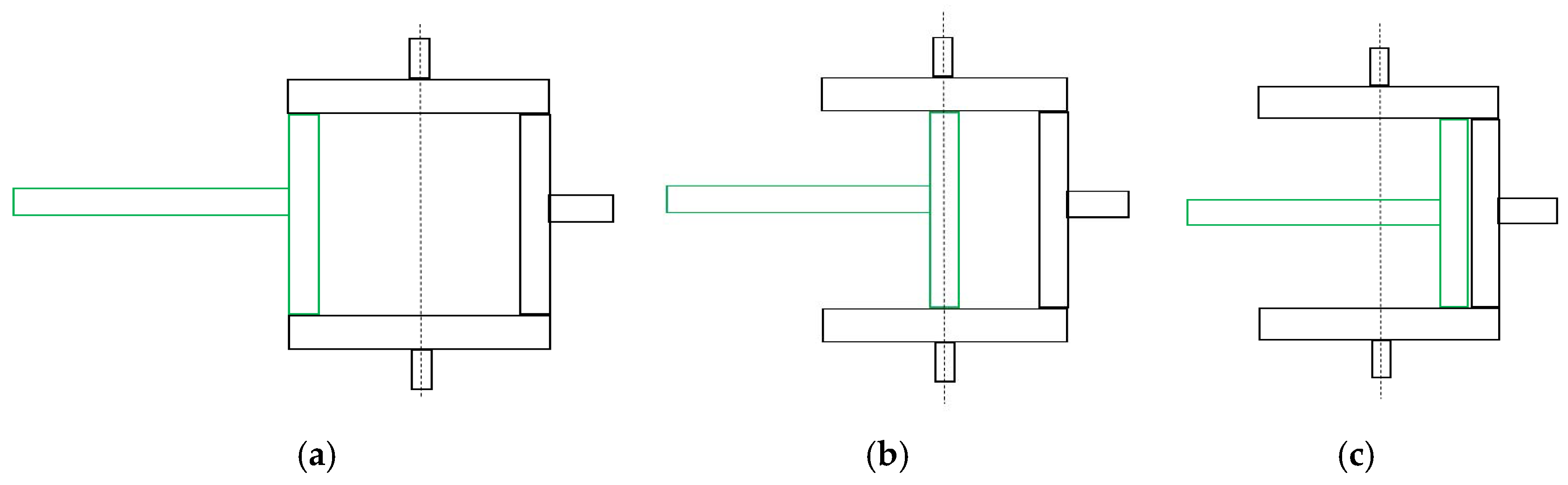
2.3.4. Operating Principle of the Proposed CAD CVT-II
2.4. Analysis of CAD CVT-II During Variable Torque
2.5. Design of Control System for CAD CVT-II
- A hydraulic actuation system to control hydraulic pressure in the cylinders of CAD CVT-II. Consequently, the force on traction disks can be regulated.
- A dynamic torque sensor must be attached to the CVT’s output. Consequently, the instantaneous required torque can be measured.
- Pressure sensors in the secondary cylinders (at least one). Consequently, any fluid leakage is detected.
2.5.1. Design of Energy-Efficient Hydraulic Actuation System
- The hydraulic actuation system motor must run only when a change in torque is required.
- The position of the motor can precisely control the pressure. Consequently, pressure acts as a function of the position of the motor.
- The motor must maintain its position during the off state to conserve energy.
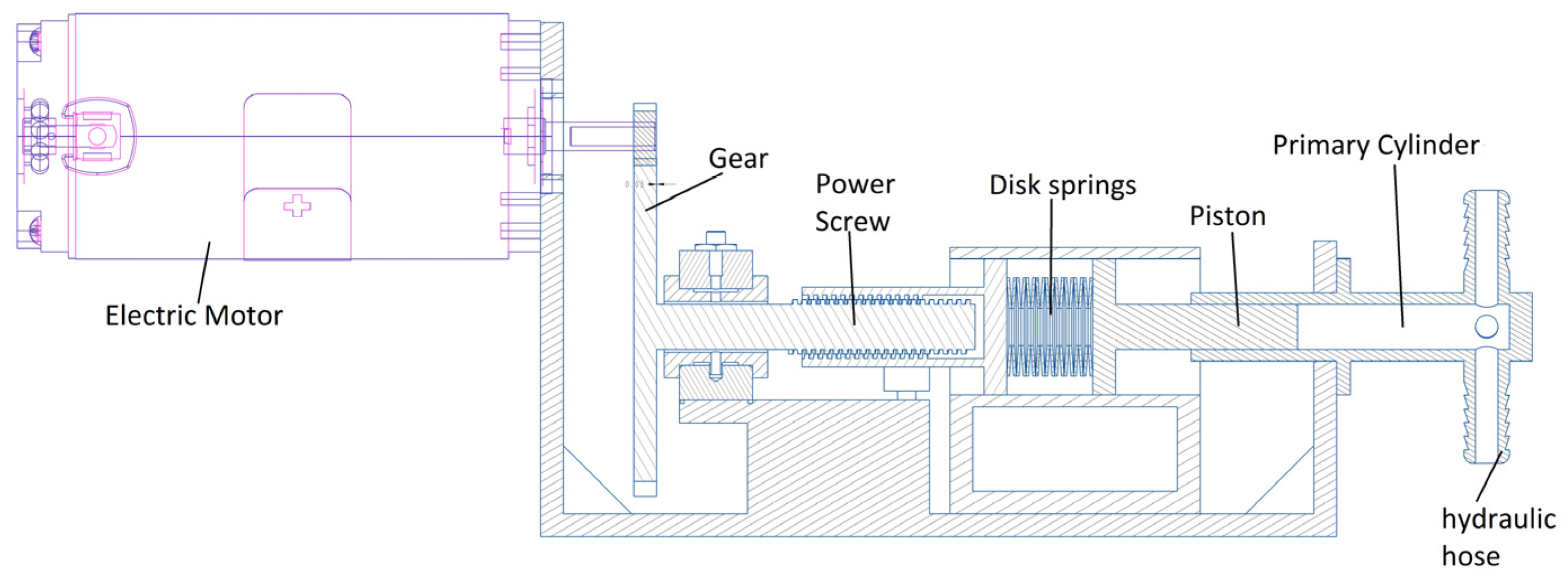
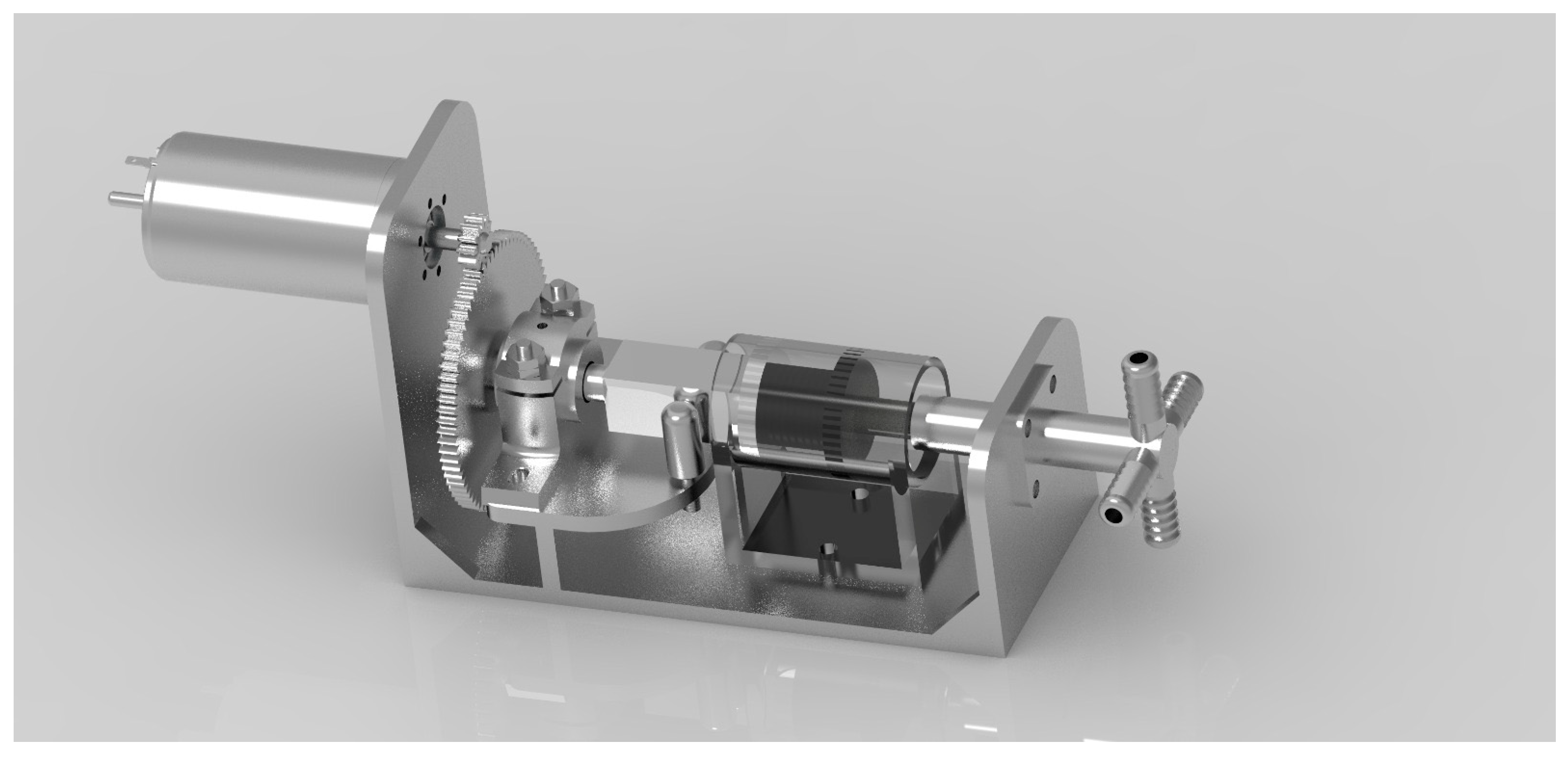
2.5.2. Three-Dimensional Model of Energy-Efficient Hydraulic Actuation System
2.5.3. Working Principle of the Energy-Efficient Hydraulic Actuation System
2.6. Analysis of the Control System of CAD CVT-II
2.6.1. Overview
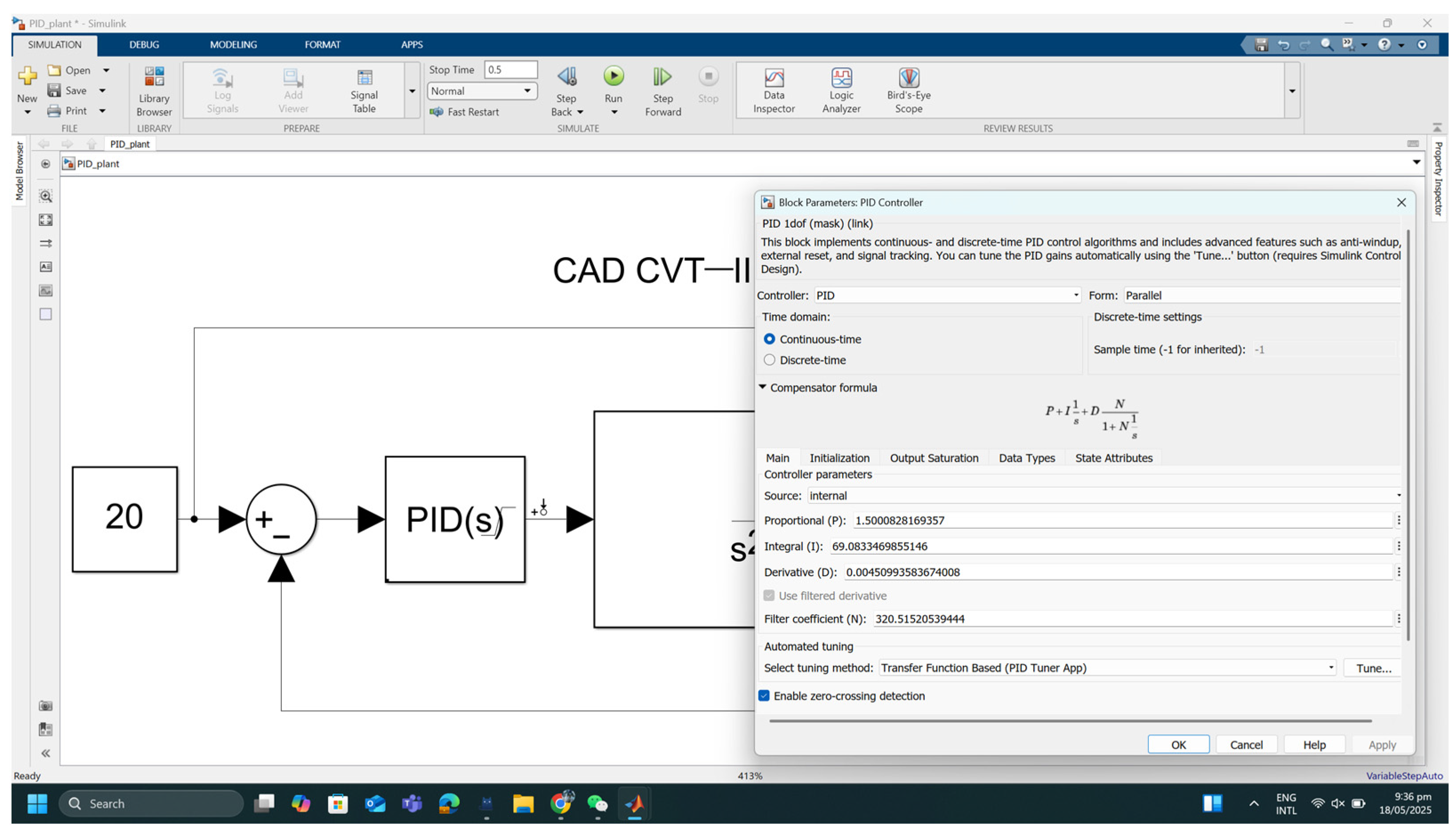
2.6.2. Transfer Function of Control System
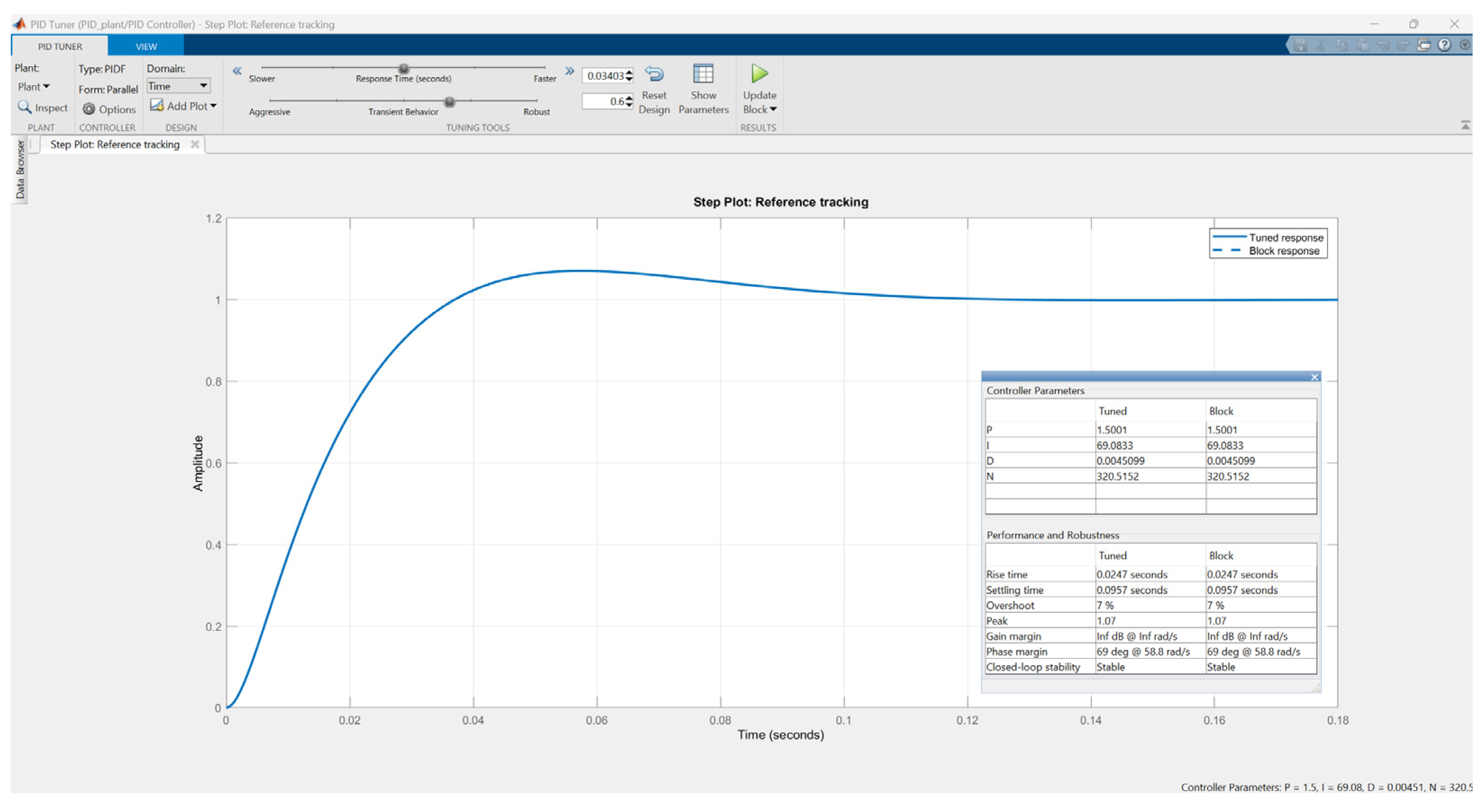
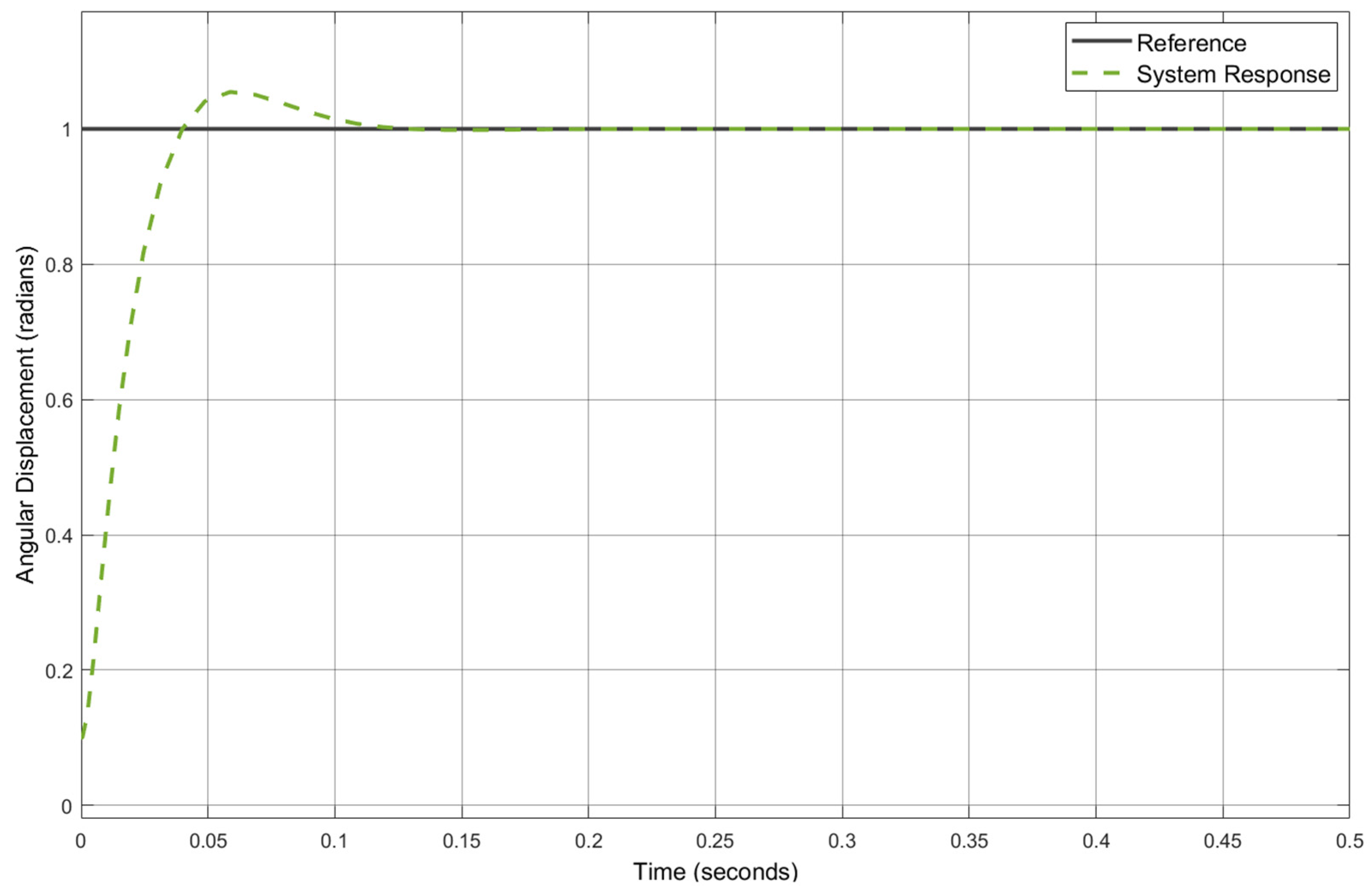
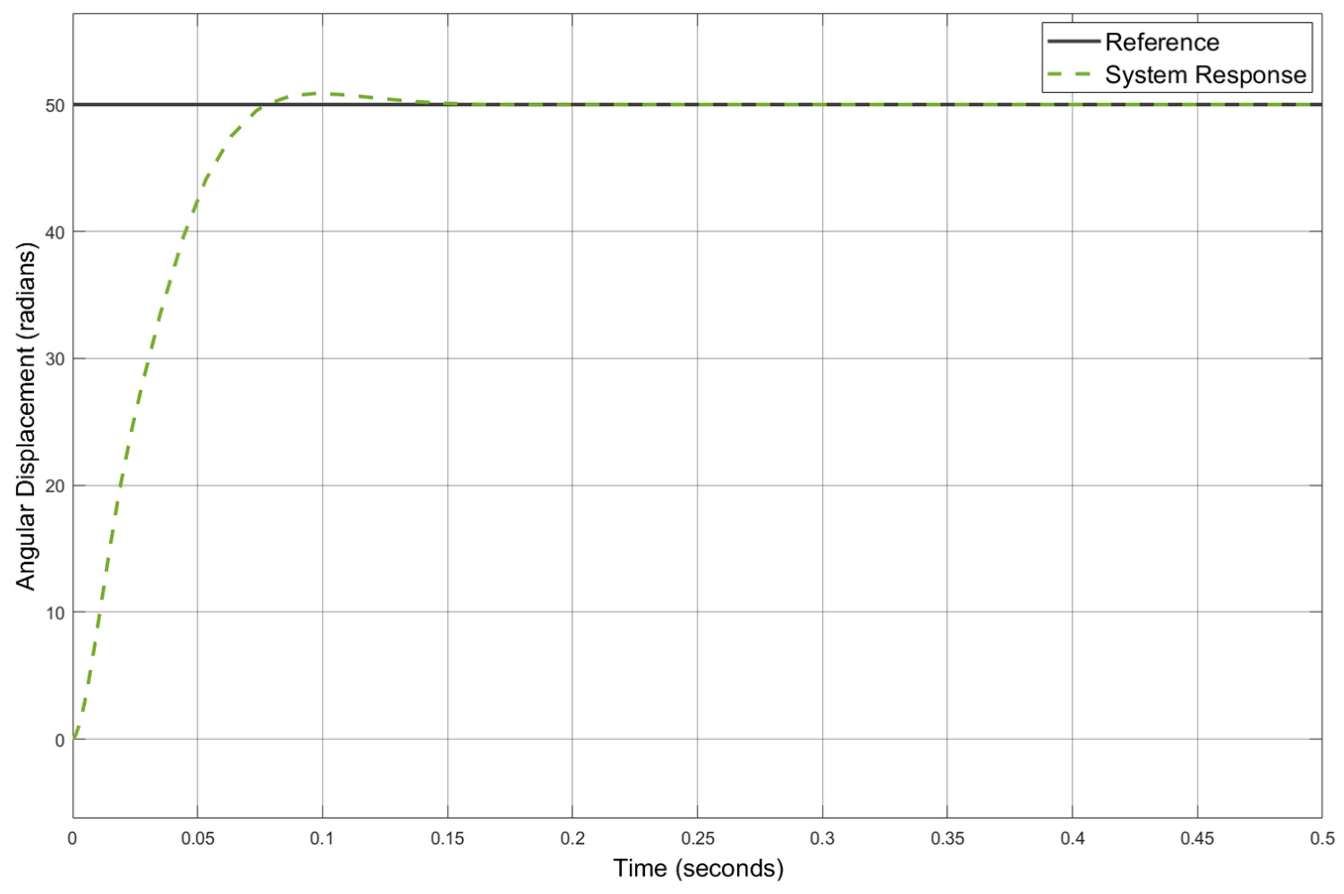
2.6.3. Control System Dynamic Response Evaluation
- I.
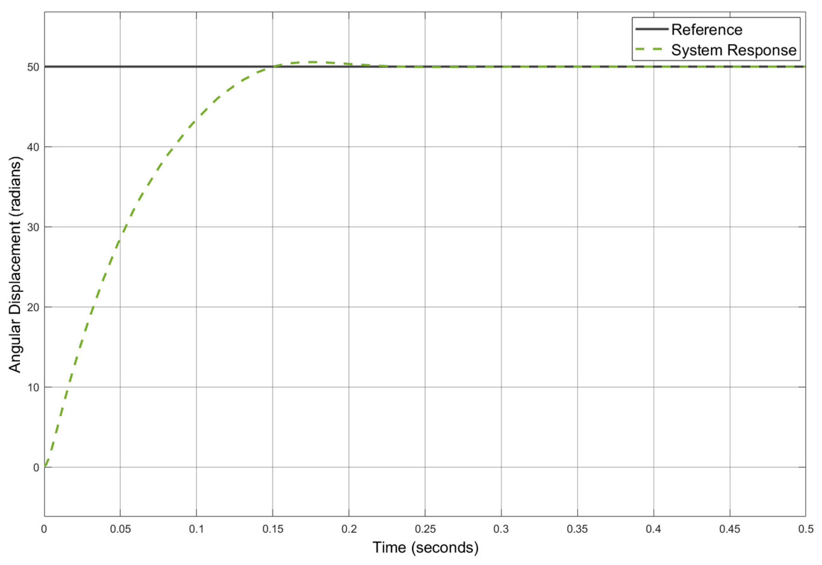
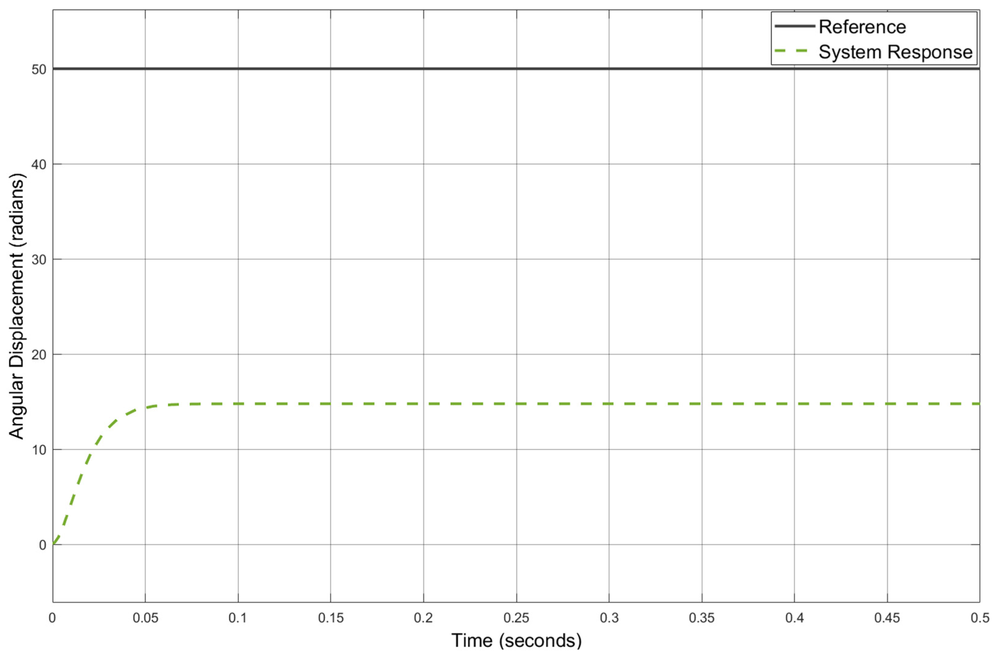
- Analysis of System Response to PID Controller
- II.
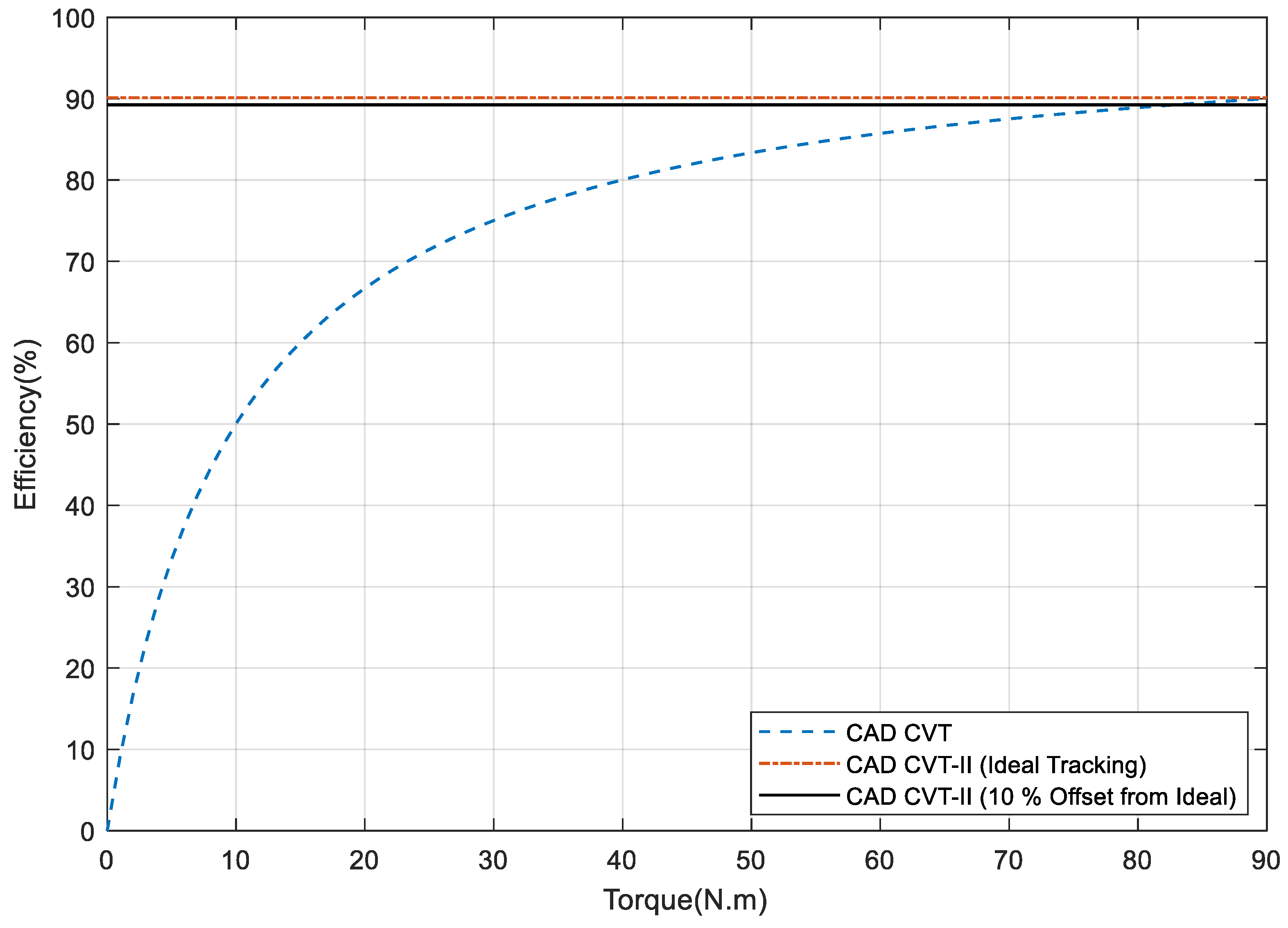
- Effect of Tracking Error on Energy Efficiency
- III.
- Tracking Strategy
2.7. Comparison with Current Commercial CVTs
3. Results and Discussion
4. Conclusions and Future Work
- Analyses of CAD CVT efficiency during variable-torque applications were performed. During analyses of the CAD CVT, it was observed that it has low energy efficiency in low torque regions.
- An improved mechanical design of a CAD CVT that is maximally efficient throughout its operating range was proposed. The new CVT was named CAD CVT-II.
- In CAD CVT-II, the force on the circumferentially arranged disks can be varied according to instantaneous torque requirements, thus resulting in improved efficiency in the low torque region.
- A hydraulic-actuation-based control system has been designed to provide control of CAD CVT-II. The novel features of the control system are as follows:
- There is almost negligible fluid movement in the hydraulic actuation system, which improves energy efficiency.
- The hydraulic actuation system has a self-locking capability, due to which it can be operated only when required; otherwise, it remains off. This also improves its energy efficiency.
- The proposed control system of CAD CVT-II can be controlled by a PID controller and is highly responsive.
Author Contributions
Funding
Data Availability Statement
Conflicts of Interest
Appendix A. Design of Energy-Efficient Hydraulic Actuation System
Appendix A.1. Development of Design Criteria
Appendix A.1.1. Problem Statement
- Consumes energy when a pressure change is required. Otherwise, it remains off and does not consume energy.
- Has a fast response time.
- Acts as a torque-to-force converter.
- Acts as a torque-to-force amplifier. That is, it should be able to produce a very high force with a motor with a very low torque.
- Is able to vary pressure and hence force throughout its range, even when the secondary piston has no movement.
- Does not move the hydraulic fluid to reduce energy losses. It should merely act as a force transfer medium.
Appendix A.1.2. Design Features of Hydraulic Actuation System
- I.
- Simple power screw
- It maintains its position when the electric motor is off. This enables the motor to remain off when there is no torque change.
- It provides a very high mechanical advantage, which enables us to drive the mechanism using an electric motor with very low torque and low power.
- II.
- Disk Springs
- III.
- Spur Gears
- IV.
- Disk Spring Placement
- In the original CAD CVT, a single disk spring is placed immediately behind each CAD. If we do not disturb the original design of the CAD CVT, then we will have two sets of disk springs, one inside the CVT and one inside the hydraulic actuation system. This arrangement results in the movement of hydraulic fluid entrapped between two sets of disk springs. Unlike traditional systems used for brake or clutch actuation, hydraulic fluid should not move in the desired system.
- If we remove disk springs from the hydraulic actuation system, we lose the ability to optimize accuracy and response time. Moreover, the problem of fluid movement will persist.
- If we place the disk springs of the hydraulic actuation system along with the disk spring of the CAD CVT, then the ability to optimize the response time and accuracy is maintained. However, the fluid movement persists.
- If we only remove the disk spring from the CAD CVT and replace it with a solid metallic bush, the fluid movement will stop. Moreover, the ability to optimize response time and accuracy is maintained.
Appendix B. Control System Mathematical Modeling
Appendix B.1. Power Screw Equations
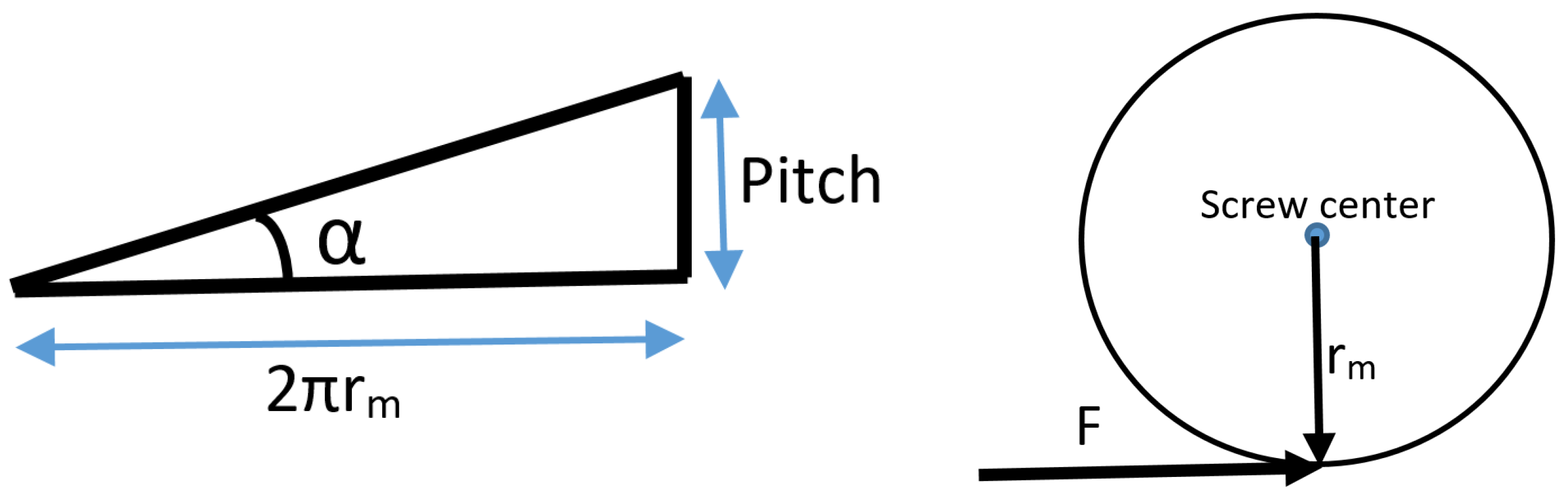
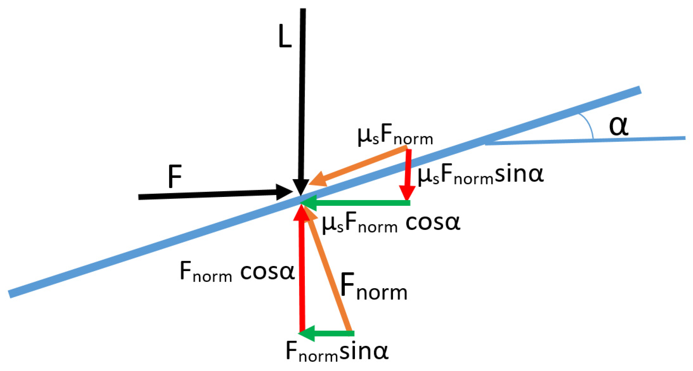
Appendix B.2. Torque Requirement of Power Screw
- The hydraulic fluid is incompressible.
- The hydraulic fluid is transmitted from the primary cylinder to the secondary cylinders through steel pipes so that volumetric variation in the steel hoses and the primary and secondary cylinders can be assumed to be negligible.
Appendix B.3. Torque Requirement of Motor
Appendix B.4. Transfer Function

| Parameter | Value | Parameter | Value |
|---|---|---|---|
| Pitch | 2 mm | J2 | kg m2 |
| rm | 5.5 mm | b2 | Nm/rad/s |
| α | k | Nm/A | |
| Kp | m/rad | Lind | H |
| Kg | R | 0.299 Ω | |
| Ks | 1,117,777 N/m | J1 | kg m2 |
| b3 | N/m/s | μs | 0.15 |
| m3 | 0.94 kg | b1 | Nm/rad/s |
Appendix C. Torque vs. Pressure
| Parameter | Value/Range |
|---|---|
| CAD CVT-II torque range | 0 to 90 Nm |
| Diameter of secondary cylinders | 36 mm |
| Pressure range | 0 to 50 Bar |
| Range of force on traction disks | 0 to 5 KN |
| Traction disks’ contact length | 2 mm |
| Traction disks’ stress at the contact point | 1.3 GPa |
| Traction disks’ material | SS 304 |
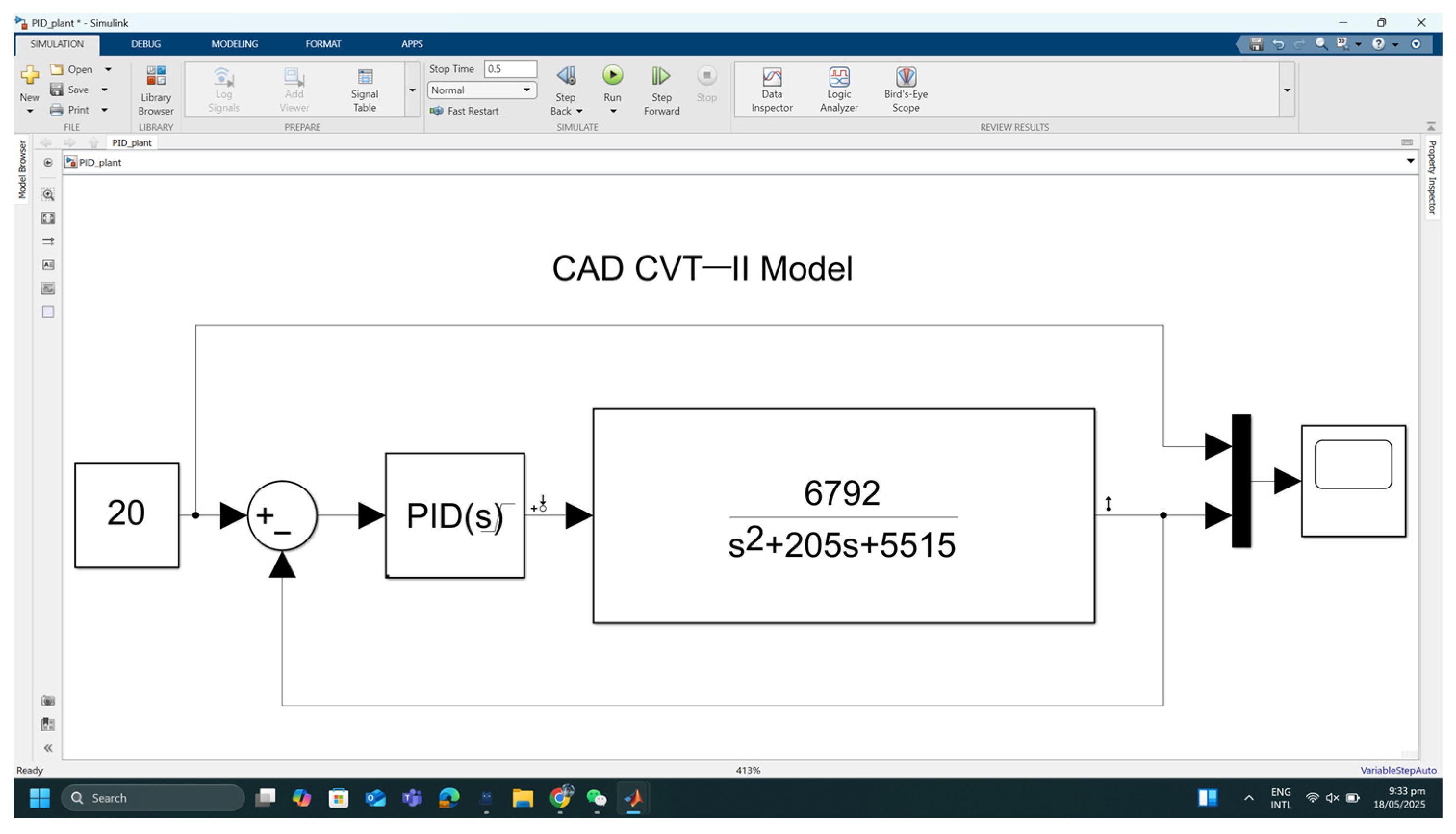
Appendix D. SIMULINK Model of CAD CVT-II PID Controller
References
- Carbone, G.; Mangialardi, L.; Mantriota, G. A Comparison of the Performances of Full and Half Toroidal Traction Drives. Mech. Mach. Theory 2004, 39, 921–942. [Google Scholar] [CrossRef]
- Kim, J.; Park, F.C.; Park, Y. Design, Analysis and Control of a Wheeled Mobile Robot with a Nonholonomic Spherical CVT. Int. J. Rob. Res. 2002, 21, 409–426. [Google Scholar] [CrossRef]
- Sheng, Y.; Escobar-Naranjo, D.; Stelson, K.A. Feasibility of Hydrostatic Transmission in Community Wind Turbines. Actuators 2023, 12, 426. [Google Scholar] [CrossRef]
- Cotrell, J. Assessing the Potential of a Mechanical Continuously Variable Transmission for Wind Turbines; National Renewable Energy Lab. (NREL): Golden, CO, USA, 2005.
- Nguyen, V.H.; Do, T.C.; Ahn, K.K. Investigation and Optimization of Energy Consumption for Hybrid Hydraulic Excavator with an Innovative Powertrain. Actuators 2023, 12, 382. [Google Scholar] [CrossRef]
- Jawad, Q.A.; Ali, A.K. Comparison of CVT Performance with the Manual and Automatic Transmission for Evaluation the Fuel Consumption and Exhaust Emissions. Basrah J. Eng. Sci. 2020, 20, 15–22. [Google Scholar] [CrossRef]
- Ruan, J.; Walker, P.D.; Wu, J.; Zhang, N.; Zhang, B. Development of Continuously Variable Transmission and Multi-Speed Dual-Clutch Transmission for Pure Electric Vehicle. Adv. Mech. Eng. 2018, 10, 1–15. [Google Scholar] [CrossRef]
- Mobedi, E.; Ismet, M.C.D. A Continuously Variable Transmission System Designed for Human-Robot Interfaces. In Proceedings of the Asian MMS Conference; Springer Nature: Berlin, Germany, 2018. [Google Scholar]
- Mobedi, E.; Dede, M.İ.C. Geometrical Analysis of a Continuously Variable Transmission System Designed for Human-Robot Interfaces. Mech. Mach. Theory 2019, 140, 567–585. [Google Scholar] [CrossRef]
- Jin, Y.; Liu, J.; Xu, Z.; Yuan, S.; Li, P.; Wang, J. Development Status and Trend of Agricultural Robot Technology. Int. J. Agric. Biol. Eng. 2021, 14, 1–19. [Google Scholar] [CrossRef]
- Micklem, J.D.; Longmore, D.K.; Burrows, C.R. Modelling of the Steel Pushing V-Belt Continuously Variable Transmission. Proc. Inst. Mech. Eng. Part C J. Mech. Eng. Sci. 1994, 208, 13–27. [Google Scholar] [CrossRef]
- Lin, X.; Peng, Y.; Hong, R.; Wang, Y. Research on a Novel Discrete Adjustable Radiuses Type Continuously Variable Transmission. Meccanica 2022, 57, 1155–1171. [Google Scholar] [CrossRef]
- Verbelen, F.; Haemers, M.; De Viaene, J.; Derammelaere, S.; Stockman, K.; Sergeant, P. Adaptive PI Controller for Slip Controlled Belt Continuously Variable Transmission. IFAC-PapersOnLine 2018, 51, 101–106. [Google Scholar] [CrossRef]
- Kim, T.; Kim, H. Low-Level Control of Metal Belt CVT Considering Shift Dynamics and Ratio Valve On-off Characteristics. KSME Int. J. 2000, 14, 645–654. [Google Scholar] [CrossRef]
- Guang-bin, W.; Yan-hui, L.; Xiao-wei, X. Optimization of CVT Efficiency Based on Clamping Force Control. IFAC-PapersOnLine Conf. Pap. Arch. 2018, 51, 898–903. [Google Scholar] [CrossRef]
- Pulles, R.J.; Bonsen, B.; Veenhuizen, P.A.; Steinbuch, M. Slip Controller Design and Implementation in a Continuously Variable Transmission. In Proceedings of the American Control Conference, Portland, OR, USA, 8–10 June 2005; SAE International: Warrendale, PA, USA, 2005. [Google Scholar]
- Ye, M.; Liu, Y.G.; Cheng, Y. Modeling and Ratio Control of an Electromechanical Continuously Variable Transmission. Int. J. Automot. Technol. 2016, 17, 225–235. [Google Scholar] [CrossRef]
- Chen, T.; Xu, X.; Cai, Y.; Chen, L.; Li, K. QPSOMPC-Based Chassis Coordination Control of 6WIDAGV for Vehicle Stability and Trajectory Tracking. J. Frankl. Inst. 2025, 362, 107458. [Google Scholar] [CrossRef]
- Zhao, J.; Li, R.; Zheng, X.; Li, W.; Hu, C.; Liang, Z.; Wong, P.K. Constrained Fractional-Order Model Predictive Control for Robust Path Following of FWID-AGVs with Asymptotic Prescribed Performance. IEEE Trans. Veh. Technol. 2025, 74, 2692–2705. [Google Scholar] [CrossRef]
- Chen, T.; Cai, Y.; Chen, L.; Xu, X. Trajectory and Velocity Planning Method of Emergency Rescue Vehicle Based on Segmented Three-Dimensional Quartic Bezier Curve. IEEE Trans. Intell. Transp. Syst. 2023, 24, 3461–3475. [Google Scholar] [CrossRef]
- Liu, H.; Yan, S.; Shen, Y.; Li, C.; Zhang, Y.; Hussain, F. Model Predictive Control System Based on Direct Yaw Moment Control for 4wid Self-Steering Agriculture Vehicle. Int. J. Agric. Biol. Eng. 2021, 14, 175–181. [Google Scholar] [CrossRef]
- Li, J.; Wu, Z.; Li, M.; Shang, Z. Dynamic Measurement Method for Steering Wheel Angle of Autonomous Agricultural Vehicles. Agriculture 2024, 14, 1602. [Google Scholar] [CrossRef]
- Xu, G.; Fang, H.; Song, Y.; Du, W. Optimal Design and Analysis of Cavitating Law for Well-Cellar Cavitating Mechanism Based on MBD-DEM Bidirectional Coupling Model. Agriculture 2023, 13, 142. [Google Scholar] [CrossRef]
- Fu, W.; Lu, W.; Liu, H.; Yuan, X.; Zeng, D. Smooth Braking Control of Excavator Hydraulic Load Based on Command Reshaping. ISA Trans. 2025, 158, 674–685. [Google Scholar] [CrossRef] [PubMed]
- Shi, B.; Xiong, L.; Yu, Z. Pressure Estimation of the Electro-Hydraulic Brake System Based on Signal Fusion. Actuators 2021, 10, 240. [Google Scholar] [CrossRef]
- Shi, Q.; He, L. A Model Predictive Control Approach for Electro-Hydraulic Braking by Wire. IEEE Trans. Ind. Inform. 2023, 19, 1380–1388. [Google Scholar] [CrossRef]
- Chen, X.; Hang, P.; Wang, W.; Li, Y. Design and Analysis of a Novel Wheel Type Continuously Variable Transmission. Mech. Mach. Theory 2017, 107, 13–26. [Google Scholar] [CrossRef]
- Kazerounian, K.; Furu-Szekely, Z. Parallel Disk Continuously Variable Transmission (PDCVT). Mech. Mach. Theory 2006, 41, 537–566. [Google Scholar] [CrossRef]
- KOMATSUBARA, H.; KURIBAYASHI, S. Research and Development of Cone to Cone Type CVT (1st Report, Fundamental Structure, Speed Change Mechanism and Design of CTC-CVT). Trans. JSME 2017, 83, 16-00477. (In Japanese) [Google Scholar] [CrossRef]
- Carter, J. The Design and Analysis of an Alternative Traction Drive CVT. In Proceedings of the SAE 2003 World Congress & Exhibition, Detroit, MI, USA, 3–6 March 2003. [Google Scholar]
- Shen, C.J.; Yuan, S.H.; Hu, J.B.; Wu, W.; Wei, C.; Chen, X. Principle and Characteristics of Original Hydraulic Traction Drive CVT. J. Cent. South Univ. 2014, 21, 1654–1659. [Google Scholar] [CrossRef]
- Ghariblu, H.; Behroozirad, A.; Madandar, A. Traction and Efficiency Performance of Ball Type CVTs. Int. J. Automot. Eng. 2014, 4, 738–748. [Google Scholar]
- Li, C.; Li, H.; Li, Q.; Zhang, S.; Yao, J. Modeling, Kinematics and Traction Performance of No-Spin Mechanism Based on Roller-Disk Type of Traction Drive Continuously Variable Transmission. Mech. Mach. Theory 2019, 133, 278–294. [Google Scholar] [CrossRef]
- Drescher, D.; Naves, M.; de Vries, T.J.A.; Buijze, M.; Stramigioli, S. Power Split Based Dual Hemispherical Continuously Variable Transmission. Actuators 2017, 6, 15. [Google Scholar] [CrossRef]
- Kim, J.; Park, F.C.; Park, Y.; Shizuo, M. Design and Analysis of a Spherical Continuously Variable Transmission. J. Mech. Des. 2002, 124, 21–29. [Google Scholar] [CrossRef]
- Tomaselli, M.; Bottiglione, F.; Lino, P.; Carbone, G. NuVinci Drive: Modeling and Performance Analysis. Mech. Mach. Theory 2020, 150, 103877. [Google Scholar] [CrossRef]
- Verbelen, F.; Derammelaere, S.; Sergeant, P.; Stockman, K. Half Toroidal Continuously Variable Transmission: Trade-off between Dynamics of Ratio Variation and Efficiency. Mech. Mach. Theory 2017, 107, 183–196. [Google Scholar] [CrossRef]
- Delkhosh, M.; Foumani, M.S. Multi-Objective Geometrical Optimization of Full Toroidal CVT. Int. J. Automot. Technol. 2013, 14, 707–715. [Google Scholar] [CrossRef]
- Bilal, M.; Zhu, Q.; Qureshi, S.R.; Elahi, A.; Nadeem, M.K.; Khan, S. A Novel Continuously Variable Transmission with Circumferentially Arranged Disks (CAD CVT). Actuators 2024, 13, 208. [Google Scholar] [CrossRef]
- Available online: www.maxongroup.com (accessed on 1 December 2024).


| Parameter | Value | Parameter | Value |
|---|---|---|---|
| Fn | 5000 N | n | 4 |
| 0.42 | a | 0.001 m | |
| 0.002 | 0.025 m | ||
| 0.35 | 0.0085 m | ||
| 0.001 | 0.005 m | ||
| 0.002 | 0.006 m | ||
| 0.001 | 0.0085 m | ||
| 0.026 m | 0.0275 m | ||
| 0.025 m | 0.001861 | ||
| 0.0004475 | 9.308 |
| S. No. | Part No. | Description |
|---|---|---|
| 1 | ‘1’ | Cover on the input side of the CVT. |
| 2 | ‘2’ | A ball bearing that supports the input shaft. |
| 3 | ‘3’ | The shaft of the CVT that receives input from the motor/engine. |
| 4 | ‘4’ | The disk is connected to shaft ‘3’ for delivering motion to traction disks (circumferentially arranged disks). |
| 5 | ‘5’ | A hybrid bearing that simultaneously supports the linear and rotary motion of shaft ‘15’ so that shaft ‘15’ and shaft ‘3’ remain aligned, resulting in the alignment of disk ‘4’ and disk ‘16’. |
| 6 | ‘6a’, ‘6b’ ‘6c’, ‘6d’ | Casings/housings for traction disks. |
| 7 | ‘7a’, ‘7b’, ‘7c’, ‘7d’ | Traction disks. They provide traction between input disk ‘4’ and output disk ’16’. |
| 8 | ‘8a’, ‘8b’, ‘8c’, ‘8d’ | Shafts of traction disks ‘7a’, ‘7b’, ‘7c’, ‘7d’. |
| 9 | ‘9a’, ‘9b’, ‘9c’, ‘9d’ | Ball bearings that provide alignment and support to the traction disks. |
| 10 | ‘10a’, ‘10b’, ‘10c’, ‘10d’ | Thrust bearings. (Their primary purpose is to enable traction disks to rotate smoothly while being axially pressed by a disk spring.) |
| 11 | ‘11a’, ‘11b’, ‘11c’, ‘11d’ | Disk springs in the CAD CVT. Simple metallic spacers in CAD CVT-II. |
| 12 | ‘12a’, ‘12b’, ‘12c’, ‘12d’ | Spacers. They provide two functions. Firstly, they transfer the axial load to ‘11a’, ‘11b’, ‘11c’, and ‘11d’. Secondly, they act as housings for pin bearings ‘13a’, ‘13b’, ‘13c’, and ‘13d’. |
| 13 | ‘13a’, ‘13b’, ‘13c’, ‘13d’ | Pin bearings. They, along with ball bearings ‘9a’, ‘9b’, ‘9c’, and ‘9d’, align traction disks and enable their smooth rotation. |
| 14 | ‘14a’, ‘14b’, ‘14c’, ‘14d’ | Secondary cylinders that support the movement of pistons ‘35a’, ‘35b’, ‘35c’, and ’35d’, respectively. The hydraulic pressure inside these cylinders determines the force applied to traction disks. An increase in force on traction disks increases the tractive force between traction disks and input disk ‘4′ and output disk ‘16′. This component of CAD CVT-II is different from the CAD CVT [39]. |
| 15 | ‘15’ | Its essential purpose is to provide support and alignment to the output shaft, enabling it to remain aligned during its simultaneous rotary and linear movement. Shaft ‘15’ is fitted in bearing ‘5’. |
| 16 | ‘16’ | Output disk. It is attached to output shaft ‘17’ and has traction contact with circumferentially arranged disks. It transfers motion from circumferentially arranged disks (traction disks) to the output shaft. The location of the traction contact between the output disk and traction disks governs the gear ratio. |
| 17 | ‘17’ | Output shaft. |
| 18 | ‘18’ | Threads on the output shaft for retaining axial movement of rack ‘22’. |
| 19 | ‘19a’, ‘19b’ | These are roller bearings that will slide in a hollow shaft that is square from the inside. The hollow shaft in which these roller bearings will slide will be the input shaft of the load driven by the CVT. When the output shaft is moved axially during changes in gear ratios, these bearings help reduce friction between the CVT’s output shaft and the load’s input shaft. |
| 20 | ‘20’ | Pin supporting bearings ‘19a’ and ‘19b’. |
| 21 | ‘21’ | Thrust bearing between rack ‘22’ and output shaft ‘17’. This reduces the friction between rack ‘22’ and output shaft ‘17’ when the output shaft is axially pushed towards the input shaft during a gear ratio change. |
| 22 | ‘22’ | Rack. It is part of the rack-and-pinion mechanism, which moves the output shaft in the axial direction for a gear ratio change. |
| 23 | ‘23’ | Thrust bearing between rack ‘22’ and output shaft ‘17’. This reduces friction between rack ‘22’ and output shaft ‘17’ when the output shaft is axially pushed away from the input shaft during a gear ratio change. |
| 24 | ‘24’ | Guiding slot in rack ‘22’. This restricts the movement of the rack to the axial direction only. |
| 25 | ‘25’ | Handles the operating rack and pinion mechanism for a gear ratio change. |
| 26 | ‘26’ | Bush/bearing. |
| 27 | ‘27’ | Pinion shaft. |
| 28 | ‘28’ | A small spur gear that acts as a pinion. |
| 29 | ‘29’ | The guiding pin that sits in the guiding slot of the rack. |
| 30 | ‘30’ | CVT casing. |
| 31 | ‘31′ | Output shaft bearing. |
| 32 | ‘32’ | Cover on the output side of the CVT. |
| 33 | ‘33’ | Sliding bearing that supports the sliding movement of output shaft ‘17’. |
| 34 | ‘34’ | Nut for threads ‘18’. |
| 35 | ‘35a’, ‘35b’ ‘35c’, ‘35d’ | Pistons that are used to convert hydraulic pressure in secondary cylinders to force on traction disks. They are available in CAD CVT-II. However, they are not available in the CAD CVT [39]. |
| 36 | ‘36a’, ‘36b’ ‘36c’, ‘36d’ | Lip seals fitted to pistons ‘35a’, ‘35b’, ‘35c’, and ‘35d’, respectively, for stopping the leakage of hydraulic fluid. They are available in CAD CVT-II. However, they are not available in the CAD CVT [39]. |
| 37 | ‘37a’, ‘37b’ ‘37c’, ‘37d’ | Washers for the proper fixing of lip seals. They are available in CAD CVT-II. However, they are not available in CAD CVT [39]. |
| 38 | ‘38’ | Threaded hole for fixing pressure sensor ‘39’. It is available in CAD CVT-II. However, it is not available in the CAD CVT [39]. |
| 39 | ‘39’ | Pressure sensor. It is available in CAD CVT-II. However, it is not available in the CAD CVT [39]. |
| S. No. | Part No. | Description |
|---|---|---|
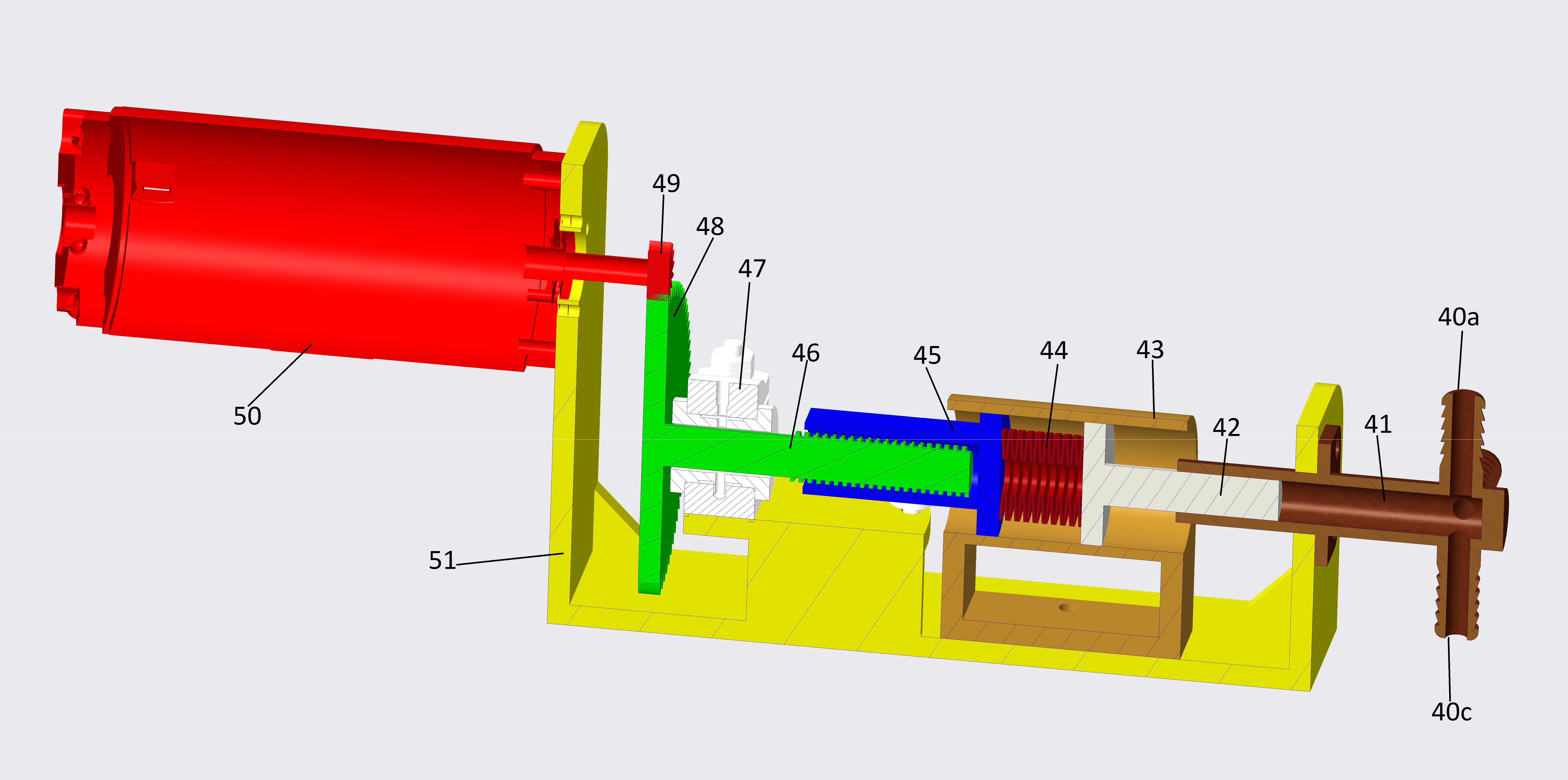
| 1 | ‘40a’, ‘40b’ ‘40c’, ‘40d’ | Steel pipes for transferring hydraulic fluid between secondary cylinders ‘14a’, ‘14b’, ‘14c’, ‘14d’ and primary cylinder ‘41’. |
| 2 | ‘41’ | Primary cylinder. It is part of the hydraulic actuation system. The pressure generated in the primary cylinder is transferred through hydraulic fluid to the secondary cylinders. |
| 3 | ‘42’ | The piston of primary cylinder ‘41’. This piston is pressed by the disk springs. |
| 4 | ‘43’ | Hollow cylinder for keeping piston ‘42’, disk springs ‘44’, and piston of power screw ‘45’ aligned. |
| 5 | ‘44’ | Disk springs. They transfer the force of power screw ‘45’ to the piston of primary cylinder ‘41’. |
| 6 | ‘45’ | Piston/nut of power screw. It can move linearly but cannot rotate. When the power screw is rotated by motor ‘50’, it moves linearly, resulting in compression of disk springs ‘44’, which in turn transfer the force to piston ‘42’. |
| 7 | ‘46’ | Power screw. |
| 8 | ‘47’ | Brackets for supporting power screw ‘46’. |
| 9 | ‘48’ | Gear attached to the power screw. |
| 10 | ‘49’ | Pinion attached to electric motor ‘50’. |
| 11 | ‘50’ | An electric motor that is used to drive the hydraulic actuation system of CAD CVT-II. |
| 12 | ‘51’ | Frame for supporting different components of CAD CVT-II. |
| Parameter | Value | Parameter | Value |
| Pitch | 2 mm | J2 | 20.057 × kg m2 |
| rm | 5.5 mm | b2 | 20.45 × Nm/rad/s |
| α | 3.312 | k | 3.02 × Nm/A |
| Kp | 3.183 × m/rad | Lind | 0.082 × H |
| Kg | R | 0.299 Ω | |
| Ks | 1,117,777 N/m | J1 | 143.95 × kg m2 |
| b3 | 1.434 × N/m/s | μs | 0.15 |
| m3 | 0.94 kg | b1 | 8.687 × Nm/rad/s |
| Qualitative Parameter | CAD CVT-II | CAD CVT | Push Belt CVT | Toroidal CVT |
|---|---|---|---|---|
| Direction reversal without requiring additional gears or clutches | Yes | Yes | No | No |
| Can be designed for very large torques such as trucks or trailers | Yes | Yes | No So far limited to cars only | No Increasing No. of toroids for increasing torque negatively affects the gear ratio range |
| Efficiency during variable-torque applications | High | Low | Low It can be improved through dynamic traction control; however, its implementation is difficult | Low It can be improved through dynamic traction control; however, its implementation is difficult |
| Commercial Availability | No | No | Yes | Yes |
Disclaimer/Publisher’s Note: The statements, opinions and data contained in all publications are solely those of the individual author(s) and contributor(s) and not of MDPI and/or the editor(s). MDPI and/or the editor(s) disclaim responsibility for any injury to people or property resulting from any ideas, methods, instructions or products referred to in the content. |
© 2025 by the authors. Licensee MDPI, Basel, Switzerland. This article is an open access article distributed under the terms and conditions of the Creative Commons Attribution (CC BY) license (https://creativecommons.org/licenses/by/4.0/).
Share and Cite
Bilal, M.; Zhu, Q.; Qureshi, S.R.; Farid, G.; Elahi, A.; Nadeem, M.K.; Khan, S. An Improved Design of a Continuously Variable Transmission Based on Circumferentially Arranged Disks for Enhanced Efficiency in the Low Torque Region. Actuators 2025, 14, 253. https://doi.org/10.3390/act14050253
Bilal M, Zhu Q, Qureshi SR, Farid G, Elahi A, Nadeem MK, Khan S. An Improved Design of a Continuously Variable Transmission Based on Circumferentially Arranged Disks for Enhanced Efficiency in the Low Torque Region. Actuators. 2025; 14(5):253. https://doi.org/10.3390/act14050253
Chicago/Turabian StyleBilal, Muhammad, Qidan Zhu, Shafiq R. Qureshi, Ghulam Farid, Ahsan Elahi, Muhammad Kashif Nadeem, and Sartaj Khan. 2025. "An Improved Design of a Continuously Variable Transmission Based on Circumferentially Arranged Disks for Enhanced Efficiency in the Low Torque Region" Actuators 14, no. 5: 253. https://doi.org/10.3390/act14050253
APA StyleBilal, M., Zhu, Q., Qureshi, S. R., Farid, G., Elahi, A., Nadeem, M. K., & Khan, S. (2025). An Improved Design of a Continuously Variable Transmission Based on Circumferentially Arranged Disks for Enhanced Efficiency in the Low Torque Region. Actuators, 14(5), 253. https://doi.org/10.3390/act14050253