Analytical Modeling and Simulation of Machinery Containing Hydraulic Lines with Fluid Transients

Abstract

In industrial equipment containing hydraulic lines for power transmission, the lines have boundary conditions defined by components such as pumps, valves, and actuators located at the ends of the lines. Sudden changes in any of the boundary conditions may result in significant pressure/flow dynamics (fluid transients) in the lines that may be detrimental or favorable to the performance of the equipment. Accurate models for line transients are defined by the exact solution to a set of simultaneous partial differential equations. In this paper, analytical solutions to the partial differential equations provide Laplace transform transfer functions applicable to any set of boundary conditions yet to be specified that satisfy the requirements of causality. Analytical solutions of these partial differential equations from previous publications are reviewed for cases of laminar and turbulent flow for Newtonian and a class of non-Newtonian fluids. This paper focuses on a method for obtaining total system analytical models and time domain solutions for cases in which the end-of-line components can be modeled with linear equations for perturbations relative to pre-transient flow conditions. Examples with pumps, valves, and actuators demonstrate the process of coupling equations for components at the ends of a line to obtain total system transfer functions and then obtain time domain solutions for outputs of interest associated with system inputs and load variations.

1. Introduction

When modeling the dynamics of systems containing fluid transmission lines as internal components, the effects of fluid transients in the lines on the performance of the system may be very dependent on the system input frequencies and the dynamics of the components attached to the ends of the lines [1,2,3,4,5,6,7,8,9]. These end-of-line components define the boundary conditions for the mathematical models for the fluid transients in the line and must be considered when modeling the dynamics of the total system. The approach taken when formulating a total system model depends on the end objective to be achieved. For simulation studies of systems with end-of-line components not easily or accurately modeled with small perturbation linearized equations, methods using lumped-parameter wave-based approximations for the line fluid transients may be the desired approach [10].

For total system analytical model formulations for end-of-line components that can be linearized and expressed in terms of the boundary variables for perturbations relative to pre-transient flow conditions, use of the exact analytical solution to the partial differential equations may be the desired approach, which is the focus of this paper [11,12,13]. This approach generates exact rational polynomial transfer functions applicable to time domain solutions for either deterministic or stochastic inputs. The resulting transfer functions can be used to do total system modal analyses, generate eigenvalues for design specifications based on stability and control, perform frequency domain analyses, and easily perform time domain studies related to system performance for specified external system inputs.

Having these equivalent transfer functions enables one to perform time domain simulations and analyses without having to decide which terms in infinite series formulations to include and without having to figure out how to revise the series to achieve the correct DC gain [14]. In addition, this method eliminates the need to deal with the complexities of infinite order inverse Laplace transforms [15] and avoids the need to redo each method-of-characteristics numerical solution for each change in boundary conditions and external inputs [16,17].

As has been explained, the exact solution to the partial differential equations for a particular line is infinite order in the frequency domain and very much a function of the line boundary conditions, which are defined by the end-of-line components. Thus, it is important to note that a total system model consisting of components and possibly additional lines will also be infinite order. The objective of this paper is to explain and demonstrate the process of simultaneously formulating total system model transfer functions and then obtain limited order equivalent transfer functions that include the dominant system modes and accurately account for potential input and/or disturbance frequencies, while at the same time having the correct DC gain [18]. A comprehensive derivation of the all-encompassing transfer function matrix for the fluid transients in a line is included in Appendix A.

2. Materials and Methods

Consider the schematic of a fluid transmission line shown in Figure 1.

The boundary conditions for the line in Figure 1 are defined by the pressure variables $\left(P_a,P_b\right)$ and flow rate variables $\left(Q_a,Q_b\right)$ shown on the schematic. Analyses of the fluid transients in a line often focus on variables such as shear stress and pressure at different locations in the line. In this paper, however, the focus is on the effects of the fluid transients interacting with components such as pumps, valves, and actuators at the ends of the line. Such components define the boundary conditions at the ends of a line. By analytically solving the partial differential equations in terms of yet to be specified boundary conditions, it is possible to obtain transfer function equations applicable to any set of boundary conditions that meet the requirements of causality. This approach is summarized in a survey paper [1] on modeling techniques for fluid transients in smooth circular lines using frequency domain analytical solutions for a variety of assumed complexities in the model for the line and fluid properties. Equation (1) is a matrix representation of the equations from this reference for the analytical solution of the ‘dissipative model’, which includes viscosity and heat transfer effects in the model for fluid transients in lines with Newtonian fluids.

$$\left[\begin{array}{c}{P}_a\left(s\right)\\ Q_a\left(s\right)\end{array}\right]=\left[\begin{array}{cc}cosh\Gamma \left(s\right)& Zsinh\Gamma \left(s\right)\\ {\displaystyle \frac{sinh\Gamma \left(s\right)}{Z}}& cosh\Gamma \left(s\right)\end{array}\right]\left[\begin{array}{c}{P}_b\left(s\right)\\ Q_b\left(s\right)\end{array}\right]$$

(1)

Equation (1) has been proven to be experimentally accurate for laminar mean flow conditions and over a limited turbulent mean flow range [19]. The hyperbolic Bessel functions in Equation (1) can be expressed in terms of infinite order product series for identifying dominant modes, resonant frequencies, and damping ratios [8].

Previous publications document reformulations of Equation (1) for turbulent flow [12,13] and for a certain class of non-Newtonian fluids [20,21,22,23,24]. A review of the derivation of these reformulations is presented in Appendix A. In all cases, the reformulations fit the normalized small perturbation format shown in Equation (2).

$$\left[\begin{array}{c}{\displaystyle \frac{∆P_b\left(\overline{s}\right)}{P_e}}\\ {\displaystyle \frac{∆Q_b\left(\overline{s}\right)}{Q_e}}\end{array}\right]={\left[\begin{array}{cc}cosh\Gamma +{\displaystyle \frac{R_T}{nZ}}sinh\Gamma & -{\displaystyle \frac{sinh\Gamma +\frac{R_T}{nZ}cosh\Gamma }{(8D_n\sqrt{1-B}+\frac{R_T}{Z})}}\\ -(8D_n\sqrt{1-B}+{\displaystyle \frac{R_T}{Z}})sinh\Gamma & cosh\Gamma \end{array}\right]}^n\left[\begin{array}{c}{\displaystyle \frac{∆P_a\left(\overline{s}\right)}{P_e}}\\ {\displaystyle \frac{∆Q_a\left(\overline{s}\right)}{Q_e}}\end{array}\right]$$

(2)

The perturbation variables in Equation (2) are associated with changes (transients) relative to pre-transient steady-flow conditions. In Equation (2), the pressure perturbations have been normalized by dividing by the pre-transient steady-flow pressure differential between the ends of the line, $P_e$. The flow rate perturbations have been normalized by dividing by the pre-transient steady-flow rate through the line, $Q_e$. The normalized Laplace variable, $\overline{s}$, in Equation (2), indicates that time has been normalized.

In Equation (2), the Darcy–Weisbach friction factor equation for smooth pipes has been used to represent the pressure loss in the line. For Reynolds numbers less than 2000, the friction factor is assumed to be $64/R_n$, corresponding to laminar flow. For Reynolds numbers greater than 4000, the Blasius empirical formula for turbulent flow, the friction factor is $0.3164/R_n^{0.25}$. The term $R_T$ in Equation (2) accounts for additional losses due to turbulence. It is based on the equations for the friction factor and defined in Equation (3), which is derived in Appendix A.

$$\begin{gathered} {\displaystyle \frac{R_T}{Z}}=D_n\sqrt{1-B}\left(0.039544R_n^{0.75}-8\right)R_n>1187.6 \\ {\displaystyle \frac{R_T}{Z}}=0R_n<1187.6 \end{gathered}$$

(3)

It is important to note that for the Reynolds number transition range from 2000 to 4000, the value for the friction factor is not clearly defined [25]; however, the two formulas for the friction factor are somewhat close in the transition range and give the same value for the friction factor at the Reynolds number of 1187.6. Hence, for software formulations where the pre-transient Reynolds number is not known in advance, Equation (3) does provide a transition formula for computer coding. This approach is like the smooth continuous formulation for the transition range used in [10].

As explained in Appendix A, for pre-transient turbulent flow, n is an integer typically between 1 and 10 corresponding to the required distribution of flow resistance due to turbulence along the line. The recommended value for n is based on convergence of the oscillation decay rate [12]. The recommended value for n has been found to increase as the Reynolds number increases in the turbulence range to relatively large numbers. Typically, n is increased by trial and error until additional decay rate convergence is essentially no longer improved. This process is demonstrated in one of the examples included in this paper.

Since Equation (2) is applicable to laminar or turbulent pre-transient flows with Newtonian or a certain class of non-Newtonian fluids, it is convenient to reformulate and express Equation (2) in an all-encompassing simplified format to use for any application, i.e.,

$$\left[\begin{array}{c}\overline{\Delta P_b}\left(\overline{s}\right)\\ \overline{\Delta Q_b}\left(\overline{s}\right)\end{array}\right]=\left[\begin{array}{cc}{a}_{11}\left(\overline{s}\right)& a_{12}\left(\overline{s}\right)\\ a_{21}\left(\overline{s}\right)& a_{22}\left(\overline{s}\right)\end{array}\right]\left[\begin{array}{c}\overline{\Delta P_a}\left(\overline{s}\right)\\ \overline{\Delta Q_a}\left(\overline{s}\right)\end{array}\right]$$

(4)

It is important to note that for values of n > 1, the $a_{ij}$ terms in Equation (4) are defined only after raising the matrix in Equation (2) to the nth power.

3. Results

There are four variables in the two equations in Equation (4), $\overline{\Delta P_a},$ $\overline{\Delta P_b},$ $\overline{\Delta Q_a},$ and $\overline{\Delta Q_b}$. Thus, additional equations, considering the requirements of causality, associated with the boundary conditions must be specified to complete the analytical solution for a specified total system. The process of adding additional equations associated with the boundary conditions defined by the end-of-line components is demonstrated in the examples that follow. It is important to note that the inclusion of these particular examples is not intended to imply that these particular systems have never been introduced and analyzed previously. Instead, it is assumed that most readers will already be familiar with the specific modeling equations in each case, enhancing the understanding of the method of using the solution matrix and procedure for transitioning from the frequency domain to the time domain.

3.1. Example 1—Water Hammer

This example is likely a case where the fluid transients have a detrimental effect on system components [26,27,28,29,30]. Suppose the pressure at the left end of the line is constant, then $\overline{\Delta P_a}\left(\overline{s}\right)=0$. In this case, solving the two equations in Equation (4) gives

$$\overline{\Delta P_b}\left(\overline{s}\right)={\displaystyle \frac{a_{12}\left(\overline{s}\right)}{a_{22}\left(\overline{s}\right)}}\overline{\Delta Q_b}\left(\overline{s}\right)$$

(5)

The transfer function ${\displaystyle \frac{a_{12}\left(\overline{s}\right)}{a_{22}\left(\overline{s}\right)}}$ is the frequency domain infinite order analytical solution typically used to model the fluid transients (water hammer) due to sudden changes in the flow $\overline{\Delta Q_b}\left(t\right).$ The transfer function in Equation (5) can be used to generate a time domain solution for $\overline{\Delta P_b}\left(\overline{t}\right)$ given the time history of $\overline{\Delta Q_b}\left(\overline{t}\right)$. In water hammer studies, a typical assumption is that $Q_b\left(t\right)$ instantly decreases from the pre-transient flow rate $Q_e$ to 0; that is, $\overline{\Delta Q_b}\left(\overline{t}\right)$ is a negative step function from 1 to 0 [16].

For laminar or relatively low levels of turbulence, n = 1 can be assumed [12,13]; in this case, the transfer function in Equation (5) can be written as shown in Equation (6).

$${\displaystyle \frac{a_{12}\left(\overline{s}\right)}{a_{22}\left(\overline{s}\right)}}=-{\displaystyle \frac{sinh\Gamma +\frac{R_T}{nZ}cosh\Gamma }{(8D_n\sqrt{1-B}+\frac{R_T}{Z})cosh\Gamma }}$$

(6)

When working with an infinite order transfer function, it is convenient to first obtain a finite order approximation for the transfer function. This can be accomplished using product series for hyperbolic and Bessel functions [1,8]; this approach has been proven to be most difficult when it comes to satisfying the low frequency gain associated with steady-state conditions. A more simple and direct approach for obtaining finite order approximations is by approximating the frequency response of the infinite order transfer function over a specified frequency range using an inverse frequency algorithm [14]. This approach is commonly used in system identification algorithms to obtain equivalent linear transfer functions matching the actual frequency response over a finite frequency range. Transfer function approximations must match both the magnitude and phase parts of the frequency response. As will be demonstrated, an inverse frequency algorithm achieves this goal.

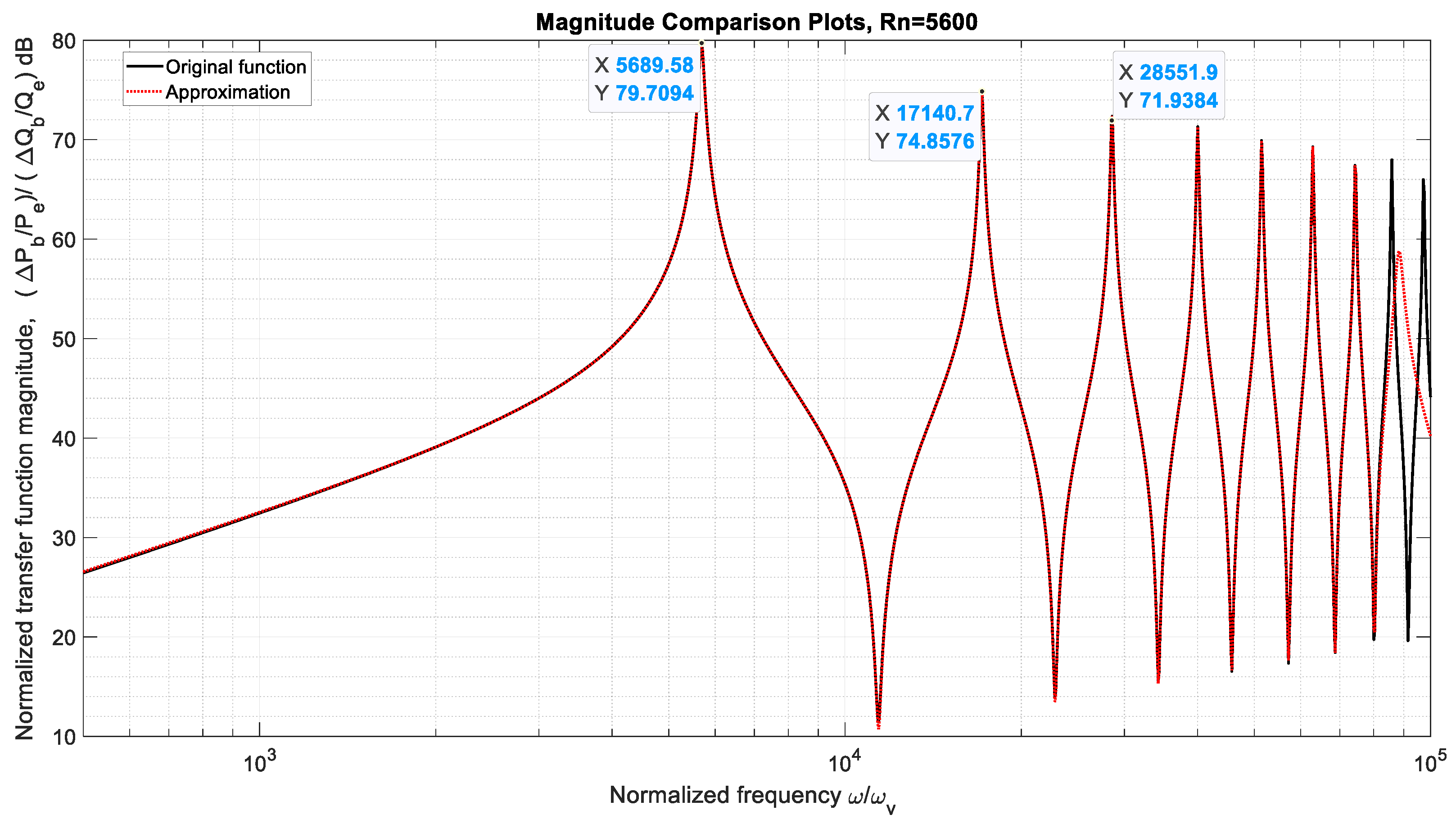
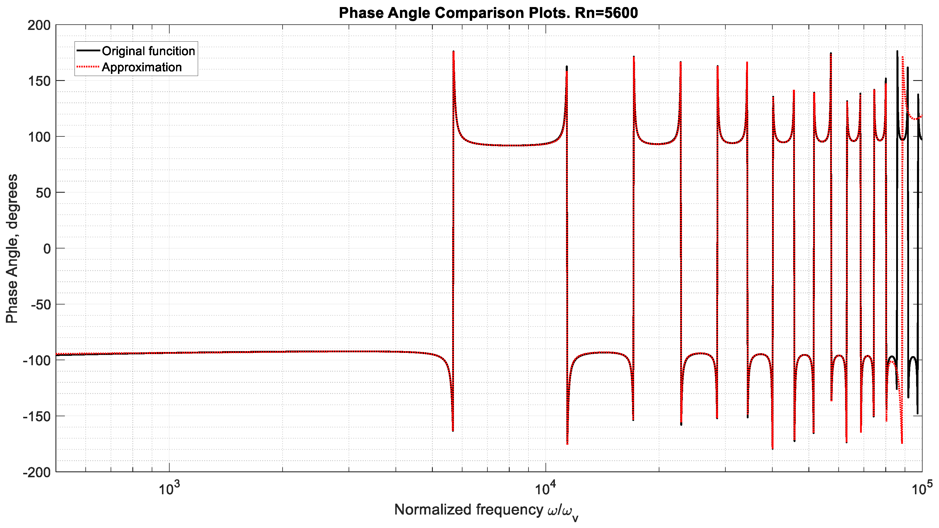
To generate the water hammer time domain solution for $\overline{\Delta P_b}\left(\overline{t}\right)$, the recommended first step is to obtain a frequency response plot of ${\left[{\displaystyle \frac{a_{12}\left(\overline{s}\right)}{a_{22}\left(\overline{s}\right)}}\right]}_{\overline{s}=j\overline{\omega }}$. The choice for the range of frequencies in the frequency response should consider the mode frequencies of the system and the input frequencies. Theoretically, a step change consists of frequencies from 0 to $\infty ;$ thus, for water hammer studies, the maximum frequency should be increased by trial and error until convergence representing the desired degree of no change is achieved. The second step will be to use an inverse frequency algorithm to obtain a finite order approximation for the frequency response over the specified range of frequencies. An example of the results using an inverse frequency algorithm is shown in Figure 2, Figure 3 and Figure 4 for a water line 37.23 m in length, with a 22.1 mm diameter, and with a pre-transient Reynolds number of 5600. These line dimensions and pre-transient flow conditions are associated with experimental data [17,31] used in the verification of the analytical solutions for turbulent flow [12].

Referring to the magnitude plots in Figure 2, it is of interest to note that the input specification to the inverse frequency algorithm was to obtain a match over the normalized frequency range from 10⁻¹¹ to 8 × 10⁴; the minimum value 10⁻¹¹ was chosen to calculate the DC gain near the correct value of 1 and the maximum value 8 × 10⁴ chosen to accurately include at least seven second order dominant modes. For purposes of resolution, the minimum normalized frequency shown on the graph is 500 even though 10⁻¹¹ was used in the algorithm. Also, note that the first three normalized resonant frequencies and peak values have been accurately identified with data tips. For example, at the normalized resonant frequency of 5689, the amplification of the sinusoidal pressure amplitude is ${10}^{{\displaystyle \frac{79.7}{20}}}=3.99.$ The order of the transfer function approximation was chosen to be 19 in order to obtain a good fit over the specified frequency range. It is very important to note the near perfect frequency response match (dotted lines) out to the designated upper frequency of 8 × 10⁴. An accurate match of the phase plots over the frequency range is confirmed in Figure 3.

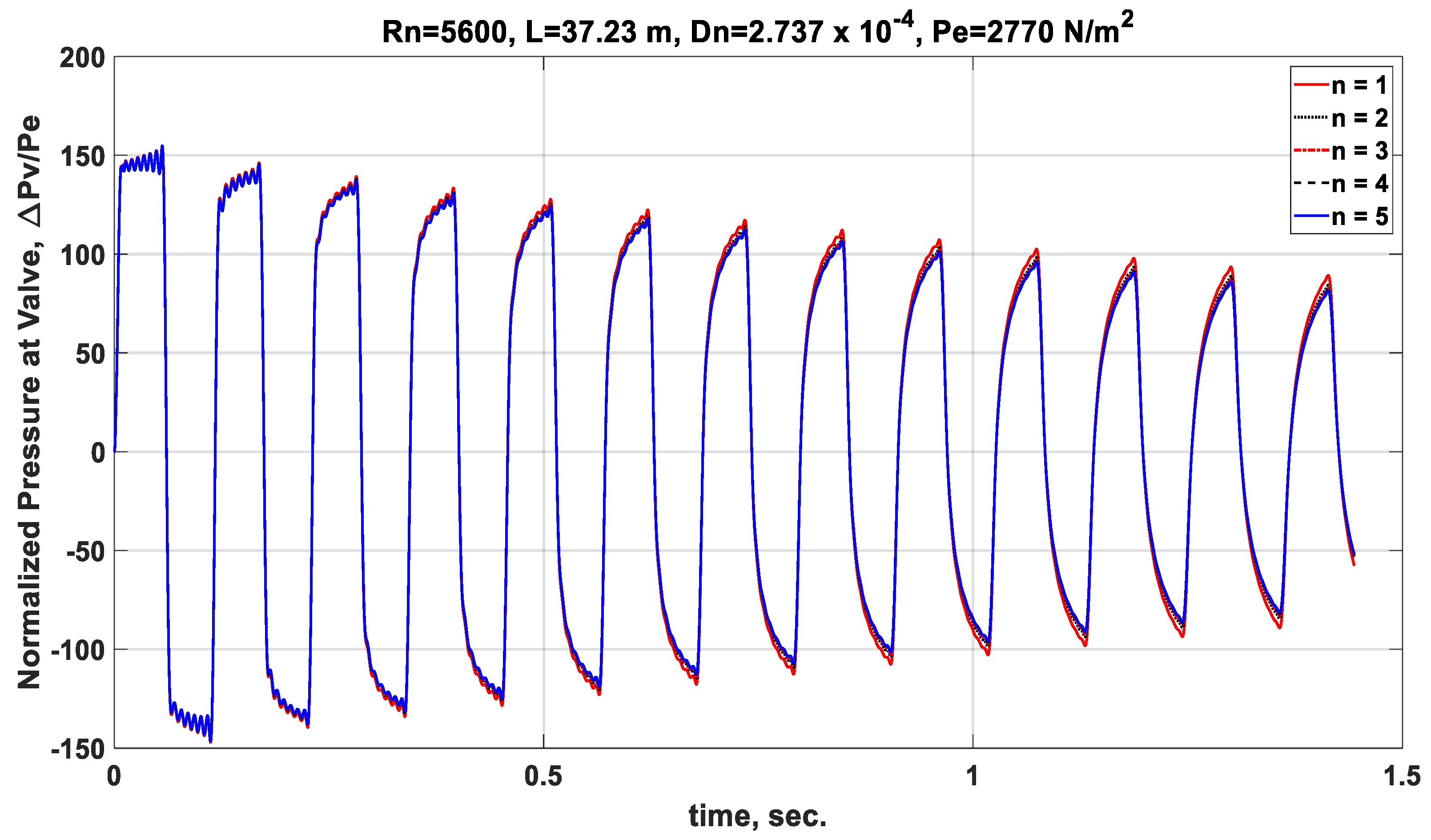
An important advantage of using an inverse frequency algorithm to generate a rational polynomial transfer function is that follow-up computer code can be used to generate time domain plots for specified inputs such as a step change associated with a water hammer. Typical results are shown in Figure 4 for 5 for different values of ‘n’. Recall that ‘n’ defines the distribution along the line of the additional losses due to turbulence. Validation with experimental results revealed that ‘n’ may need to be increased to an integer greater than 1 until decay rate convergence is confirmed [12]. A comparison of the plots reveals that ‘n’ = 1 would be sufficient for this low level of turbulence since increasing the value does not essentially change the decay rate of the oscillatory response. As shown in Figure 4, following valve closure, the initial pressure surge, due to water hammer, peaks at about 150$P_e$ = 4.155 × 10⁵ N/m².

3.2. Example 2—Lines with Pumps and Valves

Consider the schematic in Figure 5 of a line with a pump and a valve on the ends of the line. For this example, the passage area through the valve may be a function of time. For the pump, the output flow or pressure may be a function of time.

Assume the flow through the valve is defined by the orifice equation with variable area $A_v$ and coefficient $C.$ The nonlinear orifice equation that models forward or reverse flow is

$$P_b-P_d={\displaystyle \frac{Q_b\left|Q_b\right|}{C^2{A}_{ve}^2}}$$

(7)

Considering that the transfer function matrix in Equation (4) pertains to small perturbations relative to the pre-transient flow conditions, linearizing Equation (7) is possibly justified. Linearizing Equation (7) by taking the partial derivatives of the right side of Equation (7) about the pre-transient steady-flow conditions gives

$${∆P}_b-{∆P}_d={\displaystyle \frac{2Q_e}{C^2{A}_{ve}^2}}{∆Q}_b-{\displaystyle \frac{2Q_e^2}{C^2{A}_{ve}^3}}∆A_v$$

(8)

To maintain consistency with the line transfer function equations, the pressure and flow variables are normalized by the equation for pre-transient steady flow through the line, i.e.,

$$\overline{{∆P}_b}-\overline{{∆P}_d}=q\left(\overline{{\Delta Q}_b}-\overline{{\Delta A}_v}\right)$$

(9)

The dimensionless parameter q represents the ratio of the pre-transient linearized valve resistance to the line steady-flow resistance, i.e., $q={\displaystyle \frac{2Q_e^2}{C^2{A}_{ve}^2{P}_e}}$. Equations (4) and (9) contain 6-normalized perturbation variables, $\overline{{\Delta \mathrm{P}}_b},$ $\overline{{\Delta P}_a}$, $\overline{{\Delta Q}_a}$, $\overline{{\Delta Q}_b}$, $\overline{{\Delta P}_d}$, and $\overline{{\Delta A}_v}$, i.e.,

$$\overline{{\Delta P}_b}\left(\overline{s}\right)=a_{11}\overline{{\Delta P}_a}\left(\overline{s}\right)+a_{12}\overline{{\Delta Q}_a}\left(\overline{s}\right)$$

(10)

$$\overline{{\Delta Q}_b}\left(\overline{s}\right)=a_{21}\overline{{\Delta P}_a}\left(\overline{s}\right)+a_{22}\overline{{\Delta Q}_a}\left(\overline{s}\right)$$

(11)

$$\overline{{\Delta P}_b}\left(\overline{s}\right)-\overline{{\Delta P}_d}\left(\overline{s}\right)=q\left[\overline{{\Delta Q}_b}\left(\overline{s}\right)-\overline{{\Delta A}_v}\left(\overline{s}\right)\right]$$

(12)

Thus, to complete the solution, one or more of the variables must be designated as input(s) and/or additional equations added. Consider the examples in the following section.

3.2.1. Case 1—Constant Flow from Pump with Changing Valve Area

Suppose changes in the valve area, $\overline{{\Delta A}_v}\left(t\right),$ is designated to be an input. Assume the pump has a fixed displacement with a constant output flow, $\overline{{\Delta Q}_a}\left(t\right)=0$, and the value output pressure is constant, $\overline{{\Delta P}_b}\left(t\right)=0.$ If the output of interest is $\overline{{\Delta Q}_b}$, then Equations (10)–(12) simplify to give the desired transfer function equation, i.e.,

$$\overline{{\Delta Q}_b}\left(\overline{s}\right)=\left[{\displaystyle \frac{1}{1-\frac{a_{11}}{q{a}_{21}}}}\right]\overline{{\Delta A}_v}\left(\overline{s}\right)$$

(13)

Time domain plots of $\overline{{\Delta Q}_b}\left(\overline{t}\right)$ for different valve area changes $\overline{{\Delta A}_v}\left(\overline{t}\right)$ can be generated once the transfer function in Equation (13) is approximated by a ratio of finite order rational polynomials. The steps for achieving the finite order transfer function and then generating a time domain solution for $\overline{{\Delta Q}_b}\left(\overline{t}\right)$ are the same as the steps used in generating Figure 4. In this case, the input $\overline{{\Delta A}_v}\left(\overline{t}\right)$ can be any function of normalized time. It is important to note that the eigenvalues of the finite order transfer function reveal the resonant frequencies of the line; the input frequencies associated with changes in the valve area should be well below the eigenvalue frequencies to avoid potentially damaging pressure pulsations in the line associated with the fluid transients.

3.2.2. Case 2—Constant Valve Area with Changing Flow from a Variable Displacement Pump

This is a case where fluid transients may be desired and are likely to improve the performance of the system. Pumps are often used to force non-Newtonian fluids into downhole fissures in rock formations for oil and gas production. Pulsating flow rates from variable displacement pumps at resonant frequencies of the pressure transients in lines can enhance the performance of the system significantly. Theoretically, the resonant frequencies correspond to the resonant peaks on a frequency response. In practice, the resonant frequencies are determined by monitoring the pump output pressure, which will also peak at the resonant frequencies. The transfer function for perturbations in the downhole flow rate can be obtained from Equations (10)–(12). Assuming $\overline{{\Delta Q}_a}\left(t\right)$ is specified to be an oscillating input and ${\overline{∆P}}_d\left(t\right)=0$ and $\overline{{\Delta A}_v}\left(t\right)=0$, Equations (10)–(12) simplify to

$$\overline{{\Delta Q}_b}\left(\overline{s}\right)=\left[{\displaystyle \frac{a_{12}{a}_{21}-a_{11}{a}_{22}}{q{a}_{21}-a_{11}}}\right]\overline{{\Delta Q}_a}\left(\overline{s}\right)$$

(14)

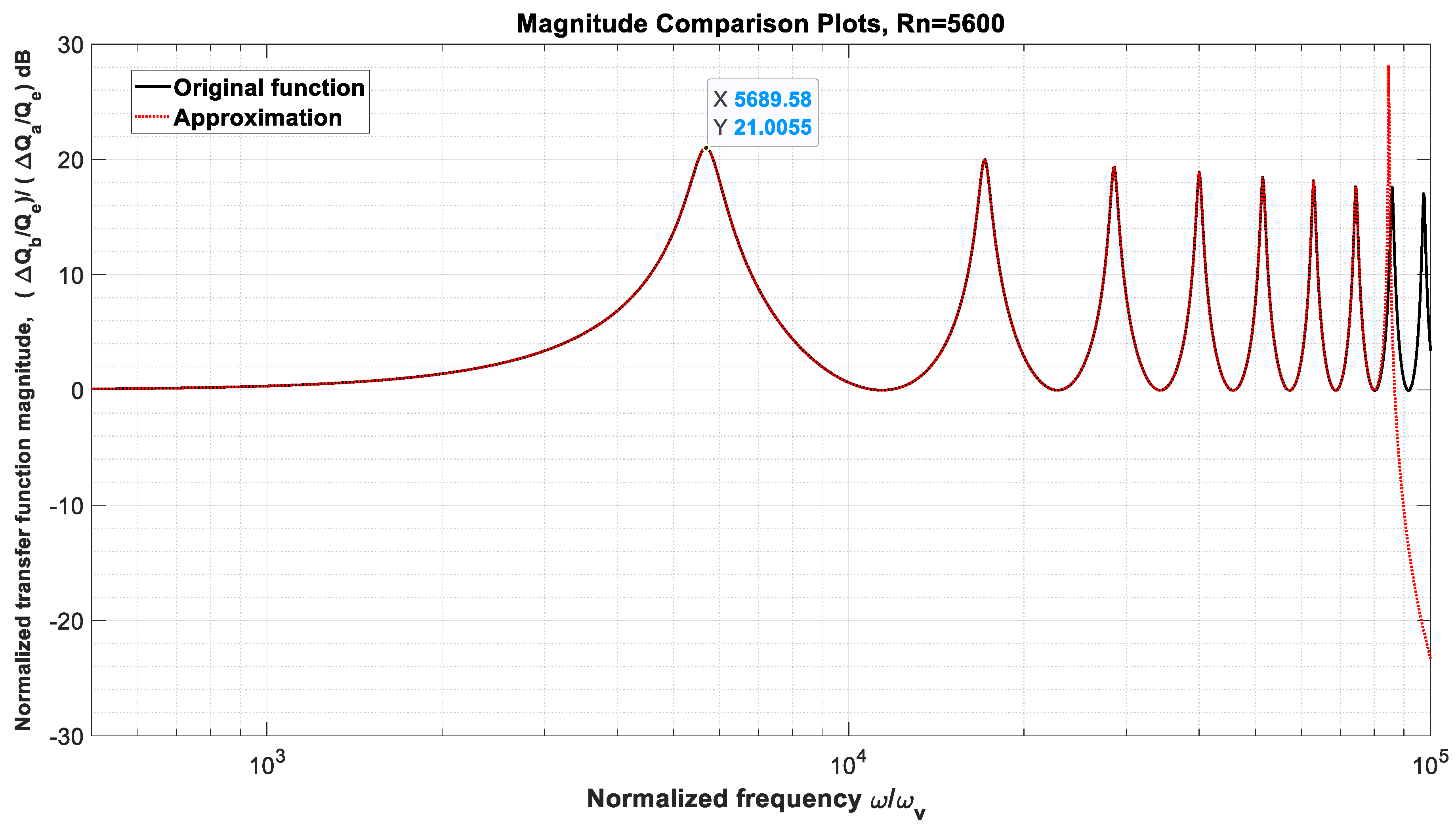
The frequency response of the transfer function in Equation (14) is shown in Figure 6.

As with previous transfer functions derived in this section, the transfer function in Equation (14) is infinite order. As shown in Figure 6, a frequency response of this transfer function with q = 10 reveals that the first mode resonant frequency occurs at a normalized frequency of 5689 with a dynamic gain of 21 dB. Thus, for a sinusoidal flow rate out of the pump at this resonant frequency superimposed on a mean flow, the amplitude of the sinusoidal output flow rate perturbations at the end of the line will be ${10}^{{\displaystyle \frac{21}{20}}}=11.22$ times larger than the input amplitude. The results and accuracy of the inverse frequency algorithm are also shown in Figure 6; having an approximation for the transfer function enables one to generate time domain plots of $\overline{{\Delta Q}_b}\left(\overline{t}\right)$ for any other pump output flow rate specifications such as pulses, etc.

3.3. Example 3—Rotary Actuator Controlled by a Variable Displacement Pump

A variable displacement pump is used to power and control the speed of a hydraulic motor (rotary actuator) [32]. A schematic of the system is shown in Figure 7.

The rotation speed, ${\dot{\theta }}_p,$ of the pump input shaft is assumed to be constant. The rotation direction and speed of the motor is determined by the direction and magnitude of the flow in the lines, which is determined by the pump displacement control lever. The significance of the fluid dynamics and flow losses in the lines are functions of the length and diameter of the lines and the frequencies of the input $\varnothing \left(t\right)$ and the load torque $T_L\left(t\right)$. The variables labeled on the schematic indicate the positive direction of the flows corresponding to counterclockwise rotation of the motor and clockwise torque representing the load on the motor shaft opposing the rotation of the motor. Most likely, it would be desirable for the input frequencies from the pump and/or load torque to be well below the resonant frequencies of the total system, which are defined by the fluid transients coupled with the load dynamics.

The following derivation formulates the transfer function for the total system, which provides the dominant eigenvalue resonant frequencies, which should be significantly lower than the frequencies of changes in the swash angle and/or load torque. The pump displacement $D_p$ is proportional to the swash plate angle $\varnothing$; thus, the flow from the pump in terms of the pump shaft angular velocity ${\dot{\theta }}_p$ is

$$Q_{ap}=D_p{\dot{\theta }}_p=C_p{\dot{\theta }}_p\varnothing$$

(15)

The flow through the motor is proportional to the motor displacement $D_m$, i.e.,

$$Q_{am}=D_m{\dot{\theta }}_m$$

(16)

The torque equation on the motor shaft is

$$J{\ddot{\theta }}_m+b_f{\dot{\theta }}_m+C_m{D}_m\left(P_{am}-P_{bm}\right)+T_L=0$$

(17)

where $J$ is the rotational inertia of the load, $b_f$ is a viscous damping coefficient, and $C_m$ is the motor torque coefficient.

Laplace transforming Equations (15)–(17) and then rewriting in small perturbation normalized format gives

$$\overline{∆Q_{ap}}(\overline{s})={\displaystyle \frac{C_p{\dot{\theta }}_p}{Q_e}}∆\varnothing (\overline{s})$$

(18)

$$\overline{∆Q_{am}}(\overline{s})={\displaystyle \frac{D_m{\nu }_e}{Q_e{r}_o^2}}\overline{s}∆{\theta }_m\left(\overline{s}\right)$$

(19)

$$\left[\left({\displaystyle \frac{J{\nu }_e^2}{P_e{r}_o^4}}\right){\overline{s}}^2+\left({\displaystyle \frac{{\nu }_e{b}_f}{P_e{r}_o^2}}\right)\overline{s}\right]∆{\theta }_m\left(\overline{s}\right)+C_m{D}_m\left[\overline{∆P_{am}}\left(\overline{s}\right)-\overline{∆P_{bm}}\left(\overline{s}\right)\right]+{\displaystyle \frac{1}{P_e}}\Delta T_L=0$$

(20)

Using Equation (4) for line ‘a’ and for line ‘b’ (see Figure 7), we obtain the normalized perturbation equations for the fluid transients in the lines, i.e.,

$$\left[\begin{array}{c}\overline{∆P_{am}}\left(\overline{s}\right)\\ \overline{∆Q_{am}}\left(\overline{s}\right)\end{array}\right]=\left[\begin{array}{cc}{a}_{11}\left(\overline{s}\right)& a_{12}\left(\overline{s}\right)\\ a_{21}\left(\overline{s}\right)& a_{22}\left(\overline{s}\right)\end{array}\right]\left[\begin{array}{c}\overline{\Delta P_{ap}}\left(\overline{s}\right)\\ \overline{\Delta Q_{ap}}\left(\overline{s}\right)\end{array}\right]$$

(21)

$$\left[\begin{array}{c}\overline{∆P_{bp}}\left(\overline{s}\right)\\ \overline{∆Q_{bp}}\left(\overline{s}\right)\end{array}\right]=\left[\begin{array}{cc}{a}_{11}\left(\overline{s}\right)& a_{12}\left(\overline{s}\right)\\ a_{21}\left(\overline{s}\right)& a_{22}\left(\overline{s}\right)\end{array}\right]\left[\begin{array}{c}\overline{\Delta P_{bm}}\left(\overline{s}\right)\\ \overline{\Delta Q_{bm}}\left(\overline{s}\right)\end{array}\right]$$

(22)

Assuming no leakage, we can write

$${∆Q}_{ap}={∆Q}_{bp}$$

(23)

$${∆Q}_{am}={∆Q}_{bm}$$

(24)

In Equations (18)–(24), there are two input variables, $∆\mathrm{\varnothing }$ and $∆T_L$, and there are nine unknowns, $\overline{∆Q_{ap}}\left(\overline{s}\right)$, $\overline{∆Q_{am}}\left(\overline{s}\right)$, $\overline{∆Q_{bp}}\left(\overline{s}\right)$, $\overline{∆Q_{bm}}\left(\overline{s}\right)$, $∆{\theta }_m\left(\overline{s}\right)$, $\overline{∆P_{am}}\left(\overline{s}\right)$, $\overline{∆P_{bm}}\left(\overline{s}\right)$, $\overline{∆P_{ap}}\left(\overline{s}\right)$, and $\overline{∆P_{bp}}\left(\overline{s}\right)$. Thus, it is possible to solve for the transfer functions for any of the unknown variables. For example, suppose that the output of interest is the perturbation in the motor speed $∆{\dot{\theta }}_m\left(t\right)$; this variable can be rewritten in normalized Laplace format, i.e.,

$$s∆{\theta }_m\left(s\right)={\displaystyle \frac{v_e}{r_o^2}}\overline{s}∆{\theta }_m\left(\overline{s}\right)$$

(25)

Eliminating all of the unknowns except $∆{\theta }_m\left(\overline{s}\right)$ from Equations (18)–(24) gives

$${\displaystyle \frac{v_e}{r_o^2}}\overline{s}∆{\theta }_m\left(\overline{s}\right)={\displaystyle \frac{\left[\frac{C_p{C}_m{D}_m{\dot{\theta }}_p}{Q_e}\left(1+a_{11}{a}_{22}-a_{12}{a}_{21}\right)\right]\Delta \varphi \left(\overline{s}\right)-\left[\frac{a_{21}}{P_e}\right]\Delta T_L\left(\overline{s}\right)}{\frac{J{\nu }_e{a}_{11}}{P_e{r}_o^2}\overline{s}+\frac{a_{21}{b}_f}{P_e}+\frac{C_m{D}_m^2}{Q_e}\left(a_{11}+a_{22}\right)}}$$

(26)

There are two transfer functions in Equation (26) for the inputs $∆\varnothing$ and $∆T_L$. Thus, the time history of the rotational speed of the motor, considering the fluid transients, can be obtained for any input specifications, deterministic or stochastic, once the transfer functions have been approximated by ratios of finite order polynomials, as demonstrated in the following example.

Assume an industrial excavator system with the following hydraulic system design specifications:

• Required peak motor torque: 5000 Nm
• Desired pre-transient motor speed: 10 RPM
• Pump peak pressure: 250 bar
• Pump speed: 1600 RPM
• Mass moment of inertia: $J=2\mathrm{k}\mathrm{g}{\mathrm{m}}^2$
• Viscous damping coefficient: $b_f=0{\displaystyle \frac{\mathrm{N}\mathrm{m}}{\mathrm{r}\mathrm{a}\mathrm{d}/\mathrm{s}}}$

Assume the fluid and line properties are

$${\rho }_e=850{\displaystyle \frac{\mathrm{k}\mathrm{g}}{{\mathrm{m}}^3}}{\nu }_e=0.0001{\displaystyle \frac{{\mathrm{m}}^2}{\mathrm{s}}}L=3\mathrm{m}{r}_o=0.0075\mathrm{m}a=1370\mathrm{m}/\mathrm{s}$$

A pre-transient motor flow of $Q_e=0.0002{\displaystyle \frac{{\mathrm{m}}^3}{\mathrm{s}}}$ corresponds to a Reynolds number of 170.

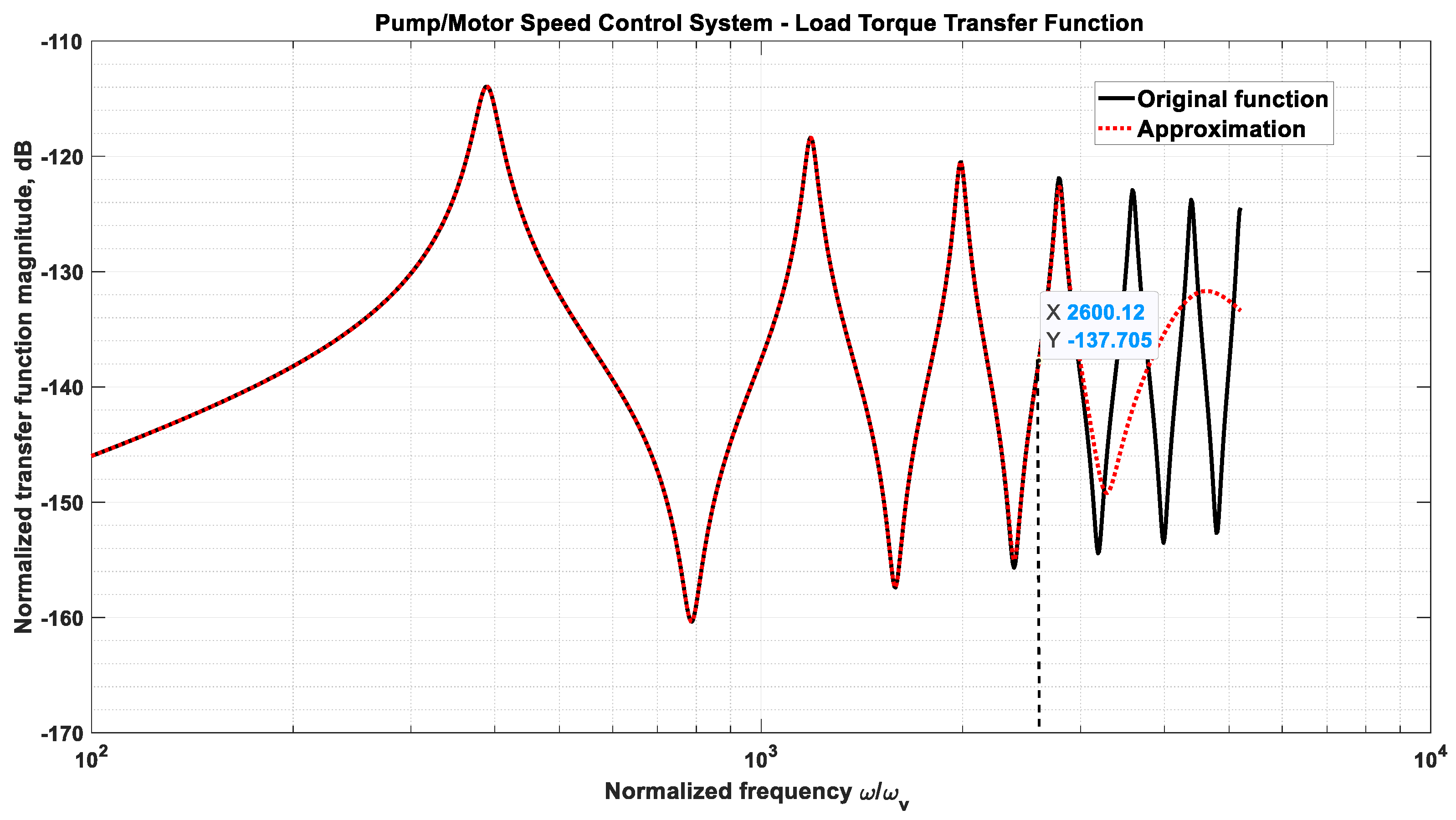
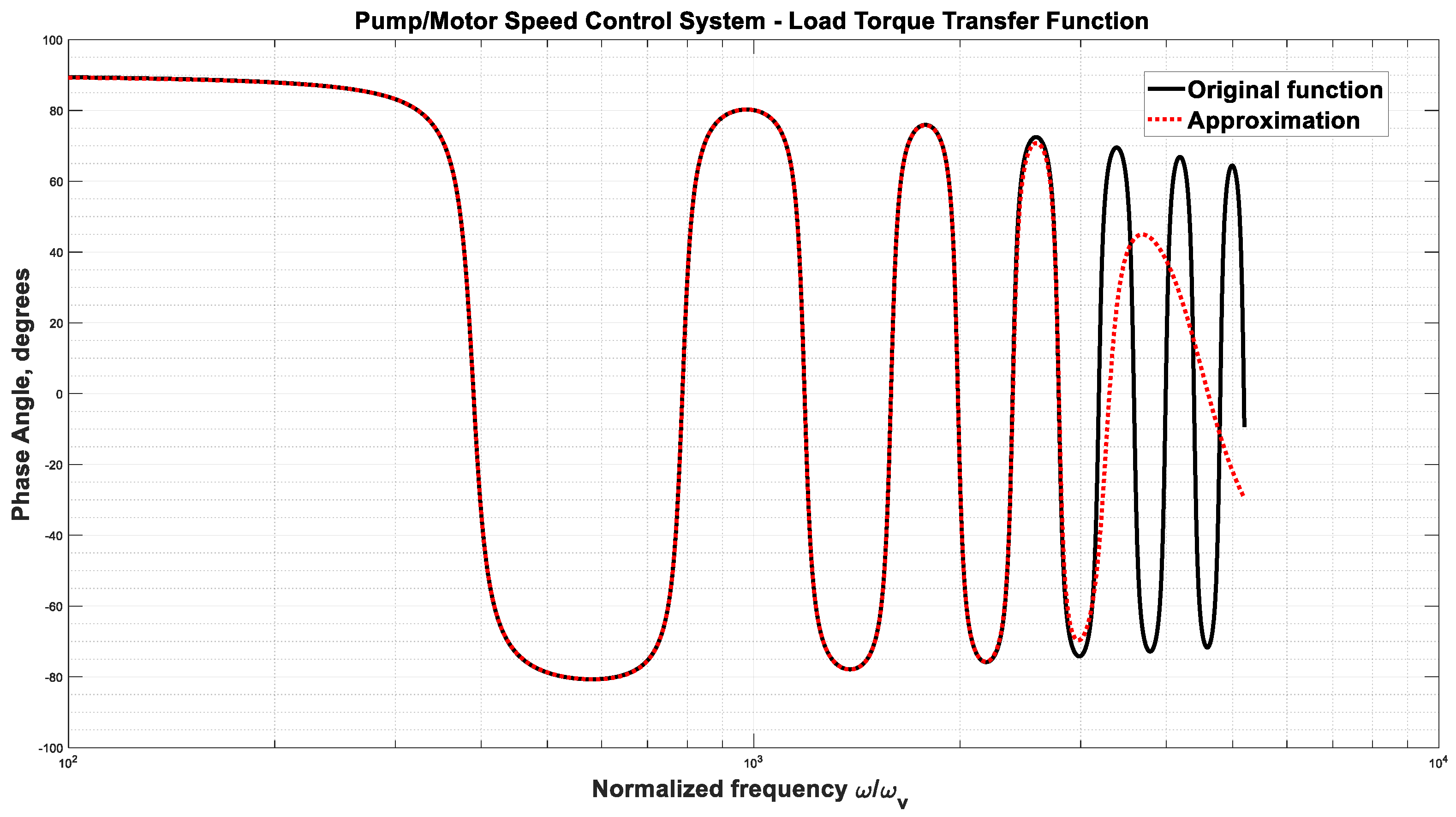
The frequency response for the load variation $∆T_L$ transfer function in Equation (26) and a 15th order transfer function approximation are shown in Figure 8 and Figure 9 for a matching normalized frequency range of 1 to 2600. Note the near perfect accuracy of the approximation, both magnitude and phase, over the specified frequency range and out to approximately 3000.

Examination of Figure 8 reveals the effects of the transmission line dynamics on the total system transfer function. That is, the transmission lines produce lightly damped changes to the motor RPM at the resonant frequencies of the total system. The choice of a 15th order approximation out to a maximum normalized frequency of 2600 was simply a trial-and-error test to gain insight into the system modes. Thus, knowing a range for potential input frequencies and the number of transfer function mode frequencies in that frequency range, it is possible that a much lower transfer function approximation would be sufficient for design and analysis studies of this system, as long as the DC gain of 0 is preserved.

Insight into potential reduced order approximations is gained by examining the normalized eigenvalues shown in

Table 1. Eigenvalues of the 15th order total system model.

Normalized Eigenvalues
$-28.9$
$-99.0$
$-265$
$-702$
$-1.43\times {10}^6$
$-14.7\pm j389$
$-25.1\pm j1190$
$-32.3\pm j1990$
$-39.8\pm j2790$
$-245\pm j4260$

for the 15th order system. Limiting the normalized frequency range of the approximation to 2600 for a 15th order transfer function approximation has resulted in five first order modes and five second order modes. It should be obvious why previous research studies attempting to use product series equations for the terms in the transfer function matrix have found it very difficult to know which 1st order modes to include [8].

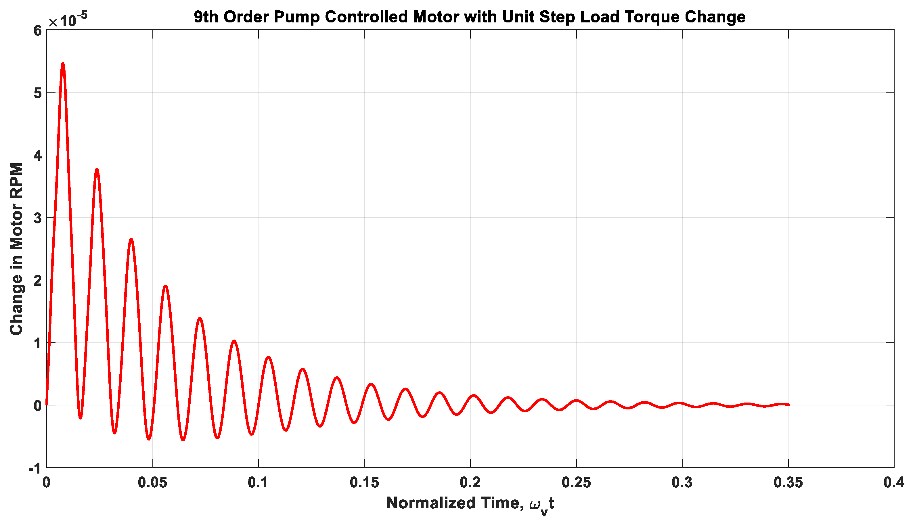
Insight into potentially reducing the order of the approximation can also be gained by generating a unit step response of the 15th order transfer function. Consider the step response shown in Figure 10.

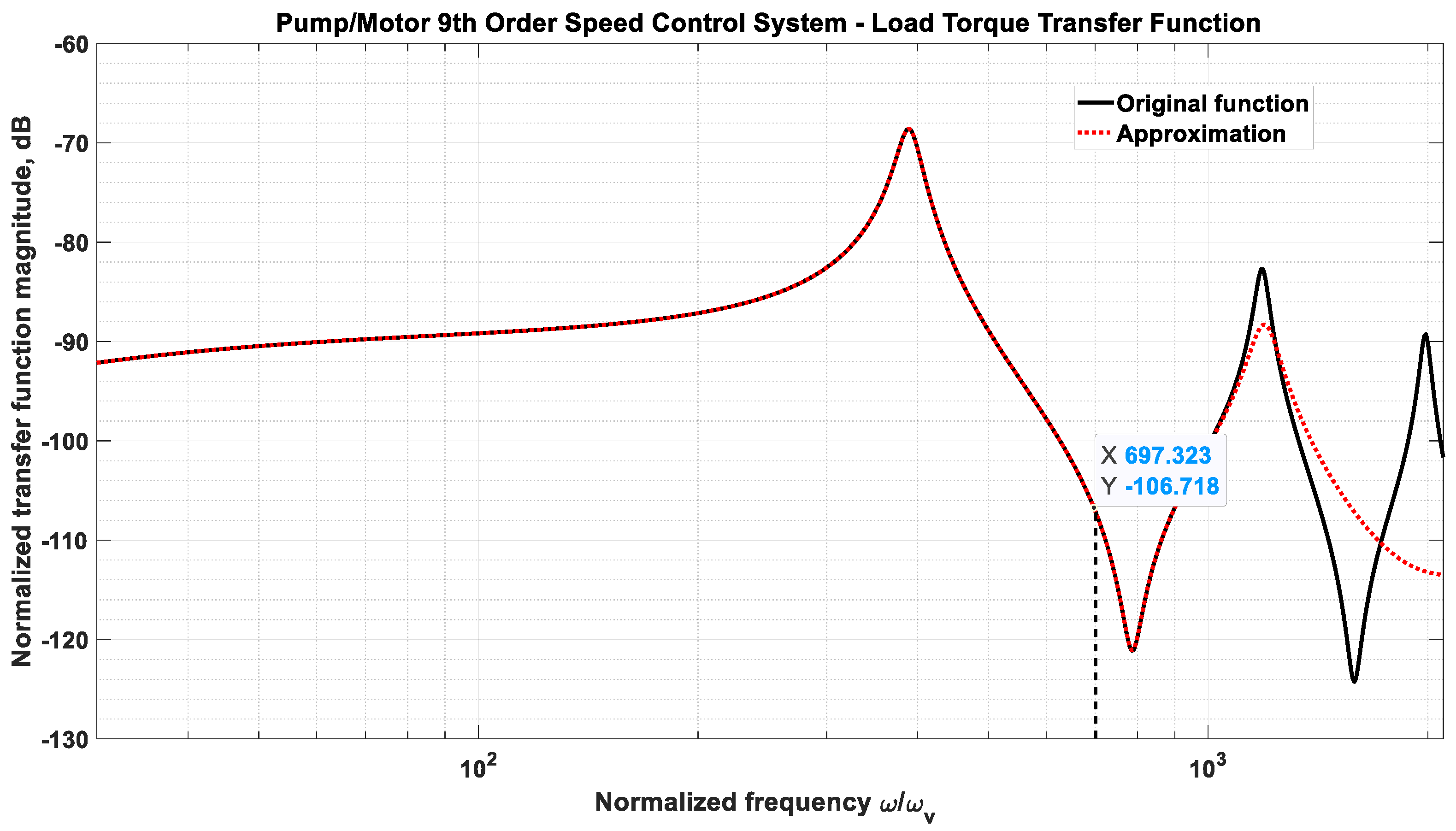
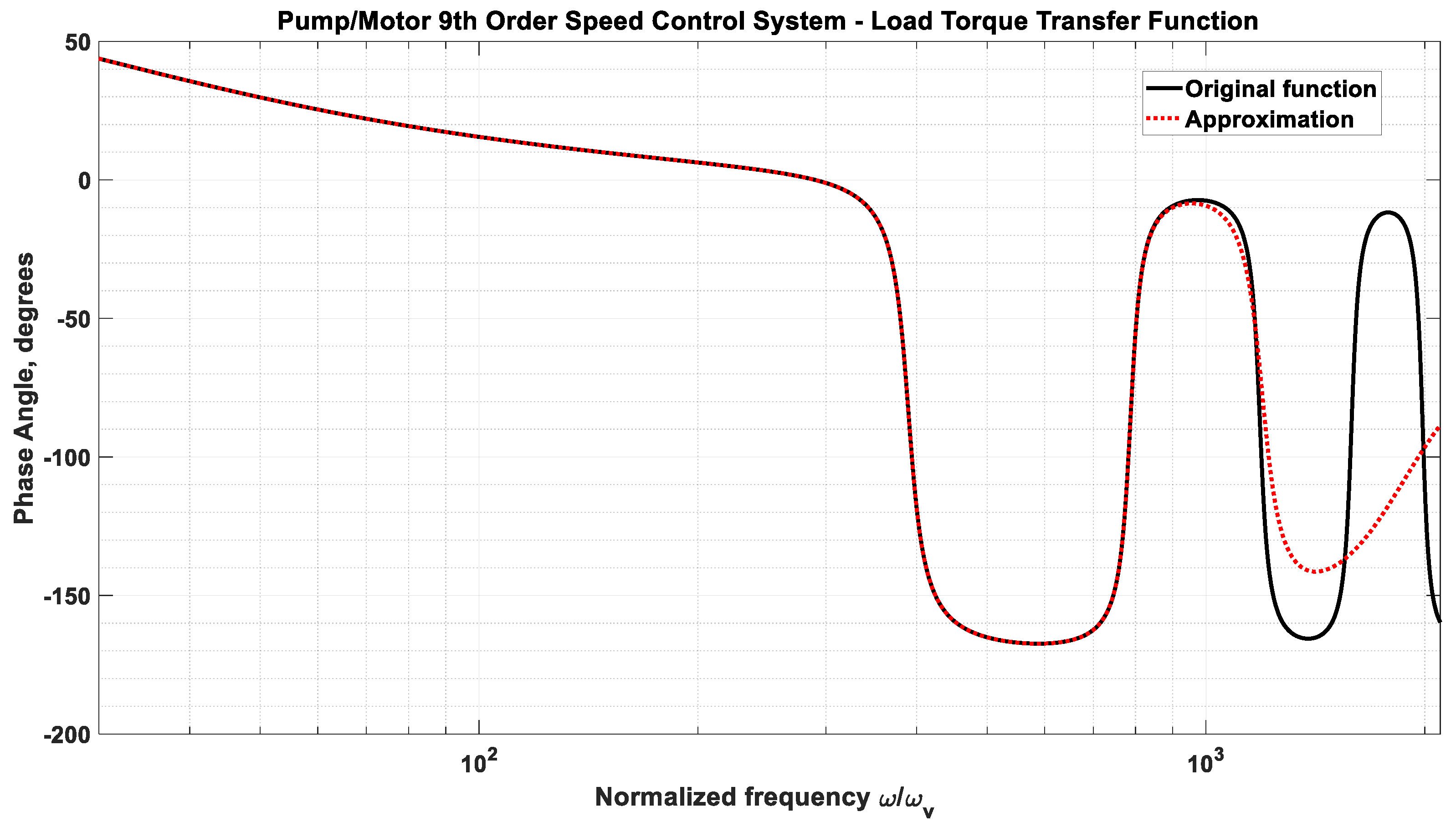
As shown in Figure 10, the normalized period of the oscillation (0.0395 − 0.02397) = 0.0155, which corresponds to a normalized frequency of 404. So, possibly by limiting the normalized frequency range to 700 instead of 2600 would it be possible to obtain a good fit with a lower order transfer function. The results for a ninth order transfer function approximation over a normalized frequency range of 1 to 700 are shown in Figure 11, Figure 12 and Figure 13.

The step response shown in Figure 13 for the 9th order transfer function approximation is essentially identical to the response in Figure 10 for a 15th approximation, and the DC gain of zero has been preserved.

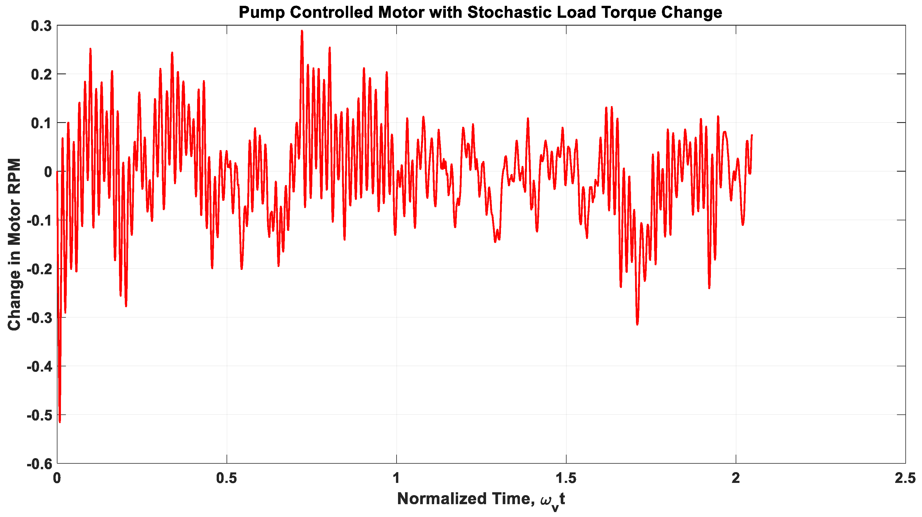
One final demonstration is to generate the normalize time response of the ninth order transfer function for a stochastic input defined by a power spectral density of ${\displaystyle \frac{1.27\times 10^7}{{\left(\omega /{\omega }_v\right)}^2}}$ for $100\le \omega /{\omega }_v\le 500$. The result shown in Figure 14 is typical of systems subject to noise and stochastic inputs associated with random load changes. Simulation results such as those shown in Figure 14 can be generated on most simulation platforms that can handle previously recorded data inputs from measurements.

4. Discussion

The results generated in this paper utilized the MATLAB R2024b platform. However, the results can be achieved with any software platform and computer languages that contain signal processing and system identification functions. Experience has revealed that the desired order of the transfer function approximation must take into account at least two times the number of second order modes observed in the necessary frequency range, plus additional unobserved first order modes that may exist. It is important to note that generation of an equivalent transfer function approximation will always be a trial and error process, starting with the frequency response of the infinite order system transfer function, which can be used to determine the frequency range for the approximation considering the input frequencies and an estimate of the order of the transfer function based on the observed modes. Experience has revealed that the desired order of the numerator should be set to one less than the order of the denominator, since unneeded coefficients will essentially end up being very small numbers close to zero.

An additional desired specification for the software platform is to be able to compute and plot time responses directly without having to reenter the transfer function approximation. For stochastic inputs, the platform must have a Fast Fourier transform function and statistical analysis functions. MATLAB mfiles used to generate the examples in this paper can be obtained by contacting the author directly.

5. Conclusions

The concept of ‘inverse frequency’ is to obtain an equivalent rational polynomial numerator and denominator transfer function approximation of a total system frequency response over a specified range of frequency response data for the total system. This approach is particularly applicable to the functions in Equation (4), which are obviously linear since the hyperbolic Bessel functions could have been expressed using infinite order product series [1,8]. In previous research, however, to obtain the transfer function approximations using the series formulations has proven to be very difficult, since it is never obvious which first order modes need to be included in order to not only maintain the low frequency accuracy associated with the DC gain but to also include critical first order modes at higher frequencies [8,18].

Accurate models for fluid transients in lines are defined by a set of simultaneous partial differential equations. As demonstrated in Appendix A, the analytical solution to these partial differential equations is obtained without having to specify specific details about components at the ends of the line. This is very desirable and provides significant versatilities to the analysis of the interaction of fluid transients with different end-of-line components that can be linearized for perturbations relative to pre-transient flow conditions. Examples demonstrating the method for model formulations and conversion from the frequency domain to the time domain have been presented. The analytical solution in Equation (4) is applicable to either laminar or turbulent pre-transient flow for Newtonian and a specific class of non-Newtonian fluids.

References

1. Goodson, R.E.; Leonard, R.G. A Survey of Modeling Techniques for Fluid Line Transients. ASME J. Basic Eng. 1971, 94, 474–482. [Google Scholar] [CrossRef]
2. Manhartsgruber, B. Transmission Line Models for Fluid Power Hoses Identified from Measurement Data. Fluid Power Syst. Technology. 2024, 88193, V001T01A026. [Google Scholar] [CrossRef]
3. Catania, G.; Sorrentino, S. Dynamical analysis of fluid lines coupled to mechanical systems taking into account fluid frequency-dependent damping and non-conventional constitutive models: Part 2—Coupling with mechanical systems. Signal Process. 2015, 50, 281–295. [Google Scholar] [CrossRef]
4. Bordbar, M. Analytical Solution of Quasi-Two-Dimensional Method for Unsteady Transient Pressurized Pipe Flows in the Time Domain. J. Hyd. Eng. 2025, 151, 04025035. [Google Scholar] [CrossRef]
5. Manhartsgruber, B. A Set of Benchmark Problems for Fluid Power System Simulation. Fluid Power Syst. Technol. 2022, 86335, V001T01A044. [Google Scholar] [CrossRef]
6. Kogler, H.; Scheidl, R.; Schmidt, B.H. Analysis of Wave Propagation Effects in Transmission Lines due to Digital Valve Switching. Fluid Power Syst. Technol. 2015, 57236, V001T01A057. [Google Scholar] [CrossRef]
7. Brunone, B.; Meniconi, S.; Capponi, C. The Damping of Pressure Peaks during Transients for Fault Detection in Pressurized Pipelines: An Expeditious and Manager-Oriented Diagnosis Procedure. J. Hydraul. Eng. 2023, 149, 02523002. [Google Scholar] [CrossRef]
8. Hullender, D.A.; Healey, A.J. Rational Polynomial Approximations for Fluid Transmission Line Models. In Fluid Transmission Line Dynamics, Proceedings of the Winter Annual Meeting, Washington, DC, USA, 15–20 November 1981; American Society of Mechanical Engineers: New York, NY, USA, 1981; pp. 33–55. [Google Scholar]
9. Urbanowicz, K.; Jing, H.; Bergant, A.; Stosiak, M.; Lubecki, M. Progress in Analytical Modeling of Water Hammer. J. Fluids Eng. 2023, 145, 081203. [Google Scholar] [CrossRef]
10. Braun, R.; Nordin, P.; Ericson, L.; Viktor, L.; Krus, P.; Pettersson, M. Hopsan: An Open-Source Tool for Rapid Modelling and Simulation of Fluid and Mechatronic Systems. Fluid Power Syst. Technol. 2020, 83754, V001T01A047. [Google Scholar] [CrossRef]
11. Bruhl, M. Analytical Solution for Laminar Water Hammer with Frequency-Dependent Friction. J. Fluids Eng. 2020, 144, 111302. [Google Scholar] [CrossRef]
12. Hullender, D. Alternative Approach to Modeling Transients in Smooth Pipe with Low Turbulent Flow. ASME J. Fluids Eng. 2016, 138, 121202. [Google Scholar] [CrossRef]
13. Hullender, D. Water Hammer Peak Pressures and Decay Rates of Transients in Smooth Lines with Turbulent Flow. ASME J. Fluids Eng. 2018, 140, 061204. [Google Scholar] [CrossRef]
14. Wongopotorn, P.; Hullender, D.A.; Woods, R.L. Rational Polynomial Transfer Function Approximations for Fluid Transients in Lines. Fluids Eng. Div. Summer Meet. 2003, 36967, 2797–2804. [Google Scholar] [CrossRef]
15. Urbanowicz, K.; Bergant, A.; Grzejda, R.; Stosizk, M. About Inverse Laplace Transform of a Dynamic Viscosity Function. Materials 2022, 15, 4364. [Google Scholar] [CrossRef] [PubMed]
16. Bergant, A.; Zlatko, R.; Urbanowicz, K. Analytical, Numerical 1D and 3D Water Hammer Investigations in a Simple Pipeline Apparatus. Stroj. Vestn.-J. Mech. Eng. 2025, 71, 149–156. [Google Scholar] [CrossRef]
17. Bergant, A.; Simpson, A.R.; Vitkovsk, J. Developments in Unsteady Pipe Flow Friction Modelling, ASCE. J. Hydraul. Res. 2001, 39, 249–257. [Google Scholar] [CrossRef]
18. Hullender, D.A.; Woods, R.L.; Hsu, C.H. Time Domain Simulation of fluid Transmission Lines Using Minimum Order State Variable Models. In N: Fluid Transmission Line Dynamics 1983, Proceedings of the Winter Annual Meeting, Boston, MA, USA, 13–18 November 1983; American Society of Mechanical Engineers: New York, NY, USA, 1983; pp. 51–78. [Google Scholar]
19. Regetz, J.D., Jr. An Experimental Determination of the Dynamic Response of a Long Hydraulic Line; National Aeronautics and Space Administration: Washington, DC, USA, 1960; Technical Note D-576.
20. Hullender, D. Analytical non-Newtonian Oldroyd-B transient model for pre-transient turbulent flow in smooth circular lines. J. Fluids Eng. 2019, 141, 021303. [Google Scholar] [CrossRef]
21. Bird, R.B.; Armstrong, R.C.; Hassager, O. Dynamics of Polymeric Liquids, 2nd ed.; Wiley: New York, NY, USA, 1987; Chapter 2; Volume 1. [Google Scholar]
22. Oldroyd, J.G. Non-Newtonian effects in steady motion of some idealized elastic-viscous liquids. Proc. R. Soc. 1958, A 245, 278–297. [Google Scholar]
23. Oldroyd, J.G. On the formulation of rheological equations of state. Proc. R. Soc. 1950, A 200, 523–541. [Google Scholar]
24. McGinty, S.; McKee, S.; McDermott, R. Analytic Solutions of Newtonian and Non-Newtonian Pipe Flows Subject to a General Time-Dependent Pressure Gradient. J. Non-Newton. Fluid Mech 2009, 162, 54–77. [Google Scholar] [CrossRef]
25. Garcia, F.J.G.; Alvarino, P.F. On the analytic explanation of experiments where turbulence vanishes in pipe flow. J. Fluid Mech. 2022, 951, A4. [Google Scholar] [CrossRef]
26. Urbanowicz, K.; Di Nucci, C.; Sharma, B.K.; Ashok, K.; Kawiak, M.; Krajewski, S. Revisiting Yamaguchi-Ichikawa water hammer model. Chin. J. Phys. 2025, 94, 487–503. [Google Scholar] [CrossRef]
27. Guse, F.; Pasquini, E.; Schmitz, K. Consideration of Air Bubble Dynamics in 1D Hydraulic Pipeline Simulation—Source Term Development and Verification Utilizing Transmission Line Theory. Fluid Power Syst. Technol. 2021, 85239, V001T01A002. [Google Scholar] [CrossRef]
28. Vıtkovsky, J.P.; Lee, P.J.; Zecchin, A.C.; Simpson, A.R.; Lambert, M.F. Head-and Flow-Based Formulations for Frequency Domain Analysis of Fluid Transients in Arbitrary Pipe Networks. ASCE J. Hydraul. Eng. 2011, 137, 556–568. [Google Scholar] [CrossRef]
29. Danes, L. The influence of line and fluid parameters on pressure ripple in hydraulic transmissions. SN Appl. Sci. 2020, 2, 1281. [Google Scholar] [CrossRef]
30. Bayle, A.; Rein, F.; Plouraboue, F. Frequency varying rheology-based fluid-structure-interactions wave in liquid-filled visco-elastic pipes. J. Sound Vib. 2023, 562, 117824. [Google Scholar] [CrossRef]
31. Adamkowski, A.; Lewandowski, M. Experimental Examination of Unsteady Friction Models for Transient Pipe Flow Simulation. ASME J. Fluids Eng. 2006, 128, 1351–1363. [Google Scholar] [CrossRef]
32. Blackburn, J.F.; Reethof, G.; Shearer, J.L. Fluid Power Control; The M.I.T. Press: Cambridge, MA, USA, 1960; Lib. of Congress Catalog No. 59-6759; pp. 499–508. [Google Scholar]
Figure 1. Schematic of a fluid transmission line with the input and output variables.
Actuators 14 00489 g001
Figure 2. Magnitude comparison of the frequency response of the inverse frequency linear transfer function approximation with the exact frequency response of the water hammer transfer function in Equation (6) for turbulent flow conditions.
Actuators 14 00489 g002
Figure 3. Phase angle comparison of the inverse frequency response approximation with the exact frequency response of the water hammer transfer function in Equation (6).
Actuators 14 00489 g003
Figure 4. Normalized pressure upstream of the value following valve closure demonstrating the pressure surge and wave frequency in the line and demonstrating the insensitivity to the number ‘n’ for this relatively low level of turbulence.
Actuators 14 00489 g004
Figure 5. Schematic of a line with a pump and valve.
Actuators 14 00489 g005
Figure 6. Frequency response of the transfer function in Equation (20) for q = 10.
Actuators 14 00489 g006
Figure 7. Schematic of a rotary actuator speed control system.
Actuators 14 00489 g007
Figure 8. Normalized frequency response magnitude of the T L transfer function in Equation (26) compared to a 15th order rational polynomial approximation obtained using an inverse frequency algorithm.
Actuators 14 00489 g008
Figure 9. Normalized frequency response phase angle of the T L transfer function in Equation (26) compared to a 15th order rational polynomial approximation obtained using an inverse frequency algorithm.
Actuators 14 00489 g009
Figure 10. Unit step response of the 15th order transfer function approximation.
Actuators 14 00489 g010
Figure 11. Normalized frequency response magnitude of the T L transfer function in Equation (26) compared to a ninth order rational polynomial approximation obtained using an inverse frequency algorithm out to a normalized frequency of 700.
Actuators 14 00489 g011
Figure 12. Normalized frequency response phase angle of the T L transfer function in Equation (26) compared to a ninth order rational polynomial approximation obtained used an inverse frequency algorithm out to a normalized frequency of 700.
Actuators 14 00489 g012
Figure 13. Unit step response of the ninth order transfer function approximation.
Actuators 14 00489 g013
Figure 14. Normalized time response of the ninth order transfer function for a stochastic input defined by a power spectral density.
Actuators 14 00489 g014