FPI-Based Adaptive Control with Simultaneous Noise Filtering and Low Frequency Delay

Abstract

In the field of life sciences, delay effects are often modeled with two compartments that do not model any particular organ. In this paper the use of this double counterpart model is investigated in Fixed-Point Iteration-based (FPI) Control, which was introduced in 2009 as an adaptive extension to the Computed Torque Control method. This controller is particularly sensitive to delays and measurement noise due to its iterative nature. It was recognized that, besides modeling the delay effect, this signal tackling also provided the controller with some noise filtering ability; the formerly accumulated effects of noise filtering and formally delayed sampling were avoided. This smeared delay has a noticeable effect even slightly later in time, making the adaptive method based on it more robust. This assumption was investigated both on a simulation and experimental basis.

1. Introduction

In most robot applications the manipulator is tasked to follow some designated path as precisely as possible. Therefore, trajectory tracking is one of the most important and fundamental problems in field of robotics that is posing significant challenges due to the complicated, highly nonlinear and time-varying behavior of robotic manipulators. This fundamental problem has inspired numerous solutions over the years. Among these, Computed Torque Control (CTC) is a widely used and well established solution that was developed at the end of the 20th century [1]. This control method utilizes the dynamic model of the controlled system in a feed forward configuration with some linear error compensation rule, which is most commonly a PID (Proportional–Integral–Derivative) controller. Therefore, the effectiveness of the CTC method is limited by the accuracy of the system model and the precision of feedback signal measurements. In practice, position and velocity transducers are effected by quantization noise, and it also quickly became apparent that it presents significant challenges to develop precise enough robot models for control purposes [2].

However, given its simple structure and computational efficiency in comparison with certain adaptive and robust control solutions, CTC remained a prevalent approach within the field of robotics throughout the years, e.g., [3,4,5]. To address some of the design challenges, many researchers suggested adaptive or robust variations. For example, in the early years, a globally convergent Adaptive CTC method was suggested with a simple least square estimator in order to fine-tune the dynamic model parameters of the controlled manipulator [6]. In [7] a CTC was designed with a nonlinear PD (Proportional–Derivative) controller and an Extended State Observer to estimate external disturbances and modeling errors due to friction and temperature variations. It was shown that the nonlinear PD gains significantly improve the responsiveness of the controller, that way better tracking properties could be achieved for higher speed motion in case of a 6-DoF (Degree of Freedom) parallel manipulator. However, nonlinear PID controllers have a greater number of parameters that require careful tuning, thereby influencing the controller’s behavior in various unexpected manners. Hence, the use of soft computing methods, e.g., Particle Swarm Optimization [8,9], has been successfully investigated by many authors for tuning purposes. In order to ensure desired transient trajectory tracking behavior of a rehabilitation exoskeleton, a novel CTC design was introduced in [10] with a Prescribed Performance Controller, which is a widely used technique in adaptive control [11,12]. In order to address the issue of modeling imprecisions, the utilization of a neural network, such as a radial basis function neural network, was considered in the literature [13,14]. These methods are capable of compensating for complex nonlinearities and dynamic uncertainties. However, their practical implementation can be constrained by the high computational cost associated with online learning, which may not be feasible in real-time applications [15].

A robust iterative variation of the CTC method was developed in 2009 [16] for controlling second-order systems with uncertain dynamics, such as robots or CNC machines. The proposed control strategy does not rely on refining the imprecise dynamic model and it places the deterministic decrease in the trajectory tracking error in the center of attention. It adaptively deforms the desired acceleration command—derived from the kinematic prescription of the CTC controller—in order to ensure accurate trajectory tracking despite model uncertainties. The adaptive deformation is executed in an iterative manner, with a single update executed in each control cycle with low computation cost. As a result, the method is referred to as Robust Fixed-Point Transformation (RFPT)-based adaptive control. The concept of “adaptive control” has a long development history from the early nineties to present day. The “Parameter Adaptive” solutions (early prototype is [17]) used an analytically correct model form with imprecisely known parameters and learned the exact parameters of this model. The “Signal Adaptive” solutions (early example is, e.g., [18]) applied strong signals in order to make the behavior of the controlled system identical to that of a “Reference Model”. Recently, good results were achieved by manipulating the originally available dynamic model by transforming it into a Linear Parameter Varying form (e.g., [19]). Also, even model-free approaches can be found with Machine Learning (e.g., [20]). The RFPT-based controller corresponds to an approximate model-based controller that does not wish to “learn” the precise dynamic model. Instead of that, based on recent observations it applies temporal corrections that do not have a persistent nature. Consequently it cannot achieve asymptotic convergence. The cost of this deficiency is the way of easy realization. The convergence of the iteration applied in the RFPT method and hence the local stability of the control law can be analyzed using Banach’s fixed-point theorem [21], which states the following:

Let $(\mathcal{B},d)$ be a non-empty complete metric space, and let $\mathrm{\Phi }:\mathcal{B}\to \mathcal{B}$ be a contractive self mapping, i.e., there exists a constant $0<\gamma <1$ such that $d\left(\mathrm{\Phi }\right(x),\mathrm{\Phi }(y\left)\right)\le \gamma d(x,y)\mathrm{for}\mathrm{all}x,y\in \mathcal{B}$. Then, for any initial guess $x_0\in \mathcal{B}$, the sequence generated by Φ in the form of $\left\{x_0,x_1=\mathrm{\Phi }\left(x_0\right),x_2=\mathrm{\Phi }\left(x_1\right),...,x_n=\mathrm{\Phi }\left(x_{n-1}\right)\right\}$ converges to a unique $x^{*}\in \mathcal{B}$ such that $\mathrm{\Phi }\left(x^{*}\right)=x^{*}$.

This theorem provides the fundamentals for analyzing the convergence behavior of the proposed iterative control rule, ensuring that by the proper tuning of only a few parameters, the control signal converges reliably to a stable solution. The optimal tuning of the control parameters were investigated in [22]. For the actual implementation of the adaptive deformation a few variations exists. For example, the original idea was extended for MIMO (Multiple-Input and Multiple-Output) systems in [23,24]. A continuous time RFPT method was investigated in [25]. The noise sensitivity was addressed in [26] with a Luenberg observer-inspired solution. Additionally, a geometric formulation was proposed in [27], where the control signals were transformed into a higher-dimensional vector space, enabling abstract rotations that simplified the tuning process. A novel FPI control design was introduced in [28] with a Steffensen accelerator in order to improve the convergence rate and thereby the tracking precision of the controller. This solution was later extended to an Adaptive Sliding Mode Control design as well [29,30].

The application of FPI control was suggested across various scientific domains, ranging from controlling classical mechanical systems [31] to life sciences, such as automated anesthesiology [32,33] or blood glucose level regulation [34]. However, most of the existing research has been limited to simulation-based analysis. This limitation has motivated the authors to pursue further investigation of FPI control through experimental implementation, which revealed several practical challenges. Notably, in the case of second-order systems (i.e., industrial robots), the controller requires feedback not only of the first-order derivatives of the generalized coordinates (i.e., velocities), but also of their second-order derivatives (i.e., accelerations), which introduces sensitivity to measurement noise and estimation errors.

In our previous investigations the issues of noise filtering and delay were considered as formally separated issues, i.e., certain noise filtering techniques were applied for the signals, and the filtered signals were sampled with some exact delay. In this approach the inevitable delaying effect of the noise filtering technique was not taken into account, and it had an accumulated effect with that of the formally delayed sampling. In the present approach a delay modeling technique was borrowed from life sciences that corresponded to the application of a complementary, “anatomically not interpreted compartment”, in the state variable of which the effects of the “harsh”, non-continuous input appeared in a smoothed, smeared manner. Recognizing that besides modeling the delay effect this signal tackling also provided the controller with some noise filtering ability, the formerly accumulated effects of noise filtering and formally delayed sampling were avoided. A complementary benefit was that while the formally applied delay time must be very precisely specified in the calculations, this smeared effect was noticeable even slightly later in time, making the adaptive method based on it more robust.

The main challenge of the investigated problem consists in the fact that the above listed results related to the FPI-based adaptive solutions were made on the theoretical basis of Banach’s simple and efficient fixed-point theorem and were illustrated via simulations. These simulations had certain tacit assumptions that lead to a simplified model of the operation of the controlled system that cannot precisely cover the reality. While the issue of measurement noise was placed into the center of the considerations, subtle excerpts such as the properties of the operating system of the implementation, the cooperation of the signal measuring system with the control program, and the features of a possible embedded realization were not precisely simulated. This made the experimental investigations inevitable, which soon revealed differences between the simulation and the measurement results. The simple assumption of a fixed cycle time of the digital controller certainly is not realistic for several operating systems that can produce a control signal during longer or shorter times, depending on its other actual tasks and the computational need of the problem. Furthermore, the signal measuring system is not in harmony with the cycles of the controller. Normally it produces signals that are processed via interrupts. Since the method is based on the observation of the control signal and the observed response to it in the near past, timing discrepancies may have critical effects. The measurement results presented in this paper that the suggested low frequency noise filtering combined with the use of its inherent, inevitable delay, and a simple delay-smearing technology realized by common and cheap hardware and software tools are the first very successful experimental proofs of the real applicability of the adaptive method in a realistic problem. It reveals that the subtle details neglected in the simulations do not play a significant role in the system’s operation.

This proof widely extends the expected circle of the practical application of the FPI-based adaptive controller. For instance, the problem of fixed time stabilization of linear control systems solved in [35] may be extended to the stabilization of nonlinear ones by replacing the complicated Lyapunov function-based proofs with that based on the simple Banach’s theorem. Also, controlling the behavior of connected robots or other nonlinear systems governed by sophisticated, beyond nearest neighbor rules considered in [36] can be really tackled by this simpler approach. Formerly, simulation results were presented by the application of decentralized adaptive control of very imprecisely modeled coupled dynamic systems in [37], or that in the topologically less complex, “linear arrangement” of platoons considered in [38] arrived to the phase of physical realization. This adaptive method can be combined with topologically formulated, more complex and sophisticated task definitions.

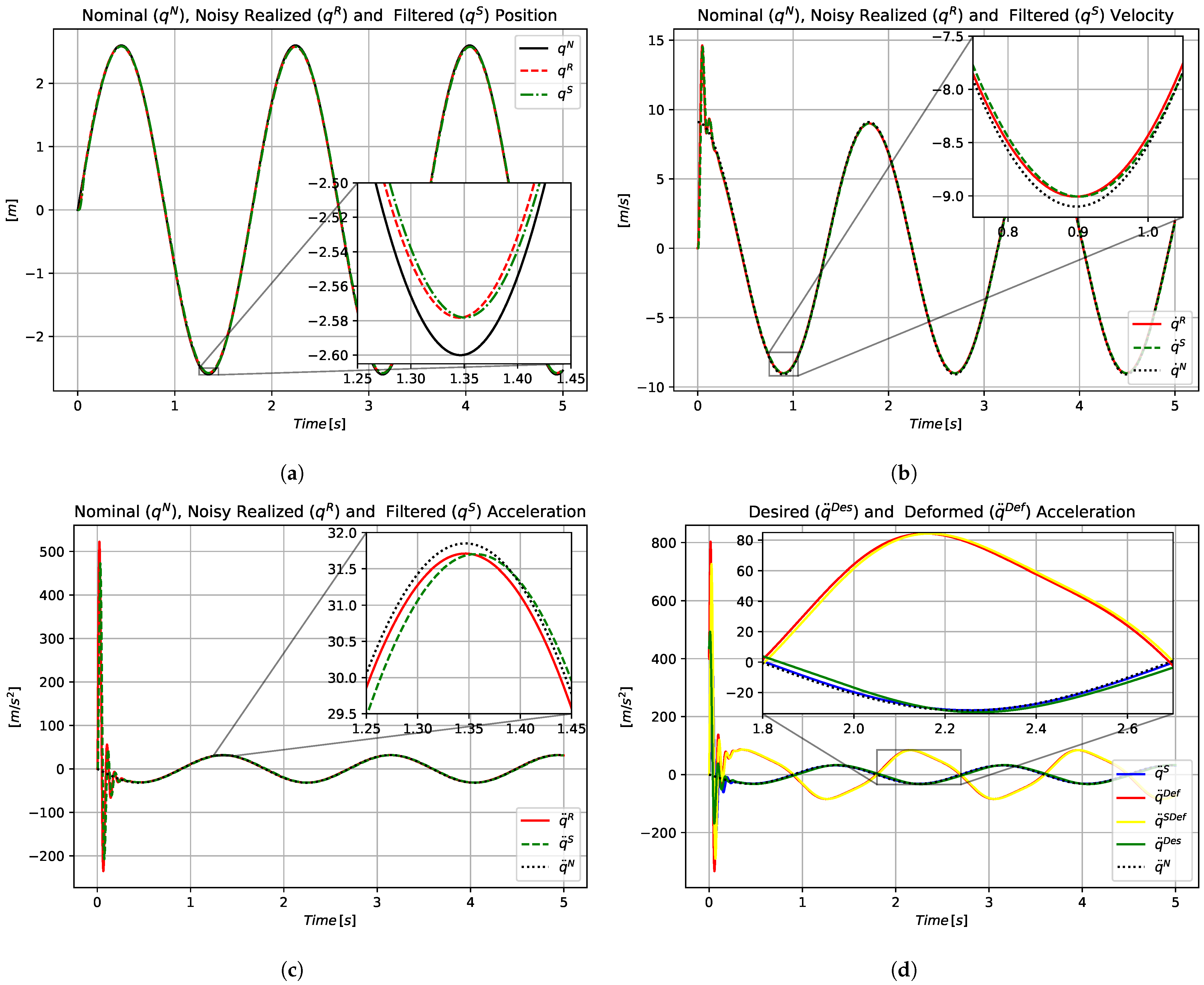
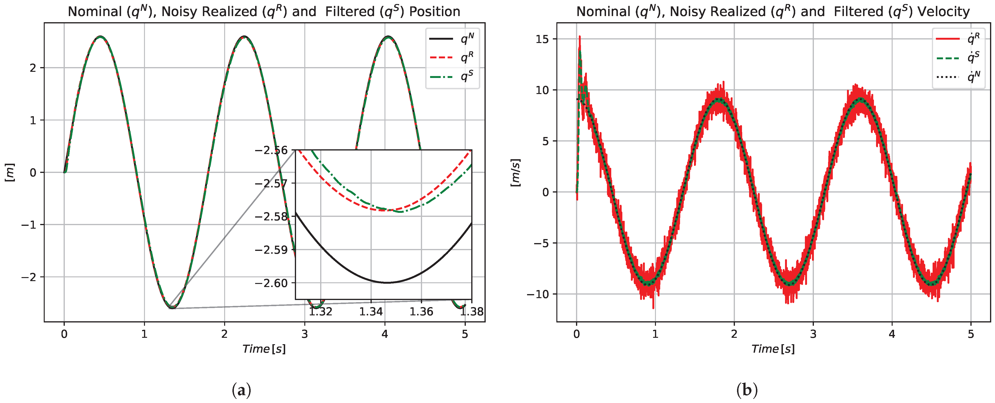
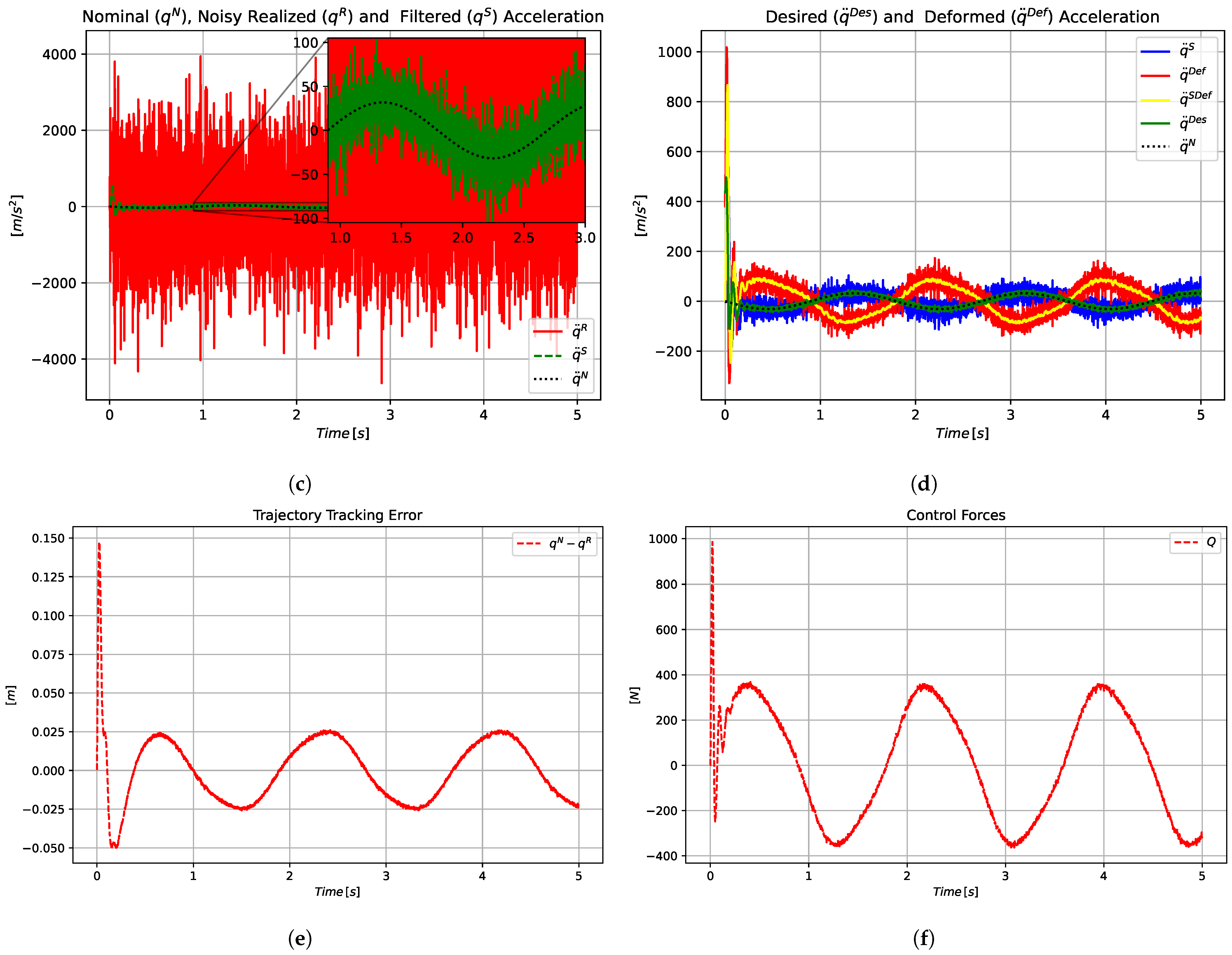
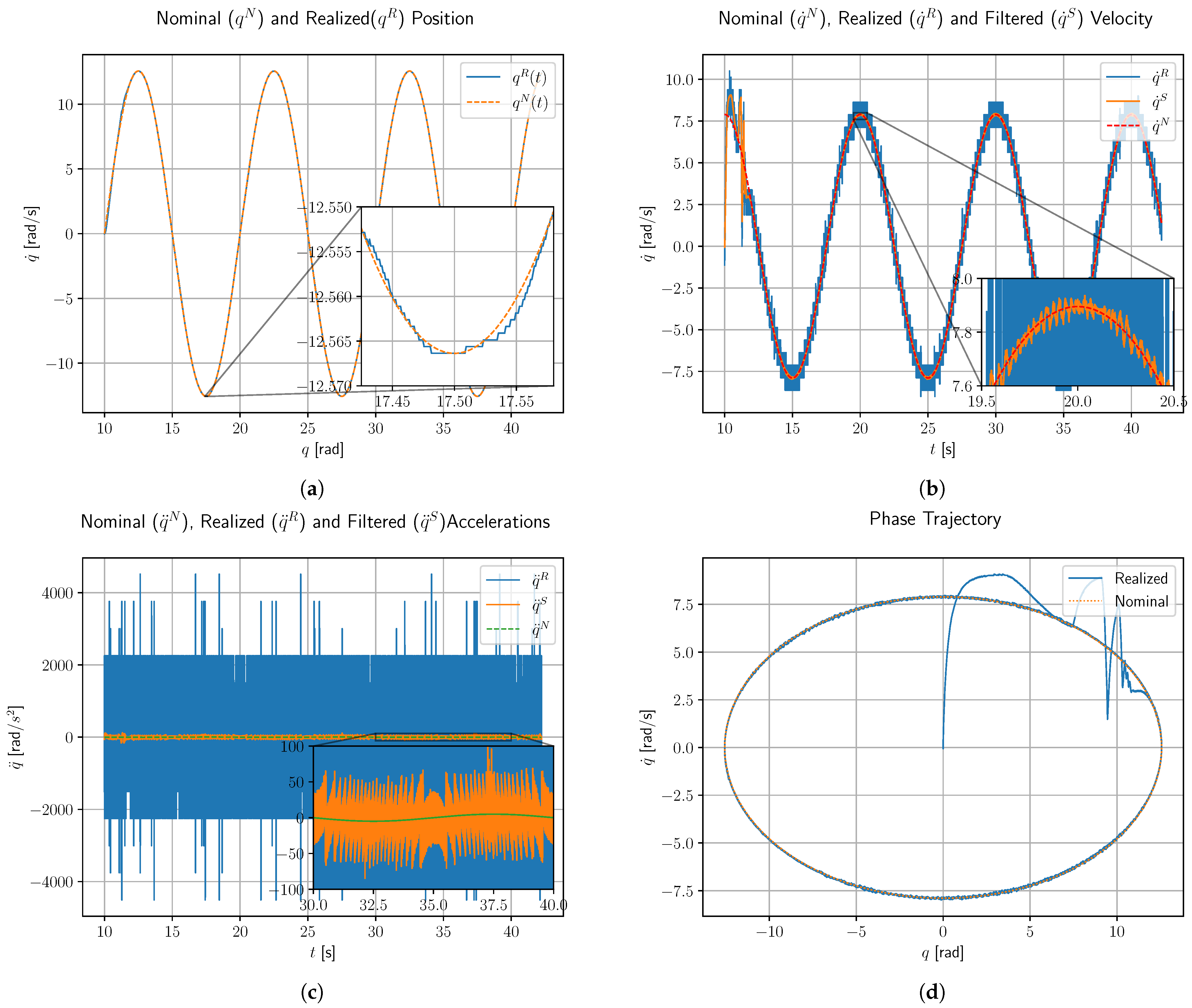
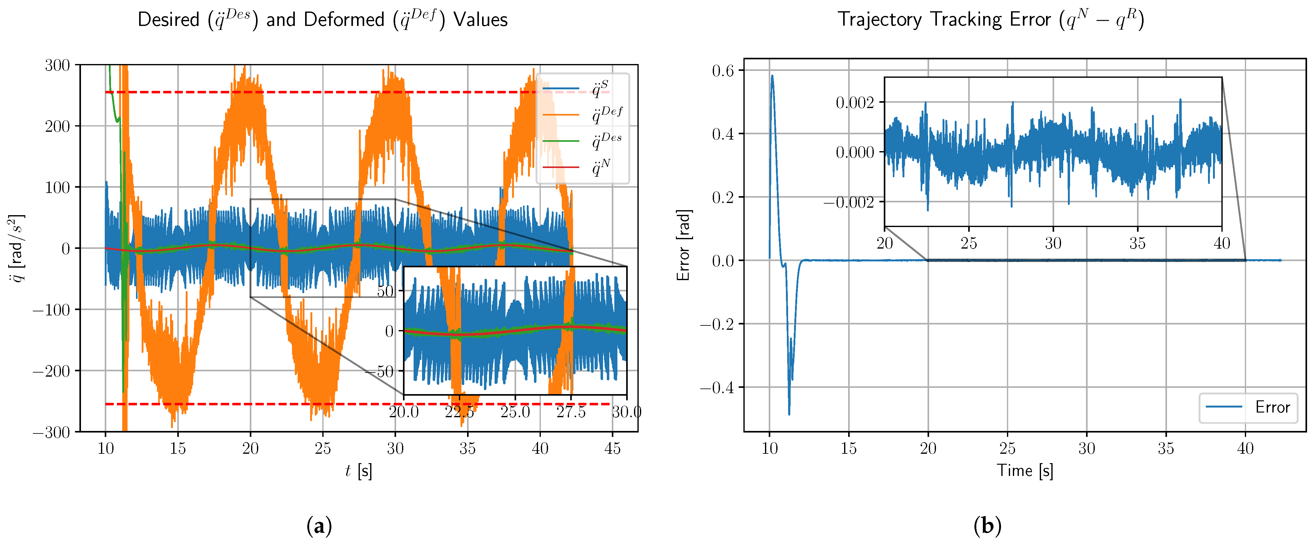
The article is structured in the following manner. In Section 2 some implementation details of RFPT-based control is presented, including the formulation of the kinematic prescription and the adaptive deformation. In this section convergence criteria will be presented as well. Section 3 presents the proposed solution for noise filtering with feedback delay. In Section 4 some simulation and experimental results are presented. Finally, in Section 5 the conclusions are summarized.

2. On the Implementation of RFPT Control

In case of a second-order systems such as industrial robots, the second-order derivatives of the generalized coordinates can be instantaneously set by some control input, i.e., through a force input for linear or through torque for rotational actuators. Meanwhile lower-order derivatives are changing significantly slower. The idea of the CTC method is that by the use of some kinematic prescription the error dynamics is defined, which could be achieved through the implementation of some desired acceleration (${\ddot{q}}^{Des}\left(t\right)$) command. The kinematic prescription is usually defined by a linear control rule and the nonlinear dynamics of the controlled system is decoupled by the use of the inverse dynamic model ($\mathrm{\Psi }(·)$) such as

$$Q\left(t\right)=\mathrm{\Psi }\left({\ddot{q}}^{Des}\left(t\right),{\dot{q}}^R\left(t\right),q^R\left(t\right)\right),$$

(1)

where $Q\left(t\right)$ is the control force, and $q^R\left(t\right)$ is the realized position; finally, ${\dot{q}}^R\left(t\right)$ is the realized velocity of the system. However, in most scenarios the available dynamic model ($\tilde{\mathrm{\Psi }}(·)$) is neither precise nor complete, which gives an approximate control force

$$\begin{array}{cc}\hfill & \tilde{Q}\left(t\right)=\tilde{\mathrm{\Psi }}\left({\ddot{q}}^{Des}\left(t\right),{\dot{q}}^R\left(t\right),q^R\left(t\right)\right),\mathrm{that}\mathrm{results}\mathrm{in}\hfill \end{array}$$

(2a)

$$\begin{array}{cc}\hfill & {\ddot{q}}^R\left(t\right)=\psi \left(\tilde{Q}\left(t\right),{\dot{q}}^R\left(t\right),q^R\left(t\right)\right)\ne {\ddot{q}}^{Des}\left(t\right),\hfill \end{array}$$

(2b)

where $\psi (·)$ is some response function representing the actual dynamics of the controlled system. The idea presented in [16] is that by introducing an appropriate deformation function ($G(·)$)

$$\begin{array}{cc}\hfill & {\ddot{q}}^{Def}\left(t\right)=G\left({\ddot{q}}^{Def}(t-\delta t),{\ddot{q}}^R(t-\delta t),{\ddot{q}}^{Des}\left(t\right)\right),\hfill \end{array}$$

(3a)

$$\begin{array}{cc}\hfill & \widehat{Q}\left(t\right)=\tilde{\mathrm{\Psi }}\left({\ddot{q}}^{Def}\left(t\right),{\dot{q}}^R\left(t\right),q^R\left(t\right)\right),\mathrm{forces}\mathrm{the}\mathrm{system}\mathrm{to}\hfill \end{array}$$

(3b)

$$\begin{array}{cc}\hfill & {\ddot{q}}^R\left(t\right)=\psi \left(\widehat{Q}\left(t\right),{\dot{q}}^R\left(t\right),q^R\left(t\right)\right)\approx {\ddot{q}}^{Des}\left(t\right).\hfill \end{array}$$

(3c)

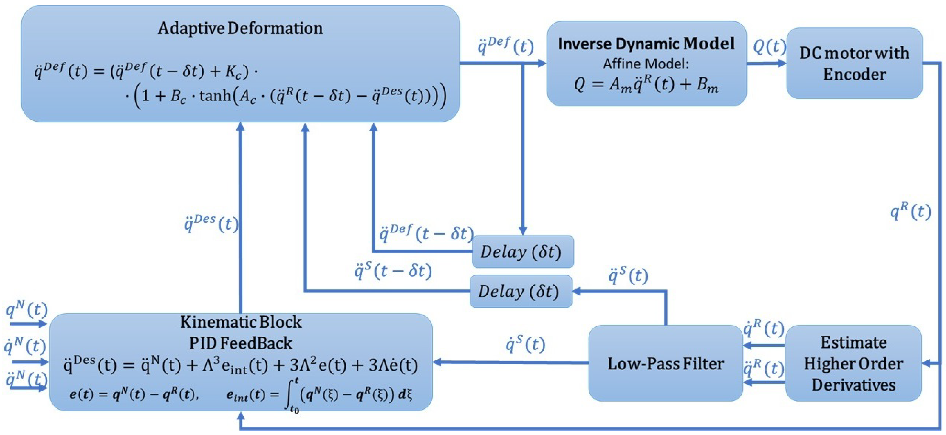
In the RFPT method the approximate control force (3b) is calculated from the deformed second derivative ${\ddot{q}}^{Def}\left(t\right)$ instead of the desired one. In Equation (3) $\delta t$ denotes some feedback delay, which is usually the sampling time of the controller. Figure 1 presents the practical implementation of RFPT-based adaptive controller for a motor control application, where some nominal trajectory $(q^N\left(t\right),{\dot{q}}^N\left(t\right),{\ddot{q}}^N\left(t\right))$ must be precisely followed. In this example the kinematic prescription is defined using simple PID-type error decrease rule, which is among the most commonly used formulations. However, the RFPT method is not limited to this approach; it can also be integrated with alternative control strategies, such as control Lyapunov function-based methods [39] or Backstepping control [40].

2.1. Kinematic Prescription

In case of the CTC method, accurate tracking of the nominal trajectory can be achieved by shaping the error dynamics of the controlled system. A third-order rule for the decrease in the integrated trajectory tracking error ($e_{int}\left(t\right)$) is often employed to achieve robustness against steady-state error and disturbances, i.e., with a constant positive parameter $\mathrm{\Lambda }>0$

$$\begin{array}{cc}\hfill & {\left(\mathrm{\Lambda }+{\displaystyle \frac{\mathrm{d}}{\mathrm{d}t}}\right)}^3{e}_{int}\left(t\right)=0,\mathrm{where}\hfill \end{array}$$

(4a)

$$\begin{array}{cc}\hfill & e_{int}\left(t\right)={\int }_{t_0}^{t}e\left(\tau \right)\mathrm{d}\tau \mathrm{and}e\left(t\right)=q^N\left(t\right)-q^R\left(t\right).\hfill \end{array}$$

(4b)

Equation (4a) expands to a third-order ordinary differential equation of the form

$${\mathrm{\Lambda }}^3{e}_{int}\left(t\right)+3{\mathrm{\Lambda }}^2{\dot{e}}_{int}\left(t\right)+3\mathrm{\Lambda }{\ddot{e}}_{int}\left(t\right)+{\stackrel{⃛}{e}}_{int}\left(t\right)=0.$$

(5)

Equation (5) is obtained from Equation (4a), it must be noted that for differentiable functions the linear operators $\mathrm{\Lambda }$ and ${\displaystyle \frac{\mathrm{d}}{\mathrm{d}t}}$ with a constant parameter $\mathrm{\Lambda }$ commute since

$${\displaystyle \frac{\mathrm{d}}{\mathrm{d}t}}\left(\mathrm{\Lambda }f\left(t\right)\right)=\mathrm{\Lambda }\left({\displaystyle \frac{\mathrm{d}}{\mathrm{d}t}}f\left(t\right)\right),$$

(6)

therefore this algebra is commutative as that defined with the real constant numbers $a,b\in \mathbb{R}$: $(a+b)f\left(t\right)$, therefore the binomial coefficients can be applied in the same form for any $m\in \mathbb{N}$ as

$${\left({\displaystyle \frac{\mathrm{d}}{\mathrm{d}t}}+\mathrm{\Lambda }\right)}^m=\sum _{\ell =0}^m{\displaystyle \frac{m!}{\ell !(m-\ell )!}}{\mathrm{\Lambda }}^{\ell }{\left({\displaystyle \frac{\mathrm{d}}{\mathrm{d}t}}\right)}^{m-\ell }.$$

(7)

It is important to note that this algebra is not as associative as that of the multiplication with real numbers:

$$a\left(bf\left(t\right)\right)=\left(ab\right)f\left(t\right),\mathrm{but}\left({\displaystyle \frac{\mathrm{d}}{\mathrm{d}t}}\mathrm{\Lambda }\right)f\left(t\right)\ne {\displaystyle \frac{\mathrm{d}}{\mathrm{d}t}}\left(\mathrm{\Lambda }f\left(t\right)\right),$$

(8)

that is, the order of multiplications is strictly determined as a direction from right to left. Equation (4a)—that is identical to (5)—corresponds to a linear, time-invariant, homogeneous differential equation with constant coefficients. It is known that any linear combination of two solutions made by the use of constant coefficients is its solution, too. Consequently its solutions form a linear space. Since for each $m\in \{0,\mathbb{N}\}$, for the functions $g_m\left(t\right):={(t-t_0)}^{m}exp(-\mathrm{\Lambda }(t-t_0))$ it holds that

$$\left(\mathrm{\Lambda }+{\displaystyle \frac{\mathrm{d}}{\mathrm{d}t}}\right){(t-t_0)}^{m}exp(-\mathrm{\Lambda }(t-t_0))=m{(t-t_0)}^{m-1}exp(-\mathrm{\Lambda }(t-t_0)),$$

evidently $\left(\mathrm{\Lambda }+{\displaystyle \frac{\mathrm{d}}{\mathrm{d}t}}\right)q_0\left(t\right)\equiv 0$, ${\left(\mathrm{\Lambda }+{\displaystyle \frac{\mathrm{d}}{\mathrm{d}t}}\right)}^2{q}_1\left(t\right)\equiv 0$, and ${\left(\mathrm{\Lambda }+{\displaystyle \frac{\mathrm{d}}{\mathrm{d}t}}\right)}^3{q}_2\left(t\right)\equiv 0$, for constant real $C_0$, $C_1$, and $C_2$ values

$${\left(\mathrm{\Lambda }+{\displaystyle \frac{\mathrm{d}}{\mathrm{d}t}}\right)}^3\left(C_0{g}_0\left(t\right)+C_1{g}_1\left(t\right)+C_2{g}_2\left(t\right)\right)\equiv 0.$$

It is also known that the general solution of a third-order differential equation has three free parameters that are determined by the initial conditions $e_{int}\left(t_0\right)$, ${\dot{e}}_{int}\left(t_0\right)$, and ${\ddot{e}}_{int}\left(t_0\right)$. Therefore the above defined three constants $C_0$, $C_1$, and $C_2$ must determine the general solution. In other words, the exponentially damped functions $g_0\left(t\right)$, $g_1\left(t\right)$, and $g_2\left(t\right)$ as basis vectors span the linear space of the general solutions as

$$e_{int}\left(t\right)=(C_0+C_1(t-t_0)+C_2{(t-t_0)}^2)exp(-\mathrm{\Lambda }(t-t_0)).$$

(9)

Independently of the initial conditions each basis vector converges to 0 as $t\to \infty$, consequently if this kinematically formulated strategy is precisely realized, $e_{int}\left(t\right)\to 0$, $e\left(t\right)\to 0$, and $\dot{e}\left(t\right)\to 0$ as $t\to \infty$. with $C_0=0$, where the values of the $C_1$ and $C_2$ constants depend on the initial conditions. The relationship between the initial conditions and the constant coefficients $C_0$, $C_1$, $C_2$ can be found in a simple recursive manner as follows:

$$\begin{array}{cc}\hfill & g_2\left(t\right)={(t-t_0)}^{2}exp(-\mathrm{\Lambda }(t-t_0)),g_2\left(t_0\right)=0\hfill \\ \hfill & g_1\left(t\right)=(t-t_0)exp(-\mathrm{\Lambda }(t-t_0)),g_1\left(t_0\right)=0\hfill \\ \hfill & g_0\left(t\right)=exp(-\mathrm{\Lambda }(t-t_0)),g_0\left(t_0\right)=1\hfill \end{array}$$

(10)

$$\begin{array}{cc}\hfill & {\dot{g}}_2\left(t\right)=2g_1\left(t\right)-\mathrm{\Lambda }{g}_2\left(t\right),{\dot{g}}_2\left(t_0\right)=0\hfill \\ \hfill & {\dot{g}}_1\left(t\right)=g_0\left(t\right)-\mathrm{\Lambda }{g}_1\left(t\right),{\dot{g}}_1\left(t_0\right)=1\hfill \\ \hfill & {\dot{g}}_0\left(t\right)=-\mathrm{\Lambda }{g}_0\left(t\right),{\dot{g}}_0\left(t_0\right)=-\mathrm{\Lambda }\hfill \end{array}$$

(11)

$$\begin{array}{cc}\hfill & {\ddot{g}}_2\left(t\right)=2{\dot{g}}_1\left(t\right)-\mathrm{\Lambda }{\dot{g}}_2\left(t\right),{\ddot{g}}_2\left(t_0\right)=2\hfill \\ \hfill & {\ddot{g}}_1\left(t\right)={\dot{g}}_0\left(t\right)-\mathrm{\Lambda }{\dot{g}}_1\left(t\right),{\ddot{g}}_1\left(t_0\right)=-2\mathrm{\Lambda }\hfill \\ \hfill & {\ddot{g}}_0\left(t\right)=-\mathrm{\Lambda }{g}_0\left(t\right),{\ddot{g}}_0\left(t_0\right)={\mathrm{\Lambda }}^2\hfill \end{array}$$

(12)

From the above equations the following recursion is obtained:

$$\begin{array}{cc}\hfill & g\left(t\right)=C_0{g}_0\left(t\right)+C_1{g}_1\left(t\right)+C_2{g}_2\left(t\right)\hfill \\ \hfill & C_0=g\left(t_0\right)\hfill \\ \hfill & C_1=\dot{g}\left(t_0\right)+\mathrm{\Lambda }{C}_0\hfill \\ \hfill & C_2={\displaystyle \frac{1}{2}}\left(\ddot{g}\left(t_0\right)-{\mathrm{\Lambda }}^2{C}_0+2\mathrm{\Lambda }{C}_1\right).\hfill \end{array}$$

(13)

Since $\ddot{e}\left(t\right)={\ddot{q}}^R\left(t\right)-{\ddot{q}}^N\left(t\right)$, the desired acceleration command, based on Equation (5), can be chosen as

$${\ddot{q}}^{Des}\left(t\right)={\ddot{q}}^N\left(t\right)+{\mathrm{\Lambda }}^3{e}_{int}\left(t\right)+3{\mathrm{\Lambda }}^{2}e\left(t\right)+3\mathrm{\Lambda }\dot{e}\left(t\right),$$

(14)

where $\mathrm{\Lambda }>0$ is a single design parameter that is equivalent to $K_i={\mathrm{\Lambda }}^3$, $K_p=3{\mathrm{\Lambda }}^2$, and $K_d=3\mathrm{\Lambda }$ PID gains. The ${\ddot{q}}^{Des}\left(t\right)$ should be precisely implemented by controller in order to achieve precise trajectory tracking with exponentially decreasing errors.

2.2. Adaptive Deformation

In the presence of modeling errors the precise implementation of ${\ddot{q}}^{Des}\left(t\right)$ is impossible in a CTC scheme. In RFPT-based adaptive control instead of refining the available dynamic model for a single input–single output (SISO) system a deformation function is introduced such as

$$G({\ddot{q}}^{Def}(t-\delta t),{\ddot{q}}^R(t-\delta t),{\ddot{q}}^{Des}\left(t\right))\stackrel{\mathrm{def}}{=}\left({\ddot{q}}^{Def}(t-\delta t)+K_c\right)\left[1+B_{c}tanh\left(A_c\left({\ddot{q}}^R(t-\delta t)-{\ddot{q}}^{Des}\left(t\right)\right)\right)\right]-K_c={\ddot{q}}^{Def}\left(t\right)$$

(15)

and the deformed value is used to calculate the control force with the initial condition ${\ddot{q}}^{Def}\left(0\right)={\ddot{q}}^{Des}\left(0\right)$. The behavior of this construction becomes mathematically more treatable if on the basis of Equation (3) an approximate “Response Function” for the deformed input is introduced as

$${\ddot{q}}^R\left(t\right)=\psi \left(\tilde{\mathrm{\Psi }}\left({\dot{q}}^R\left(t\right),q^R\left(t\right),{\ddot{q}}^{Def}\left(t\right)\right),{\dot{q}}^R\left(t\right),q^R\left(t\right)\right)\approxeq F\left({\ddot{q}}^{Def}\left(t\right)\right),$$

(16)

in which the “slow drift” of the variables ${\dot{q}}^R\left(t\right)$ and $q^R\left(t\right)$ are neglected. Also, if ${\ddot{q}}^{Des}\left(t\right)$ does not vary in a too hectic manner, it can be written that

$${\ddot{q}}^{Def}(t+\delta t)=G\left({\ddot{q}}^{Def}\left(t\right),F\left({\ddot{q}}^{Def}\left(t\right)\right),{\ddot{q}}^{Des}\left(t\right)\right)\approxeq G\left({\ddot{q}}^{Def}\left(t\right)\right).$$

(17)

The fixed point ${\ddot{q}}_{★}$ satisfies the equation ${\ddot{q}}_{★}=G\left({\ddot{q}}_{★}\right)$. With this the approximation can be written that

$${\ddot{q}}^{Def}(t+\delta t)-{\ddot{q}}_{★}\approxeq G\left({\ddot{q}}_{★}+{\ddot{q}}^{Def}\left(t\right)-{\ddot{q}}_{★}\right)\approxeq G\left({\ddot{q}}_{★}\right)+G^{\prime }\left({\ddot{q}}_{★}\right)\left({\ddot{q}}^{Def}\left(t\right)-{\ddot{q}}_{★}\right)-{\ddot{q}}_{★},$$

(18)

that is

$${\ddot{q}}^{Def}(t+\delta t)-{\ddot{q}}_{★}\approxeq G^{\prime }\left({\ddot{q}}_{★}\right)\left({\ddot{q}}^{Def}\left(t\right)-{\ddot{q}}_{★}\right).$$

(19)

That is, if $\left|G^{\prime }\left({\ddot{q}}_{★}\right)\right|<1$, the sequence converges to the fixed point. This evidently corresponds to Banach’s theorem since it can be written that in the vicinity of the fixed point

$$\left|G\left(x_2\right)-G\left(x_1\right)\right|=\left|{\int }_{x_1}^{x_2}{G}^{\prime }\left(x\right)\mathrm{d}x\right|\le {\int }_{x_1}^{x_2}\left|G^{\prime }\left(x\right)\right|\mathrm{d}x\le max\left(\right|G^{\prime }\left|\right)\left|x_2-x_1\right|,$$

(20)

therefore if there exist $0\le \gamma <1$ so that $\left|G^{\prime }\right|\le \gamma$, a sequence is obtained that converges toward the unique fixed point ${\ddot{q}}_{★}$.

Actually, the function $G(·)$ has two distinct fixed points: one of them is a “false” stationary fixed point that is ${\ddot{q}}^{Def}\left(t\right)=-K_c$, which results in $G(·)=-K_c$. The second one is a “dynamic” fixed point, which evolves with each control iteration. It is only reached when the realized acceleration matches the desired one, such that ${\ddot{q}}^R(t-\delta t)={\ddot{q}}^{Des}\left(t\right)$. Under this condition the adaptive deformation function is $G(·)={\ddot{q}}^{Def}\left(t\right)$. It reflects a moving equilibrium where the control system continuously updates the desired acceleration to match the realized dynamics, ensuring smooth tracking.

Considering that ${\ddot{q}}^R(t-\delta t)=F\left({\ddot{q}}^{Def}(t-\delta t)\right)$ the derivative is expressed as

$$G^{\prime }(·)=\left(1+B_{c}tanh\left(A_c(F(·)-{\ddot{q}}^{Des}\left(t\right))\right)\right)+\left({\displaystyle \frac{({\ddot{q}}^{Def}(t-\delta t)+K_c)B_c{A}_c{F}^{\prime }(·)}{{cosh}^2(A_c(F(·)-{\ddot{q}}^{Des}\left(t\right))}}\right).$$

(21)

It is evident if ${\ddot{q}}^R\left(t\right)$ is in some vicinity of the desired trajectory, i.e., ${\ddot{q}}^R(t-\delta t)\approx {\ddot{q}}^{Des}\left(t\right)\pm ϵ$, then the hyperbolic functions can be approximated simply as ${cosh}^2(·)\approx 1$, $tanh(·)\approx 0$ and by the proper choice of the sign of $B_c$—that depends on $F^{\prime }(·)$—and setting the $K_c$ sufficiently large the iteration is expected to converge. Furthermore, the basin of attraction for the dynamic fixed point is sensitive to the tuning of $A_c$, which governs the steepness of the tanh function and thus the responsiveness of the deformation mechanism to tracking errors. It is important to note that the conditions of convergence normally are valid only within a bounded basin of attraction. The properties of this basin mainly depend on the dynamic properties of the controlled system. In Equation (19) the main factor is the derivative of the response function $F^{\prime }$ that should be either positive or negative in the basin under consideration. In the case of underactuated mechanical systems this property—that in a more general MIMO case was defined as the sign of each eigenvalue of the symmetric matrix ${\left({\displaystyle \frac{\partial F}{\partial {\ddot{q}}^{Def}}}\right)}^T+{\displaystyle \frac{\partial F}{\partial {\ddot{q}}^{Def}}}$—can vary in model-dependent regions. Where this derivative yields zero values the system cannot be controlled, and no any mathematical trick can compensate for this physical property of the controlled system. However, if the system behaves well, and the adaptive control parameters can be set, the controller can enter into a “chaotic regime” that was investigated in detail in [41,42]. This chaotic regime can be left by adjusting the adaptive parameters. It should be noted that in the case of the Lyapunov function-based control design the typical limiting factors normally are listed in the rigorous mathematical formulation of the conditions in the proofs. In the case of dynamic control in practice the nominal trajectory may start from the initial point of the controlled system with slowly increasing velocity, i.e., small initial acceleration that helps keep the controller in the stable basin. (For nonlinear systems the step function-like excitations that normally are applied for the linear models of electrical engineers are not a lucky approach).

2.3. Basic Assumptions in Problem Formulation

Before proceeding with the introduction of the details of the novelties, it is expedient to summarize the basic assumptions in the problem formulation. There are some common assumptions for the simulations and the experiments, and there are special ones only for the simulations, which do not apply to the experimental implementation.

The common assumption is that the iterative adaptive sequence of the deformed signals can converge in the case of the controlled system. This can be concluded from the properties of its dynamic model that provides the “Response Function” in Equation (16). In this simple SISO case that means that ${\displaystyle \frac{\mathrm{d}F}{\mathrm{d}{\ddot{q}}^{Def}}}$ is either positive or negative. Then, according to the detailed considerations it is possible to appropriately set the adaptive control parameters $A_c$, $K_c$, and $B_c$. For multiple input–multiple output (MIMO) systems in [24] this requirement was so generalized that the real part of each eigenvector of the quadratic matrix ${\displaystyle \frac{\partial F}{\partial {\ddot{q}}^{Def}}}$ must be either positive or negative. In [43] these properties were geometrically interpreted as “approximately locally direction keeping” or direction reserving functions as the MIMO generalizations of the monotonic increasing or decreasing functions.

A further tacit common assumption is that the dynamic properties of the nominal trajectory and that of the desired second time-derivatives influenced by the PID type error feedback parameters are not too hectic and allow fast enough convergence for the single adaptive step per one control step adaptation mechanism. This property is important because this adaptive control does not “learn” an exact model: it works on the basis of the freshest available observations.

The assumptions that were made only in the simulations were that the digital controller has a fixed cycle time, and during each control cycle fresh measurement data are available.

3. Modeling Signal Delay at Low Frequency

In life sciences, e.g., in [44], delay effects at low frequency are often modeled with the insertion of a fictitious “ancillary” compartment that does not model a particular, anatomically realistic “organ”. Let $\tau$ [s] model some time delay. Let $u\left(t\right)$ be a noisy signal to be tackled by the use of two compartments, i.e., $S_1\left(t\right)$ and $S_2\left(t\right)$, in which $S_1\left(t\right)$ is directly fed by $u\left(t\right)$, and $S_2\left(t\right)$ is fed by $S_1\left(t\right)$ according to the equations as follows:

$$\begin{array}{cc}\hfill & {\dot{S}}_1\left(t\right)=-{\displaystyle \frac{S_1\left(t\right)}{\tau }}+u\left(t\right)\hfill \end{array}$$

(22a)

$$\begin{array}{cc}\hfill & {\dot{S}}_2\left(t\right)=-{\displaystyle \frac{S_2\left(t\right)}{\tau }}+{\displaystyle \frac{S_1\left(t\right)}{\tau }}\hfill \end{array}$$

(22b)

The above linear operations in the frequency domain using the Laplace transform take the form

$$\begin{array}{cc}\hfill & s{S}_1\left(s\right)=-{\displaystyle \frac{S_1\left(s\right)}{\tau }}+U\left(s\right)\hfill \end{array}$$

(23a)

$$\begin{array}{cc}\hfill & s{S}_2\left(s\right)=-{\displaystyle \frac{S_2\left(s\right)}{\tau }}+{\displaystyle \frac{S_1\left(s\right)}{\tau }}\hfill \end{array}$$

(23b)

that corresponds to a transfer function for $U\left(s\right)$ as

$$S_2\left(s\right)={\displaystyle \frac{(1/\tau )}{(s^2+(2/\tau )s+1/{\tau }^2))}}U\left(s\right)=T\left(s\right)U\left(s\right).$$

(24)

At $s=0$ it yields $S_2\left(0\right)=\tau U\left(0\right)$. The inverse Laplace transform of this signal is

$$\begin{array}{cc}\hfill & S_2\left(t\right)={\displaystyle \frac{1}{2\pi i}}{\int }_{-i\infty }^{+i\infty }exp\left(st\right)T\left(s\right)U\left(s\right)\mathrm{d}s=\hfill \\ \hfill & {\displaystyle \frac{1}{2\pi }}{\int }_{\infty }^{+\infty }exp(i\omega t+i\mathrm{\Phi }\left(i\omega \right))\left|T\left(i\omega \right)\right|U\left(i\omega \right)\mathrm{d}\omega .\hfill \end{array}$$

(25)

If the excitation signal is an element of function class $\mathcal{D}$, i.e., it has a finite support and it can be continuously differentiated infinitely many times (e.g., [45]), around $\omega =0$ where $\left|T\right(i\omega \left)\right|\approxeq \tau$, $S_2\left(t\right)$ can be approximated as

$$S_2\left(t\right)\approxeq {\displaystyle \frac{\tau }{2\pi }}{\int }_{-\infty }^{+\infty }exp(i\omega t+i\mathrm{\Phi }\left(i\omega \right))U\left(i\omega \right)\mathrm{d}\omega .$$

(26)

The signal delayed by $\delta t>0$, i.e., $u(t-\delta t)$ in the frequency domain can be computed as

$$u(t-\delta t)={\displaystyle \frac{1}{2\pi }}{\int }_{-\infty }^{+\infty }exp(i\omega t-i\omega \delta t)U\left(i\omega \right)\mathrm{d}\omega .$$

(27)

By comparing these equations it can be seen that this signal tackling means a delay

$$\delta t=-{\displaystyle \frac{\mathrm{\Phi }\left(i\omega \right)}{\omega }}.$$

(28)

Note that after elapsing the contribution of the initial state, in the noise filter only the effects of the persistent excitation can be considered. No any complementary assumption is needed to arrive at Equation (28) from Equation (25): only mathematical analogies are physically interpreted in the following manner. Assume that $U\left(\omega \right)\in \mathcal{D}$ has only a very narrow support around a value ${\omega }_a$ as $[{\omega }_a-\Delta ,{\omega }_a+\Delta ]$. This means that the excitation has a fixed frequency. For a function $T\left(s\right)$ that is continuous along the route of integration (it has poles only in one half of the complex plane) the integral ${\int }_{-\infty }^{\infty }$ can be reduced to ${\int }_{{\omega }_a-\Delta }^{{\omega }_a+\Delta }$, and the integral can be estimated as $|T\left(i{\omega }_a\right)|{\int }_{{\omega }_a-\Delta }^{{\omega }_a+\Delta }exp(i\omega t+i\mathrm{\Phi }\left(i{\omega }_a\right))U\left(i\omega \right)\mathrm{d}\omega$. In this case $\mathrm{\Phi }\left(i{\omega }_a\right)$ is the “phase shift” that according to Equation (27) corresponds to a delay. In other words, the LTI system that is excited with a fixed frequency signal, after elapsing the effects of the initial conditions, moves with the frequency of the excitation with an attenuation factor and a phase shift. The technical literature always considers the “phase shift” due to the traditions made by Bode’s work [46] and does not mention that the phase shift physically means a delay. For non-monochromatic excitation the output signal is deformed because its various frequency components are attenuated and delayed in various manners.

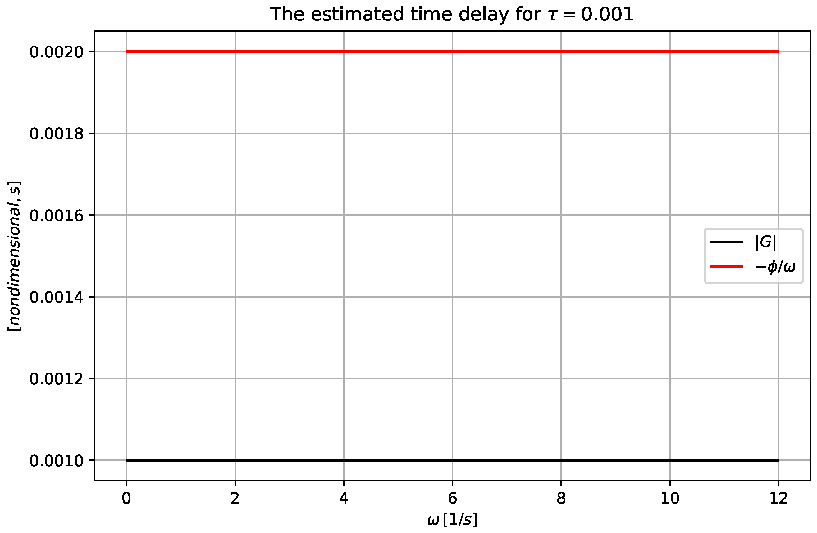
In the motion control of mechanical systems for a fast motion the upper frequency limit is approximately $\Omega =12.0\left[s^{-1}\right]$, for which a delay $\tau ={10}^{-3}$ [s]; the low frequency transfer function is depicted in Figure 2.

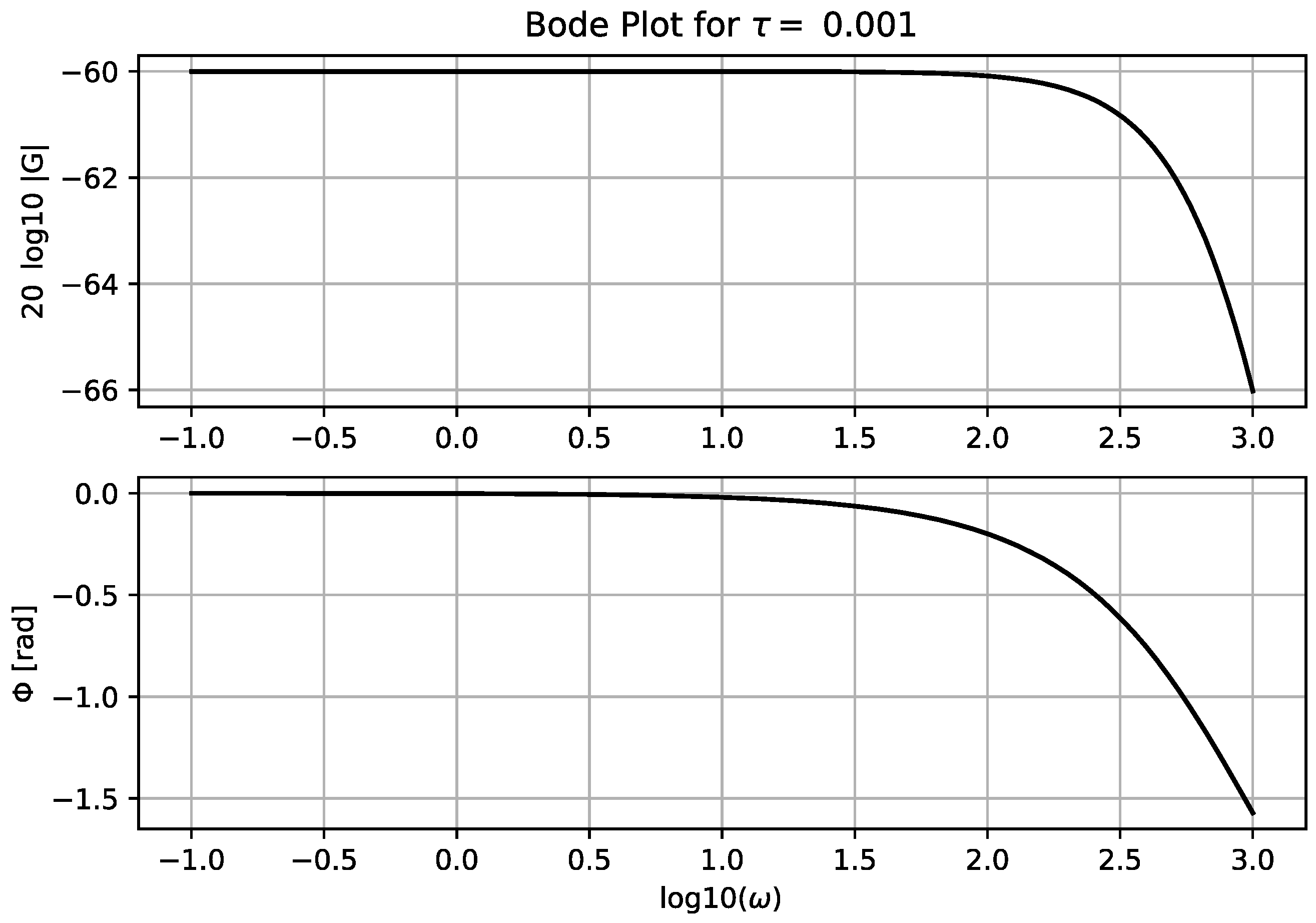
The transfer function for higher frequencies are depicted in the Bode plot, Figure 3.

While in our previous investigations the issues of noise filtering and delay were considered separate issues, i.e., certain noise filtering techniques were applied and the filtered signal was sampled with some exact delay, in the present approach the low frequency delay was utilized and the high frequency filtering, as an additional service, was directly utilized too, as in

$$f(t-2\tau )\to {\displaystyle \frac{S_2\left(t\right)}{\tau }}.$$

(29)

In this way, the cumulative effects of noise filtering and formal delay could be avoided in the FPI-based control. Furthermore, while the formally applied delay time must be very precisely specified in the calculations, this smeared delay has a noticeable effect even slightly later in time, making the adaptive method based on it more robust. Such effects were investigated in the sequel.

It is important to note that this filtering and delaying model is exactly valid in the application and it is independent of the dynamic model of the controller. Also, in the control process it is utilized in the time domain via numerical integration. For the composite array $x\left(t\right):={\left[S_1\left(t\right),S_2\left(t\right)\right]}^T$ its equation of motion has the standard “canonical form” of $\dot{x}\left(t\right)=Ax\left(t\right)+Bu\left(t\right)$ with constant matrices $A=\left[\begin{array}{cc}{\displaystyle \frac{-1}{\tau }}& 0\\ {\displaystyle \frac{1}{\tau }}& {\displaystyle \frac{-1}{\tau }}\end{array}\right]$ and $B=\left[\begin{array}{c}1\\ 0\end{array}\right]$ and the general solution of this equation of motion has the form

$$x\left(t\right)=exp\left(A(t-t_0)\right)x\left(t_0\right)+{\int }_{t_0}^{t}exp\left(A(t-\zeta )\right)Bu\left(\zeta \right)\mathrm{d}\zeta ,$$

(30)

with a stable matrix. The first term is the general solution of the homogeneous equation $\dot{x}=Ax$ that contains the initial conditions at $t_0$, the second one is a particular solution of the inhomogeneous one. Due to the stability of the system the first term converges to zero, therefore its significance soon elapses. The second term corresponds to a persistent excitation that evidently contains delayed effects from the past. In the frequency domain only the effect of this persistent part was investigated in order to distinguish between the delays pertaining to the low frequency and the high frequency components of the excitation.

4. Application in FPI-Based Adaptive Control

The block diagram of the RFPT-based adaptive control was presented in Figure 1 and was implemented with the proposed double counterpart model in both the simulation- and experiment-based investigations. The noisy measured $q^R$, ${\dot{q}}^R$ signals are filtered with a double counterpart model using $\tau ={10}^{-3}$ [s] in the PID-type tracking strategy, while ${\ddot{q}}^R$ observed realized a second time-derivative and the ${\ddot{q}}^{Def}$ deformed values are filtered with a similar double compartment model with delay $2\tau$, while ${\ddot{q}}^{Des}$ is calculated without any delay. In both investigations the approximately constant multiplication is taken into account, too. Essentially the exact “Delay” blocks with the double counterpart model are replaced. With the above method the adaptive controller works well.

4.1. Simulation Results

In the Introduction, several factors (the operation and the parallel tasks of the operating system, interrupts-based processing of the sensor signals, delay in the control electronics) were mentioned due to which the simulations cannot be made realistic enough to completely mirror the reality. For this reason a 100% agreement between the measurements and the simulations cannot be expected. However, it can be shown that the effects of the neglected subtle details do not cause significant differences between the simulations and the measurements. For this reason, for the simulation a more complex dynamical system (the van der Pol oscillator) than the simple one for which the experimental test system was built up was chosen. The properties of the so-obtained simulation results are in harmony with that of the measured ones that are presented in this section. A van der Pol Oscillator modeled in [47] with a dynamic equation

$$\ddot{q}={\displaystyle \frac{-kq+b_1\left(a^2-q^2\right)\dot{q}-b_2\dot{q}+Q}{m}},$$

(31)

in which $Q\left[N\right]$ denotes the control force, k [N/m] is the linear spring stiffness, $a$ [m] the limit value separating the damped/excited operations, $b_1$ [N· s/m³] and $b_2$ [N· s/m] are damping parameters, and $q$ [m] is the generalized coordinate, that is, the expansion of the spring. For simulation purposes a formally exact model with some parametric uncertainty is used, which is shown in

Table 1. The parameters of the van der Pol oscillator.

Parameter	Approximate Value	Exact Value
Spring stiffness $k$ [N/m]	$100.0$	$150.0$
Separator $a$ [m]	$1.0$	$1.2$
Damping/Excitation coefficient $b_1$ [N · s/m3]	$1.0$	$1.5$
Damping coefficient $b_2$ [N · s /m]	$2.0$	$2.5$
Mass $m$ [kg]	$1.0$	$1.5$

.

In the simulations the controller was tuned by the trial-and-error method trying to achieve the best control performance. The design parameter for the kinematic prescription was set to $\mathrm{\Lambda }=16$ [s⁻¹]; meanwhile, the adaptive parameters were $K_c={10}^5$, $B_c=-1$, and $A_c={\displaystyle \frac{0.9}{K_c}}$. The sampling time of the controller was $\delta t=0.001$ s. At first noise-free simulations are presented. Figure 4 shows the evolution of the generalized coordinates and its various derivatives in case of a trajectory tracking application with a sinusoidal nominal trajectory. The delay effect of the double counterpart model is presented here as well. The delay can be observed in the first- and in the second-order derivatives. Figure 4d nicely presents the essence of the RFPT-based control method. The deformed values ${\ddot{q}}^{Def}\left(t\right)$ are significantly different from the desired one (${\ddot{q}}^{Des}\left(t\right)$), which suggests major adaptive deformation due to model errors. However, the realized trajectory ${\ddot{q}}^R\left(t\right)$ nicely follows the desired one as it would be required in the CTC method.

Figure 5 presets the applied control force and the trajectory tracking error for the same simulations, complemented by some additional results without the counterpart delay model for the same parameter settings. As far as the simulation without the feedback delay is considered, after some transient overshoot with maximum error $\widehat{e}\approx 0.274$ m, the “steady-state” maximum tracking error was ${\widehat{e}}_{ss}\approx 0.082$ m. Under these conditions the proposed counterpart delay model improved the control performance as lower initial overshoot ($\widehat{e}\approx 0.147$ m) and maximum “steady-state” error (${\widehat{e}}_{ss}\approx 0.025$ m) can be observed. However, in the initial stage of the control regime, few oscillations can be observed in the control force in the case of the counterpart feedback delay model.

In the next simulations some noise was added to the coordinate measurement. It was simulated as a random signal with normal distributions that have a standard deviation of ${\sigma }_n=5\times {10}^{-4}$. The simulation results with the same parameter settings are presented in Figure 6. Although the noise does not seem that significant in the position measurement, higher derivatives are majorly affected, especially the acceleration signal that is the most critical in the case of RFPT-based adaptive control. However, as the counterpart delay model is fitted in the feedback loop, good noise attenuation was achieved, which is presented in Figure 6b,c. The same issues can be observed in case of the deformed signal due to the feedback of the second-order derivative of the generalized coordinates. However, with the application of the counterpart delay model, sufficiently smooth acceleration command (${\ddot{q}}^{SDef}\left(t\right)$) was achieved, which is presented in Figure 6d. Overall, similar trajectory tracking error was achieved in the case of the measurement noise that was presented previously. The trajectory tacking error shown in Figure 6e has similar characteristics to the noise-free case.

4.2. Experimental Results

The proposed solution was experimentally verified in a DC motor control application. The experimental setup is presented in Figure 7. The control algorithm was implemented on an ARM Cortex-M7 microprocessor, which was driving an FIT0185 12V DC motor, through a BTS7960 chip-based dual half bridge drive. The parameters of the motor—which are available from the manufacturer—are presented in

Table 2. FIT0185 DC motor technical parameters.

Parameter	Nominal Value
Operating Voltage $U_N$ [V]	12
No-load speed $N_0$ [RPM]	$83\pm 10\%$
No-load Current $I_0$ [mA]	350
Start Voltage $U_0$ [V]	$21.0$
Stall Torque $T_s$ [kg· cm]	$45.0$
Stall Current $I_s$ [A]	$7.0$
Gearbox Ratio r	1:131
Encoder Resolution $n$ [CPR]	2096

.

The control algorithm was implemented as presented in Figure 1. In the place of “Low-Pass Filter”, blocking the double counterpart delay model was implemented so the filtered values ${\ddot{q}}^S$, ${\dot{q}}^S$ were obtained from noisy signals that were estimated using second-order backward difference estimation formulae

$$\begin{array}{cc}\hfill & {\dot{q}}^R\left(t\right)={\displaystyle \frac{3q^R\left(t\right)-4q^R(t-\delta t)+q^R(t-2\delta t)}{2\delta t}},\hfill \end{array}$$

(32a)

$$\begin{array}{cc}\hfill & {\ddot{q}}^R\left(t\right)={\displaystyle \frac{2q^R\left(t\right)-5q^R(t-\delta t)+4q^R(t-2\delta t)-q^R(t-3\delta t)}{\delta t^2}}.\hfill \end{array}$$

(32b)

The position measurement $q^R\left(t\right)$ was obtained from the inbuilt encoder of the DC motor with quadrature decoding. The double counterpart delay model parameter was set to $\tau =5\delta t$, where $\delta t$ was the sampling time of the controller that was $0.001$ s. The kinematic prescription was formulated according to Equation (4a) with $\mathrm{\Lambda }=15$ s⁻¹. The deformed signal was obtained from the adaptive deformation function (16) with parameters $B_c=1$, $K_c={10}^6$, and $A_c={\displaystyle \frac{0.6}{K_c}}$. As detailed specification of the motor was not available a simple affine model was used by the controller

$$Q\left(t\right)={\left.\left(A_m{\ddot{q}}^{Def}\left(t\right)+B_m)\right)\right|}_{A_m=1,B_m=0}={\ddot{q}}^{Def}\left(t\right),$$

(33)

that was directly used to calculate the PWM output of the controller as

$$PWM=\left\{\begin{array}{c}255\mathrm{if}\left|Q\left(t\right)\right|>255\hfill \\ \left|Q\left(t\right)\right|\mathrm{if}-255\le Q\left(t\right)\le 255\hfill \end{array}\right..$$

(34)

Essentially Equation (33) corresponds to a “quasi” model free controller, where all the modeling imprecisions are compensated by the adaptive deformation.

Measurement results with the DC motor for the load-free case is presented in Figure 8. The effect of the quantization error is shown in Figure 8a, where the resolution of the encoder is clearly reflected. This caused significant estimation errors in higher derivatives (Figure 8b,c). However, the proposed double counterpart delay model effectively attenuates the quantization noise in the higher derivatives and after a short settling time precise position and velocity tracking were achieved, as shown by the phase trajectory in Figure 8d.

In Figure 9a the red dashed horizontal lines show the actuator limits. In the beginning of the control, excessive control force is observed that is well beyond the actuator limits due to the insufficient initial conditions. The controller introduced significant adaptive deformation throughout the full control regime due to the imprecise control model. However, after a few oscillations precise tracking was achieved as presented in Figure 9b. In the “steady-state” ${\widehat{e}}_{ss}\approx 0.002$ rad maximum tracking error was measured in the case of the $q^{Res}=0.00075$ rad encoder resolution, with the quadrature decoding taken into account.

In the next measurements a spring was fitted on the motor’s shaft in order to introduce external disturbance forces into the system. The spring’s stiffness was $k=0.822 {\displaystyle \frac{\mathrm{N}}{\mathrm{mm}}}$. The results are presented in Figure 10. The deformed signals that are slightly different for the loaded case are as shown in Figure 10a. It can be observed that the deformed signal nicely compensates for the loading torques caused by the spring. The trajectory tracking error presented in Figure 10b has similar characteristics as of the unloaded case. In the “steady-state” ${\widehat{e}}_{ss}\approx 0.003$ rad the maximum tracking error was measured for the spring-loaded motor, which is similar to the unloaded case.

5. Conclusions

RFPT-based adaptive control is prone to noise sensitivity due to the feedback of the second-order derivative of the generalized coordinates in case of a second-order system. In most practical applications for a mechanical system, the position is measured through digital encoders that introduce quantization errors in the measurements. That corrupts the estimation process of higher-order derivatives resulting in significant noise content in the feedback signals. In this paper this issue was tackled by a double counterpart delay model borrowed from life science applications, where it is used to model signal delays without modeling any particular organ. In previous investigations of the RFPT Control method the issues of noise filtering and delay were considered formally separated issues, i.e., certain noise filtering techniques were applied for the signals, and the filtered signals were sampled with some exact delay. In this approach the inevitable delaying effect of the noise filtering technique was not taken into account, and it had an accumulated effect with that of the formally delayed sampling. With this method the adaptive controller works well. This statement was illustrated by both experimental and simulation-based analysis.

Simulations were carried out with a simple van der Pol oscillator model where only parametric uncertainty was considered. It was shown that instead of using some exact delay in signal sampling the proposed controller combined with double counterpart delay model has more robust behavior. Under the investigated conditions the controller had improved trajectory tracking performance with lower error, when the noise-free case was considered. Experimental analysis on a DC motor has shown good noise attenuation in both the first- and second-order derivatives of the generalized coordinates without significantly limiting the responsiveness of the controller. The modeling imprecisions were nicely compensated by the controller and precise trajectory tracking was achieved, even when disturbance forces were introduced in the form of a spring connected to the motor’s shaft.