Abstract
This paper presents a hybrid adaptive control strategy for upper limb rehabilitation robots using impedance learning. The hybrid adaptation consists of a differential updating mechanism for the estimation of robotic modeling uncertainties and periodic adaptations for the online learning of time-varying impedance. The proposed hybrid adaptive controller guarantees asymptotical control stability and achieves variable impedance regulation for robots without interaction force measurements. According to Lyapunov’s theory, we proved that the proposed impedance learning controller guarantees the convergence of tracking errors and ensures the boundedness of the estimation errors of robotic uncertainties and impedance profiles. Simulations and experiments conducted on a parallel robot validated the effectiveness and the superiority of the proposed impedance learning controller in robot-assisted rehabilitation. The proposed hybrid adaptive control has potential applications in rehabilitation, exoskeletons, and some other repetitive interactive tasks.
1. Introduction
Comfort and safety are of significant value in robot-assisted rehabilitation and can be improved through robot impedance regulation. As a well-known compliance control approach, impedance control has shown its powerful abilities in robot impedance regulation and has been extensively applied in service robots and industrial robots [1,2,3,4]. However, robot modeling uncertainties and human impedance variation bring in difficulties for impedance control implementation in rehabilitation training.
Robot modeling uncertainties affect the control stability and the control robustness of impedance control. Up to now, considerable research attention has been paid to robust impedance control [5], adaptive impedance control [6,7], neural impedance control [8,9,10,11], and iterative learning impedance control [12]. These impedance control methods improve the stability and robustness of closed-loop control systems; however, these methods mainly focus on constant impedance regulation.
In robot-assisted rehabilitation, human impedance varies along with the variation in interaction forces and tasks. Time-varying impedance control [13] has better robustness and compliance in rehabilitation training through robotic variable impedance regulation, in comparison with constant impedance control [14,15,16]. Although categories of variable impedance control methods were designed for robot-assisted rehabilitation [17], many of these results neglected the stability of the desired variable impedance dynamics (DVID) which is of significant value for human–robot cooperative motion. Actually, the DVID are described by linear time-varying systems and may be violated by the variation in impedance profiles. In [18], the stability region of impedance parameters was evaluated experimentally for the DVID with zero stiffness. In [19], an adaptive variable impedance controller was designed for force tracking in interaction with an unknown environment with constant impedance. In [20,21,22], novel constraints on time-varying impedance profiles were proposed to guarantee the stability of the DVID, but how to design impedance profiles in robot-assisted rehabilitation was not given in these results.
Designing appropriate impedance profiles to balance between the desired control stability and the desirable interaction performance is of significant value for robot-assisted rehabilitation. For impedance profile construction, the algorithms of Learning from Demonstration and sEMG-based Dynamic Movement Primitives (DMPs) were applied for time-varying impedance control in physical HRI. In [23,24,25], two-loop-based optimal admittance controllers were proposed for robot-assisted rehabilitation. An inner-control loop makes robots behave in a prescribed impedance model, and an outer-loop optimal control aims at finding the optimal parameters of the prescribed impedance model by minimizing a performance function of interaction forces and tracking errors. Almost all impedance/admittance controllers mentioned above were designed using interactive forces; however, the force measurements may become impossible without related force sensors or ineffective due to measurement delay or noises.
From the above analysis, the variable impedance regulation of robots can improve human–robot interactive performances, but impedance variation brings in control stability problems. Recently, model-based impedance learning controllers were proposed in [26,27,28] for human–robot interaction with a control stability guarantee and without the requirement of interaction forces. Specifically, human impedance uncertainties were estimated by using the periodicity characteristics of task reference trajectory and human impedance profiles in [26,27], and an adaptive impedance learning controller was proposed in [28], where robot modeling uncertainties and human impedance uncertainties were estimated by using traditional differential updating laws. However, the results in [26,27,28] have the following deficiencies: (i) these adaptive impedance learning controllers only guarantee the closed-loop control systems be uniformly ultimately bounded (UUB) but not be asymptotically stable; (ii) precise knowledge about robotic dynamic parameters is required in [26,27]; and (iii) the result in [28] requires the unknown impedance profiles be slowly varying due to the weakness of differential adaptation in estimating time-varying signals.
In this paper, we propose an impedance learning-based hybrid adaptive control strategy with potential applications in repetitive rehabilitation training. In comparison with the related literature, the innovations and contributions of this paper are stated as follows:
(1) A differential updating mechanism is designed for estimating robotic parameter uncertainties, while periodic adaptive learning laws are designed for the learning of human time-varying impedance profiles.
(2) The projection function used in the adaptive law and the saturation functions in the periodic adaptive laws avoid the possible drift of estimators.
(3) The proposed hybrid adaptive robot controller guarantees asymptotical control stability and achieves variable impedance regulation for rehabilitation robots without interaction force measurements.
(4) The asymptotical convergence of tracking errors and the finiteness of the estimation errors of the robot parameters and the human impedance profiles are validated through a Lyapunov-like analysis.
Compared with the constant impedance control, the proposed impedance learning-based controller can provide time-varying impedance regulation for rehabilitation robots. In comparison with the impedance learning controllers in [13,18,19,20,21,22], the proposed model-based impedance learning controller can guarantee the control stability without using interaction force signals. Compared with the model-based impedance learning controllers in [26,27,28], the proposed controller guarantees the asymptotical convergence of tracking errors. In addition, robotic parameter uncertainties are considered and estimated in this paper in comparison with [26,27], and the impedance profiles are not required to be slowly varying in comparison with [28]. A summary of currently used adaptive controllers with impedance regulation and the gap where this paper is located are listed in Table 1.

Table 1.
A summary of the currently used adaptive controllers with impedance regulation in rehabilitation.
2. Problem Formulation
Consider the robot dynamics with the following form
where denotes the vector of joint angles, the inertial matrix, the Coriolis and centrifugal matrix, the gravity torque, and the viscous force with being a constant matrix. In (1), and are the interaction force vector in joints and the system control input, respectively.
Denote as the end-effector Cartesian position. The robot has the following kinematic transformations
In (3), is the Jacobian matrix from the joint space to the Cartesian coordinates. Based on (2) and (3), one can convert the joint space dynamics in (1) into the following Cartesian dynamics
where , , , , , and .
Property 1.
is a symmetric positive definite matrix and satisfies
where , and and can be regarded as the minimum and maximum eigenvalues of , respectively.
Property 2.
is skew symmetric, i.e.,
Property 3.
The left part of (4) can be parameterized in the following form
where , is a regression matrix, and θ is a constant vector that contains unknown parameters and satisfies .
Property 4.
If , then and their partial derivatives with respect to their respective arguments are bounded. If , , and its partial derivatives with respect to its arguments are bounded.
Assumption 1.
Suppose the desired trajectory and its first and second time derivatives are bounded for the considered robot in the HRI.
Define the trajectory tracking error e as
As proven in [26], the interaction force can be expanded as
where denotes the feedforward force of the human, and and denote the stiffness term and the damping term of the interaction force, respectively. The interaction force can be further expressed as
where : = denotes a modified feedforward force. In repetitive rehabilitation training, the impedance profiles , and can be assumed to be periodic with , i.e.,
It is assumed that and are continuous functions and satisfy
where , , and are constant matrices; ‘’ in the last equation means each element of the left part of ‘’ is no more than the related element of the right part of ‘’.
Remark 1.
In [25], the feedforward force, the stiffness term, and the damping term are assumed to be slowly varying and are estimated by using traditional adaptive laws. In this paper, , , and are only required to be continuous and bounded functions that will be estimated in Section 3 using periodic adaptation.
3. Hybrid Adaptive Control via Impedance Learning
Define the auxiliary error as
where .
From (4), has the following dynamics
It is convenient to design the following control law
where and are estimators of and , respectively; is designed as
with , , and being estimators of , , and , respectively.
Substituting (11) and (12) into (10) yields
where , , and denote estimation errors.
In (15), is a constant vector that can be estimated by the sing traditional differential updating mechanism, while the impedance profiles , , and are time-varying signals that may not be slowly varying and cannot be effectively estimated using traditional adaptive laws. By exploiting their periodicity characteristics, the impedance profiles can be estimated by using periodic adaptations. Therefore, we propose a hybrid adaptive law for estimating and the impedance profiles.
For , we design the following adaptive update law
where is the learning rate, and is a projection function defined as
with being defined in Property 3.
To estimate the time-varying terms , , and , we design the following periodic learning laws
where , and for ; and are positive gains; , , and are a continuous and strictly increasing function that satisfy , , , and ; is defined by
and , are defined similarly to the definition of .
Based on (12), (13) and (21)–(23), the estimation errors , and , satisfy
for .
Remark 2.
If , , and , then the impedance profile estimators , , and will be discontinuous at with = 0, 1, 2, · · ·, just as the impedance profile estimators in [26,27]. In this paper, the designed , , and in (21)–(23) guarantee the continuity of the impedance profiles estimators at with = 0, 1, 2, ⋯.
Theorem 1.
For the robot dynamics in (1), design the periodic adaptive control strategy in (16), where is updated by the differential type updating law in (19), and , , and are updated by the periodic adaptive laws in (21)–(23). Then, the estimation errors , , , and are uniformly bounded, and the tracking error converges to zero.
Proof.
As and are with differential dynamics and , , and are with periodic difference update learning laws, it is convenient for us to consider the following non-negative function
where , , , and are chosen as
with .
with for . □
i. Finiteness of on
Since , , , and are continuous functions, the righthand side of Equation (15) is continuous. According to the existence theorem of differential equation, there exists a finite solution to (15) in an interval with . It is obvious that is finite on the interval . In the following, we will show the finiteness of on , where , , and . Taking the time derivative of for and substituting (18), one can obtain
The used projection modification in (20) guarantees the following: (1) for ; (2) From the definitions of and we have the following inequalities [29,30]: and Substituting these results into (31), one obtains
for .
From (21)–(23), , and for
Applying these equations into (32) yields
for where
Using Young’s inequality,
where are chosen positive constants, such that
From inequalities in (33)–(36),
where is defined as
From (38), is negative-definite outside the following region
Furthermore, is bounded from the projection modification (20). Therefore, is bounded on .
ii. Convergence of e
For , the time derivatives of and satisfy
Substituting (29) and into (42),
Similarly, one obtains
Since and , from and (41)–(45),
from which one can obtain for and
From the above analysis, for which implies and Combining and one can obtain and based on Property 4. Based on and (21)–(23), . Therefore, the righthand side of (18) is bounded and then which shows that is uniformly continuous in . Babalat’s Lemma can be conducted to show that which implies
Remark 3.
The proposed impedance learning control method requires that the human impedance profiles are temporally periodic, and the robotic dynamics can be linearly parameterized. If any of these requirements are not satisfied, the proposed control method cannot be implemented.
Remark 4.
The hybrid adaptive impedance learning control can provide variable impedance regulation for repetitive robot-assisted rehabilitation without the requirement of the interactive force sensing.
Remark 5.
In applications, control parameters can be selected step by step. Firstly, PD control gains k1 and k2 are adjusted to make the closed-loop control system stable. Secondly, the adaptive learning rate α0 is designed to make the robot follow the reference trajectory with satisfactory tracking accuracy in the case of no human–robot interaction. Next, periodic learning parameters for time-varying impedance are set. Finally, the control parameters are further fine-tuned to achieve satisfactory interactive performances. Under the proposed hybrid adaptive control strategy, the human–robot system follows the reference trajectory cooperatively and repetitively.
4. Simulations
The planar five-bar parallel mechanism depicted by Figure 1 with the structure in Figure 2 is considered as the mechanism for some upper limb rehabilitation robots and is adopted here for simulation validation. To show the effectiveness of the proposed hybrid adaptive control (HAC) and its advantages in comparison with the adaptive control (AC) in [28] and the biomimetic adaptive control (BAC) in [26,27], simulations are conducted on a planar parallel robot depicted by the render graph in with a five-bar parallel.
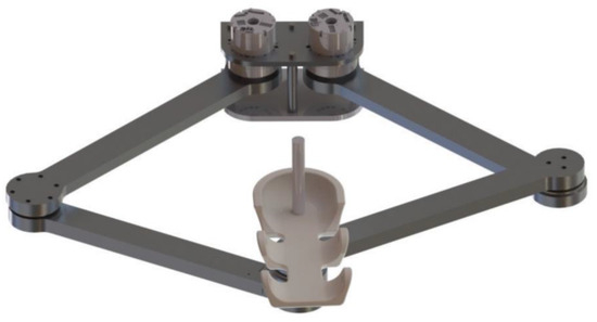
Figure 1.
The render graph of a planar parallel robot.
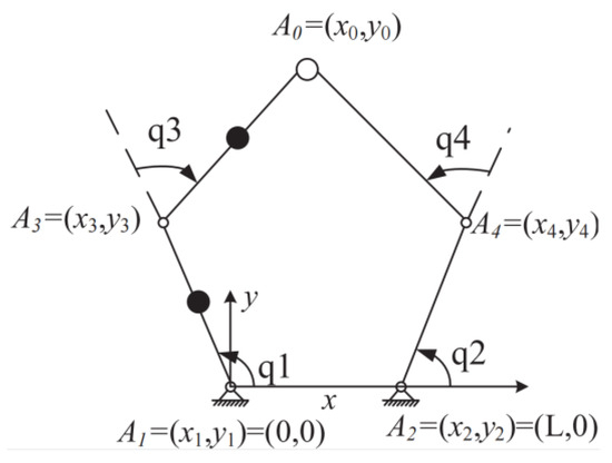
Figure 2.
The robotic structure diagram.
In Figure 2, are the five joint points, where is the HRI point, and , denote four robotic links whose masses, lengths, and inertial moments are given in Table 2. The distances between the joints and respective centers of mass are all 0.25 m, i.e., for and the length of is. In addition to its advantages over a series mechanism, a parallel mechanism results in a more complex model for the robot. In robot-assisted rehabilitation, the reference trajectory is .

Table 2.
The parameters of the parallel robot.
The feedforward force, the stiffness matrix, and the damping matrix are
For the proposed HAC, we choose the following control parameters: In the PD control, the proportional control parameters are determined according to the requirements for the response speed and the static speed error based on the transfer function of the robot model, and the derivative control parameters are designed based on the regulation time and overshooting. Then, the hybrid adaptive learning parameters are determined by trial and evaluation to obtain satisfactory interactive performance.
Figure 3a shows the tracking performance by the proposed HAC, the AC in [28], and the BAC in [26,27] with locally enlarged parts shown in the right part of the figure. From Figure 3a, we can see that the actual trajectory (AT) and the desired trajectory (DT) are almost coincident after several periodic motions using the proposed method, while the AT consistently deviates from the DT using the AC in [28] and the BAC in [26,27]. To better display the effectiveness and advantages of the proposed control method, comparisons of tracking errors among the three methods are illustrated in Figure 3b. It can be seen that the HAC makes the tracking error converge to zero, while the AC in [28] and the BAC in [26,27] only make the tracking error be bounded. The not satisfactory tracking performance by the AC is mainly due to the limitations of traditional differential adaptation in estimating time-varying signals. The better tracking performance validates the superiority of the HAC in comparison to the BAC in [28].
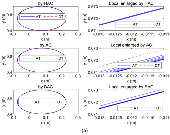
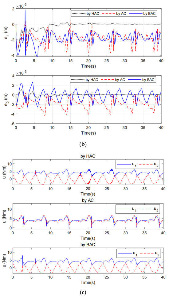
Figure 3.
Simulation performances by the proposed HAC, the AC in [28], and the BAC in [26,27]. (a) The tracking performance, (b) The tracking error, (c) The control input.
It should be noted that the estimated force cannot be very close to the actual interactive force (see Figure 4a) due to the strong coupling between robot modeling uncertainties and human impedance uncertainties. Such derivation is allowable and does not affect control performance shown in Figure 3. In addition, the stiffness and damping variation is finite, which is illustrated by Figure 4b.
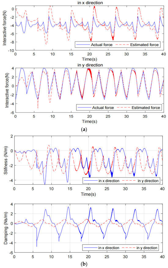
Figure 4.
The estimation of the interactive force and the estimated stiffness and damping by the proposed HAC. (a) Interactive force estimation, (b) Stiffness and damping.
5. Experiments
To further verify the effectiveness and validity of the proposed control method, experiments are implemented on the self-designed planar five-bar parallel mechanism (see Figure 5) which was driven by rotary actuators (erob80, ZeroErrInc., Beijing, China).
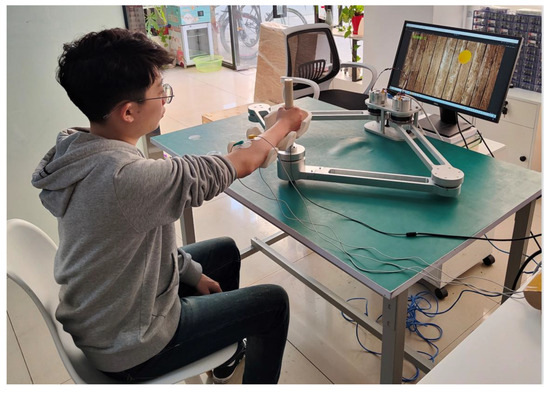
Figure 5.
Physical HRI.
Twincat 3.0 eXtended automation engineering running on a PC acts as the fieldbus master in the EtherCAT network. The control algorithm is implemented by the TwinCAT Component Object Model (TcCOM) programed in structured Text (ST) languages. Both the control frequency and the sampling period for the controller are 1 ms. The rotary actuator is operated in torque mode. The planar parallel robot used in our study is an end-effector rehabilitation robot. The trajectory of the robot is usually predefined by therapists during rehabilitation training. During the rehabilitation process, the patient’s upper limbs are trained with the help of a rehabilitation robot, as in Figure 5. The emerging interactive forces between subjects and the robot may give rise to trajectory deviation for the robot. The proposed impedance learning control can make the human robot system cooperatively follow the desired trajectory. In the experiment, the robot and a subject repetitively track an ellipse trajectory. A typical set of experimental results of the proposed method is illustrated in Figure 6 which presents the tracking performance from the 1st task completion to the 40th completion. It can be inferred from Figure 6 that the tracking error is satisfactory after 30 task completions, i.e., after 120 s. The tracking error in the experiment will not converge to zero due to measurement noises, device inherent deficiencies, and so on. The proposed HAC provides finite stiffness variation for robot–environment interaction (see Figure 7). Although there exists some chattering in the experiment results by the proposed HAC due to measurement noises and the difference form of the periodic adaptation in (21)–(23), the chattering is very limited and is allowable. The experimental results by the AC [28] are shown in Figure 8. It is obvious that the tracking performance and the tracking error are unsatisfactory in the whole interactive process. The reason comes from the inherent deficiencies of the traditional differential adaptation in estimating time-varying signals. Taking Figure 6 and Figure 8, we can conclude the superiority of the proposed HAC in comparison with the AC [28].
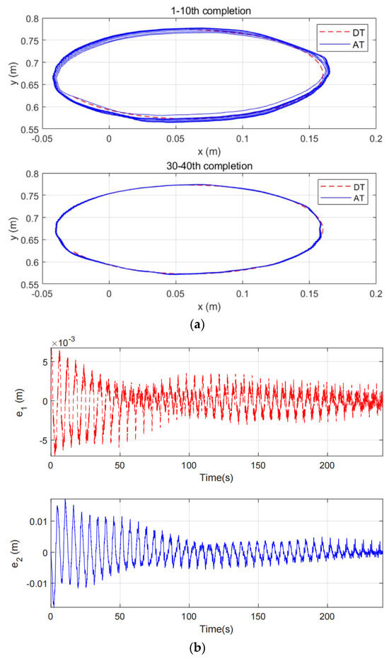
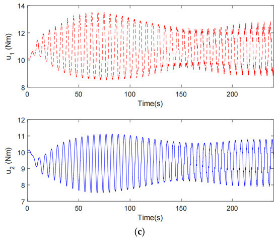
Figure 6.
The experimental results by the proposed HAC. (a) The tracking performance, (b) The tracking error, (c) The control input.
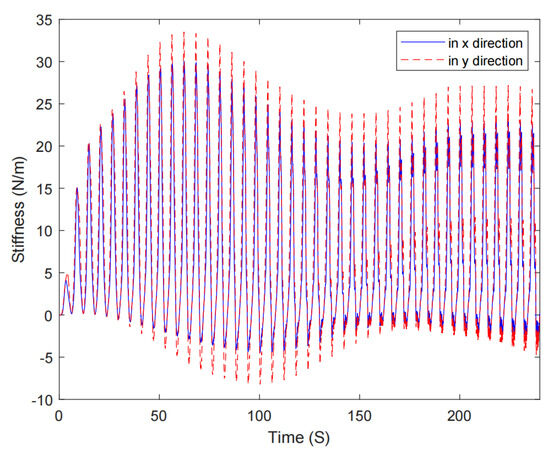
Figure 7.
The estimated stiffness by the proposed HAC.
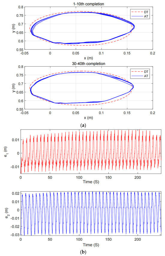
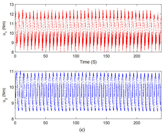
Figure 8.
The experimental results by the AC in [29]. (a) The tracking performance, (b) The tracking error, (c) The control input.
6. Conclusions
This paper presents an impedance learning-based HAC strategy for HRI with robotic modeling parameter uncertainties and human impedance uncertainties. The robotic parameter vector is constant and is estimated by a differential adaptive law with projection modification, while the time-varying impedance profile including the feedforward force, the stiffness, and the damping is estimated by periodic adaptations in (21)–(23). In Theorem 1, we prove the convergence of tracking errors and the boundedness of estimation errors using Babalat’s Lemma. Though the illustrative example on a parallel robot, we validate the following: (i) the HAC achieves time-varying impedance regulation for HRI with a stability guarantee; (ii) the asymptotic convergence of the tracking error is achieved by the HAC as opposed to the uniformly ultimately bounded results of the tracking errors in [25]; and (iii) the periodic adaptations have better performances in the estimation of time-varying impedance profiles than the differential adaptation in [25] by using the periodicity.
The subjects in this study are healthy individuals. Next, we will apply the device to patients with spasticity in upper limbs for assisted rehabilitation to study its robustness, as well as its capability in assistive movement with low tracking error in the presence of spasticity.
Author Contributions
Conceptualization, Z.J., Q.L. and J.Y.; Investigation, Z.W.; Methodology, J.Y.; Writing—original draft, Z.W.; Writing—review and editing, Z.J. and J.Y. All authors have read and agreed to the published version of the manuscript.
Funding
This research was funded by National Natural Science Foundation of China, grant number 62103280.
Data Availability Statement
The datasets used and/or analyzed during the current study are available from the corresponding author on reasonable request.
Conflicts of Interest
Author Qipeng Lv was employed by the company The Second Research Institute of China Electronics Technology Group Corporation. The remaining authors declare that the research was conducted in the absence of any commercial or financial relationships that could be construed as a potential conflict of interest.
References
- Zhang, F.; Hou, Z.G.; Cheng, L.; Wang, W.; Chen, Y.; Hu, J.; Peng, L.; Wang, H.B. iLeg—A lower limb rehabilitation robot: A proof of concept. IEEE Trans. Hum.-Mach. Syst. 2016, 46, 761–768. [Google Scholar] [CrossRef]
- Hogan, N. Impedance control: An approach to manipulation: Part II—Implementation. J. Dyn. Syst. Meas. Control 1985, 107, 8–16. [Google Scholar] [CrossRef]
- Spong, M.W.; Hutchinson, S.; Vidyasagar, M. Robot Modeling and Control, 2nd ed.; John Wiley & Sons: New York, NY, USA, 2006; pp. 1–18. [Google Scholar]
- He, W.; Tang, X.; Wang, T.; Liu, Z. Trajectory tracking control for a three-dimensional flexible wing. IEEE Trans. Contr. Syst. Technol. 2022, 30, 2243–2250. [Google Scholar] [CrossRef]
- Chan, S.P.; Yao, B.; Gao, W.B.; Cheng, M. Robust impedance control of robot manipulators. Int. J. Robot. Autom. 1991, 6, 220–227. [Google Scholar]
- Li, Z.; Huang, Z.; He, W.; Su, C.Y. Adaptive impedance control for an upper-limb robotic exoskeleton using biological signals. IEEE Trans. Ind. Electron. 2017, 64, 1664–1674. [Google Scholar] [CrossRef]
- Sun, T.; Peng, L.; Cheng, L.; Hou, Z.G.; Pan, Y. Composite learning enhanced robot impedance control. IEEE Trans. Neur. Net. Lear. 2010, 31, 1052–1059. [Google Scholar] [CrossRef]
- He, W.; Dong, Y.; Sun, C. Adaptive neural impedance control of a robotic manipulator with input saturation. IEEE Trans. Syst. Man Cybern. 2016, 46, 334–344. [Google Scholar] [CrossRef]
- Yang, C.; Chen, C.; He, W.; Cui, R.; Li, Z. Robot learning system based on adaptive neural control and dynamic movement primitives. IEEE Trans. Neur. Net. Lear. 2019, 30, 777–787. [Google Scholar] [CrossRef]
- Yang, C.; Peng, G.; Cheng, L.; Na, J.; Li, Z. Force sensorless admittance control for teleoperation of uncertain robot manipulator using neural networks. IEEE Trans. Syst. Man Cybern. A 2021, 51, 3282–3292. [Google Scholar] [CrossRef]
- He, W.; Xue, C.; Yu, X.; Li, Z.; Yang, C. Admittance-based controller design for physical human-robot interaction in the constrained task space. IEEE Trans. Autom. Sci. Eng. 2022, 19, 1937–1949. [Google Scholar] [CrossRef]
- Li, X.; Liu, Y.H.; Yu, H. Iterative learning impedance control for rehabilitation robots driven by series elastic actuators. Automatica 2018, 90, 1–7. [Google Scholar] [CrossRef]
- Buchli, J.; Stulp, F.; Theodorou, E.; Schaal, S. Learning variable impedance control. Int. J. Robot. Res. 2011, 30, 820–833. [Google Scholar] [CrossRef]
- Ajoudani, A.; Tsagarakis, N.; Bicchi, A. Tele-impedance: Teleoperation with impedance regulation using a body-machine interface. Int. J. Robot. Res. 2012, 31, 1642–1656. [Google Scholar] [CrossRef]
- Howard, M.; Braun, D.J.; Vijayakumar, S. Transferring humanimpedance behavior to heterogenous variable impedance actuators. IEEE Trans. Robot. 2013, 29, 847–862. [Google Scholar] [CrossRef]
- Kronander, K.; Billard, A. Learning compliant manipulation through kinesthetic and tactile human-robot interaction. IEEE Trans. Haptics 2013, 7, 367–380. [Google Scholar] [CrossRef]
- Abu-Dakka, F.J.; Saveriano, M. Variable impedance control and learning-a review. Front. Robot. AI 2020, 7, 590681. [Google Scholar] [CrossRef]
- Ficuciello, F.; Villani, L.; Siciliano, B. Variable impedance control of redundant manipulators for intuitive human-robot physical interaction. IEEE Trans. Robot. 2015, 31, 850–863. [Google Scholar] [CrossRef]
- Duan, J.; Gan, Y.; Chen, M.; Dai, X. Adaptive variable impedance control for dynamic contact force tracking in uncertain environment. Robot. Auton. Syst. 2018, 102, 54–65. [Google Scholar] [CrossRef]
- Kronander, K.; Billard, A. Stability considerations for variable impedance control. IEEE Trans. Robot. 2016, 32, 1298–1305. [Google Scholar] [CrossRef]
- Dong, Y.; Ren, B. UDE-based variable impedance control of uncertain robot systems. IEEE Trans. Syst. Man Cybern. A 2019, 49, 2487–2498. [Google Scholar] [CrossRef]
- Sun, T.; Peng, L.; Cheng, L.; Hou, Z.G.; Pan, Y. Stability-guaranteed variable impedance control of robots based on approximate dynamic inversion. IEEE Trans. Syst. Man Cybern. A 2021, 51, 4193–4200. [Google Scholar] [CrossRef]
- Modares, H.; Ranatunga, I.; Lewis, F.L.; Popa, D.O. Optimized assistive human-robot interaction using reinforcement learning. IEEE Trans. Cybern. 2016, 46, 655–667. [Google Scholar] [CrossRef]
- Peng, G.; Chen, C.P.; Yang, C. Robust admittance control of optimized robot-environment interaction using reference adaptation. IEEE Trans. Neur. Net. Learn. 2023, 34, 5804–5815. [Google Scholar] [CrossRef]
- Sadrfaridpour, B.; Wang, Y. Collaborative assembly in hybrid manufacturing cells: An integrated framework for human robot interaction. IEEE Trans. Autom. Sci. Eng. 2018, 15, 1178–1192. [Google Scholar] [CrossRef]
- Yang, C.; Ganesh, G.; Haddadin, S.; Parusel, S.; Albu-Schaeffer, A.; Burdet, E. Human-like adaptation of force and impedance in stable and unstable interactions. IEEE Trans. Robot. 2011, 27, 918–930. [Google Scholar] [CrossRef]
- Li, Y.; Ganesh, G.; Jarrassé, N.; Haddadin, S.; Albu-Schaeffer, A.; Burdet, E. Force, impedance, and trajectory learning for contact tooling and haptic identifification. IEEE Trans. Robot. 2018, 34, 1170–1182. [Google Scholar] [CrossRef]
- Sharifi, M.; Azimi, V.; Mushahwar, V.K.; Tavakoli, M. Impedance learning-based adaptive control for human-robot interaction. IEEE Trans. Contr. Syst. Technol. 2022, 30, 1345–1358. [Google Scholar] [CrossRef]
- Dixon, W.E.; Zergeroglu, E.; Dawson, D.M.; Costic, B.T. Repetitive learning control: A lyapunov-based approach. IEEE Trans. Syst. Man Cybern. B 2002, 32, 538–545. [Google Scholar] [CrossRef]
- Costic, B.T.; de Queiroz, M.S.; Dawson, D.N. A new learning control approach to the active magnetic bearing benchmark system. In Proceedings of the 2000 American Control Conference, Chicago, IL, USA, 28–30 June 2000; pp. 2639–2643. [Google Scholar]
Disclaimer/Publisher’s Note: The statements, opinions and data contained in all publications are solely those of the individual author(s) and contributor(s) and not of MDPI and/or the editor(s). MDPI and/or the editor(s) disclaim responsibility for any injury to people or property resulting from any ideas, methods, instructions or products referred to in the content. |
© 2024 by the authors. Licensee MDPI, Basel, Switzerland. This article is an open access article distributed under the terms and conditions of the Creative Commons Attribution (CC BY) license (https://creativecommons.org/licenses/by/4.0/).