Cartesian Stiffness Shaping of Compliant Robots—Incremental Learning and Optimization Based on Sequential Quadratic Programming

Abstract

Emerging robotic systems with compliant characteristics, incorporating nonrigid links and/or elastic actuators, are opening new applications with advanced safety features, as well as improved performance and energy efficiency in contact tasks. However, the complexity of such systems poses challenges in modeling and control due to their nonlinear nature and model variations over time. To address these challenges, the paper introduces Locally Weighted Projection Regression (LWPR) and its online learning capabilities to keep the model of compliant actuators accurate and enable the model-based controls to be more robust. The approach is experimentally validated in Cartesian position and stiffness control for a 4 DoF planar robot driven by Variable Stiffness Actuators (VSA), whose real-time implementation is supported by the Sequential Least Squares Programming (SLSQP) optimization approach.

1. Introduction

Compliant robots constitute a paradigm shift in the field of robotics, characterized by the deliberate integration of pliable materials designed to emulate the inherent flexibility and adaptability observed in natural organisms. Unlike their rigid counterparts, even ones with active compliant control strategies, compliant robots have the unique capability to undergo deformation and reconfiguration, allowing them to adapt and conform to their environment. The compliant nature of these robots imparts a level of dexterity and versatility, making them well suited for tasks that require interaction with delicate objects or for navigating complex, dynamic environments. As the field continues to advance, compliant robots have the potential to revolutionize various industries by providing innovative solutions to problems that were once deemed impossible for traditional robotic systems.

Compliant robots have an elastic element between the actuator and the link, which enables diverse variants of compliant actuators to be systematically designed and engineered by varying actuator configurations and associated elastic elements. They are capable of absorbing sudden impacts and adapting to them [1,2,3]. Furthermore, robots with flexible joints can outperform rigid robots in repetitive tasks [4], or where a high energy impact is needed to perform tasks such as throwing or nailing [5,6].

The two main types of compliant actuators that have been developed are actuators with constant or variable compliance. Constant compliance actuators or Series Elastic Actuators (SEA) have one elastic element in series to the motor shaft. To accurately control this type of actuator, the characteristics of elastic elements need to be known. The precise joint stiffness of SEA can be acquired either via Finite Element Method analysis or experimentally [7]. SEA exhibits some low-pass filter properties [8] and improves force accuracy by turning the force control problem into a position control problem [9]. However, in some tasks, constant compliance does not lead to the desired behavior—therefore, higher-precision path following might not be possible. Conversely, VSAs have a mechanical structure capable of changing the stiffness properties of the actuator. These types of actuators are mainly composed of two motors coupled with elastic springs—a bidirectional antagonistic setup [10], or they use one motor for position change and another for stiffness variation (independent motor setup) [9]. Basic VSA control methods have generally been founded upon the actuator model: feedback linearization, decoupled control, cascade control, adaptive control, etc. [11,12,13,14,15]. All these methods deal with a nonlinear model or its approximation. Generating the correct representation of the dynamical model is not a trivial task. The characteristics of the springs, as a source of compliance in compliant actuators, are often nonsymmetrical, and the geometry of the actuator itself cannot always be represented correctly. Furthermore, compliant elements are often susceptible to degradation with wear and time, which reduces model accuracy further.

Modeling motor or actuator transfer functions based on the characteristics provided by the manufacturer can be a very challenging task. Moreover, two motors from the same batch with the same declared characteristics do not have exactly matching transfer functions. Furthermore, VSAs have two motors that both work to shape the actuator characteristics, making them even more demanding to model. Consequently, the actuator model needs to be exploited from raw data. Initial approaches to learning models were based on applying step excitation and measuring actuator response. With that information, ARX, ARMAX, or other algorithms can be implemented for transfer function learning. Developing more sophisticated algorithms like neural networks, machine learning techniques, and iterative learning provides easier ways for model learning of actuators [16,17,18,19].

Many researchers in the past have implemented different learning techniques to map the relation between system inputs and outputs, tune the dynamics, or control the parameters of a system. In [20], feed-forward control was designed in the form of a PI controller, which gains updates via iterative learning. Iterative learning control was used in [21] for feed-forward control in a decentralized manner, where the feedback control part has a low-gain structure. Generalized iterative learning control for VSA trajectory tracking is presented in [22]. Furthermore, iterative learning was deployed to balance feed-forward and feedback elements described in [23], showing better results than conventional feedback control. Some papers depict a neural network-based adaptive control strategy designed for controlling VSAs [24,25]. Additionally, neural networks can be applied to predict human motion, in order to create the desired robot motion and control the robot in physical human–robot interaction [26]. Reinforcement learning is used for goal-oriented tasks and model-free control. In [27], the authors report accomplishing variable impedance control with reinforcement learning algorithms that are model-free. Furthermore, a model-based policy learning algorithm for closed-loop predictive control of soft robots was implemented in [28], where feed-forward dynamics are represented by a neural network.

The present research considered bidirectional antagonistic actuators. This type of actuator has two DC motors linked to an output shaft with springs. The output position and the stiffness of the actuator can be controlled by changing the position of the two motors. To construct the required system model, the nonlinear relation between inputs (DC motor positions) and outputs (joint position and stiffness) needs to be presented. The complexity of the model depends on the spring’s characteristics. The mathematical model almost always assumes that the system is symmetric. Since there are no two identical DC motors or two identical springs, learning algorithms can be applied to learn the model of a system. Constructing accurate models and executing control over compliant robotic systems encounter complexities due to unmodeled friction, asymmetry in springs and motors, and spring nonlinearity.

A key feature of novel compliant robots is advanced and safer physical interaction with the environment. The performance and capabilities of a robot in physical interaction are defined by the mechanical impedance of its End Effector (EE) in Cartesian space or simply by its static component—mechanical stiffness. This property is described by the Cartesian stiffness matrix—${\mathit{K}}_c$. Variations in stiffness components can be a tradeoff between the accuracy of rigid robots and the safety of compliant robots in different directions. The Cartesian stiffness matrix depends on the configuration of the robot ($\mathit{q}$) and the stiffness of each joint, which formulated the diagonal joint stiffness matrix (${\mathit{K}}_j$), see Equation (10). Therefore, accurate and fast information on the position and stiffness of compliant actuators is essential for planning and controlling the physical interaction of compliant robots that rely on models.

When it comes to the control of robots driven by rigid joints, Cartesian stiffness is mainly determined by the robot’s posture. The stiffness of classical industrial robots with rigid joints is affected by their geometry, material characteristics, actuator and transmission properties, and the robots’ posture. In order to control the Cartesian stiffness of an industrial robot and thus make it compliant, researchers have developed different control strategies like impedance and admittance control [29,30,31]. In addition, it is possible to control Cartesian stiffness if the robot has more degrees of freedom than the task space via reconfiguration in the null space [32,33,34,35,36].

However, robots with VSAs can control Cartesian stiffness via robot reconfiguration or null space variation, as well as by changing the stiffness on the joint level [37]. Using standard Cartesian stiffness-shaping techniques (active compliance, optimization algorithms), combined with robots that have flexible joints, can provide better control and a wider range of achievable Cartesian stiffness [38].

The above-mentioned collaborative approaches enhance efficiency and flexibility in production processes, reducing the risk of injury by absorbing external forces, which showcase real-world applications where compliant robots excel in industrial settings. Robots with compliant features are employed on assembly lines where they can work safely alongside human workers in the automotive industry [39,40]. Some authors propose the use of impedance control for collaborative human–robot chamfering and polishing applications [41], as well as a null-space search for torque-effective drilling [42]. Collaborative assembly via robot behavior shaping with active and passive compliance was introduced in [43]. Furthermore, a notable real-world application where compliant robots outperform rigid robots is in surgery, specifically in minimally invasive procedures. Compliant robotic systems, such as the da Vinci Surgical System [44], demonstrate superiority over rigid counterparts due to their ability to navigate and manipulate soft and delicate tissues with greater precision and dexterity [45]. The compliance of the robotic arms allows for more natural and adaptive movements, reducing the risk of tissue damage and improving surgeon’s control [46].

The contribution of this paper is twofold. The LWPR learning algorithm [47] substitutes the traditional way of modeling actuators and maps VSA characteristics, including the possibility to examine nonlinear phenomena which are often considered as unmodeled dynamics (frictions or drive asymmetry). Additionally, incremental learning features of the LWPR algorithm were used to track model parameter changes due to wear and tear. New measurements are used to expand the learning dataset and incrementally update the actuator model. The proposed methodology improves simultaneous control of both the position and passive stiffness of VSAs. Secondly, SLSQP [48,49,50,51] optimization was implemented to shape the Cartesian stiffness of compliant robots with VSAs. This algorithm exploits all the features of quadratic programming, which is used when fast optimization with constraints is needed. Furthermore, SLSQP can optimize functions that have nonlinear criteria with nonlinear constraints. The proposed methodology enables Cartesian stiffness shaping on the EE level to meet the desired robot behavior without concerning stability issues by leveraging compliant behavior via passive stiffness and robot reconfiguration in the null space. Correspondingly, combining joint-level stiffness control and reconfiguration extends the achievable Cartesian stiffness range.

To exploit the full potential of the proposed methodology, the following pipeline was defined through several steps: (1) learning VSA model parameters using LWPR; (2) continuous parameters relearning via incremental learning; (3) utilization of the learned robotic system model (in our case, 4 DoF planar robot with VSAs); and (4) SLSQP algorithm to effectively control behavior by determining the optimal configuration and stiffness on the joint level. The flow chart of the proposed pipeline is presented in Figure 1.

The rest of the paper is organized as follows. Section 2 introduces a general method of LWPR utilization for learning the model of compliant joints and then presents its use case on the QB actuator—the bidirectional antagonistic drive. Section 3 describes a general SLSQP optimization method for Cartesian stiffness shaping, as well as a use case on computing positions and stiffnesses for each of the 4 DoF compliant robot joints for the desired Cartesian stiffness. Finally, Section 4 validates the theory and use cases from Section 2 and Section 3 by introducing external disturbances via a compliant robot equipped with an F/T sensor that exposes the motion to the 4 DoF complaint robot and measures the deviation from the desired position. The paper ends with concluding remarks and future work prospects.

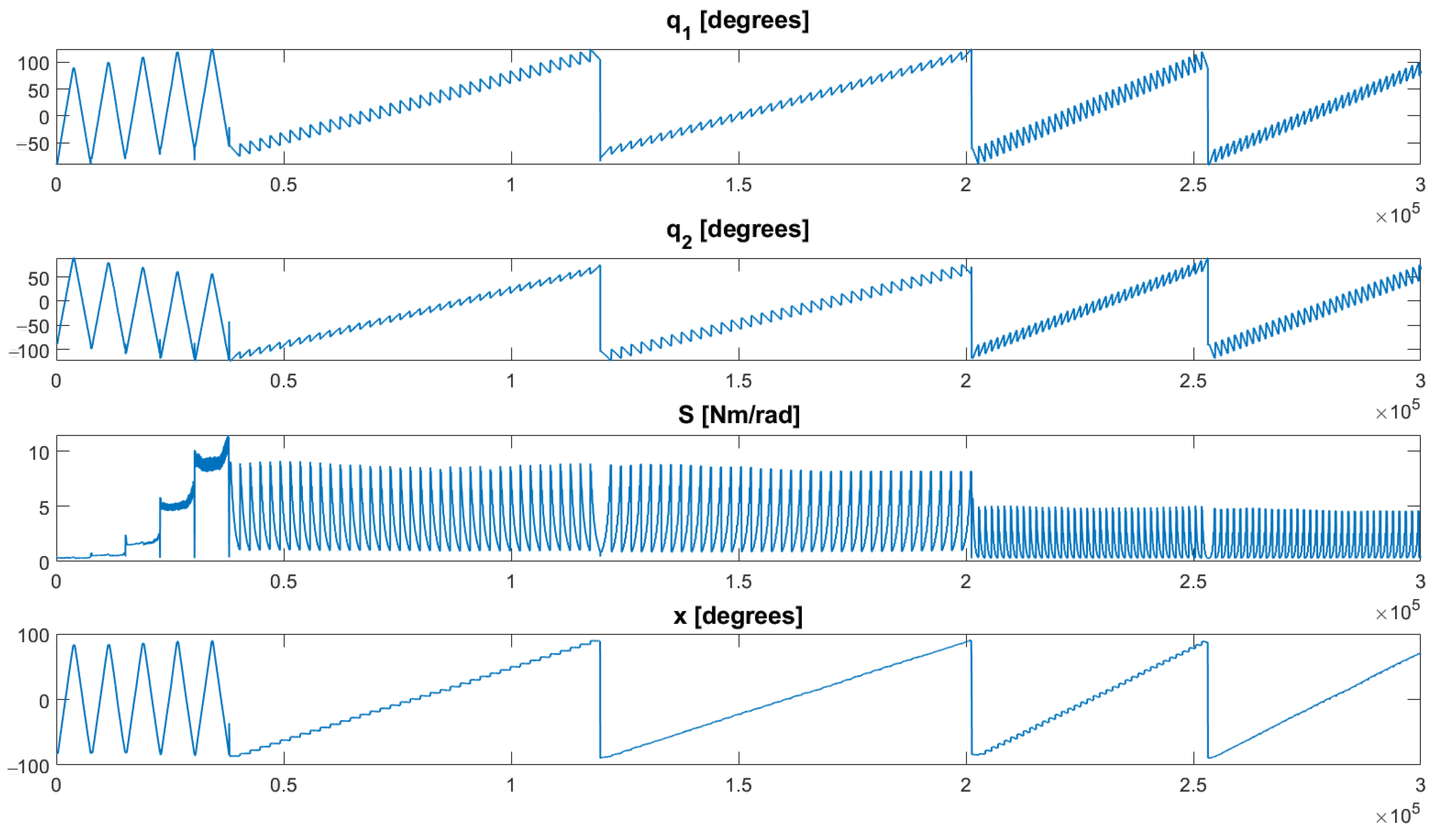
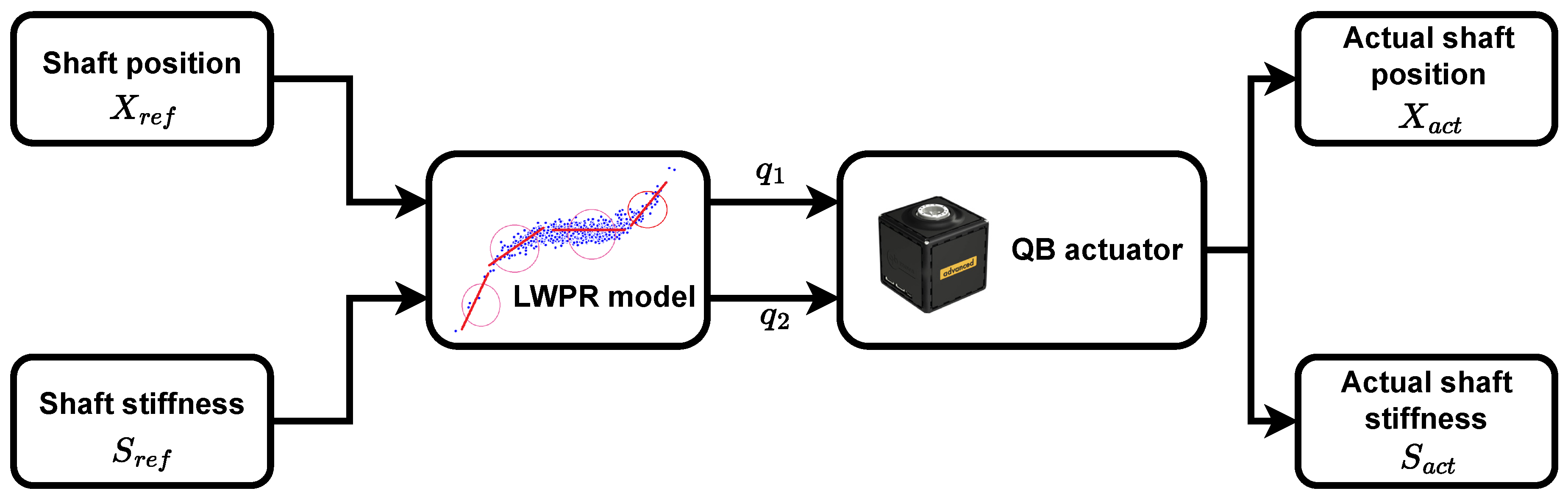
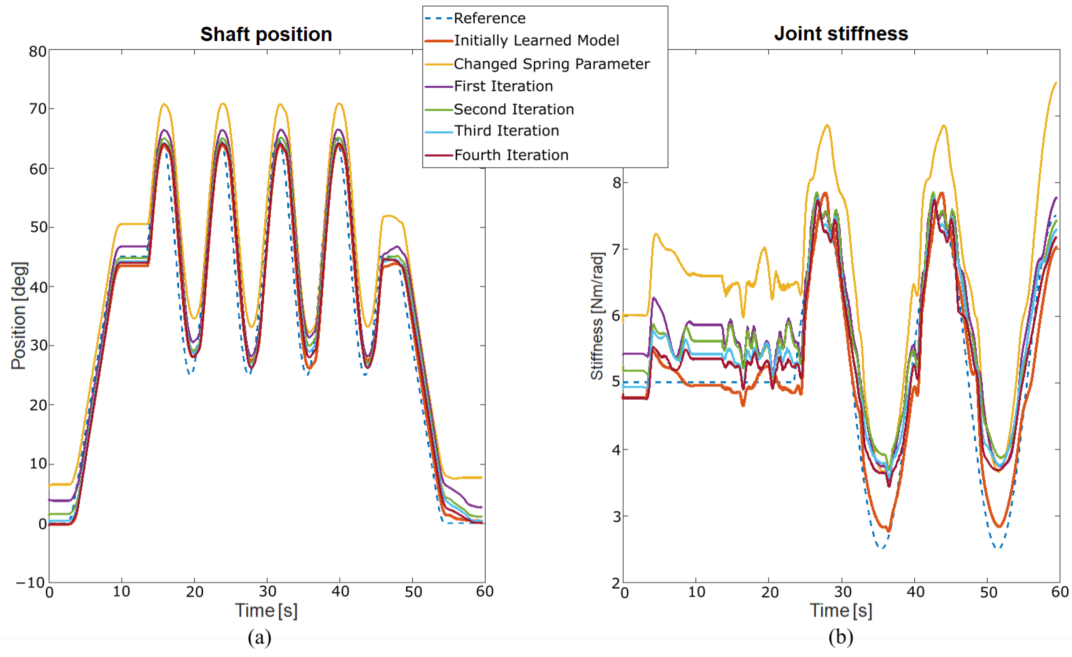
2. Learning a Variable Stiffness Actuator Model

LWPR is used as a learning technique in order to deal with the uncertainties of the actuator model parameters, as well as the nonlinearity of the actuator and its susceptibility to change due to wear. The LWPR method is designed to overcome the issue of sparse data because it is effective in learning when a small amount of data is available or when the data are noisy. In [47], the authors describe in detail the features of LWPR compared to other state-of-the-art algorithms, like the Gaussian Process and Support Vector Machine. Furthermore, the complexity of the LWPR algorithm increases linearly with problem dimensionality. Regarding computational efficiency, a $70\mathrm{Hz}$ learning rate has been achieved for a high-dimensional learning problem (90 inputs and 30 outputs). In [52], this technique is used to map the input/output characteristics of SEA. Paper [53] presents a learning algorithm to acquire the inverse dynamics of a 7 DoF manipulator. In the present paper, the LWPR algorithm is used to map the input/output characteristics of VSA, enabling nonlinear function mapping in high-dimensional space, which is very suitable for learning the behavior of robotic systems. Its main idea is to fit a nonlinear function using local linear models. It is shown that locally linear models can be an appropriate substitute for nonlinear and complex models. The essence of LWPR is to determine the validity region of each local model. The validity region can be represented in the form of a Gaussian kernel

$${\omega }_k=\exp (-\frac{1}{2}{(\mathit{x}-{\mathit{c}}_k)}^T{\mathit{D}}_k(\mathit{x}-{\mathit{c}}_k))$$

(1)

where ${\mathit{c}}_k$ is the center of kth linear model, and ${\mathit{D}}_k$ corresponds to a positive semi-definite distance metric that determines the size and shape of the validity region of the linear model. Algorithms update the distance matrix ${\mathit{D}}_k({\mathit{D}}_k={\mathit{M}}_k^T{\mathit{M}}_k)$ by incorporating gradient descent

$${\mathit{M}}_k^{n+1}={\mathit{M}}_k^n-\alpha \frac{𝜕J}{𝜕{\mathit{M}}_{\mathit{k}}},$$

(2)

where J is the criteria function for minimizing the prediction error of all linear models.

For each input query data, the local linear model calculates the prediction ${\widehat{y}}_k$. The total output of the learning system is the normalized weighted mean of all K linear models

$$\widehat{y}=\sum _1^K{\omega }_k{\widehat{y}}_k/\sum _1^K{\omega }_k.$$

(3)

To successfully incorporate the LWPR approach into a learning problem, the learning rate parameter $\alpha$ and the initial values for the distance matrix ${\mathit{D}}_k$ need to be set properly. The typical approach, which can be applied to various VSAs, involves configuring the parameter ${\mathit{D}}_k=r\mathit{I}$ with a small number for the variable r (e.g., $r=0.05$). Then, the model is retrained by gradually increasing r until the model achieves satisfactory performance. Also, $\alpha$ can be tuned to improve algorithm performance. This methodology might be demanding and time-consuming until satisfactory performance is achieved.

QB Move Maker Pro [54] was used in this research as a bidirectional antagonistic actuator. Figure 2 shows the QB actuator and its functional scheme. This actuator is a low-cost and open-source variable stiffness actuator. It can be represented as a system with two inputs ($q_1$ and $q_2$) and two outputs (x and S), where $q_1$ and $q_2$ are the positions of the primal mover motors (DC motors), and x and S are the output shaft position and joint stiffness, respectively. The static relation between the position of the QB actuator primal movers and the equilibrium position and stiffness is given by Equations (4) and (5)

$$x_e=(q_1+q_2)/2,$$

(4)

$$S_e=a·k·\mathrm{c}osh(a·(x-q_1))+a·k·\mathrm{c}osh(a·(x-q_2)).$$

(5)

Here, $\mathrm{c}osh$ is the cosine hyperbolic function, while $a=6.8465$ and $k=0.0223$ are spring parameters obtained via identification.

A proper training set needs to be collected to map the static relation between the inputs and outputs of the bidirectional antagonistic actuator. In the proposed application case, a 4 DoF planar manipulator with VSAs, the input dimension is $2\times 4$ (shaft position and joint stiffness of each actuator), and the output dimension is also $2\times 4$ (primal movers position of each actuator). Data collection is performed on a QB actuator. The authors of [55] suggest five different patterns of the input/output signals). In the first pattern, the reference signals for the primal movers are assumed to have a constant difference between them (0, 20, 40, 60, and ${70}^{°}$), achieving constant stiffness in each subpattern. The difference between the primal movers keeps the constant position of each primal mover from changing from $-90$ to 90 by $5^{°}$. In the following four patterns, the position of the primal movers changed increasingly from $-90$ to ${90}^{°}$ and the difference between their positions changed up and down from $-60$ to ${60}^{°}$. The dataset is presented in Figure 3.

After designing and collecting the training data, the actuator model was learned and the feed-forward control method was implemented. Feed-forward control was used to faithfully represent the accuracy of the learned model. The following diagram represents the control functional scheme (Figure 4).

The results from the learned model and the mathematical representation of the static actuator model are shown in Figure 5, to illustrate how well this model can track reference motion. The static model was formed using Equations (4) and (5).

It is apparent in Figure 5 that the LWPR and static models of the actuator yield similar position tracking results, but the LWPR model is better in stiffness tracking. However, more effort needs to be put into conducting the detailed mathematical model (including spring and motor asymmetries and friction) compared to the LWPR method, since machine learning techniques simplify model development.

To represent the incremental learning features of the LWPR algorithm, a series of experiments were performed in a simulation environment, using the same learning methodology. After data collection, learning of the actuator model proceeded with LWPR. The initial results from the feed-forward control are shown in Figure 6, light red). Changing the characteristics of one spring on this simulated actuator led to undesired behavior. It is obvious that with new spring parameters, the previously learned model did not consistently track the reference path and stiffness. The reason for this is evident since the actuator model was learned for the initial model parameters (Figure 6, yellow).

When the classical mathematical model is used, a robust controller needs to be developed to suppress the disturbance due to the change in actuator parameters. Designing a robust controller for this type of highly nonlinear system can be challenging. Consequently, it is more convenient to use the incremental learning features of the LWPR. The same model that was learned at the beginning can be used in the process of relearning. Due to model uncertainties introduced by drastic parameter changes (not likely to happen in real-life scenarios, where parameter degradation occurs gradually), new measurements are introduced in the learning set. The new actuator model was learned successfully after only four iterations (Figure 6). In the case of a large deviation from the initial parameters, the model can be relearned an arbitrary number of times.

3. Planning End-Effector Cartesian Stiffness

This section presents an optimization algorithm for shaping a robot’s EE Cartesian stiffness. To achieve the desired stiffness, the nonlinear function needed to be minimized. SLSQP optimization was used to shape the Cartesian stiffness. This method is an iterative procedure for minimizing nonlinear functions with nonlinear constraints. In each iteration, SLSQP was reduced to a quadratic programming (QP) subproblem by transforming nonlinear functions into quadratic approximation. Furthermore, the result of one QP iteration was used as the starting point for another SLSQP iteration. The problem statement can be formulated as follows

$$\begin{array}{c}\hfill \begin{array}{c}\hfill minf\left(\mathit{\omega }\right),\mathrm{over}\mathit{\omega }\in {\mathbb{R}}^n,\\ \hfill \mathrm{subject}\mathrm{to}h\left(\mathit{\omega }\right)=0,\\ \hfill g\left(\mathit{\omega }\right)\le 0,\end{array}\end{array}$$

(6)

where the objective function is represented as $f:{\mathbb{R}}^n\to \mathbb{R}$, while functions $h:{\mathbb{R}}^n\to {\mathbb{R}}^m$ and $g:{\mathbb{R}}^n\to {\mathbb{R}}^z$ are the equality and inequality constraints for an optimization problem. The value n represents the number of variables in vector $\mathit{\omega }$ (robot’s joints position vector and joint stiffnesses) for which optimization is performed, and m and z are the number of equality or inequality constraints, respectively.

For redundant compliant robots, there is an infinite number of robot configurations for one EE position. EE Cartesian stiffness can be alternated by changing the configuration and joint stiffness of the robot. The primary focus of the authors’ previous research was the EE Cartesian stiffness control of task-redundant robots with SEAs [56]. The SLSQP algorithm was used to optimize the robot configuration via the null space search, in order to achieve the desired EE Cartesian stiffness. This paper provides an extension of the topic by introducing VSAs in the 4 DoF planar manipulator. To run the optimization algorithm, a kinematic model of the proposed robotic system needed to be developed.

Based on Figure 7, the Cartesian position of the robot EE is defined as

$$x=l_1\cos \left(q_1\right)+l_2\cos (q_1+q_2)+l_3\cos (q_1+q_2+q_3)+l_4\cos (q_1+q_2+q_3+q_4),$$

(7)

$$y=l_1\sin \left(q_1\right)+l_2\sin (q_1+q_2)+l_3\sin (q_1+q_2+q_3)+l_4\sin (q_1+q_2+q_3+q_4),$$

(8)

$$\theta =q_1+q_2+q_3+q_4,$$

(9)

where $q_1$, $q_2$, $q_3$, $q_4$ are the joint positions and $l_1$, $l_2$, $l_3$, $l_4$ are the lengths of the robot links. The robot stiffness in the Cartesian space is in direct relation to the robot configuration and, therefore, directly related to the Jacobian matrix $\mathit{J}$.

In the case of VSA-driven robots, Cartesian stiffness is influenced by the robot joint stiffness matrix that has a diagonal matrix form ${\mathit{K}}_j=\mathrm{diag}\left(k_i\right)$, where $k_i$ is the i-th joint stiffness. The Cartesian stiffness matrix can be defined as

$${\mathit{K}}_c={\left(\mathit{J}\left(\mathit{q}\right){\mathit{K}}_j^{-1}\mathit{J}{\left(\mathit{q}\right)}^T\right)}^{-1},$$

(10)

where ${\mathit{K}}_c$ is the symmetric $2\times 2$ matrix and $\mathit{q}$ is a 4-dimensional joint position vector.

Only optimization of the $k_{c_{11}}$ and $k_{c_{22}}$ elements will be considered, as they represent stiffness along the X and Y axes in Cartesian coordinates

$${\mathit{K}}_{co}=\left[\begin{array}{cc}{k}_{c_{11}}& 0\\ 0& k_{c_{22}}\end{array}\right],$$

(11)

where $k_{c_{11}}$ is stiffness along the X axis and $k_{c_{22}}$ is stiffness along the Y axis. The desired Cartesian stiffness can be represented as a $2\times 2$ diagonal matrix

$${\mathit{K}}_{cd}=\left[\begin{array}{cc}{k}_{c{d}_x}& 0\\ 0& k_{c{d}_y}\end{array}\right].$$

(12)

For the purpose of optimization, the weighted Frobenius norm was used to describe the process performance index (criteria function). The task was to minimize the norm $f\left(\mathit{\omega }\right)$ and therefore achieve stiffness tracking.

$$f\left(\mathit{\omega }\right)=\sqrt{A{(k_{c{d}_x}-k_{c_{11}})}^2+B{(k_{c{d}_y}-k_{c_{22}})}^2}.$$

(13)

Coefficients A and B are weighted factors used to favor one axis over the other. For the optimization process, following the desired EE position can be considered as an optimization constraint. In fact, the optimization process needs to find the robot joint coordinates $q_{o1}$, $q_{o2}$, $q_{o3}$, $q_{o4}$ and joint stiffness $k_{j_{o1}}$, $k_{j_{o2}}$, $k_{j_{o3}}$, $k_{j_{o4}}$ that provides the minimal norm (Equation (13)) and satisfies the constraint that can be described by

$$h{\left(\mathit{\omega }\right)}_1=-x_d+l_1\cos \left(q_{o1}\right)+l_2\cos (q_{o1}+q_{o2})+l_3\cos (q_{o1}+q_{o2}+q_{o3})+l_4\cos (q_{o1}+q_{o2}+q_{o3}+q_{o4}),$$

(14)

$$h{\left(\mathit{\omega }\right)}_2=-y_d+l_1\sin \left(q_{o1}\right)+l_2\sin (q_{o1}+q_{o2})+l_3\sin (q_{o1}+q_{o2}+q_{o3})+l_4\sin (q_{o1}+q_{o2}+q_{o3}+q_{o4}).$$

(15)

By repeating this process, the optimization algorithm can lead to a local minimum because the algorithm is based on gradient descent.

A simulated 4 DoF planar manipulator was used to validate the optimization technique. In the simulation, the robot link lengths were set at $l_1=l_2=l_3=l_4=0.1\mathrm{m}$. First, the optimization process was simulated over one axis, then over the X axis and Y axis simultaneously. To prove that the optimization technique was working, several cases of the desired robot configuration and stiffness were introduced in the simulation. QB Move Maker Pro parameters were used to achieve more realistic simulation results. The active rotation angle was $\pm {180}^{°}$, and the minimal and maximal stiffness were $0.5\mathrm{Nm}/\mathrm{rad}$ and $13\mathrm{Nm}/\mathrm{rad}$, respectively. At the beginning of each simulation, the initial robot joint stiffness was set to $5\mathrm{Nm}/\mathrm{rad}$. The time needed to calculate the optimal robot configuration and joint stiffnesses was $0.004\pm 0.001\mathrm{s}$.

3.1. Optimization over One Axis

For one-axis optimization, the value of one coefficient, A or B, in Equation (13) needed to be set to 0. If coefficient A is 0, then optimization is performed over the Y axis and vice versa. The robot manipulator is set at some point in the workspace and the algorithm is started. A couple of trials of one-axis optimization are presented in

Table 1. One-axis optimization across Y axis.

Sim.	Desired Pos.	Init. Conf.	Res. Stiff.	Res. Conf.	Res. Pos.	Norm Val.	Stiffness:
	$\mathit{x},\mathit{y}$	${\mathit{q}}_{\mathbf{1},\mathbf{2},\mathbf{3},\mathbf{4}}$	${\mathit{k}}_{{\mathit{j}}_{\mathbf{1},\mathbf{2},\mathbf{3},\mathbf{4}}}$	${\mathit{q}}_{\mathbf{1},\mathbf{2},\mathbf{3},\mathbf{4}}$	$\mathit{x},\mathit{y}$		Ach. (Des.)
	[m]	[Rad]	[Nm/Rad]	[Rad]	[m]		[N/m]
1	0.0241	1.1472	7.1004	1.5707	0.0241	$2.8055\times {10}^{-5}$	235
		1.1272	0.5348	−0.8605
	0.3564	−0.2472	3.5427	0.9859	0.3564		(235)
		0.7154	0.6301	0.2777
2	0.0241	0.9472	6.7482	1.2941	0.0241	$6.6554\times {10}^{-6}$	440
		0.8972	1.6680	−0.2958
	0.3564	−0.2472	4.5738	0.5010	0.3564		(440)
		0.9054	2.5607	0.7727
3	0.1125	1.1472	2.0157	0.8516	0.1125	$6.0982\times {10}^{-5}$	728.08
		1.1272	0.5133	0.0298
	0.3198	0.0146	12.0378	1.3616	0.3198		(745)
		−0.8554	3.7201	−1.1421
4	0.1125	0.9472	5.9942	0.9342	0.1125	$1.1922\times {10}^{-5}$	1350
		0.8972	2.7714	−0.2770
	0.3198	0.0146	9.3229	1.5074	0.3198		(1350)
		−0.0783	3.1778	−0.8967

.

Robot joint stiffness was changed during the simulation, as was joint position, in order to achieve the desired stiffness at a particular position in the workspace. As shown in Table 1, in the case of the one-axis optimization, the algorithm is capable of finding a robot configuration that satisfies the constraints and achieves the desired stiffness along the selected axis.

3.2. Multiple Axis Optimization

Optimization over multiple axes was expected to be more complicated than over one axis, leading to deviation from the desired Cartesian stiffness tracking. In general, the algorithm needs to satisfy the constraints first and then find the robot configuration and joint stiffness that will achieve the desired Cartesian stiffness along multiple axes. To obtain results, coefficients A and B were set at value 1. Even though the optimization algorithm found the optimal robot configuration and joint stiffness that successfully tracked the desired Cartesian stiffness, as shown in

Table 2. Multiple axes optimization.

Sim.	Desired Pos.	Init. Conf.	Res. Stiff.	Res. Conf.	Res. Pos.	Norm Val.	Stiffness:
	$\mathit{x},\mathit{y}$	${\mathit{q}}_{\mathbf{1},\mathbf{2},\mathbf{3},\mathbf{4}}$	$\mathit{x},\mathit{y}$	${\mathit{q}}_{\mathbf{1},\mathbf{2},\mathbf{3},\mathbf{4}}$	$\mathit{x},\mathit{y}$		Ach. (Des.)
	[m]	[Rad]	[Nm/Rad]	[Rad]	[m]		[N/m]
1	0.0241	1.1472	12.9489	0.9865	0.0241	$1.6819\times {10}^{-4}$	60; 350
		1.1272	13	0.1284
	0.3564	−0.2472	3.4717	0.7027	0.3564		(60; 350)
		0.7154	0.5000	0.2841
2	0.0241	0.9472	12.6546	1.5690	0.0241	$9.0114\times {10}^{-4}$	75; 2700
		0.8972	12.7370	0.3654
	0.3564	−0.2472	8.5553	−1.2348	0.3564		(75; 2700)
		0.9054	5.0958	1.0421
3	0.1125	1.1472	7.1619	1.4837	0.1125	$1.4\times {10}^{-3}$	149.9; 499.9
		1.1272	5.9281	0.4001
	0.3198	0.0146	8.3310	−0.7289	0.3198		(150; 500)
		−0.8554	5.5392	−0.8127
4	0.2125	0.3224	12.4952	1.4081	0.2125	$1.2870\times {10}^{-4}$	500; 200
		0.0336	3.5669	0.1878
	0.2198	0.3768	8.0491	−1.5175	0.2198		(500; 200)
		1.3664	12.3320	0.0554

, the optimization algorithm can fail to find a solution that could track the desired stiffness. Two main reasons can lead to this behavior: (1) in a particular position, the robot cannot physically achieve the desired stiffness, or (2) the optimization algorithm is stuck at the local minimum. This can be overcome by multiple trials of the same desired position and stiffness with different initial positions to find the global minimum. In some scenarios, ideal Cartesian stiffness tracking is not mandatory since in most cases, it is satisfactory to achieve stiff or compliant behavior in a moving direction.

3.3. Favoring One of the Axes

In the process of multi-axes optimization, in order to favor one axis over another, coefficients A and B need to be set accordingly. To favor stiffness tracking along the X axis, the relation $A>B$ needs to be satisfied and vice versa. This case is different from simple one-axis optimization (where the user has no control over the second axis at all), because control over the non-favored axis is achieved as well.

Table 3. Favoring one of the axes.

Sim.	Desired Pos.	A and B	Res. Stiff.	Res. Conf.	Res. Pos.	Norm Val.	Stiffness:
	$\mathit{x},\mathit{y}$		${\mathit{k}}_{{\mathit{j}}_{\mathbf{1},\mathbf{2},\mathbf{3},\mathbf{4}}}$	${\mathit{q}}_{\mathbf{1},\mathbf{2},\mathbf{3},\mathbf{4}}$	$\mathit{x},\mathit{y}$		Ach. (Des.)
	[m]		[Nm/Rad]	[Rad]	[m]		[N/m]
1	0.1172	1	13	1.5708	0.1172	$89.86$	243; 874
			0.5	−0.4909
	0.3164	1	12.99	−0.7612	0.3164		(330; 850)
			6.1066	1.5040
2	0.1172	1	13	1.5708	0.1172	170	159; 847
			7.6633	−0.9172
	0.3164	16	13	0.0357	0.3164		(330; 850)
			5.4937	1.2859
3	0.1172	16	12.9728	1.5653	0.1172	$72.35$	330; 834
			5.8234	−0.2659
	0.3164	1	0.8217	−1.0942	0.3164		(330; 850)
			12.9846	1.4461

shows how changing coefficients A and B affects Cartesian stiffness tracking.

4. Experimental Validation

For experimental validation, a 4 DoF planar manipulator with QB actuators was used to demonstrate the methodology introduced for compliant actuator model learning (Section 2) and compliant robot Cartesian stiffness shaping (Section 3). To that end, the pipeline presented in Figure 1 was followed. In this process, the joint position and stiffness were obtained from the desired EE position (as a constraint) and Cartesian stiffness. Afterward, the learned LWPR models of each actuator were used to control each joint and achieve the desired joint behavior (position and stiffness). The block diagram of the whole control process is shown in Figure 8. Joint position and stiffness can be calculated from Equations (4) and (5), and the robot EE position and its Cartesian stiffness from Equations (7)–(10).

In order to estimate the achieved robot behavior, a contact or disturbance needed to be introduced to the system. This was performed with the Panda robot and the relative deviation from the equilibrium position was measured [57]. The Panda is equipped with an F/T sensor which was used to measure generated contact forces and torques. The experimental setup was composed of the 4 DoF planar robot, the Panda robot, and the F/T sensor (Figure 9), similar to that presented in [58].

A random perturbation was applied to be able to exploit the achieved behavior of the 4 DoF planar robot. The disturbance was applied in proximity to the equilibrium position. In that way, the robot configuration did not deviate from the optimal configuration, since deviation does not affect Cartesian stiffness due to the infinitesimal change in the Jacobian matrix. In the general case, the Cartesian stiffness matrix of a planar robot is given by

$${\mathit{K}}_{\mathit{C}}=\left[\begin{array}{cc}{k}_{c_{11}}& k_{c_{12}}\\ k_{c_{21}}& k_{c_{22}}\end{array}\right],$$

(16)

where $k_{c_{11}}$ and $k_{c_{22}}$ represent stiffness across the X and Y axes, respectively, and $k_{c_{12}}=k_{c_{21}}$ is the coupling stiffness between two axes.

The disturbance or contact in such a system leads to a force generated between the robot and the object in contact (Panda robot). If it is assumed that the behavior of the system is linear in proximity to equilibrium, then the generated force can be expressed as follows

$$\begin{array}{c}\hfill \mathit{F}={\mathit{K}}_{\mathit{C}}\times \Delta \mathit{X},\\ \hfill \left[\begin{array}{c}{F}_x\\ F_y\end{array}\right]=\left[\begin{array}{cc}{k}_{c_{11}}& k_{c_{12}}\\ k_{c_{21}}& k_{c_{22}}\end{array}\right]\times \left[\begin{array}{c}\Delta x\\ \Delta y\end{array}\right],\\ \hfill F_x=k_{c_{11}}\Delta x+k_{c_{12}}\Delta y\\ \hfill F_y=k_{c_{21}}\Delta x+k_{c_{22}}\Delta y.\end{array}$$

(17)

This incomplete system of equations needs to be solved in order to estimate the Cartesian stiffness matrix elements. The measured values are forces and deviation in the $XY$ plane, and the unknown variables are $k_{c_{11}}$, $k_{c_{12}}$, and $k_{c_{22}}$. If there are N randomly applied disturbances, the above equations can be rewritten as

$${\left[\begin{array}{c}{F}_{x_1}\\ F_{x_2}\\ ⋮\\ F_{x_N}\\ F_{y_1}\\ F_{y_2}\\ ⋮\\ F_{y_N}\end{array}\right]}_{2N\times 1}={\left[\begin{array}{ccc}\Delta x_1& \Delta y_1& 0\\ \Delta x_2& \Delta y_2& 0\\ ⋮& ⋮& ⋮\\ \Delta x_N& \Delta y_N& 0\\ 0& \Delta x_1& \Delta y_1\\ 0& \Delta x_2& \Delta y_2\\ ⋮& ⋮& ⋮\\ 0& \Delta x_N& \Delta y_N\end{array}\right]}_{2N\times 3}\times {\left[\begin{array}{c}{k}_{c_{11}}\\ k_{c_{12}}\\ k_{c_{22}}\end{array}\right]}_{3\times 1}$$

(18)

Using pseudoinverse, the disturbance matrix can be inverted and added to the left side of the equation, providing an estimation of unknown parameters. With this method, the Cartesian stiffness matrix parameters were fitted to minimize the Mean Least Square Error. Figure 10 represents the perturbations and the generated external forces. The applied disturbance was a random movement of the Panda robot in the $XY$ plane, where the maximal movement in each direction was $1.5\mathrm{cm}$.

The parameters of the Cartesian stiffness matrix were estimated using the previous equation. The estimated values in this experiment were

$$\widehat{{\mathit{K}}_{\mathit{c}}}=\left[\begin{array}{cc}88.6916& 21.4254\\ 21.4254& 326.0492\end{array}\right],$$

(19)

while the commanded Cartesian stiffness matrix was

$${\mathit{K}}_{\mathit{c}}=\left[\begin{array}{cc}77.0128& 0.0019\\ 0.0019& 308.1533\end{array}\right].$$

(20)

After estimating the Cartesian stiffness matrix parameters, the estimate of the generated force was calculated by using the newly estimated parameters

$$\begin{array}{c}\hfill {\widehat{F}}_x={\widehat{k}}_{c_{11}}\Delta x+{\widehat{k}}_{c_{12}}\Delta y,\\ \hfill {\widehat{F}}_y={\widehat{k}}_{c_{21}}\Delta x+{\widehat{k}}_{c_{22}}\Delta y.\end{array}$$

(21)

Plot (b) in Figure 10 (red) shows the estimated force from the applied disturbance. It is apparent from the estimated force values that using pseudoinverse to minimize the mean least square error can provide good estimation for the Cartesian stiffness parameters.

Interpretation of the Cartesian stiffness matrix can be challenging in some cases. A more convenient way of depicting the Cartesian stiffness matrix is an ellipse representation of the matrix using eigenvalue decomposition. Figure 11 shows the 4 DoF QB robot configuration, the commanded Cartesian stiffness ellipse (black), and the estimated Cartesian stiffness ellipse (red).

The estimated stiffness matrix was approximately equal to the commanded one. The error in the orientation of the estimated Cartesian stiffness ellipse was $2.8\%$ compared to the commanded Cartesian stiffness ellipse.

5. Conclusions

The research aimed to facilitate the physical interaction of a novel compliant robot with the environment by deploying the latest optimization tools and learning methods. The effort reconciled the challenges in modeling actuators of variable stiffness and the need to efficiently determine the position and stiffness of such actuators in order to plan the interaction of the robot EE with the environment. The LWPR iterative learning algorithm demonstrated its efficiency in learning the model parameters of a compliant actuator, which is prone to change due to wear and tear and exploitation time. Based on the model of the robot and its drives, SLSQP efficiently optimized the setting up of the optimal kinematic configuration of the robot and stiffness on the joint level for the desired robot EE Cartesian position and stiffness. Although the proposed methodology was experimentally validated on a 4 DoF planar robot driven by VSAs, the methodology is general and could be exploited by other compliant robots without any additional sensors. Future work will address further improvements of the proposed methodology to allow online Cartesian stiffness shaping beyond discrete points in space (e.g., along a prescribed trajectory), and consequently, its application to real-life in-contact tasks. The proposed approach has several limitations. Finding of the proper learning parameters for the LWPR algorithm can be time consuming on occasion, although parameter finding needs to be performed only once during the initial learning process. EE Cartesian stiffness is limited since it is achieved by exploiting the passive stiffness and kinematics of the manipulator. Cartesian stiffness is shaped using an optimization method that cannot guarantee a global minimum. Although time consuming, this can be overcome by calculating optimal solutions from different initial points. In future work, studies will be conducted on learning techniques that can capture motor dynamics, where a time series dataset will be used. Also, the focus will be on algorithms that combine active and passive stiffness control at the joint level to enhance the algorithm’s performance.

References

1. Peshkin, M.A.; Colgate, J.E.; Wannasuphoprasit, W.; Moore, C.A.; Gillespie, R.B.; Akella, P. Cobot architecture. IEEE Trans. Robot. Autom. 2001, 17, 377–390. [Google Scholar] [CrossRef]
2. Haddadin, S.; Albu-Schaffer, A.; De Luca, A.; Hirzinger, G. Collision Detection and Reaction: A Contribution to Safe Physical Human-Robot Interaction. In Proceedings of the 2008 IEEE/RSJ International Conference on Intelligent Robots and Systems, Nice, France, 22–26 September 2008; pp. 3356–3363. [Google Scholar] [CrossRef]
3. Bicchi, A.; Tonietti, G.; Bavaro, M.; Piccigallo, M. Variable Stiffness Actuators for Fast and Safe Motion Control. In Robotics Research. The Eleventh International Symposium; Dario, P., Chatila, R., Eds.; Springer: Berlin/Heidelberg, Germany, 2005; pp. 527–536. [Google Scholar]
4. Visser, L.C.; Stramigioli, S.; Bicchi, A. Embodying Desired Behavior in Variable Stiffness Actuators. IFAC Proc. Vol. 2011, 44, 9733–9738. [Google Scholar] [CrossRef]
5. Haddadin, S.; Weis, M.; Wolf, S.; Albu-Schäffer, A. Optimal Control for Maximizing Link Velocity of Robotic Variable Stiffness Joints. IFAC Proc. Vol. 2011, 44, 6863–6871. [Google Scholar] [CrossRef]
6. Garabini, M.; Passaglia, A.; Belo, F.; Salaris, P.; Bicchi, A. Optimality principles in variable stiffness control: The VSA hammer. In Proceedings of the 2011 IEEE/RSJ International Conference on Intelligent Robots and Systems, San Francisco, CA, USA, 25–30 September 2011; pp. 3770–3775. [Google Scholar] [CrossRef]
7. Logozzo, S.; Malvezzi, M.; Achilli, G.; Valigi, M. Characterization of finger joints with underactuated modular structure. Mater. Res. Proc. 2022, 26, 201. [Google Scholar]
8. Pratt, G.A.; Williamson, M.M. Series elastic actuators. In Proceedings of the 1995 IEEE/RSJ International Conference on Intelligent Robots and Systems. Human Robot Interaction and Cooperative Robots, Pittsburgh, PA, USA, 5–9 August 1995; Volume 1, pp. 399–406. [Google Scholar] [CrossRef]
9. Junior, A.G.L.; de Andrade, R.M.; Filho, A.B. Series Elastic Actuator: Design, Analysis and Comparison. In Recent Advances in Robotic Systems; IntechOpen: Rijeka, Croatia, 2016; Chapter 10. [Google Scholar] [CrossRef]
10. Petit, F.; Chalon, M.; Friedl, W.; Grebenstein, M.; Albu-Schäffer, A.; Hirzinger, G. Bidirectional antagonistic variable stiffness actuation: Analysis, design Implementation. In Proceedings of the 2010 IEEE International Conference on Robotics and Automation, Anchorage, AK, USA, 3–7 May 2010; pp. 4189–4196. [Google Scholar] [CrossRef]
11. Buondonno, G.; De Luca, A. Efficient Computation of Inverse Dynamics and Feedback Linearization for VSA-Based Robots. IEEE Robot. Autom. Lett. 2016, 1, 908–915. [Google Scholar] [CrossRef]
12. Trumić, M.; Jovanović, K.; Fagiolini, A. Decoupled nonlinear adaptive control of position and stiffness for pneumatic soft robots. Int. J. Robot. Res. 2021, 40, 277–295. [Google Scholar] [CrossRef]
13. Palli, G.; Melchiorri, C.; De Luca, A. On the Feedback Linearization of Robots with Variable Joint Stiffness. In Proceedings of the 2008 IEEE International Conference on Robotics and Automation, Pasadena, CA, USA, 19–23 May 2008; pp. 1753–1759. [Google Scholar] [CrossRef]
14. Potkonjak, V.; Svetozarevic, B.; Jovanovic, K.; Holland, O. The Puller-Follower Control of Compliant and Noncompliant Antagonistic Tendon Drives in Robotic Systems. Int. J. Adv. Robot. Syst. 2011, 8, 69. [Google Scholar] [CrossRef]
15. Lukić, B.; Jovanović, K.; Šekara, T.B. Cascade Control of Antagonistic VSA—An Engineering Control Approach to a Bioinspired Robot Actuator. Front. Neurorobot. 2019, 13, 69. [Google Scholar] [CrossRef]
16. Weerasooriya, S.; El-Sharkawi, M. Identification and control of a DC motor using back-propagation neural networks. IEEE Trans. Energy Convers. 1991, 6, 663–669. [Google Scholar] [CrossRef]
17. Ismeal, G.A.; Kyslan, K.; Fedák, V. DC motor identification based on Recurrent Neural Networks. In Proceedings of the 16th International Conference on Mechatronics–Mechatronika 2014, Brno, Czech Republic, 3–5 December 2014; pp. 701–705. [Google Scholar] [CrossRef]
18. Rubaai, A.; Kotaru, R. Online identification and control of a DC motor using learning adaptation of neural networks. IEEE Trans. Ind. Appl. 2000, 36, 935–942. [Google Scholar] [CrossRef]
19. Gautier, M.; Jubien, A.; Janot, A. New iterative learning identification and model based control of robots using only actual motor torque data. In Proceedings of the 2013 IEEE/ASME International Conference on Advanced Intelligent Mechatronics, Wollongong, NSW, Australia, 9–12 July 2013; pp. 1436–1441. [Google Scholar] [CrossRef]
20. Ono, S.; Masuya, K.; Takagi, K.; Tahara, K. Trajectory tracking of a one-DOF manipulator using multiple fishing line actuators by iterative learning control. In Proceedings of the 2018 IEEE International Conference on Soft Robotics (RoboSoft), Livorno, Italy, 24–28 April 2018; pp. 467–472. [Google Scholar]
21. Angelini, F.; Santina, C.D.; Garabini, M.; Bianchi, M.; Gasparri, G.M.; Grioli, G.; Catalano, M.G.; Bicchi, A. Decentralized Trajectory Tracking Control for Soft Robots Interacting With the Environment. IEEE Trans. Robot. 2018, 34, 924–935. [Google Scholar] [CrossRef]
22. Angelini, F.; Mengacci, R.; Santina, C.D.; Catalano, M.G.; Garabini, M.; Bicchi, A.; Grioli, G. Time Generalization of Trajectories Learned on Articulated Soft Robots. IEEE Robot. Autom. Lett. 2020, 5, 3493–3500. [Google Scholar] [CrossRef]
23. Della Santina, C.; Bianchi, M.; Grioli, G.; Angelini, F.; Catalano, M.; Garabini, M.; Bicchi, A. Controlling Soft Robots: Balancing Feedback and Feedforward Elements. IEEE Robot. Autom. Mag. 2017, 24, 75–83. [Google Scholar] [CrossRef]
24. Huh, S.; Tonietti, G.; Bicchi, A. Neural Network based Robust Adaptive Control for a Variable Stiffness Actuator. In Proceedings of the 2008 16th Mediterranean Conference on Control and Automation, Ajaccio, France, 25–27 June 2008; pp. 1028–1034. [Google Scholar]
25. Guo, Z.; Pan, Y.; Sun, T.; Zhang, Y.; Xiao, X. Adaptive Neural Network Control of Serial Variable Stiffness Actuators. Complexity 2017, 2017, 1–9. [Google Scholar] [CrossRef]
26. Cremer, S.; Das, S.K.; Wijayasinghe, I.B.; Popa, D.O.; Lewis, F.L. Model-Free Online Neuroadaptive Controller with Intent Estimation for Physical Human–Robot Interaction. IEEE Trans. Robot. 2020, 36, 240–253. [Google Scholar] [CrossRef]
27. Buchli, J.; Stulp, F.; Theodorou, E.; Schaal, S. Learning variable impedance control. Int. J. Robot. Res. 2011, 30, 820–833. [Google Scholar] [CrossRef]
28. Thuruthel, T.G.; Falotico, E.; Renda, F.; Laschi, C. Model-Based Reinforcement Learning for Closed-Loop Dynamic Control of Soft Robotic Manipulators. IEEE Trans. Robot. 2019, 35, 124–134. [Google Scholar] [CrossRef]
29. Yang, Q.; Dürr, A.; Topp, E.A.; Stork, J.A.; Stoyanov, T. Variable Impedance Skill Learning for Contact-Rich Manipulation. IEEE Robot. Autom. Lett. 2022, 7, 8391–8398. [Google Scholar] [CrossRef]
30. Kronander, K.; Billard, A. Online learning of varying stiffness through physical human-robot interaction. In Proceedings of the 2012 IEEE International Conference on Robotics and Automation, Saint Paul, MN, USA, 14–18 May 2012; pp. 1842–1849. [Google Scholar] [CrossRef]
31. Keemink, A.Q.; van der Kooij, H.; Stienen, A.H. Admittance control for physical human–robot interaction. Int. J. Robot. Res. 2018, 37, 1421–1444. [Google Scholar] [CrossRef]
32. Sadeghian, H.; Villani, L.; Keshmiri, M.; Siciliano, B. Task-Space Control of Robot Manipulators With Null-Space Compliance. IEEE Trans. Robot. 2014, 30, 493–506. [Google Scholar] [CrossRef]
33. Guo, Y.; Dong, H.; Ke, Y. Stiffness-oriented posture optimization in robotic machining applications. Robot. Comput.-Integr. Manuf. 2015, 35, 69–76. [Google Scholar] [CrossRef]
34. Lukić, B.; Jovanović, K.; Žlajpah, L.; Petrič, T. Online Cartesian Compliance Shaping of Redundant Robots in Assembly Tasks. Machines 2023, 11, 35. [Google Scholar] [CrossRef]
35. Ajoudani, A.; Tsagarakis, N.G.; Bicchi, A. On the role of robot configuration in Cartesian stiffness control. In Proceedings of the 2015 IEEE International Conference on Robotics and Automation (ICRA), Seattle, WA, USA, 26–30 May 2015; pp. 1010–1016. [Google Scholar]
36. Celikag, H.; Sims, N.D.; Ozturk, E. Cartesian Stiffness Optimization for Serial Arm Robots. Procedia CIRP 2018, 77, 566–569. [Google Scholar] [CrossRef]
37. Petit, F.; Albu-Schäffer, A. Cartesian impedance control for a variable stiffness robot arm. In Proceedings of the 2011 IEEE/RSJ International Conference on Intelligent Robots and Systems, San Francisco, CA, USA, 25–30 September 2011; pp. 4180–4186. [Google Scholar]
38. Petit, F.P. Analysis and Control of Variable Stiffness Robots. Ph.D. Thesis, ETH Zurich, Zürich, Switzerland, 2014. [Google Scholar] [CrossRef]
39. Roveda, L. Adaptive interaction controller for compliant robot base applications. IEEE Access 2018, 7, 6553–6561. [Google Scholar] [CrossRef]
40. Masinga, P.; Campbell, H.; Trimble, J.A. A framework for human collaborative robots, operations in South African automotive industry. In Proceedings of the 2015 IEEE International Conference on Industrial Engineering and Engineering Management (IEEM), Singapore, 6–9 December 2015; IEEE: Piscataway, NJ, USA, 2015; pp. 1494–1497. [Google Scholar]
41. Kana, S.; Lakshminarayanan, S.; Mohan, D.M.; Campolo, D. Impedance controlled human–robot collaborative tooling for edge chamfering and polishing applications. Robot. Comput.-Integr. Manuf. 2021, 72, 102199. [Google Scholar] [CrossRef]
42. Zanchettin, A.M.; Rocco, P.; Robertsson, A.; Johansson, R. Exploiting task redundancy in industrial manipulators during drilling operations. In Proceedings of the 2011 IEEE International Conference on Robotics and Automation, Shanghai, China, 9–13 May 2011. [Google Scholar]
43. Cherubini, A.; Passama, R.; Crosnier, A.; Lasnier, A.; Fraisse, P. Collaborative manufacturing with physical human–robot interaction. Robot. Comput.-Integr. Manuf. 2016, 40, 1–13. [Google Scholar] [CrossRef]
44. Surgical, I. da Vinci Surgical System. 2013. Available online: http://www.intusurg.com/html/davinci.html (accessed on 3 January 2024).
45. Freschi, C.; Ferrari, V.; Melfi, F.; Ferrari, M.; Mosca, F.; Cuschieri, A. Technical review of the da Vinci surgical telemanipulator. Int. J. Med. Robot. Comput. Assist. Surg. 2013, 9, 396–406. [Google Scholar] [CrossRef] [PubMed]
46. Burgner-Kahrs, J.; Rucker, D.C.; Choset, H. Continuum robots for medical applications: A survey. IEEE Trans. Robot. 2015, 31, 1261–1280. [Google Scholar] [CrossRef]
47. Vijayakumar, S.; D’Souza, A.; Schaal, S. Incremental Online Learning in High Dimensions. Neural Comput. 2005, 17, 2602–2634. [Google Scholar] [CrossRef]
48. Kraft, D. A Software Package for Sequential Quadratic Programming; Deutsche Forschungs- und Versuchsanstalt fur Luft- und Raumfahrt Koln: Köln, Germany, 1988; Forschungsbericht, Wiss. Berichtswesen d. DFVLR. [Google Scholar]
49. Boggs, P.T.; Tolle, J.W. Sequential quadratic programming for large-scale nonlinear optimization. J. Comput. Appl. Math. 2000, 124, 123–137. [Google Scholar] [CrossRef]
50. Chen, Y.; Ding, Y. Posture Optimization in Robotic Flat-End Milling Based on Sequential Quadratic Programming. J. Manuf. Sci. Eng. 2023, 145, 061001. [Google Scholar] [CrossRef]
51. Usevitch, N.S.; Hammond, Z.M.; Schwager, M. Locomotion of Linear Actuator Robots Through Kinematic Planning and Nonlinear Optimization. IEEE Trans. Robot. 2020, 36, 1404–1421. [Google Scholar] [CrossRef]
52. Mitrovic, D.; Klanke, S.; Vijayakumar, S. Learning impedance control of antagonistic systems based on stochastic optimization principles. Int. J. Robot. Res. 2011, 30, 556–573. [Google Scholar] [CrossRef]
53. Schaal, S.; Atkeson, C.; Vijayakumar, S. Scalable Techniques from Nonparametric Statistics for Real Time Robot Learning. Appl. Intell. 2002, 17, 49–60. [Google Scholar] [CrossRef]
54. Catalano, M.G.; Grioli, G.; Garabini, M.; Bonomo, F.; Mancini, M.; Tsagarakis, N.; Bicchi, A. VSA-CubeBot: A modular variable stiffness platform for multiple degrees of freedom robots. In Proceedings of the 2011 IEEE International Conference on Robotics and Automation, Shanghai, China, 9–13 May 2011; pp. 5090–5095. [Google Scholar]
55. Lukić, B.Z.; Jovanović, K.M.; Kvaščcev, G.S. Feedforward neural network for controlling qbmove maker pro variable stiffness actuator. In Proceedings of the 2016 13th Symposium on Neural Networks and Applications (NEUREL), Belgrade, Serbia, 22–24 November 2016; pp. 1–4. [Google Scholar]
56. Knezevic, N.; Lukic, B.; Jovanovic, K.; Zlajpah, L.; Petric, T. End-effector cartesian stiffness shaping—Sequential least squares programming approach. Serbian J. Electr. Eng. 2021, 18, 1–14. [Google Scholar] [CrossRef]
57. Franka Robotics. Available online: https://franka.de (accessed on 15 November 2023).
58. Deutschmann, B.; Liu, T.; Dietrich, A.; Ott, C.; Lee, D. A Method to Identify the Nonlinear Stiffness Characteristics of an Elastic Continuum Mechanism. IEEE Robot. Autom. Lett. 2018, 3, 1450–1457. [Google Scholar] [CrossRef]
Figure 1. Flowchart presenting pipeline of the proposed methodology. (1) Learning VSA model using LWPR phase. (2) Iterative learning phase. (3) Robotic system model building phase. (4) Optimization phase.
Actuators 13 00032 g001
Figure 2. (a) QB actuator. (b) Functional scheme of QB actuator–bidirectional antagonistic actuator.
Actuators 13 00032 g002
Figure 3. Training patterns designed to cover the entire range of actuator positions and stiffness.
Actuators 13 00032 g003
Figure 4. LWPR feed–forward control scheme that maps the reference actuator position and stiffness to the motors’ position.
Actuators 13 00032 g004
Figure 5. Achieved position (a) and stiffness (b) tracking results using standard mathematical model (red) and LWPR model (yellow).
Actuators 13 00032 g005
Figure 6. Achieved position (a) and stiffness (b) tracking results after changing spring parameters (yellow) and after four incremental learning iterations (dark red).
Actuators 13 00032 g006
Figure 7. Planar manipulator with 4 DoF consists of variable stiffness actuators.
Actuators 13 00032 g007
Figure 8. Control block diagram: SLSQP optimization for finding optimal robot configuration and joint stiffness, and LWPR model for controlling QB actuators.
Actuators 13 00032 g008
Figure 9. Experimental setup: 4 DoF planar robot with QB actuators, Franka Robotics Panda robot, and Axia80-M8 F/T sensor.
Actuators 13 00032 g009
Figure 10. Measurement of applied disturbance. Position of robot EE (a). Generated external forces: (b) blue. Estimated external force: (b) red.
Actuators 13 00032 g010
Figure 11. Optimal robot configuration with commanded Cartesian stiffness ellipse (black) and estimated Cartesian stiffness ellipse (red).
Actuators 13 00032 g011