Research on Some Control Algorithms to Compensate for the Negative Effects of Model Uncertainty Parameters, External Interference, and Wheeled Slip for Mobile Robot

Abstract

In this article, the research team systematically developed a method to model the kinematics and dynamics of a 3-wheeled robot subjected to external disturbances and sideways wheel sliding. These models will be used to design control laws that compensate for wheel slippage, model uncertainties, and external disturbances. These control algorithms were developed based on dynamic surface control (DSC). An adaptive trajectory tracking DSC algorithm using a fuzzy logic system (AFDSC) and a radial neural network (RBFNN) with a fuzzy logic system were used to overcome the disadvantages of DSC and expand the application domain for non-holonomic wheeled mobile robots with lateral slip (WMR). However, this adaptive fuzzy neural network dynamic surface control (AFNNDSC) adaptive controller ensures the closed system is stable, follows the preset trajectory in the presence of wheel slippage model uncertainty, and is affected by significant amplitude disturbances. The stability and convergence of the closed-loop system are guaranteed based on the Lyapunov analysis. The AFNNDSC adaptive controller is evaluated by simulation on the Matlab/simulink software R2022b and in a steady state. The maximum position error on the right wheel and left wheel is 0.000572 (m) and 0.000523 (m), and the angular velocity tracking error in the right and left wheels of the control method is 0.000394 (rad/s). The experimental results show the theoretical analysis’ correctness, the proposed controller’s effectiveness, and the possibility of practical applications. Orbits are set as two periodic functions of period T as follows.

1. Introduction

Non-holonomic wheeled mobile robots with lateral slip (WMR) have been researched and applied in many industries and are an area attracting interest from many scientists worldwide. Robots are widely used worldwide due to their ability to move freely and intelligently without human impact, with an unlimited operating range. In particular, they can replace humans in the workplace; for example, dangerous tasks such as searching for explosives and transporting goods and chemicals in toxic environments, security monitoring, etc. Many research projects on mobile robots focus on solving motion control problems. Many research works have designed corresponding controllers that integrate the non-holonomic constrained kinetic model with the vehicle’s dynamic model of mobile robots [1,2]. There, the authors assumed non-holonomic binding conditions are always guaranteed (the wheels only have shifting rolling without slipping). However, in reality, the time needs to be corrected. Any non-holonomic constraint condition is always satisfied. Non-holonomic binding depends on many factors, such as the degree of tire tension, floor smoothness, terrain flatness, etc. At that time, if you want to solve the motion control problem, then kinematics and sliding dynamics must be considered when designing the controller for mobile robots. The PID algorithm is also applied to solve the orbit tracking control problem for WMR. The PID controllers are designed based on kinematic equations or dynamic equations. The WMR dynamic model must be accurately described to ensure quality, which is very difficult. On the other hand, the WMR is subject to an uncertain nonlinear model and is affected by disturbances (friction, load, etc.), so if the PID controller wants to operate well, it must have additional adaptive adjustments for the controller’s parameters. Some works [3,4] have also mentioned and solved this problem, but they still need to be revised. Non-holonomic wheeled mobile robots with lateral slip (WMR) are among the systems subject to non-holonomic constraints [5]. Furthermore, it is a nonlinear many-input-many-out system [6]. In the current new trend, nonlinear control methods resistant to interference are being researched and developed for more applications and are gradually replacing the above classic control methods. One of those methods is the sliding control method.

Thanks to the advancement of theory and control techniques, there have been many different control methods applied to design control laws for mobile robots, such as sliding control [7,8], robust control [9], adaptive control [10,11,12], backstepping control [13,14], and output feedback linearization [15]. These control laws were designed with the assumption that “the wheel only rolls without slipping”. However, in practical applications, the condition that the wheels only roll without slipping can often be violated. That is, wheel slippage has occurred [16,17]. There are many causes of this phenomenon, such as robots moving on the floor with weak friction force, centrifugal force when the robot moves in an arc, etc. Wheel slippage is one of the main factors causing severe loss of driving performance. Therefore, in such situations, if control performance is to be improved, it is necessary to design a controller capable of compensating for wheel slippage. Around the world, there have been many research reports on wheel slip compensation control for mobile robots. Because wheel slippage can cause system instability or severely reduce control performance, it must be prevented. Usually, to control wheel slip compensation, the friction force and slip speed measurement information must be updated in real-time and accurately. Precisely, in [16], the authors compensated for wheel slip by balancing the wheel slip ratio. Accelerometers were used in [17] to compensate for wheel slippage in real time. The work in [18] developed a robust controller that handles both sliding speed and sliding acceleration using the coordinate system of differential flatness. In [19], the authors proposed a brake control system to prevent lateral skidding of commercial aircraft wheels using the backstepping method. In [20], Sidek and his colleagues developed an input-output linearized controller to represent the relationship between the torque at the actuator and the traction function of wheel slippage. Researching in [21,22], the authors treated wheel slippage as a bounded disturbance affecting the control system state. In [23], a discrete sliding mode controller was used for the orbit tracking task under wheel slippage. In [24], the authors separated vertical and horizontal slips and then designed separate control laws to compensate for vertical and horizontal drops, respectively. Different measurement techniques for estimating wheel slippage speed have been reported in articles [25,26,27]. In [28], the friction model between the wheel and the road surface was investigated in detail, and a system for monitoring and estimating the friction coefficient is proposed. However, this monitoring system is very complex and requires the combination of many expensive, sophisticated sensors. Therefore, the cost of this friction monitoring system is also prohibitive. In [29], the authors modeled the mobile robot as a third-order dynamical system accompanied by a second-order non-holonomic constraint. Measurements of wheel slippage are assumed to be available to design the control law. The disadvantage of this assumption is the requirement of additional measures such as a gyroscope, accelerometer, friction coefficient estimator, etc. In [30], a robust tracking controller was proposed in which the external disturbance, wheel slip, was estimated using an extended state observer. In [31], the author proposed a controller based on an estimator of external disruption caused by wheel slippage. In [32], an adaptive tracking controller is proposed for mobile robots in the presence of external forces and wheel slippage. A three-layer neural network with a flexible weight update rule compensates for uncertainties due to wheel slippage and external parties. This adjustable weight updating rule is built on making an objective function achieve the smallest value. Control methods based on global positioning signals are researched and proposed in [33,34], respectively, for the problems of tracking mobile targets and the road of a four-wheeled mobile robot. In addition, for self-propelled vehicles in agriculture, most control methods must rely on the measured value of the sliding angle, an angle created between the longitudinal axis of the self-propelled vehicle, and the translation vector direction. In 2009, Lenain and colleagues introduced a mixed kinematic and dynamic slip angle observer [35]. In [36,37], slip angle estimation methods based on an extended Kalman filter were proposed. Then, the sliding angle was estimated for different motion experiments. In 2009, Grip et al. [38] built a nonlinear slip angle observer using the kinematic and dynamic characteristics of a rover. Thanks to this observer, the sliding angle and friction parameters were estimated in real time. Specifically, accelerations in longitudinal and transverse directions, angular velocity, navigation angle, and angular velocity information were used for this estimation process. However, this estimation method has not been tested using a real robot and is only limited to computer simulations. The problem of wheel slip compensation control for mobile robots is meaningful both in practical applications and in cybernetic theory. Many scientists around the world have spent time researching and solving this problem. However, the majority of studies are carried out under the assumption that the slip angle [35,36] and the friction coefficient between the wheel and the road surface [27] are always accurately measured in real time. Obviously, quantities including translational acceleration, angular acceleration, translational velocity, and angular velocity can all be easily measured directly via inexpensive sensors, but the sliding angle and friction coefficient are very difficult to measure [39]. To measure these signals accurately and reliably, the system must be integrated with complex and expensive sensors [39]. From the above analysis, there have been several control methods proposed in several research projects that do not use sensors to measure the sliding angle and friction coefficient. Instead, the negative effect of wheel slippage on traction control performance will be compensated indirectly by the controllers. The control law in [31] is designed in the global coordinate system OXY, so it requires measuring velocities in this global system. This velocity measurement task was solved using the supper-twisting observer. The estimation results from this set of observations may contain errors accumulated during robot operation. So, the ability to implement the control method in [31] still needs to be improved. To avoid this drawback [31], the controller proposed here is designed in the robot body coordinate system. Then, the robot’s velocity variables can be directly measured through inexpensive but highly reliable sensors. In any case, the velocities and accelerations of wheel slippage do not need to be measured. Instead, their adverse effects are compensated by a control rule that uses a three-layer neural network with an update rule among the online neural networks. Thanks to this proposed controller, the mobile robot followed the desired trajectory with a good tracking performance in the presence of model uncertainty, external disturbances, and wheel slippage. The position tracking error has converged to the zero neighborhood and is adjusted arbitrarily small. However, the control accuracy (position tracking error vector e) is low compared to expectations for tasks that require strict accuracy. To overcome this drawback, the adaptive sustainable tracking control method is based on a backstepping technique [12] (creating inverse effects from kinematics into dynamics) based on a Gaussian wavelet network (GWN) for mobile robots to compensate. Wheel slippage, model uncertainty, and external noise show more minor position tracking errors compared to the control method [31], which has asymptotically converged to zero. With this method, there is no need to know the dynamic model of the mobile robot in advance, and there is also no need to train the GWN weights in advance statically. Two robust components have been used to create robustness of the entire control system. Specifically, a powerful element of the outer closed control loop is used to compensate for the negative effect of wheel slip, and the remaining robust component in the inner closed control loop is used to offset the impact of model uncertainty, external noise, and even GWN’s approximation error. However, the disadvantage of this method is that it requires a considerable input control signal (torque) at the initial time. The amount of calculation is large and complex and takes a lot of time to calculate due to having to calculate the derivative in each iteration step. A sliding mode controller (SMC) has also been used [40] because of its superior properties to backstepping in case the system is affected by noise. Sliding control is used because of its robustness, fast response, simple control rules, and ease of design. Sliding controllers can be used for a broad class of nonlinear systems with uncertain parameters and interference effects. However, the limitation of the SMC algorithm is the chattering phenomenon, and reducing this phenomenon requires the object model to be accurate. This goes against the properties of the robot model, which is parameter uncertainty. To improve the control quality in [41], the structure and method of building a dynamic sliding surface controller (DSC) were presented.

The design method also determines the control signal based on the Lyapunov control function, so DSC ensures a stable closed system and can adapt to the uncertain composition of the system and deviations within certain limits. The design steps are similar to the backstepping set design control; however, to avoid having to take derivatives in the iteration steps for the virtual control signal, DSC has added a low-pass filter, both to get information about the medium product to filter out high-frequency internal noises appearing in the control object [41]. Many works published in recent years apply DSC because of its advantages and superiority. To improve control quality, an adaptive controller based on the dynamic sliding surface control (DSC) technique combined with a fuzzy logic system [42] is studied because the fuzzy adaptive controller has a simple tuning mechanism in design and installation. The application of fuzzy logic in fuzzy passing extends to automatically identify the location of bugs/faults in stochastic software by Gore et al. [43]. However, when the system contains many uncertain nonlinear components, wheel slippage as well as system modeling has significant deviations, especially for the WMR model; the design of an adaptive controller for the system needs to consider a tool or algorithm capable of predicting and approximating these uncertain components to improve the control quality of the system. With the ability to learn and approximate nonlinear functions with high accuracy, neural networks have been attracting research to apply this network in adaptive control systems. In many applications, the radial neural network (RBFNN) is often chosen as a suitable solution to approximate the parameters or uncertain functions in the controller because RBFNN is a smooth function that is infinitely differentiable. Therefore, studying the application of the RBFNN network for the WMR is a positive research direction. Neural networks are often combined with nonlinear control algorithms to approximate uncertain components, specifically in the motion control of systems containing insecure details such as friction or noise; the controller neuronal adaptation gives good tracking quality with a maximum tracking error of the approximate order. The adaptive control method using a neural network adjustment mechanism for uncertain nonlinear systems is presented in [44]. The adaptive controller using neural networks in DSC in [45] shows the tracking quality and stability of the closed-loop control system. Due to the neural network’s ability to self-learn online through each sampling cycle, storing a vast amount of data related to mathematical model analysis is no longer necessary in adaptive control systems using neural networks. The combination of fuzzy rules with neural networks and adaptive rules is also presented in [46,47,48,49,50,51,52]. The outstanding advantages of adaptive controllers using RBFNN networks approximate the uncertain nonlinear characteristics, such as the ability to calculate the parameters of fuzzy adaptive controllers adaptively. The ROS2 operating system supports the construction of realistic robotic systems and the implementation of control algorithms that require a large amount of computation when using neural networks, as presented in [51,52,53,54]. The article uses a control structure to model the kinematics and dynamics of a mobile robot when sliding sideways; model parameters are uncertain and subject to external disturbances using only one control loop and designing a controller. Trajectory tracking for autonomous vehicles is based on the DSC dynamic sliding surface control algorithm, and the adaptive control structure is based on the combination of an RBFNN radial neural network and fuzzy logic system to ensure a closed system that is sealed and stable. This article is organized into five main sections. Part 1 introduces the target study and Part 2 the kinematic and dynamical models. Part 3 presents the algorithmic content of the design of the Adaptive Fuzzy Neural Network Dynamic Surface Controller (AFNNDSC). Section 4 offers the experimental performance of the mobile robot using the proposed controller. The final part is the conclusion.

2. The Kinematics and Dynamic Model of Non-Holonomic Mobile Robots

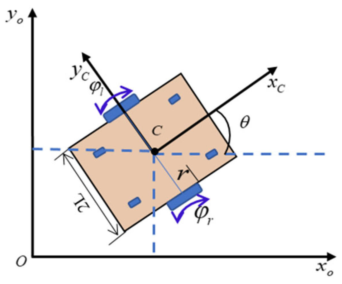
2.1. The Kinematics of the Non-Holonomic Wheeled Mobile Robot (WMR)

Consider an autonomous robot as depicted in Figure 1:

Where: A is the midpoint of two active wheels, C is the coordinates of the center of gravity of the robot, a is the distance between the coordinates of the center of gravity to the wheel axle, $r$ is the radius of the active wheel, 2L is the distance between the two wheels, and m is the mass of the robot.

The robot’s position is determined by a vector $\xi ={\left[x,y,\theta \right]}^T$ ($x,y$ is the C-coordinate).

Consider a robot model with horizontal sliding motion with a speed of $\dot{\eta }$:

$$-\dot{x}\sin (\theta )+\dot{\mathrm{y}}\mathrm{c}\mathrm{o}\mathrm{s}(\theta )=\dot{\eta }$$

(1)

Pure rotational constraints: The active wheels always maintain a contact point. These active wheels cannot slide vertically and can slide horizontally, so we have:

$$\dot{x}\cos (\theta )+\dot{\mathrm{y}}\mathrm{s}\mathrm{i}\mathrm{n}(\theta )+L\dot{\theta }-r{\dot{\phi }}_r=0$$

(2)

$$\dot{x}\cos (\theta )+\dot{\mathrm{y}}\mathrm{s}\mathrm{i}\mathrm{n}(\theta )-L\dot{\theta }-r{\dot{\phi }}_l=0$$

(3)

when $\vartheta =\dot{x}\cos (\theta )+\dot{\mathrm{y}}\mathrm{s}\mathrm{i}\mathrm{n}(\theta )+\dot{\eta }\mathrm{va}\omega =\dot{\theta }$, we have:

$$\begin{array}{l}\vartheta +L\omega -\dot{\eta }=r{\dot{\phi }}_r\\ \vartheta -L\omega -\dot{\eta }=r{\dot{\phi }}_l\end{array}$$

(4)

From (1)–(3), we have the kinematics described in vector form:

$$A(q)\dot{q}=0$$

(5)

Represented by six general coordinates as follows:

$$q={\left[\begin{array}{cc}{\xi }^T& {\phi }^T\end{array}\right]}^T={\left[\begin{array}{cccccc}x& y& \theta & \eta & {\phi }_r& {\phi }_l\end{array}\right]}^T$$

(6)

From (6), (7), and (9), the constraint equation in matrix form is as follows:

$$A(q)\dot{q}=\left[\begin{array}{cccccc}\cos (\theta )& \sin (\theta )& -L& 0& -r& 0\\ \cos (\theta )& \sin (\theta )& L& 0& 0& -r\\ -\sin (\theta )& \cos (\theta )& 0& -1& 0& 0\end{array}\right]{\left[\begin{array}{cccccc}\dot{x}& \dot{y}& \dot{\theta }& \dot{\eta }& {\dot{\phi }}_r& {\dot{\phi }}_l\end{array}\right]}^T$$

(7)

We have $\dot{q}$ of the robot in the original coordinate system determined by the rotation around the Z-axis at an angle $\mathsf{\theta }$, so we have an equation describing the robot’s kinematics:

$$\dot{q}=\left[\begin{array}{ccc}\cos (\theta )& 0& -\sin (\theta )\\ \sin (\theta )& 0& \cos (\theta )\\ 0& 1& 0\end{array}\right]\left[\begin{array}{c}\vartheta \\ \omega \\ \dot{\eta }\end{array}\right]=\left[\begin{array}{c}\dot{x}\\ \dot{y}\\ \dot{\theta }\end{array}\right]=H(q)\vartheta (t)$$

(8)

2.2. Dynamics of Non-Holonomic Wheeled Mobile Robots (WMR)

Dynamics for mobile robots are determined according to the Lagrange method as follows:

$$\frac{d}{dt}\left(\frac{\partial T}{\partial \dot{q}}\right)-\frac{\partial T}{\partial q}=F-A^T(q)\lambda$$

(9)

where $T$ is the Lagrange function: $T=T_c+T_{\omega r}+T_{\omega l}$

The kinetic energy of the mobile robot body:

$$T_c=\frac{1}{2}{m}_c({\dot{x}}^2+{\dot{y}}^2)+\frac{1}{2}{I}_c{\dot{\theta }}^2$$

(10)

The kinetic energy of the left and right wheels, taking into account the sideways sliding motion are:

$$T_{\omega r}=\frac{1}{2}{m}_{\omega }(v_{\omega r}^2+{\dot{\eta }}^2)+\frac{1}{2}{I}_m{\dot{\theta }}^2+\frac{1}{2}{I}_{\omega }{\dot{\phi }}_r^2$$

(11)

$$T_{\omega l}=\frac{1}{2}{m}_{\omega }(v_{\omega l}^2+{\dot{\eta }}^2)+\frac{1}{2}{I}_m{\dot{\theta }}^2+\frac{1}{2}{I}_{\omega }{\dot{\phi }}_l^2$$

(12)

From Equations (12)–(19), we have the kinetic energy total:

$$T=\frac{1}{2}{m}_t\left({\dot{x}}^2+{\dot{y}}^2\right)+\frac{1}{2}{m}_{\omega }\left({\dot{\phi }}_r^2+{\dot{\phi }}_l^2\right)+m_{\omega }{\dot{\eta }}^2+\frac{1}{2}I{\dot{\theta }}^2+\frac{1}{2}{I}_{\omega }\left({\dot{\phi }}_r^2+{\dot{\phi }}_l^2\right)$$

(13)

where $m_t=m_c+2m_{\omega };I=I_c+2I_m$ and $\dot{\theta }=\omega$.

Using Equation (19) with the Lagrange method to the equation of motion of mobile robots:

$$\{\begin{array}{c}{m}_t\ddot{x}=F_1-C_1\\ m_t\ddot{y}=F_2-C_2\\ \begin{array}{l}I\ddot{\theta }=F_3-C_3\\ 2m_{\omega }\ddot{\eta }=F_4-C_4\end{array}\\ (m_{\omega }{r}^2+I_{\omega }){\ddot{\phi }}_r={\tau }_r-C_5\\ (m_{\omega }{r}^2+I_{\omega }){\ddot{\phi }}_l={\tau }_l-C_6\end{array}$$

(14)

Identify constraints in the kinematic model:

$$-A^T(q)\lambda ={\left[\begin{array}{cccccc}{C}_1& C_2& C_3& C_4& C_5& C_6\end{array}\right]}^T$$

(15)

From Equations (13)–(15), determine the dynamic equation of a non-holonomic mobile robot that can be described as:

$$M(q)\ddot{q}+C(q,\dot{q})\dot{q}+G(q,\dot{q})sng(\dot{q})+{\tau }_d=-A^T(q)\lambda +B(q)\tau$$

(16)

where $M(q)$ is a positive definite inertial matrix, $C(q,\dot{q})$ is the Centripetal and Coriolis matrix, $G(q,\dot{q})sng(\dot{q})$ is the friction matrix, ${\tau }_d$ is the unknown noise component of the system, $B(q)$ is the input matrix, $\lambda$ is the Lagrange multiplier, $\tau$ is the motion control torque for mobile robots, $A(q)$ is the binding matrix, and $\dot{q}$ and $\ddot{q}$ represent the generalized velocity and acceleration vectors, respectively, with:

$$\begin{gathered} M(q)=\left[\begin{array}{cccccc}{m}_t& 0& 0& 0& 0& 0\\ 0& m_t& 0& 0& 0& 0\\ 0& 0& I& 0& 0& 0\\ 0& 0& 0& 2m_{\omega }& 0& 0\\ 0& 0& 0& 0& (m_{\omega }{r}^2+I_{\omega })& 0\\ 0& 0& 0& 0& 0& (m_{\omega }{r}^2+I_{\omega })\end{array}\right], \\ C(q,\dot{q})=\left[\begin{array}{cccccc}0& 0& 0& 0& 0& 0\\ 0& 0& 0& 0& 0& 0\\ 0& 0& 0& 0& 0& 0\\ 0& 0& 0& 0& 0& 0\\ 0& 0& 0& 0& 0& 0\\ 0& 0& 0& 0& 0& 0\end{array}\right], \end{gathered}$$

$$B(q)=\left[\begin{array}{cc}0& 0\\ 0& 0\\ 0& 0\\ 0& 0\\ 1& 0\\ 0& 1\end{array}\right],A{(q)}^T\lambda =\left[\begin{array}{ccc}\cos (\theta )& \cos (\theta )& -\sin (\theta )\\ \sin (\theta )& \sin (\theta )& \cos (\theta )\\ -L& L& a\\ 0& 0& 1\\ -r& 0& 0\\ 0& -r& 0\end{array}\right]\left[\begin{array}{c}{\lambda }_1\\ {\lambda }_2\\ {\lambda }_3\end{array}\right], \tau =\left[\begin{array}{c}{\tau }_r\\ {\tau }_l\end{array}\right]$$

$$G(q,\dot{q})sng(\dot{q})={\left[\begin{array}{cccccc}{F}_1& F_2& F_3& F_4& 0& 0\end{array}\right]}^T$$

where $m_t$ is the mass of the robot, $I$ is the inertia according to the center of gravity C of the robot, $F_1,F_2,F_3,F_4$ are the friction force in the direction of translational motion, rotational direction, and horizontal sliding friction, respectively, and ${\tau }_l$ and ${\tau }_l$ are the left wheel torque and right wheel torque, respectively.

From Equations (11) and (12), we can prove that the transformation matrix $H(q)$ is the empty space of the constraint matrix $A(q)$ so we will have:

$$H(q)A{(q)}^T=0$$

(17)

We differentiate Equation (12), so we have:

$$\ddot{q}=\dot{H}(q)\upsilon (t)+H(q)\dot{\upsilon }(t)$$

(18)

From there, we have the system’s dynamic equation as follows:

$$\overline{M}(q){\dot{x}}_2+\overline{C}(q,\dot{q})x_2+\overline{G}(q,\dot{q})\mathrm{sgn}(\upsilon )+{\overline{\tau }}_d=\overline{B}(q)\tau$$

(19)

where $\overline{M}(q)=H(q)M(q)H(q)$ $\overline{C}(q,\dot{q})=H(q)\left[M(q)\dot{H}(q)+C(q,\dot{q})H(q)\right]$,$\overline{B}(q)=H(q)B(q)$$\overline{G}(q,\dot{q})\mathrm{sgn}(\upsilon )=H(q)G(q,\dot{q})sng(\upsilon )$, and ${\overline{\tau }}_d=H(q){\tau }_d$.

Comment: From Equation (23), we see that the dynamic model of the WMR has more variables to control than the number of control variables. Uncertainty and noise components in the system include:

-

Vehicle mass and moment of inertia are uncertain, so the inertia matrix is considered uncertain.

-

When the vehicle moves on different floors, especially slippery and wet floors, it is easy for the wheel to slip, affecting the road trajectory, or when the vehicle moves at a fast speed into curves, it can easily cause wheel slippage. The friction between the wheel and the floor will change, causing interference that greatly affects the position and direction of the vehicle.

-

In addition, there still exists noise due to model errors and measurement noise. These are also issues considered when designing the control for WMRs. In this study, we use the kinematic and dynamic model of a mobile robot when there is a side slip as the control object so that this WMR follows a given trajectory and can compensate for the side slip using DSC, AFDSC, and AFNNDSC.

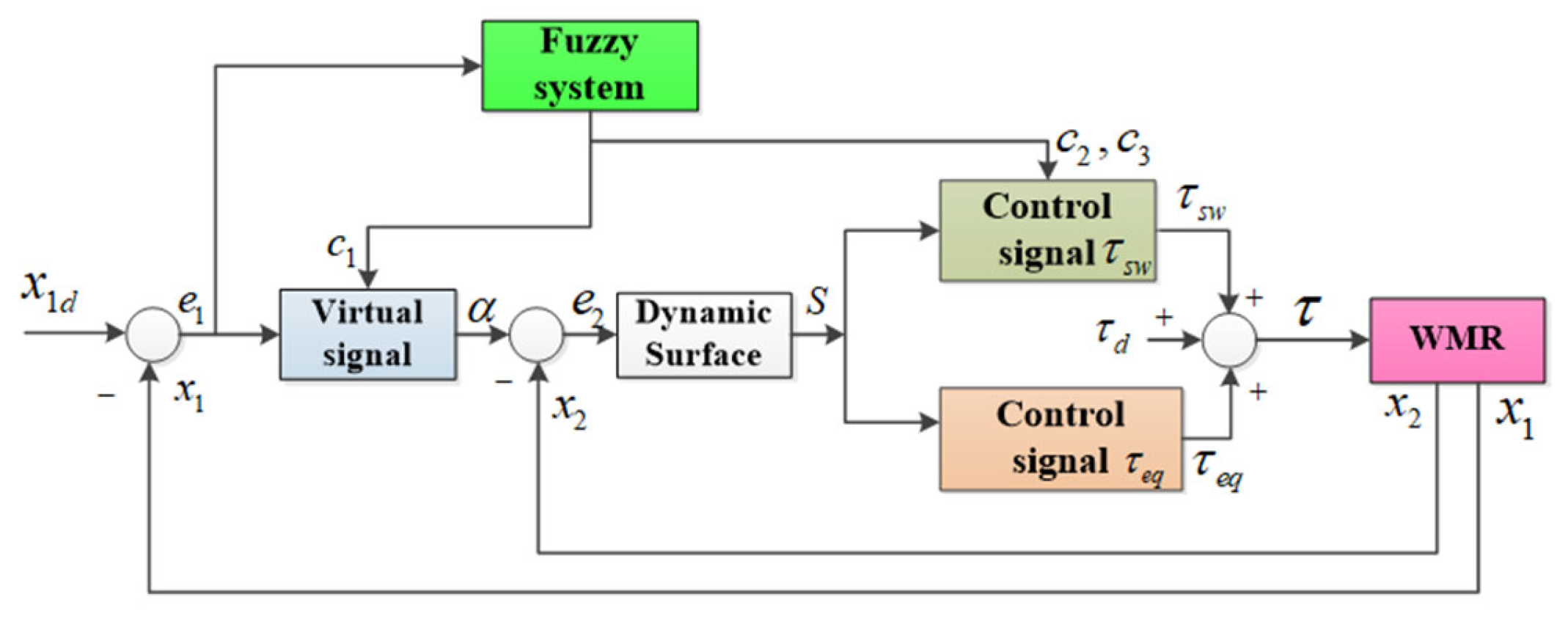
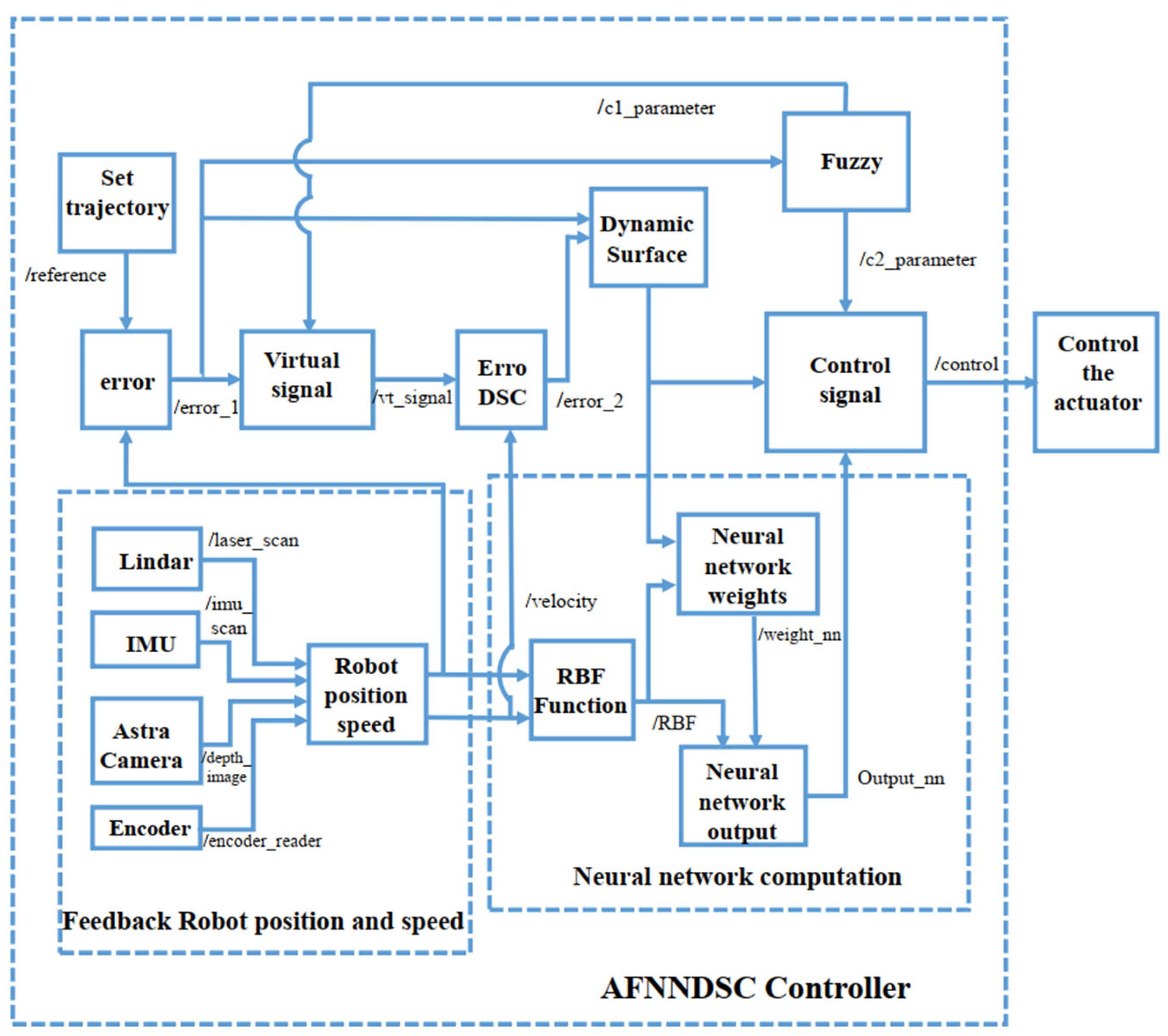
3. Design the Adaptive Fuzzy Neural Network Dynamic Surface Controller (AFNNDSC)

3.1. Dynamic Sliding Control Algorithm

3.1.1. Building a Dynamic Sliding Surface Trajectory Control Algorithm for WMRs

The DSC technique is developed based on a multistage sliding controller and backstepping techniques [14,15,19]. Not only does it retain the advantages of dealing with uncertain components in the system model, but DSC also overcomes the disadvantages of these two methods by integrating a low-pass filter into the controller [41].

First of all, the goal of designing the controller is that the robot can follow the trajectory quickly and accurately while ensuring the stability of the system. A DSC controller for WMRs is focused on design research. To simplify calculations and prove the stability of the control system, the system’s state variables are set as follows:

According to document [14], the proposed state variables are as follows:

$$\{\begin{array}{l}{x}_1=q={\left[\begin{array}{lll}x\hfill & y\hfill & \theta \hfill \end{array}\right]}^T\hfill \\ x_2=\vartheta (t)=\left[\begin{array}{ccc}\upsilon & \omega & \dot{\eta }\end{array}\right]\hfill \end{array}$$

(20)

Combining kinematic Equations (12) and (24), we will have:

$${\dot{x}}_1=H(q)x_2$$

(21)

From Equations (23) to (25), we get the state model:

$$\{\begin{array}{l}{\dot{x}}_1=H(q)x_2\hfill \\ \overline{M}(q){\dot{x}}_2+\overline{C}(q,\dot{q})x_2+\overline{G}(q,\dot{q})\mathrm{sgn}(x_2)+{\overline{\tau }}_d=\overline{B}(q)\tau \hfill \end{array}$$

(22)

The first, set $e_1=x_1-x_{1d}$, is the trajectory error vector. There, the

$$x_{1d}=q_d={\left(\begin{array}{lll}{x}_d\hfill & y_d\hfill & {\theta }_d\hfill \end{array}\right)}^T \mathrm{is\; the\; set\; trajectory.}$$

(23)

The control goal is to ensure that $x_1$ reaches a farvalue $x_{1d}$ meaning that $e_1$ approaches zero.

$$\mathrm{Derivative} {\mathrm{e}}_1: {\dot{e}}_1={\dot{x}}_1-{\dot{x}}_{1d}=H(q)x_2-{\dot{x}}_{1d}$$

(24)

Assume that the control signal is virtual in the design of the DSC controller. It is the input to the first-order low-pass filter with the expression.

$$\alpha =-H{(q)}^{-1}\left(c_1{e}_1-{\dot{x}}_{1d}\right)$$

(25)

where $c_1=\left(\begin{array}{ccc}{c}_{1x}& 0& 0\\ 0& c_{1y}& 0\\ 0& 0& c_{1\theta }\end{array}\right)$ is the appropriate diagonal constant matrix value whose elements are positive values.

After calculating the virtual control law, $\alpha$ is passed through a first-order low-pass filter to calculate the derivative value for the virtual control signal.

$$T{\dot{\alpha }}_r+{\alpha }_r=\alpha$$

(26)

where $T$ is chosen small enough not to increase the calculation time of DSC.

$${\alpha }_f(s)=\frac{\alpha (s)}{Ts+1},{\dot{\alpha }}_f=\frac{\alpha -{\alpha }_f}{T}$$

(27)

To demonstrate the availability of virtual control signals, choose the first Lyapunov function:

$$V_1=\frac{1}{2}{e}_1^T{e}_1$$

(28)

Consider the derivative of $V_1$.

$${\dot{V}}_1=e_1{}^T{\dot{e}}_1=e_1{}^T\left(H(q)x_2-{\dot{x}}_{1d}\right)=-e_1{}^T{c}_1{e}_1+e_1{}^T\left(c_1{e}_1+H(q)x_2-{\dot{x}}_{1d}\right)$$

(29)

If you watch $x_2=\alpha$, then ${\dot{V}}_1=-e_1{}^T{c}_1{e}_1+e_1{\dot{c}}_1\left(e_1-e_1\right)$.

It can be seen from Equation (29) with a virtual control value from Equation (25), ${\dot{V}}_1=-e_1^T{c}_1{e}_1\le 0$ and condition ${\dot{V}}_1=-e_1^T{c}_1{e}_1\le 0$ is satisfied.

Next, the sliding control technique is designed to obtain the control signal of the system. This control signal must also ensure that the virtual control signal achieves the ideal value. The definition of system virtual control signal bias:

$$e_2=x_2-{\alpha }_f$$

(30)

$$\mathrm{Choose\; slide:} S=\lambda e_1+H(q)e_2$$

(31)

where $\lambda$ is the coefficient of the sliding surface.

The derivative of S is calculated (36)

$$\dot{S}=\lambda {\dot{e}}_1+H(q){\dot{e}}_2+\dot{H}{e}_2=\lambda {\dot{e}}_1+\dot{H}(q)(q)e_1+H(q)\left(\overline{M}{(q)}^{-1}\left(-\overline{C}(q,\dot{q})x_2-\overline{G}(q,\dot{q})\mathrm{sgn}(x_2)+\overline{B}(q)\tau \right)-{\dot{\alpha }}_f\right)$$

(32)

As mentioned above, one of the advantages of a DSC controller is its ability to avoid the “term explosion” phenomenon that occurs when the calculation of the derivative of a virtual control signal is repeated at every cycle. Therefore, the value of alpha is obtained from the first-order filter (31). To ensure the stability of the system and calculate the control signal, the second Lyapunov function is chosen.

$$V_2=\frac{1}{2}{S}^{T}S$$

(33)

The system’s control signal will be calculated in the form of a sliding controller to increase the system’s robustness against noise. Therefore, the control signal will include two components TT which is the control signal to keep the system state on the sliding surface TR obtained from the condition $\dot{S}=0$.

$${\tau }_{eq}=-\overline{B}{(q)}^T{\left(\overline{B}(q)\overline{B}{(q)}^T\right)}^{-1}\left(\overline{M}(q)\left(H{(q)}^{-1}\left(\lambda {\dot{e}}_1+\dot{H}(q)e_2\right)-{\dot{x}}_{2d}\right)-\overline{C}(q,\dot{q})x_2-\overline{G}(q,\dot{q})\mathrm{sgn}(x_2)\right)$$

(34)

However, ${\tau }_{eq}$ is only effective when the system is on the sliding surface. Therefore, the control signal ${\tau }_{sw}$ is used, as it is capable of driving the state of the system towards the sliding surface. The expression of ${\tau }_{\tau w}$ is selected as follows:

$${\tau }_{sw}=-\overline{B}{(q)}^T{\left(\overline{B}(q)\overline{B}{(q)}^T\right)}^{-1}\overline{M}(q)H(q)H{(q)}^{-1}\left(c_2\mathrm{sgn}(S)+c_{2}S\right)$$

(35)

where $c_2=\left(\begin{array}{ccc}{c}_{2x}& 0& 0\\ 0& c_{2y}& 0\\ 0& 0& c_{2\theta }\end{array}\right) \mathrm{and} c_3=\left(\begin{array}{ccc}{c}_{3x}& 0& 0\\ 0& c_{3y}& 0\\ 0& 0& c_{3\theta }\end{array}\right)$ are positive definite coefficient matrices. Finally, the control signal of the system is the sum of ${\tau }_{eq},{\tau }_{sw}$:

$$\tau ={\tau }_{eq}+{\tau }_{sw}$$

(36)

Theorem 1.

The WMR described using the model (23) is controlled by (36) with ${\tau }_{eq}$ determined by (30) and ${\tau }_{sw}$ (35) ensuring the closed system is stable and the tracking error approaches 0.

Proof.

Derivative $V_2$:

$${\dot{V}}_2=S^T\dot{S}$$

(37)

Using (36), ${\dot{V}}_2$ becomes

$${\dot{V}}_2=S^T\left(\lambda {\dot{e}}_1+\dot{H}(q)e_2+H(q)\left(\overline{M}{(q)}^{-1}\left(-\overline{C}(q)x_2-\overline{G}(q,\dot{q})\mathrm{sgn}(x_2)+\overline{B}(q)\tau \right)-{\dot{\alpha }}_f\right)\right)$$

(38)

with control signal (34)–(38) then $x_{2d}={\dot{\alpha }}_f,$ the derivative of $V_2$ can be rewritten.

$${\dot{V}}_2=-S^T{c}_2\mathrm{sgn}(S)-S^T{c}_{3}S$$

(39)

Noise value ${\overline{\tau }}_d$ is blocked $\left|{\overline{\tau }}_d\right|\le \lambda$ is an uncertain noise value so it does not appear in the controller expression. Choosing $c_1,c_3$ appropriately, we have

$$\dot{V}=-S^T{c}_2\mathrm{sgn}(S)-S^T{c}_{3}S\le 0$$

(40)

□

The advantage of the DSC method is to increase the adaptability of the system and reduce the amount of controller computation. The control signal used contains a sliding component, hence the robust stability of the SMC. The low-pass filter used not only filters out endogenous high-frequency noise but also provides information about the derivative of the virtual control signal. Therefore, calculating the derivative of the virtual control signal becomes unnecessary. The control signal used contains a slip component, hence the robust stability of the SMC. The low-pass filter used not only fil-ters out endogenous high-frequency noise but also provides information about the de-rivative of the virtual control signal. Therefore, calculating the derivative of the virtu-al control signal becomes unnecessary, which eliminates the disadvantages of MSSC and backstepping techniques. However, this method is only applicable when model errors and disturbances are small; on the other hand, the chattering phenomenon caused by the sliding controller structure is unavoidable. Furthermore, the control quality of the system depends a lot on the choice of controller parameters, especially the parameters that directly affect the system’s traction on the sliding surface.

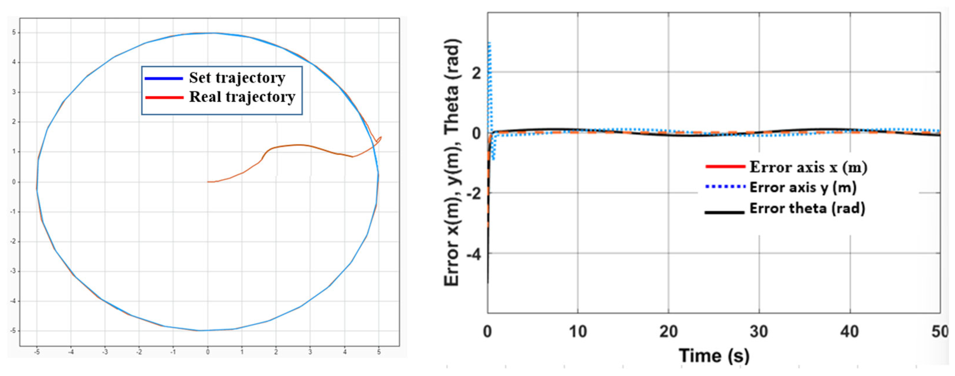
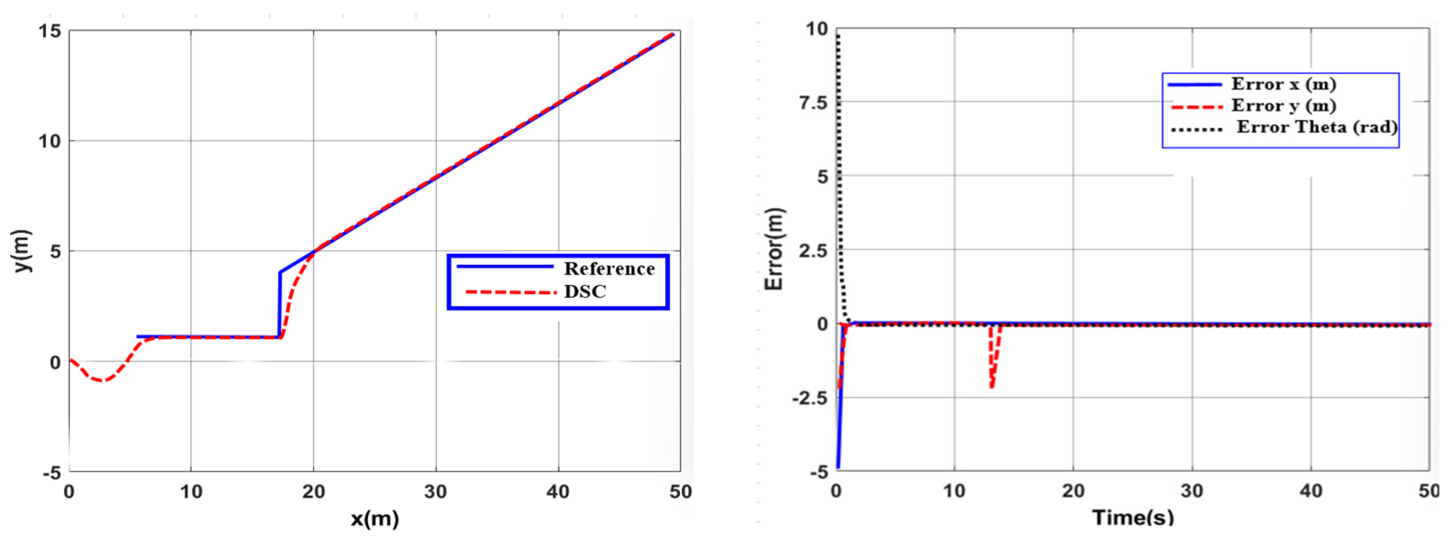
3.1.2. Simulation to Verify the Algorithm

Block diagram simulating system structure and DSC controller is shown Figure 2 and Figure 3:

a. 

In case there is no interference

Choose a circular orbit with the following equation of motion: $x=5\cos (\frac{\pi }{15}t);$ $y=5\sin (\frac{\pi }{15}t); \theta =\frac{\pi }{15}t+\frac{\pi }{2}$. DSC control parameter set: $C_1=diag(11,11,11)$; $C_2=C_3=diag(15,15,15)$, $\lambda =diag(10,10,10)$. Tracking trajectory and tracking error when using DSC with circular orbit is shown Figure 4 and Figure 5.

Choose a trajectory that is a curved line: $x_1=5*3t,y_1=1,{\theta }_1=a\tan (5/3);$ $x_2=5*3t,y_2=t,{\theta }_2=a\tan (5/3)$. DSC control parameter set: $\lambda =diag(10,10,10)$; $C_1=diag(11,11,11)$; $C_2=C_3=diag(15,15,15)$.

Comment: In the initial stage, when the robot’s position is not yet on the trajectory, the DSC controller acts to bring the robot to orbit at a fast speed and the transient component is insignificant. The trajectory tracking quality is good with the error kept at a very small value, approximately $x_e=0.035(m);y_e=0.052(m);{\theta }_e=0.026(rad)$.

b. 

In case of interference

As described in the control algorithm design section, the ${\overline{\tau }}_d$ component does not appear in the controller expression when designing with the mathematical model (23). However, in reality, this noise component still affects the system and there is no method to accurately measure this value. To verify the effectiveness, in the simulation of the control algorithm, this ${\overline{\tau }}_d$ component will appear in the system to evaluate the noise resistance of the controllers. In this section, it is assumed that the impact noise is random numbers that impact the system and satisfy the condition that the noise is blocked $\Vert {\overline{\tau }}_d\Vert <\lambda$.

Comment on the results Figure 6: The DSC controller not only greatly reduces the “chattering” phenomenon but also reduces the influence of noise as well as faster response time by using input low-pass filters, capturing errors, suppression, and minimum transient time. Therefore, DSC is chosen as the foundation to build adaptive controllers. To reduce chattering due to noise, the effect of the sign() function when the system contains uncertain components will be approximated by an online artificial neural network and compensated in the control law. A new adaptive DSC for WMRs based on a fuzzy logic system and artificial neural network overcomes the disadvantages of DSC.

3.2. Adaptive Fuzzy Logic Dynamic Surface Controller for (AFDSC)

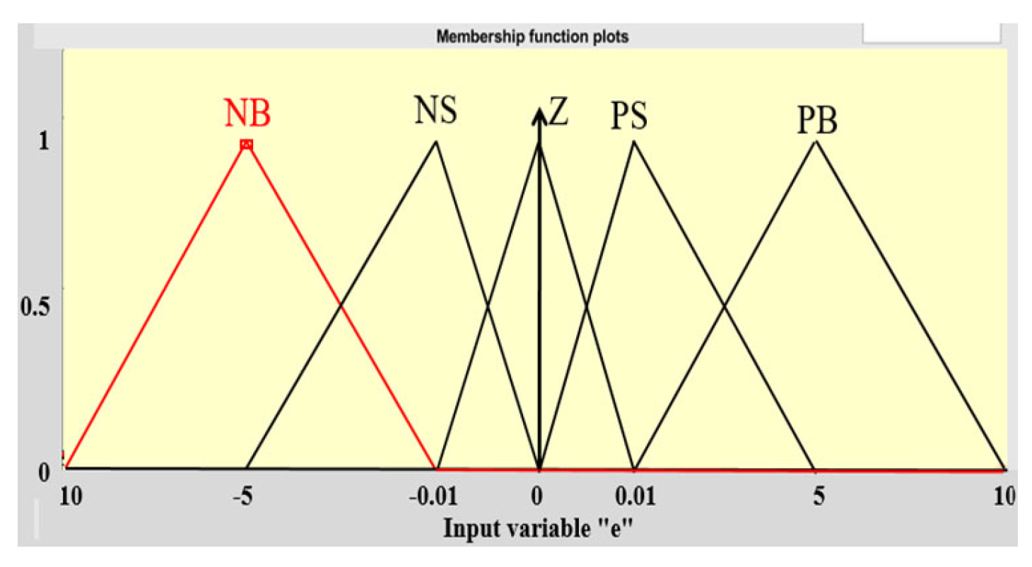
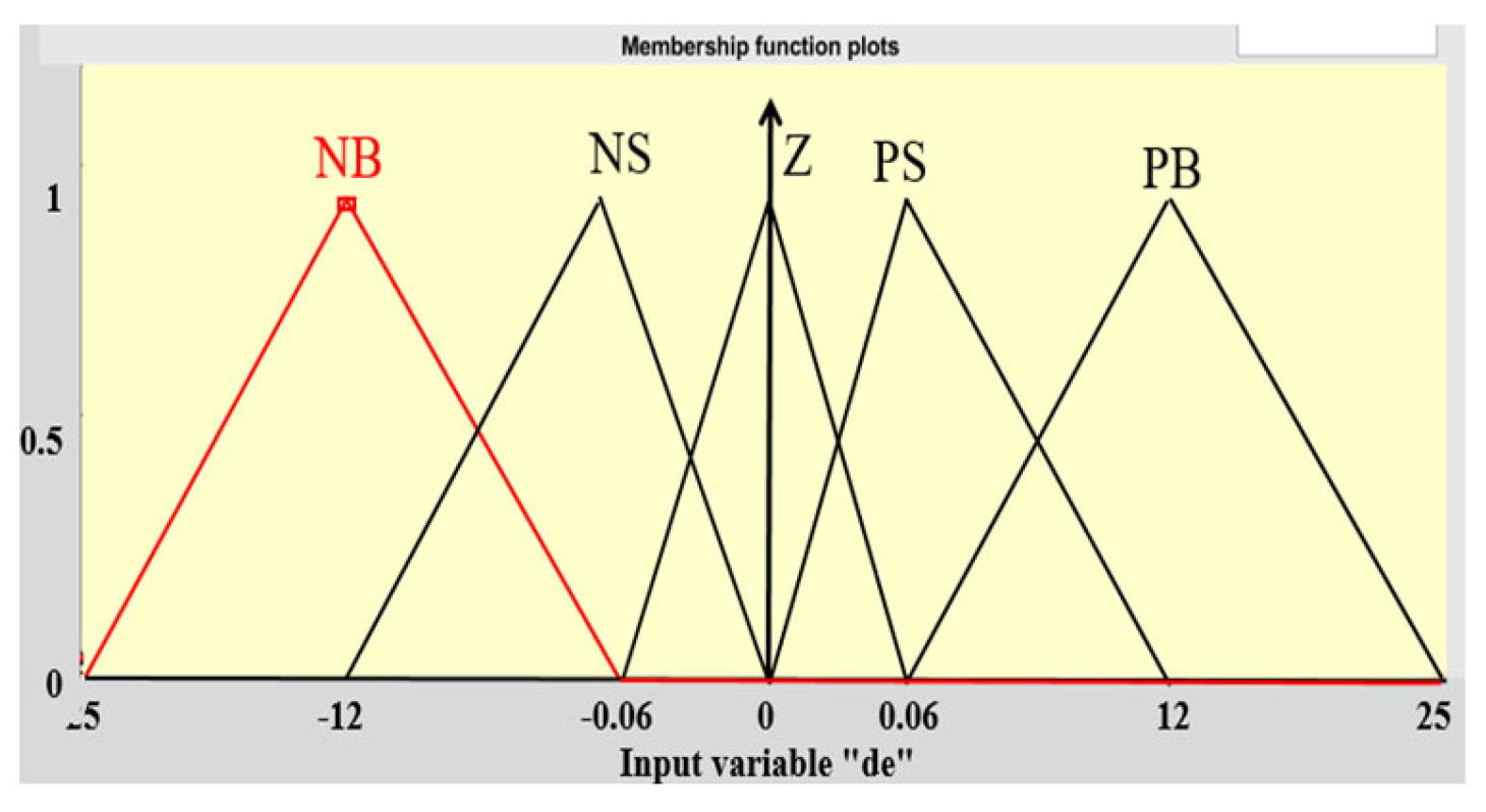
3.2.1. The Adaptive Fuzzy Logic Dynamic Surface Controller

The strength of the DSC controller is its stability with non-stationary system parameters (uncertain parameters change within limits), but this strength is only promoted when the system state is on the sliding surface or the vicinity of the sliding surface. The structure diagram of the fuzzy DSC system is shown in Figure 7 below:

Input of fuzzy correction and derivative. The input fuzzy sets and output constants are selected through the experiment. The fuzzy set for the input linguistic variables is shown in Figure 7. The input linguistic variables are shown in

Table 1. Fuzzy sets of input linguistic variables.

Language Variation e	Language Variation $\dot{\mathit{e}}$	Meaning
NB	NB	Negative big
NS	NS	Negative small
Z	Z	Zezo
PS	PS	Positive small
PB	PB	Positive big

.

Variable language of $e$: NB, NS, Z, PS, PB

Variable language of $\dot{e}$: NB, NS, Z, PS, PB

The first output of the fuzzy set is the parameter $c_{1i}(i=x,y,\theta )$ and it is also a parameter of the sliding surface. The remaining output is the parameter $c_{2i}(i=x,y,\theta )$ and $c_{3i}(i=x,y,\theta )$. To reduce the complexity of AFDSC, these remaining parameters are chosen to be equal. The basic inference rule system is shown in

Table 2. Base inference rule system for $c_1(c_2,c_3)$.

${\dot{e}}_1$	$e_1$
	NB	NS	Z	PS	PB
NB	M(M)	S(B)	VS(VB)	S(B)	M(M)
NS	B(S)	M(M)	S(B)	M(M)	B(S)
Z	VS(VB)	B(S)	M(M)	B(S)	VS(VB)
PS	B(S)	M(M)	S(B)	M(M)	B(S)
PB	M(M)	S(B)	VS(VB)	S(B)	M(M)

Fuzzy sets for input are shown in Figure 8 and Fuzzy sets for input are shown in Figure 9.

From Formula (49), we see that the $(c_2,c_3)$ component is a parameter that affects the speed of approaching the sliding surface and controls the state of the system located on the sliding surface, to simplify the selection of values for fuzzy sets and block reduction. The amount of calculation is not necessary, so the $(c_2,c_3)$ outputs are chosen to be equal and the basic inference rule system of the fuzzy regulator for these two outputs is shown in

Table 3. Output values $c_1,c_2,c_3$.

Variable Output Language	Meaning	$\mathbf{Output} \mathbf{Value} \mathbf{for} {\mathit{c}}_1$	$\mathbf{Output} \mathbf{Value} \mathbf{for} {\mathit{c}}_2$$\mathbf{and} {\mathit{c}}_3$
VS	Verry small	1.5	20
S	Small	4.25	25
M	medium	6.5	30
B	Big	8	35
VB	Verry big	10	40

Membership function form: trimf with parameters. Fuzzy controller using composition rule SumPROD.

.

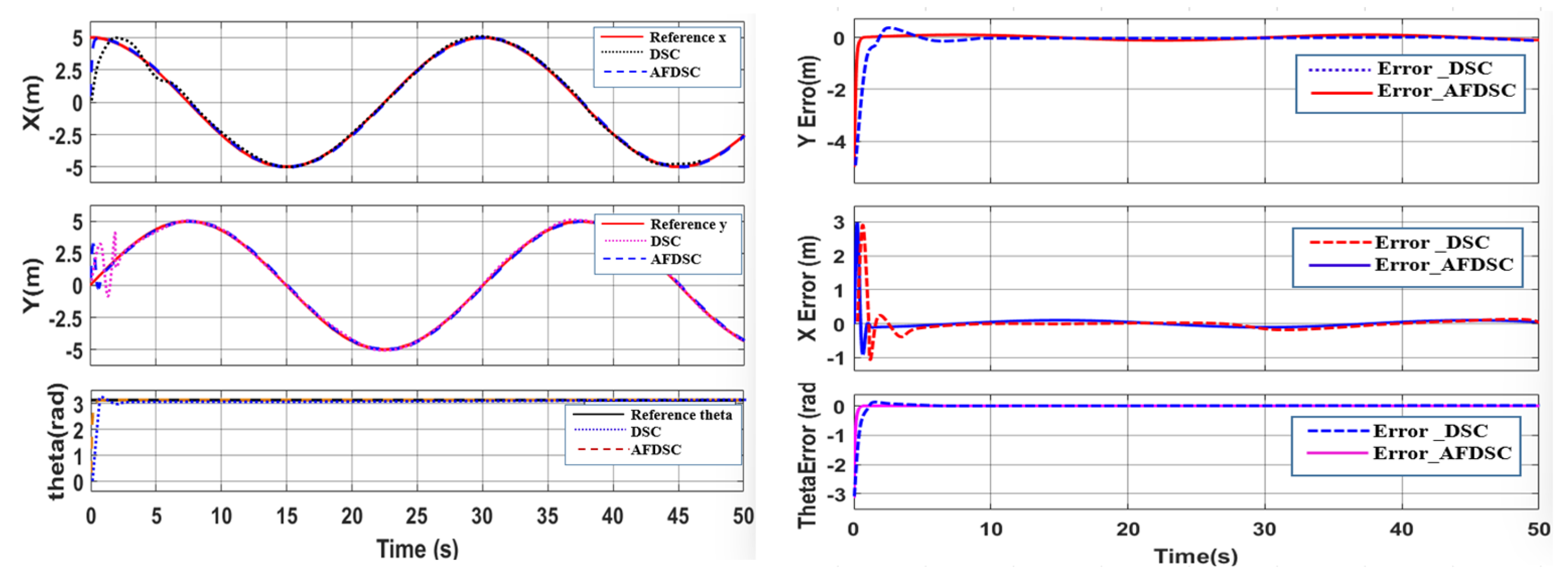
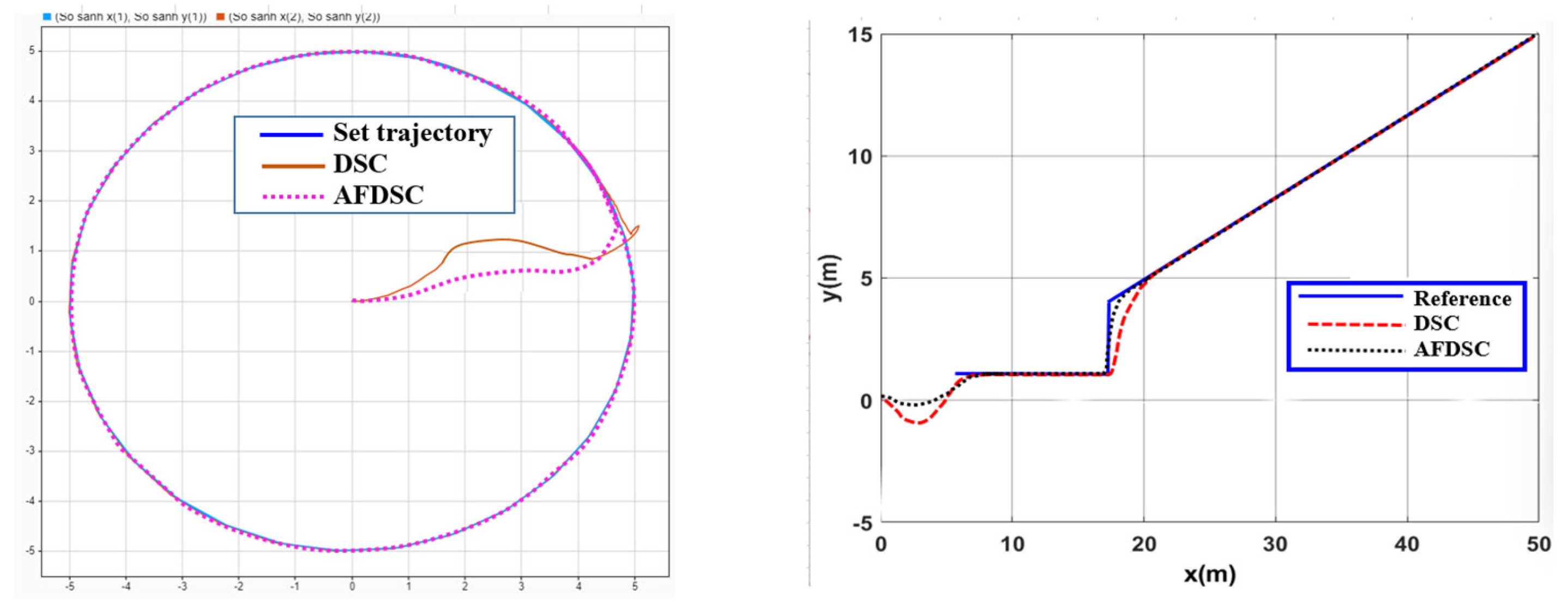
3.2.2. Simulation to Verify the Controller AFDSC

The simulation used a self-propelled robot model using the Matlab/Simulink tool. To demonstrate the effectiveness of the proposed AFDSC algorithm, external random noise was added to the model as follows Figure 10:

Conducting simulations and evaluating the proposed new algorithm with a circular trajectory, the WMR will move from an initial point (0,0) inside the circle in the original coordinate system. The trajectory for the robot to follow according to the origin coordinate system is given by: $x=5\cos (\frac{\pi }{15}t);y=5\sin (\frac{\pi }{15}t); \theta =\frac{\pi }{15}t+\frac{\pi }{2}$ Kinetic model parameters: $\mathrm{m}=13 \mathrm{kg}; \mathrm{J}=0{.56 \mathrm{kgm}}^2, r=0.08 \mathrm{m}, 2\mathrm{L}=0.6 \mathrm{m},$ $\lambda =diag(10,10,10)$.

Comment: Figure 11 above describes the trajectory motion of the WMR with DSC and AFDSC controllers. It can be seen that both controllers ensure the WMR follows the set orbit but AFDSC gives better tracking quality. Specifically, with the same initialization conditions, FWOMR with AFDSC reaches the reference orbit after about 0.2 s, while with DSC it takes nearly 0.5 s. The fuzzy rules are designed to update the parameters of DSC online whenever there is a change in the two inputs of the fuzzy regulator, the bias and the bias derivative. The new proposed AFDSC set ensures the quality of tracking the system’s preset orbit better than the DSC set: the time to reach the set trajectory is faster and the tracking error is also smaller.

The parameters ($c_1,c_2,c_3$) of the online tuning AFDSC controller are shown in Figure 12, Figure 13 and Figure 14.

Figure 15 depicts the movement of the WMR with two different trajectories (curved trajectory and circular trajectory). The effectiveness of the algorithm can be clearly seen when the robot’s orbit follows the trajectory set very closely in both cases.

3.3. Adaptive Fuzzy Neural Network Dynamic Surface Controller for (AFNNDSC)

An AFNNDSC improves the chattering phenomenon caused by the effects of nonlinear uncertainties and noise when the system contains many nonlinear uncertainties, wheel slippage, and noise with variable magnitude. The proposed solution is that estimating the model error and compensating in the controller component will ensure improvement in the quality of this controller. Thus, controller parameter adjustment combined with online uncertainty compensation will certainly significantly improve the quality of the WMR control system. Figure 16 is the structure diagram of the AFNNDSC tracking control system.

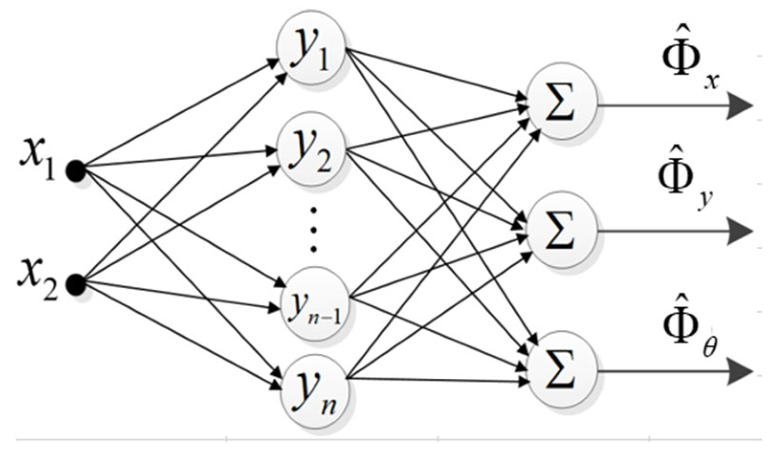
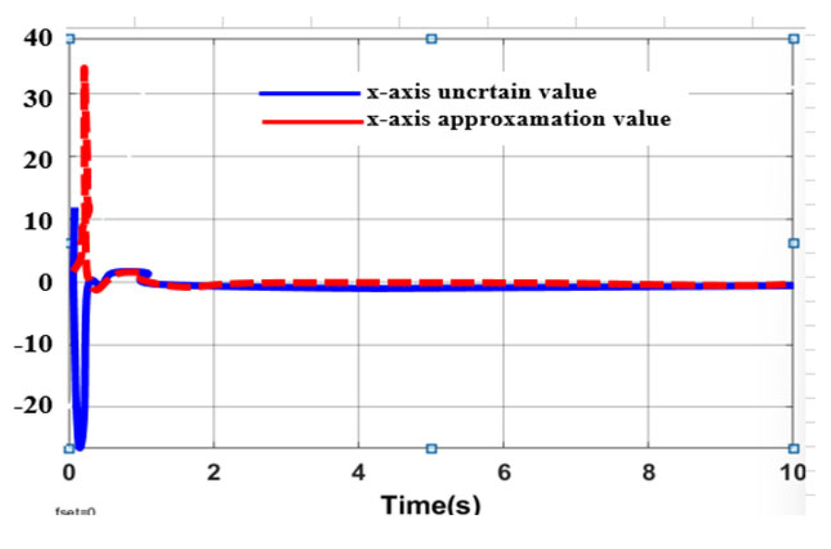
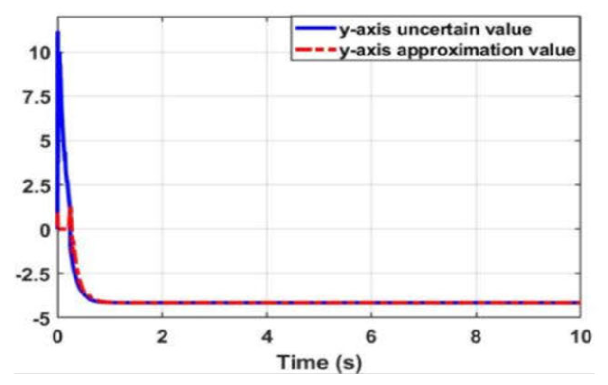
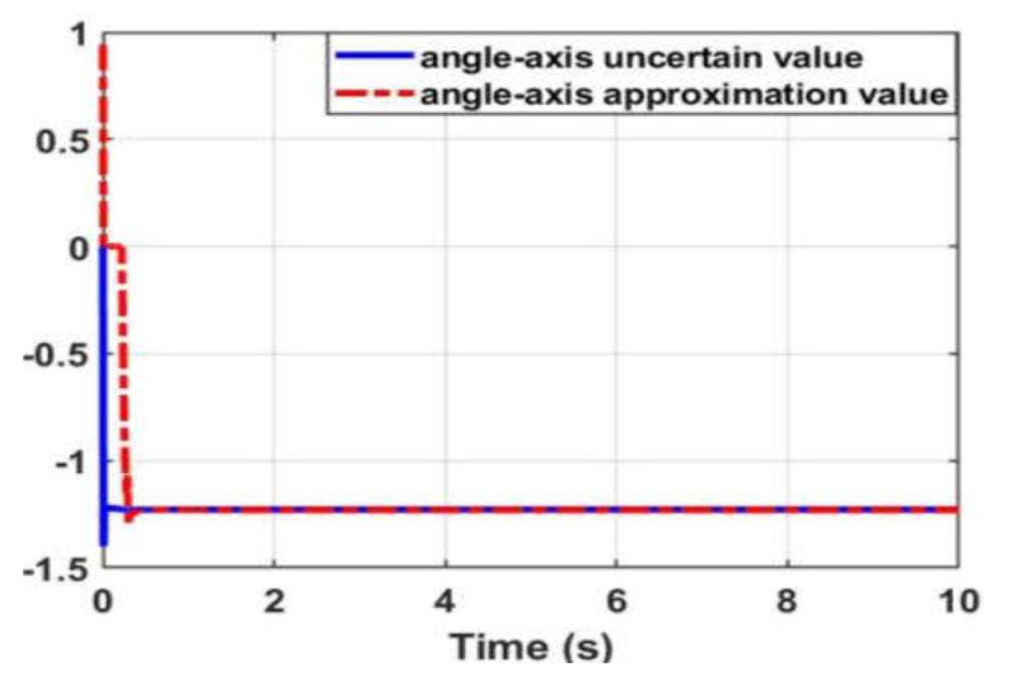
3.3.1. Approximation of WMR Model Uncertainty Component Using Radial Neural Network

Neural networks combined with control methods are considered an effective solution to solve control problems for objects with uncertain models and affected by disturbances. Neural networks can learn the forward kinematics and inverse kinematics characteristics of complex objects, providing an alternative method for controllers to adapt to environmental changes. The basic advantage of this network is that RBF neurons are smooth, differentiable functions, thus ensuring a fast convergence speed and being able to use different training methods. That is why radial neural networks are applied to further improve control quality.

The uncertainty components will be approximated by a neural network to minimize the impact of this phenomenon as follows:

$$\mathrm{\Phi }=-\overline{M}{(q)}^{-1}\left(\overline{C}(q,\dot{q})x_2-\overline{G}(q,\dot{q})\mathrm{sgn}\left(x_2\right)+{\overline{\tau }}_d\right)$$

(41)

is a vector value of dimension (3 × 1) containing the uncertain components of the WMR.

The system of equations describing the WMR is rewritten as:

$$\{\begin{array}{l}{\dot{x}}_1=H(q)x_2\hfill \\ {\dot{x}}_2=\mathrm{\Phi }+\overline{M}{(q)}^{-1}\overline{B}(q)\tau \hfill \end{array}$$

(42)

Carrying out the same calculation steps as the previous section for the controller design, the derivative of the sliding surface becomes:

$$\dot{S}=\lambda {\dot{e}}_1+H(q){\dot{e}}_2+\dot{H}(q)e_2=\lambda {\dot{e}}_1+H(q)e_2+H(q)\left(\mathrm{\Phi }+\overline{M}{(q)}^{-1}\overline{B}(q)\tau -{\dot{x}}_{2d}\right)$$

(43)

System control signals:

$$\tau ={\tau }_{eq}+{\tau }_{sw}$$

(44)

with:

$${\tau }_{eq}=-\overline{B}{(q)}^T{\left(\overline{B}(q)\overline{B}{(q)}^T\right)}^{-1}\overline{M}(q)\left(H{(q)}^{-1}\left(\lambda {\dot{e}}_1+\dot{H}(q)e_2\right)-{\dot{x}}_{2d}+\widehat{\mathrm{\Phi }}\right)$$

(45)

$${\tau }_{sw}=-\overline{B}{(q)}^T{\left(\overline{B}(q)\overline{B}{(q)}^T\right)}^{-1}\overline{M}(q)H{(q)}^{-1}\left(c_2\mathrm{sgn}(S)+c_{3}S\right)$$

(46)

where $\widehat{\mathrm{\Phi }}={\left[\begin{array}{lll}{\widehat{\mathrm{\Phi }}}_x\hfill & {\widehat{\mathrm{\Phi }}}_y\hfill & {\widehat{\mathrm{\Phi }}}_{\theta }\hfill \end{array}\right]}^T$ is the output vector of a neural network trained online to approximate the uncertain components of the system.

The radial neural network consists of three layers: input layer, hidden layer, and output layer shown in Figure 17. The hidden layer neuron nuclei are calculated using the radial radius function. The hidden layer contains a sequence of called computational units and hidden neural kernels. Each kernel contains a vector which is the center parameter of the neuron kernel and it has the same direction as the input vector value. The input vectors chosen are the robot’s states; in this case, the input vectors are the robot’s position and velocity vectors. $x_1={\left[\begin{array}{lll}x\hfill & y\hfill & \theta \hfill \end{array}\right]}^T$, $x_2={\left[\begin{array}{lll}{v}_x\hfill & v_y\hfill & \begin{array}{cc}\omega & \eta \end{array}\hfill \end{array}\right]}^T$. The radial radius function is used to calculate the output of the hidden layer of a neural network based on its ability to approximate uncertain nonlinear functions.

Each output of the neuron kernel in the hidden layer will have a corresponding weight value.

The weight matrix is defined by the matrix. $\mu =\left[\begin{array}{ccc}{\mu }_{11}& {\mu }_{12}& {\mu }_{13}\\ {\mu }_{21}& {\mu }_{22}& {\mu }_{23}\\ ⋮& ⋮& ⋮\\ {\mu }_{n1}& {\mu }_{n2}& {\mu }_{n3}\end{array}\right]$ has size (n × 3) where n is the number of neuron cores, $\gamma ={\left[\begin{array}{llll}{\gamma }_1\hfill & {\gamma }_2\hfill & \cdots \hfill & {\gamma }_n\hfill \end{array}\right]}^T$ is a vector containing the output values of the neuron nuclei.

Select values to calculate the adaptive law for $\widehat{\mathrm{\Phi }}$

$$\mathrm{\Phi }={\mu }^T\gamma +\epsilon \mathrm{and} \widehat{\mathrm{\Phi }}={\widehat{\mu }}^T\gamma$$

(47)

with $\mathrm{\Phi }$ being the ideal value of the system’s uncertainty component, so the controller can ensure control quality as in the case of a deterministic and accurate system model. In that case, $\widehat{\mathrm{\Phi }}$ is the output value of the neural network, which is also the value used for the controller. It can be seen that, when the neural network calculates the $\widehat{\mathrm{\Phi }}$ value approaching the $\mathrm{\Phi }$ value, the quality of the control system will be guaranteed.

After the input vector values of the neural network are used to calculate the output value of the hidden layer, each neural kernel has an appropriate corresponding weight value and is then fed into the totalizer to calculate the output value for the network. It can be seen that after calculating the values in the hidden layer, these weight values directly affect the input quality of the neural network and thereby directly affect the control quality of the system. The update law for the neural network, also known as the controller’s adaptation law, is the update expression for this weight value and it will be updated and trained online at each computing cycle. There is no need to train based on previous input and output data. $\mu$ and $\widehat{\mu }$ are defined as the ideal weight values and the calculated weight values of the neural network. At this point, the task is to design an update rule so that $\widehat{\mathrm{\Phi }}$ advances $\mathrm{\Phi }$ correspond to $\widehat{\mu }$ advances to value $\mu$. The vector $\epsilon$ is a small random deviation value and is allowed to be blocked so that a stable quality is still guaranteed. The system of the neural network and this value is a small positive value and is bounded.

$\tilde{\mu }=\mu -\widehat{\mu }$ is defined as the weighted error matrix. The hidden layer output $\gamma$ is computed by the radial radius function of the form [10]

$${\gamma }_i=\exp \left(-\frac{{\Vert x_1-{\partial }_{1i}\Vert }^2+{\Vert x_2-{\partial }_{2i}\Vert }^2}{{\psi }_i^2}\right)$$

(48)

where $x_1$ and $x_2$ are the input vector values of the network RBFNN, ${\partial }_{1i}$ and ${\partial }_{2i}$ are the center vectors of the neuron nucleus, $\psi$ characterize the standard deviation of the function.

With the designed neural network structure, the selected update rule has the form:

$$\dot{\widehat{\mu }}=\Re \left(\gamma S^{T}H(q)-\varsigma \Vert \mathsf{S}\Vert \widehat{\mu }\right)$$

(49)

where $\Re$ is a positive definite square matrix of order $\mathrm{n}$, where $\mathrm{n}$ is the number of neuron nuclei. $\varsigma$ is the learning rate of the network, chosen in range (0.1).

Theorem 2.

WMR has a model (26), with a control signal (48), adaptive regulation law (49), and satisfies the

$$\Vert \mathsf{S}\Vert \ge \frac{{\epsilon }_N+\varsigma \frac{\Vert \mu {\Vert }_f^2}{4}}{c_{3\min }}$$

(50)

Then, the Lyapunov stability of the system is guaranteed according to Lyapunov.

Demonstrate:

Choose the Lyapunov function:

$$V_2=\frac{1}{2}{S}^{T}S+\frac{1}{2}\mathrm{tr}\left({\tilde{\mu }}^T{\Re }^{-1}\tilde{\mu }\right)$$

(51)

Derivative of the Lyapunov function $V_2$:

$${\dot{V}}_2=S^T\dot{S}+\mathrm{tr}\left({\tilde{\mu }}^T{\Re }^{-1}\dot{\tilde{\mu }}\right)=S^T\dot{S}+\mathrm{tr}\left({\tilde{\mu }}^T{\Re }^{-1}(\dot{\mu }-\dot{\widehat{\mu }})\right)=S^T\dot{S}-\mathrm{tr}\left({\tilde{\mu }}^T{\Re }^{-1}\dot{\widehat{\mu }}\right))\hspace{1em}(\dot{\mu }=0)$$

(52)

Using the sliding surface derivative (48) combined with the control signal (49), the derivative $V_2$ becomes

$${\dot{V}}_2=-S^T{c}_2\mathrm{sgn}(S)-S^T{c}_{3}S+S^{T}H(q)(\mathrm{\Phi }-\widehat{\mathrm{\Phi }})-\mathrm{tr}\left({\tilde{\mu }}^T{\Re }^{-1}\dot{\widehat{\mu }}\right)$$

(53)

For the derivative of the Lyapunov function $V_2$ using (47), (48), and (50), we have:

$${\dot{V}}_2=-S^T{c}_2\mathrm{sgn}(S)-S^T{c}_{3}S+S^{T}H(q)\epsilon +S^{T}H(q){\tilde{\mathrm{\Phi }}}^T\gamma -\mathrm{tr}\left({\tilde{\mu }}^T{\Re }^{-1}\dot{\widehat{\mu }}\right)$$

(54)

With neural network update rules (48), ${\dot{V}}_2$ becomes:

$${\dot{V}}_2=-S^T{c}_2\mathrm{sgn}(S)-S^T{c}_{3}S+S^{T}H(q)\epsilon +\kappa \Vert S\Vert \mathrm{tr}\left({\tilde{\mu }}^T(\mu -\tilde{\mu })\right)$$

(55)

Apply the inequality Cauchy–Schwarz

$$\mathrm{tr}\left({\tilde{\mu }}^T(\mu -\tilde{\mu })\right)\le \Vert \tilde{\mu }{\Vert }_F\Vert \mu {\Vert }_F-\Vert \tilde{\mu }{\Vert }_F^2$$

(56)

We have:

$$\begin{array}{l}{\dot{V}}_2\le -S^T{c}_2\mathrm{sgn}(S)-S^T{c}_{3}S+S^{T}H\epsilon +\kappa \Vert S\Vert \left({\Vert \tilde{\mu }\Vert }_F{\Vert \mu \Vert }_F-{\Vert \tilde{\mu }\Vert }_F^2\right)\\ \le -S^T{c}_2\mathrm{sgn}(S)-S^T{c}_{3}S+\Vert S\Vert {\epsilon }_N+\kappa \Vert S\Vert \left({\Vert \tilde{\mu }\Vert }_F{\Vert \mu \Vert }_F-{\Vert \tilde{\mu }\Vert }_F^2\right)\end{array}$$

(57)

With blocking condition (54), ${\dot{V}}_2$ becomes:

$${\dot{V}}_2\le -S^T{c}_2\mathrm{sgn}(S)-\kappa \Vert S\Vert {\left({\Vert \tilde{\mu }\Vert }_F-\frac{1}{2}{\Vert \mu \Vert }_F\right)}^2$$

(58)

${\dot{V}}_2\le 0$ satisfies the stability condition.

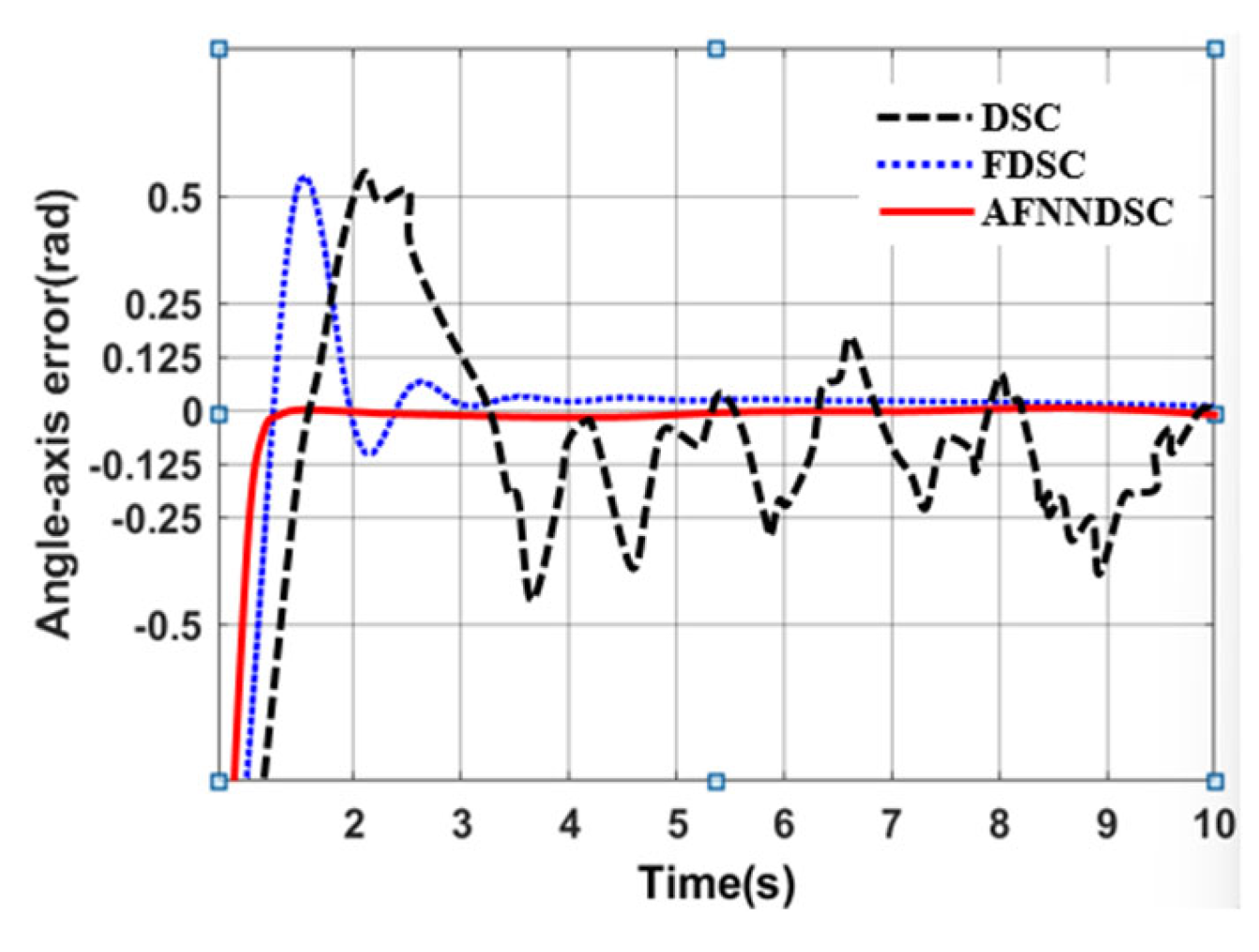
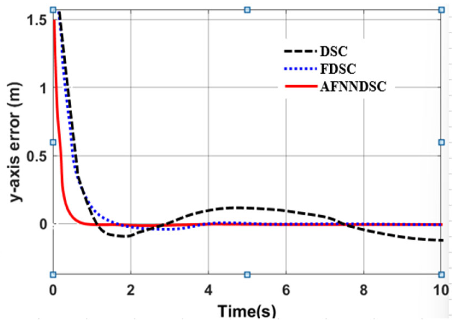
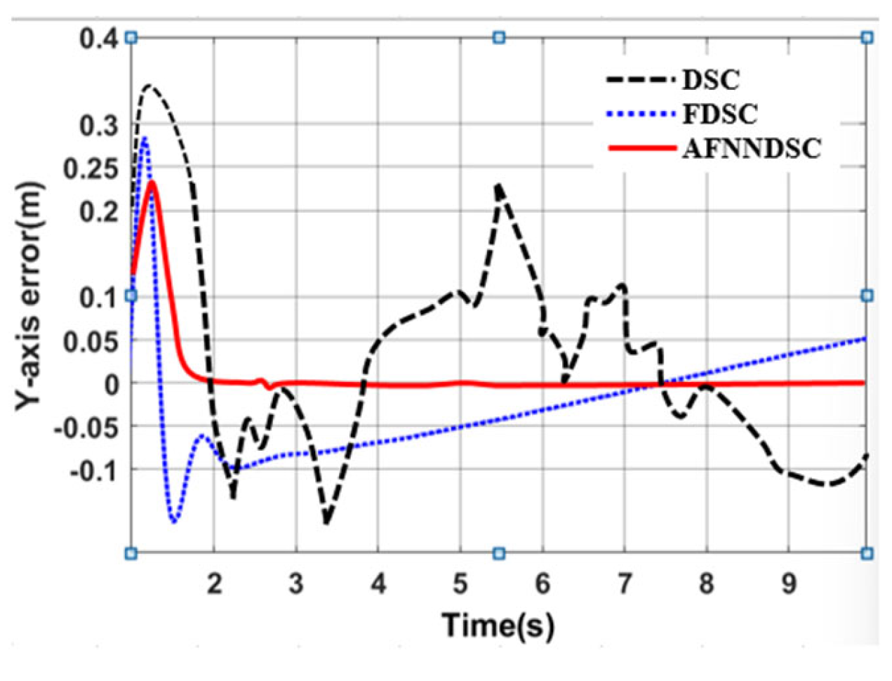
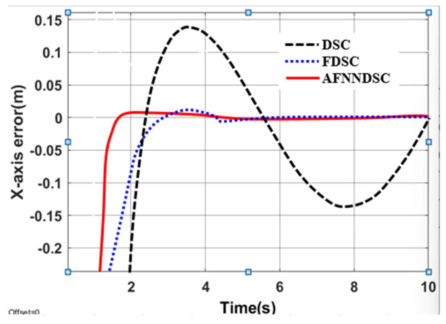
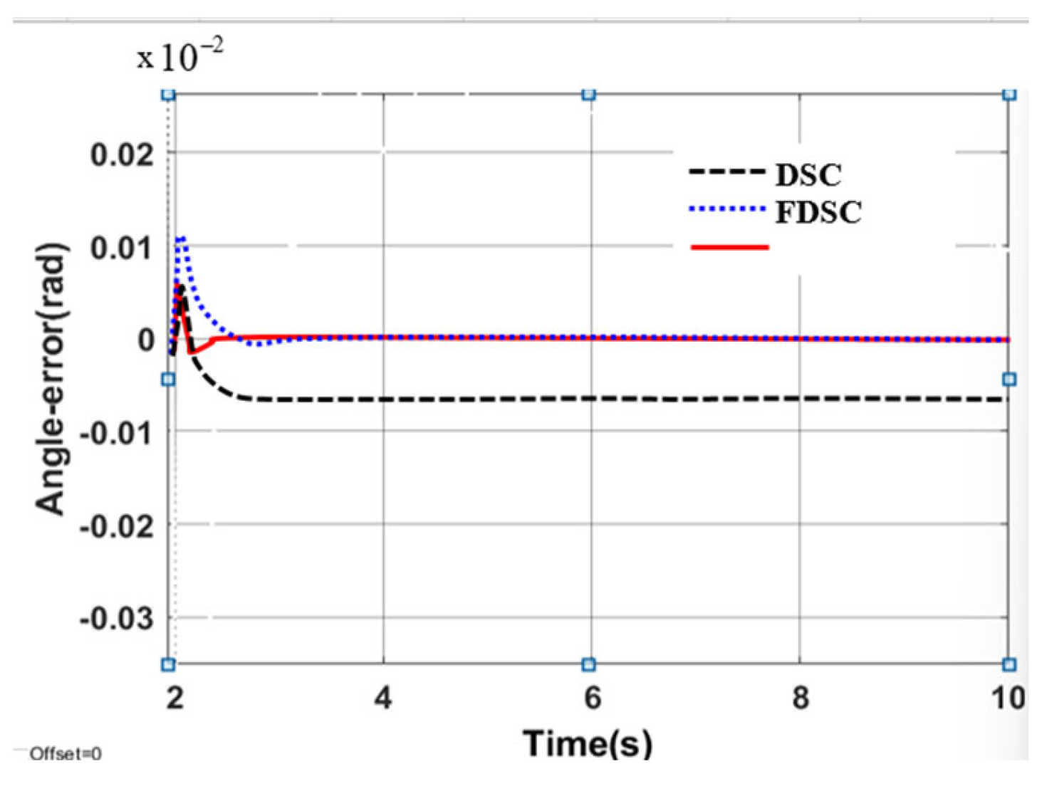
3.3.2. Result Simulation of Adaptive Fuzzy Neural Network Dynamic Surface Controller

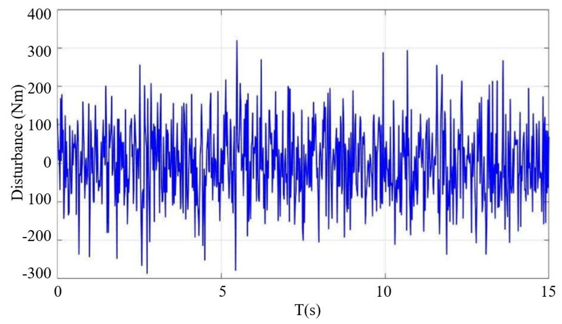
The Robot Model Is Affected by External Disturbances

In this case, the quality of the controller affecting the system is verified and evaluated under the condition that the robot’s motors are directly affected by external disturbance torques, namely Gauss noise, in which the interference is ignored. For the influence of friction, the coefficient of the selected sliding surface is: $\lambda =diag(10,10,10)$.

Conducting simulations and evaluating the proposed new algorithm with external noise (Figure 18) and circular orbit and a circular trajectory, the WMR will move from an initial point (0,0) inside the circle in the original coordinate system. The trajectory for the robot to follow according to the origin coordinate system is given by:$x=5\cos (\frac{\pi }{15}t);y=5\sin (\frac{\pi }{15}t); \theta =\frac{\pi }{15}t+\frac{\pi }{2}$.

From Figure 19, the AFNNDSC controller simulation structure is built on Matlab/Simulink.

Below are the simulation results. Figure 20, Figure 21 and Figure 22 compare the tracking errors in the WMR’s motion compared to a circular orbit when using DSC controllers, DSC controllers combined with fuzzy logic (AFDSC), respectively) and DSC controllers combined with a neural network and fuzzy logic system (AFNNDSC).

Comment: From Figure 20, Figure 21 and Figure 22, we can see that all three controllers can ensure the system’s tracking deviation compared to the set trajectory in the condition that the robot affected by external disturbance torques outside is not too large and is kept within an acceptable range. However, there is still a difference in quality between the controllers in the above results. When combining the DSC algorithm with the neural network and fuzzy logic system, the controller shows that the tracking quality is much better than the controller using the conventional DSC algorithm. It can be seen that, in conditions where robots are affected by uncertain external factors, conventional DSC controllers are not highly appreciated because it is difficult to determine the exact model of the robot due to the constant impact continuity of external disturbances. The AFNNDSC controller is a combination of a DSC, fuzzy logic system, and RBF neural network. In this case, the task will be to appropriately adjust the controller coefficients with fuzzy rules and approximate uncertain components in the robot model through the neural network, thereby improving the system’s response time as well as the deviation from the set trajectory. It can be clearly seen from the above simulation results when the time for the robot to approach the set value is about 0.2 s when using the AFNNDSC controller. Figure 23 and Figure 24 depict the change of control parameters when applying fuzzy rules.

The controller parameters are optimized based on fuzzy adaptive law to help the system state move faster to the sliding surface, the control parameters are continuously updated throughout the system’s movement. During the initial period when the robot has not yet approached the set trajectory, the robot’s tracking error is large, so the control parameters need to have large enough values to ensure that the system states quickly approach the sliding surface. Then, when approaching the set trajectory, the control parameters need to be adjusted to a smaller extent to avoid the “chattering” phenomenon on the sliding surface but still ensure that the robot sticks closely to the set trajectory.

Figure 25 depicts the movement of the WMR compared to the set trajectory when applying different control algorithms on two types of orbits. In general, the controllers ensure the ability to follow the robot’s trajectory. However, the adaptive controller AFNNDSC shows better performance than both other controllers in reducing the transient time as well as the error static deviation of the system.

Impact of Variation in Friction Coefficient from the Environment

One of the most common problems in controlling the movement of a WMR as well as mobile robots in general is the influence of the environment and especially the friction coefficient. In the robot kinematic model expression, friction coefficient values are often assumed in a fixed environment or ignored to facilitate algorithm design. However, in reality, these coefficients in the environment are a parameter that is difficult to determine accurately and change depending on the environment. Therefore, in this section, the simulation results assuming that the friction coefficient matrices $C(q,\dot{q})=diag(B_x,B_y,B_{\theta })$ and $G(q)=diag(C_x,C_y,C_{\theta })$ from the environment are variable coefficients cannot be determined accurately. Then, the neural network will predict and approximate the appropriate value of $\widehat{\mathrm{\Phi }}={[{\widehat{\mathrm{\Phi }}}_x,{\widehat{\mathrm{\Phi }}}_y,{\widehat{\mathrm{\Phi }}}_{\theta }]}^T$ to ensure the stability of the system as shown in Figure 26, Figure 27 and Figure 28. Uncertain values are approximated and converged by the neural network to an approximate value (approximately equal to the real value of the uncertainty value) and improve the control quality of the system.

In this case, the quality difference between controllers in reducing system deviations from the set trajectory can be clearly seen.

The tracking error of the system as well as the time for the system to reach the set orbit when using the DSC controller is the largest, while there is no significant difference between the two controllers FDSC and AFNNDSC in Figure 29, Figure 30 and Figure 31. Furthermore, with the change in the friction coefficient of the environment, the DSC controller cannot completely eliminate the deviation of the system.

Table 4. Maximum values of tracking errors when the robot moves according to set trajectories.

Controller	The Largest Deviation Value When the Robot Follows the Trajectory
	X-axis (m)	Y-axis (m)	Angle (rad)
DSC	0.1452	0.1683	0.00652
AFDSC	0.00136	0.00415	0.000452
AFNNDSC	0.000572	0.000523	0.000394

compares the tracking error of the system when applying three controllers in case the system is affected by environmental impacts.

Although the robot model is affected by environmental friction, all three controllers, the DSC controller, AFDSC controller, and AFNNDSC controller, can still ensure the ability to follow the robot’s trajectory. A new adaptive DSC for the WMR based on a fuzzy logic system and artificial neural network overcomes the chattering phenomenon due to the noise and jaw impact sign() of the DSC; AFDSC has been a suitable proposal to improve the tracking quality for a WMR in the case of model errors and slight amplitude impact noise. However, in case of large model deviations, the control quality is no longer guaranteed. Therefore, estimating model errors and compensating for the controller components will improve this controller’s quality. However, the AFNNDSC adaptive controller ensures the best quality for the system in reducing transient times and eliminating system deviations. Table 4 shows the most significant tracking error when using the DSC controller; the control errors are all kept within acceptable thresholds.

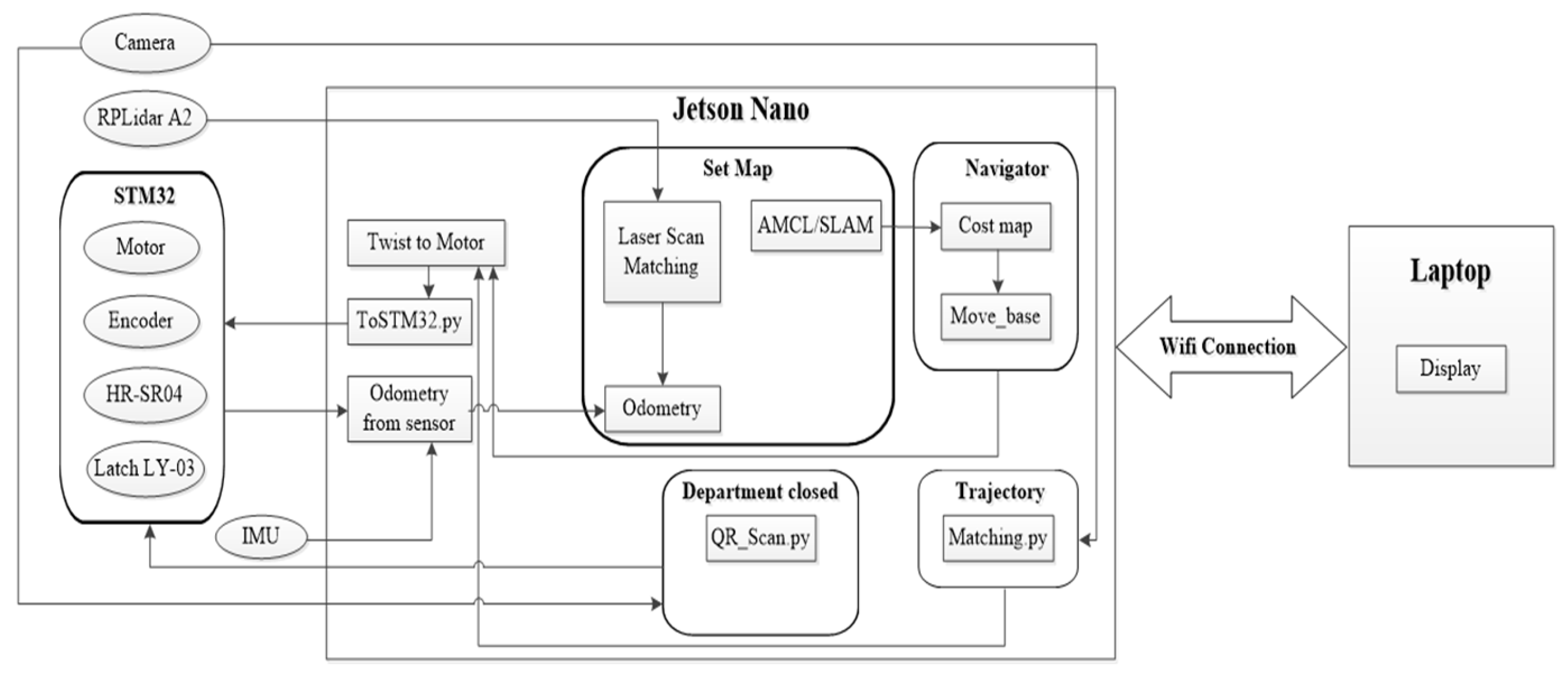
4. Fabrication and Experimental Operation of WMR with the Proposed Controller

4.1. Manufacturing WMR Model

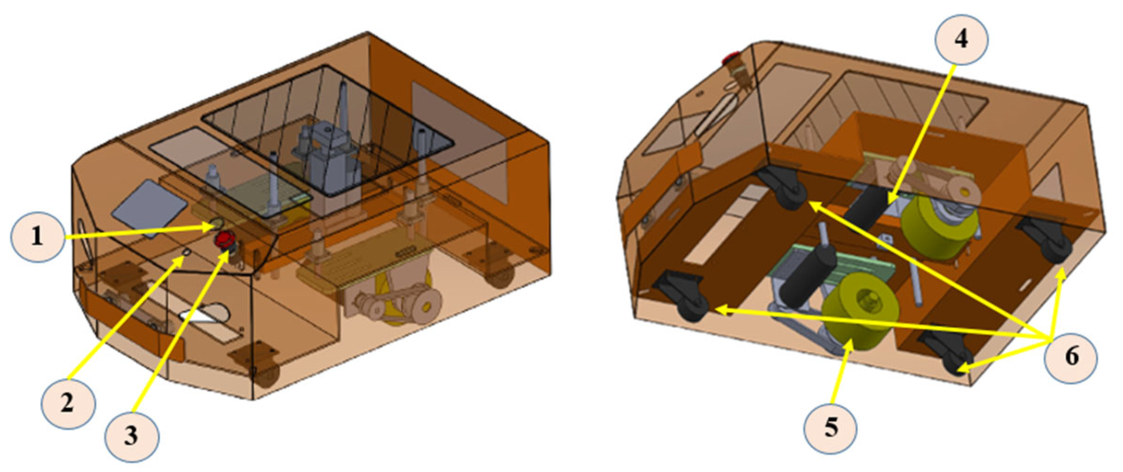
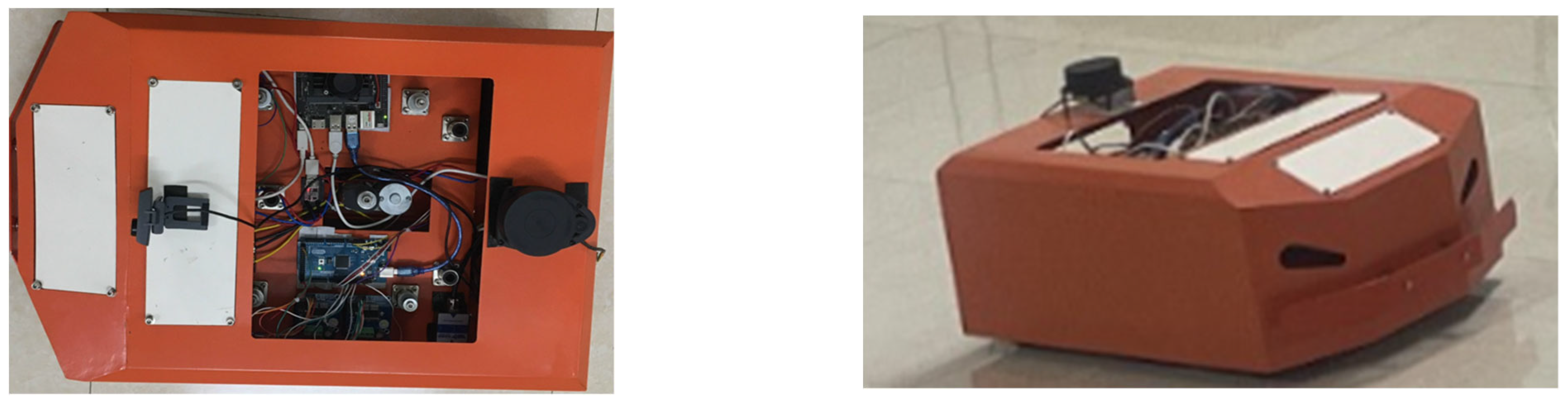
4.1.1. Mechanical Design of WMR

The WMR is built to specifications with a steel body measuring 75 × 62 × 38 cm (Figure 32 and Figure 33). Its 10-cm-diameter tires handle nearly any surface in the home. Four motor shafts hold 1200-tick encoders. This differential drive platform is comprehensive so it can rotate in place. The robot moves with two wheels. The robot is equipped with an ARM quad-core processor and 4 GB of RAM.

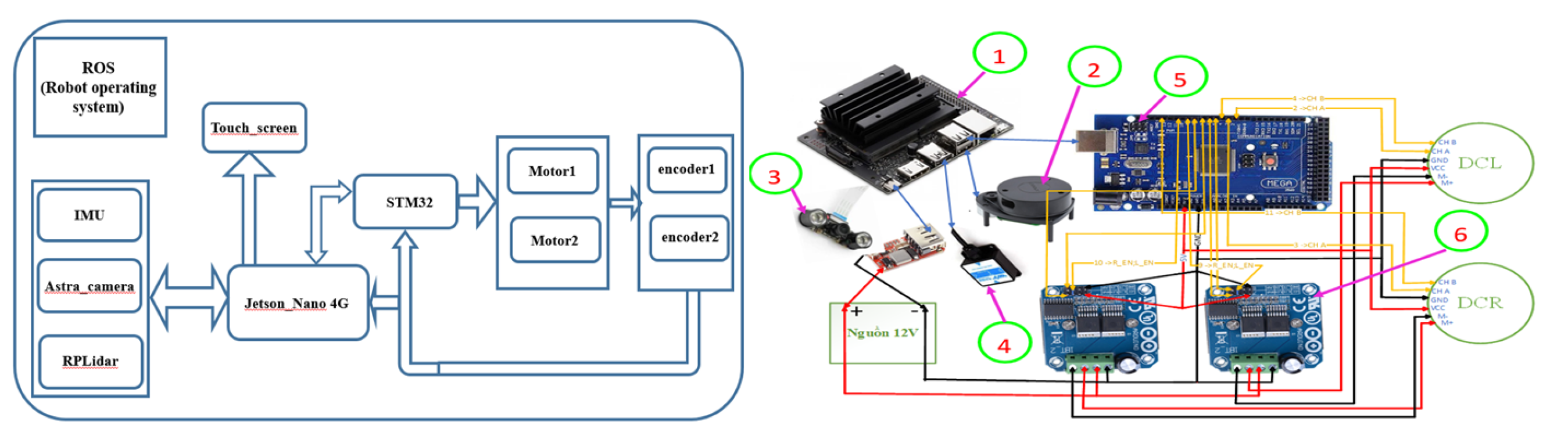
4.1.2. Design the Control Circuit Hardware Structure for the Robot

The control circuit hardware structure for the robot is used. A NVIDIA® Jetson Nano 4G (master) high-performance processor of country China, with the role of central processing, is a specialized high-performance processor for artificial intelligence processing. (WHO). The microcontroller circuit (slave) (uses ARM cortext M3 + DSP core, STM32F407VGT6, STMicroelectronics, China) is the part that receives control signals from the Jetson Nano 4G (master). The High-Power motor drive (BTS7960 43A: Large Current Motor Driver Module BTS7960 of Viet Nam) uses MOSFETs as the power circuit to control the four-wheel servo motors. The camera has an RGB image resolution of up to 1280 × 720. RPLIDAR A1M8 360° Lidar is a laser scanner, combined with the Astra 3D Camera that will send position, direction, and obstacle signals to the Jetson Nano master processor and sensor. The HWT901B IMU variable sends balanced signals to the Jetson master processor (Figure 34).

4.1.3. Robot Control Software

ROS programming software specifications, motor encoder information, and other I/O through packets from the Jetson Nano walker server all micro-control to the PC client and return control commands. The ROS2 Rolling with Focal (20.04) software provides library functions to handle navigation, path planning, obstacle avoidance, and many other robotic tasks (Figure 35).

Based on the powerful processing speed of the Jetson Nano 4G when processing neural networks that require large amounts of calculation and a fast processing speed, the robot programming platform operating system (ROS) is used because of its ability of optimal functionality for robot programming. Data from sensors, peripherals, and processing tasks are conveniently linked together using nodes. Each node is a programming program that performs a task, and the ROS provides a method of communication between these programs. Each node acts as a publisher (node used to export data) or subscriber (node used to receive data) or acts as both publisher and subscriber. Each exported data are named and called a “topic” in ROS, and these topics have names starting with a “/” and the name is placed after it. However, before being able to communicate with each other through topics, nodes must initially register first with “ros_master” as the node that plays the central role, storing the transmission and reception information of other nodes.

The control signal is calculated based on the ROS2 platform installed on the Jetson Nano embedded computer and then sent to the actuator control section installed on the embedded chip using STM32 (Figure 36).

Basically, the ROS has essential features of an operating system such as the ability to perform tasks in parallel, communicate and exchange data between tasks, data management, etc. An ROS can be used in the field of robotics. ROS is also developed specifically for libraries and tools for data collection, processing, control, etc. An ROS can interact with many other frameworks such as Player, YARP, Orocos, and Microsoft Robotics Studio.

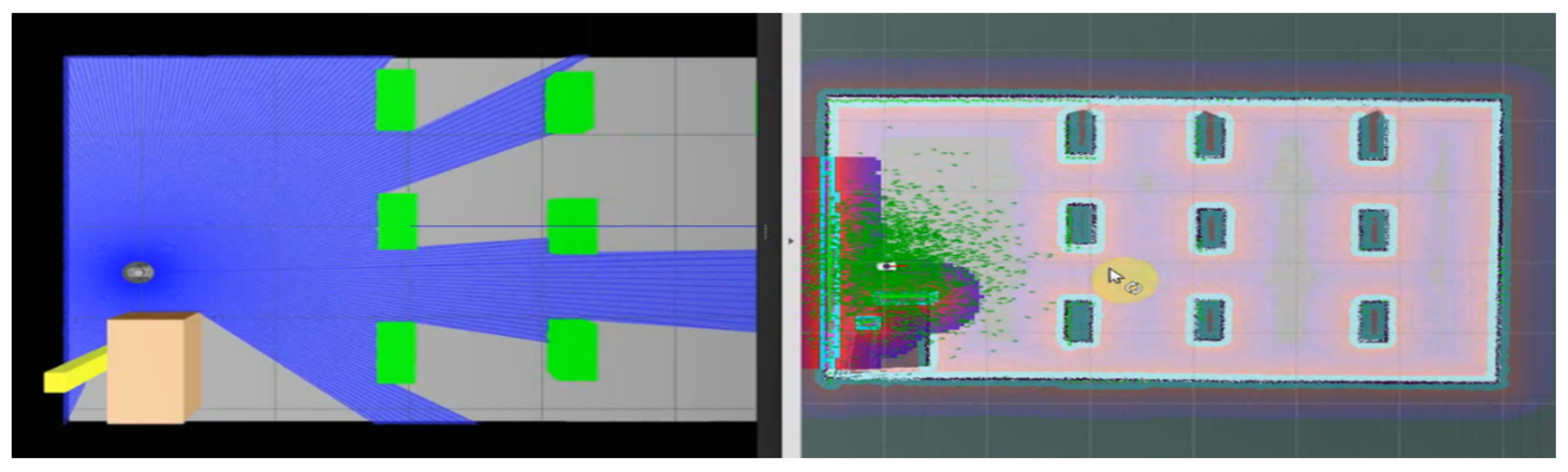
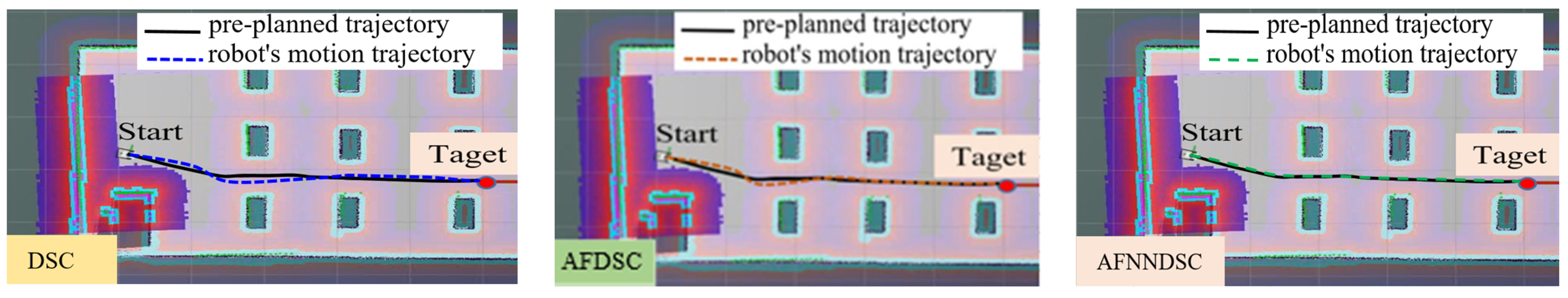
4.2. Simulate the Controller Tracking the Planned Trajectory on Gazebo

Figure 37 is a 3D model of the environment built using Gazebo ROS2 classic version 11 software to conduct algorithm testing in a simulated environment.

The motion response of the WMR with three controllers on the Gazebo is shown in Figure 38.

Figure 38 is the result of the robot’s motion trajectory obtained from Gazebo with the black line being the planned trajectory for the robot and in the established environment with the impact of the friction coefficient. It can be seen that the results when using the AFNNDSC algorithm to control the robot give clearly better results than the DSC and AFDSC controllers. With the aim of solving the challenges that come from the complexity of the software architecture of an autonomous vehicle and robot system, the robot operating system (ROS2) is an important platform that facilitates the development of these projects in this field. This is a framework responsible for synchronizing the robot’s software modules, abstracting hardware details for programmers, and ROS also provides simulation and visualization tools for robot models in the virtual environment, like Gazebo (Figure 37). Thanks to this, developers can conveniently carry out robotics projects in both the deployment and testing phases.

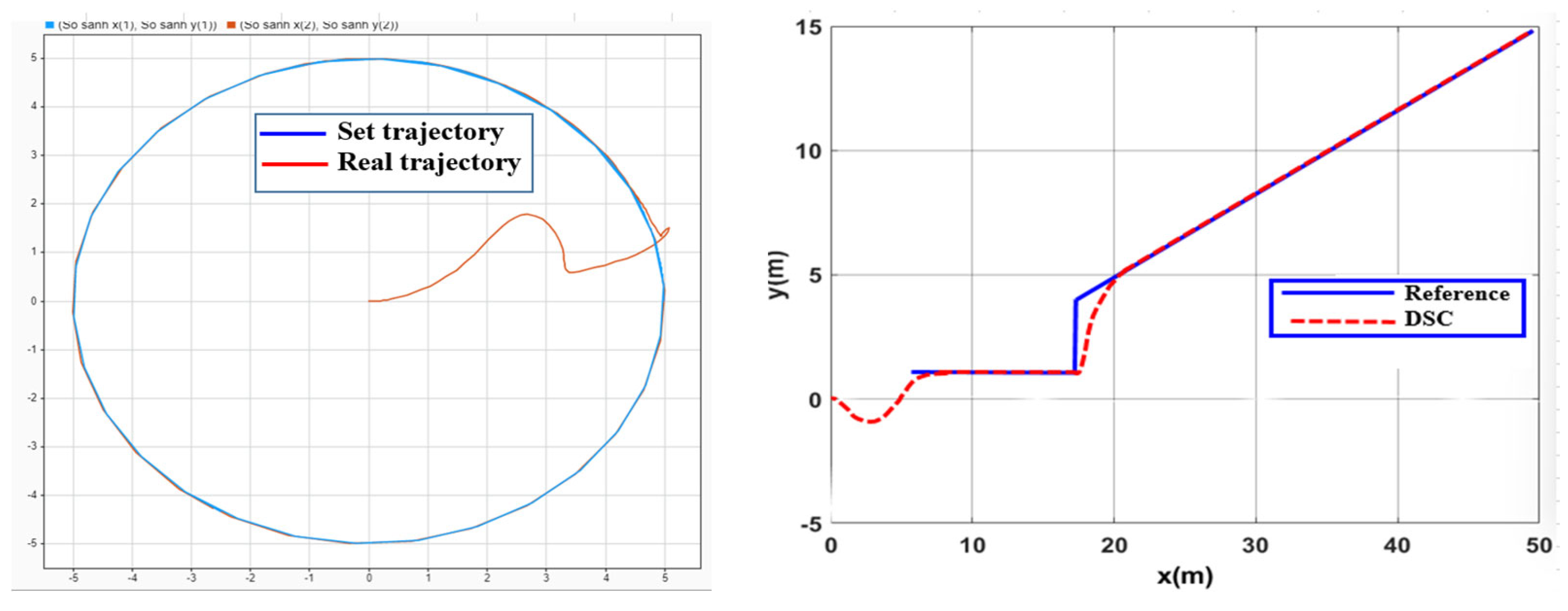
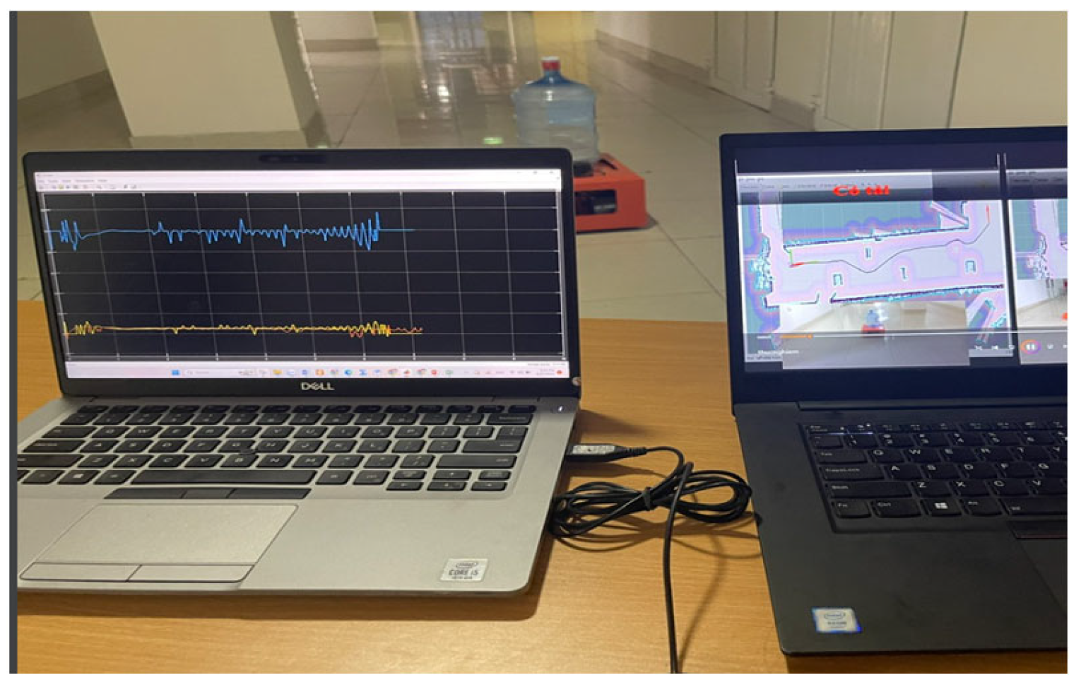
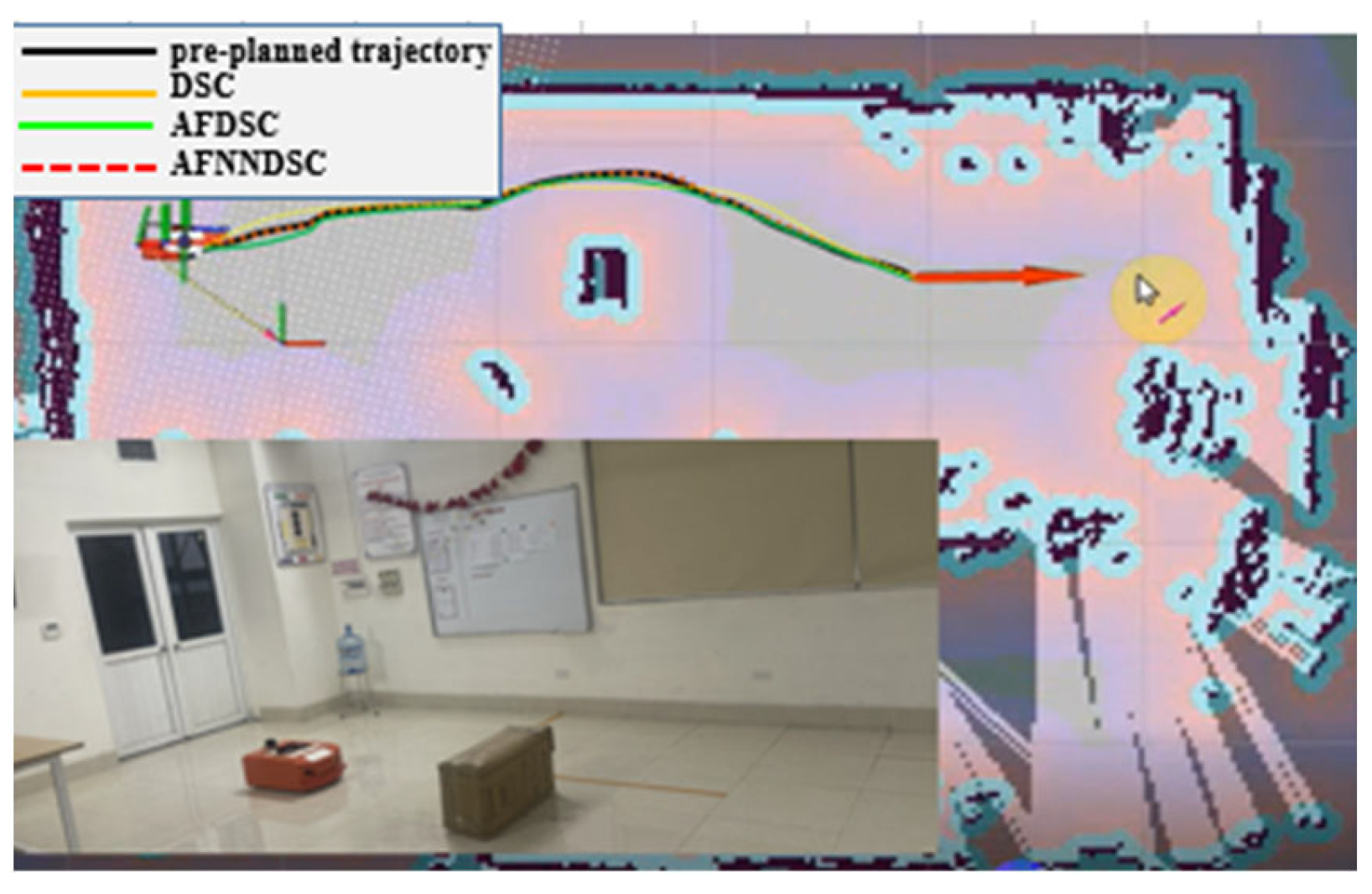
4.3. Experimental Model to Verify Results

Whelle mobile robot parameters when doing experiments are as follows: $\mathrm{m}=13 \mathrm{kg}; \mathrm{J}=0{.56 \mathrm{kg}/\mathrm{m}}^2,$ $r=0.08 \mathrm{m}; 2\mathrm{L}=0.6 \mathrm{m}$.

Test system structure: The A WMR with hardware: the computer contains a human–machine interface screen, Rviz (communicates with TX2 via WiFi) can observe the status and online position of the robot, and the HMI monitoring screen communicates via writing on Visual C (communicates with robot via RF) and can store and plot the real trajectory of the robot online. The robot’s position is set to the origin coordinates, and measured online through the IMU, calculated through four encoders, and a Lidar scanner. Any orbit can be set. The top of the laboratory’s ceiling is mounted with a camera to record the robot’s running process.

Test script: The WMR in the paper was tested in a laboratory environment.

Experiment: The robot was running in the background with many curves in the hallway (Figure 39) and the robot running in a room environment according to the surrounding area with polylines in the corners of the room as well as with three controllers, DSC, AFDSC, and AFNNDSC.

The experiments were conducted in two different environments, a hallway and a room. When giving the robot a destination, according to the D* pathfinding algorithm, the robot will plan a trajectory to avoid obstacles in the environment and reach the destination. When doing experiments, there will be two computer screens to control and monitor, one screen to see the map and actual path of the robot and one screen to see the controller’s response.

+Experiment with the robot running in an environment with many curves in the hallway (Figure 39).

The results of the experimental orbit in the corridor are displayed on Rvit as shown in Figure 40 when experimenting with three controllers, DSC, AFDSC, and AFNNDSC.

Case 2: Test the robot running in a room (environment according to the surrounding area with polylines in the corners of the room as well as with three controllers, DSC, AFDSC, and AFNNDSC as shown in Figure 41. The actual orbital response is displayed on Revit as shown in Figure 42.

Through the experiments, we can also see clear results of the optimal trajectory tracking of the AFNNDSC controller compared to the DSC and AFDSC controllers. When experimenting in two different environments, all three controllers responded well to the planned trajectory. However, for environments where the trajectory has many bends and turns, the trajectory tracking error is higher but not significant (

Table 5. Trajectory errors when running experiments with the proposed controllers.

${\mathit{N}}_{\mathit{o}}$	Experimental Environment	DSC Controller	AFDSC Controller	AFDSC Controller
1	Around the room	0.04163 (m)	0.00968 (m)	0.000934 (m)
2	Along the corridor	0.02431 (m)	0.007217 (m)	0.000763 (m)

). For the AFNNDSC controller, the error is only about 0.000934 (m) in the environ-ment around the room with many curves (Figure 41 and Figure 42) and 0.000763 (m) in the corridor environment (Figure 39 and Figure 40).

5. Conclusions

In this study, we have successfully built a kinematic and dynamic model of a mobile robot when there is side sliding. Kinematic and dynamic models all contain kinematics and dynamics of horizontal sliding. Then, we proposed an adaptive control law of an active fuzzy sliding surface for WMR orbital tracking based on an uncertain nonlinear system, paying particular attention to the tracking quality and the parameters change. The robot (because the application purpose of the robot is to interact with different objects and environments) is affected by noise when operating. The stability of the control law has been verified using Matlab-Simulink when conducting simulations for the robot to follow circular and square orbits. At the same time, the article’s content also presents the design, fabrication, and successful testing of the product WMR robot, which has hardware, a high-performance processing control circuit, and software to support programming on the operating system platform. The ROS2 robot gives experimental results that are consistent with theoretical analysis.

However, the vehicle is assumed to move on a flat surface with a limited load of 20 kg. The development direction of the article is to research and improve adaptive algorithms when robots move on a sloping terrain (3D) and have movement patterns suitable for different types of complex landscapes when operating practical applications with many other loads.

References

1. Hu, T.; Yang, S.; Wang, F.; Mittal, G. A neural network for a non-holonomic mobile robot with unknown robot parameters. In Proceedings of the 2002 IEEE International Conference on Robotics and Automation, ICRA 2002, Washington, DC, USA, 11–15 May 2002. [Google Scholar]
2. Hu, T.; Yang, S. A novel tracking control method for a wheeled mobile robot. In Proceedings of the 2nd Workshop on Computational Kinematics, Seoul, Republic of Korea, 20–22 May 2001; pp. 104–116. [Google Scholar]
3. Tiep, D.K.; Lee, K.; Im, D.-Y.; Kwak, B.; Ryoo, Y.-J. Design of Fuzzy-PID Controller for Path Tracking of Mobile Robot with Differential Drive. Int. J. Fuzzy Log. Intell. Syst. 2018, 18, 220–228. [Google Scholar] [CrossRef]
4. Souma, M.; Alia, A.; Hall, E.L. Designing and simulation a motion Controller for a Wheeled Mobile Robot Autonomous Navigation). In Proceedings of the SPIE Intelligent Robots and Computer Vision Conference, Sydney, Australia, 3–6 December 2013. [Google Scholar]
5. Zhao, L.; Wang, G.; Fan, X.; Li, Y. The Analysis of Trajectory Control of Non-holonomic Mobile Robots Based on Internet of Things Target Image Enhancement Technology and Backpropagation Neural Network. Front. Neurorobotics 2021, 15, 634340. [Google Scholar] [CrossRef]
6. Rubio, F.; Valero, F.; Llopis-Albert, C. A review of mobile robots: Concepts, methods, theoretical framework, and applications. Sage J. 2019, 10, 172988141983959. [Google Scholar] [CrossRef]
7. Wang, H.Y.; Wang, S. Trajectory Tracking Control for Nonholonomic Wheeled Mobile Robots with External Disturbances and Parameter Uncertainties. Int. J. Control Autom. Syst. 2020, 18, 3015–3022. [Google Scholar] [CrossRef]
8. Tinh, N.V.; Kiem, N.T.; Tuan Hung, D.; Pham, T. Neural Network-based Adaptive Sliding Mode Control Method for Tracking of a Nonholonomic Wheeled Mobile Robot with Unknown Wheel Slips, Model Uncertainties, and Unknown Bounded External Disturbances. Acta Polytech. Hung. 2018, 15, 103–123. [Google Scholar]
9. Liu, T.; Zhang, P.; Wang, M.; Jiang, Z.-P. New Results in Stabilization of Uncertain Nonholonomic Systems: An Event-Triggered Control Approach. J. Syst. Sci. Complex. 2021, 34, 1953–1972. [Google Scholar] [CrossRef]
10. Wang, X.F.; Wang, C. Robust Adaptive Terminal Sliding Mode Control of an Omnidirectional Mobile Robot for Aircraft Skin Inspection. Int. J. Control Autom. Syst. 2021, 19, 1078–1088. [Google Scholar]
11. Aldo, J.M.V.; Vicente, P.V.; Anand, S.O.; Juan, D.S.t. Adaptive Fuzzy Velocity Field Control for Navigation of Nonholonomic Mobile Robots. J. Intell. Robot. Syst. 2021, 101, 1–12. [Google Scholar]
12. Liu, Y.; He, W.; Qiao, H.; Ji, H. Adaptive-Neural-Network-Based Trajectory Tracking Control for a Nonholonomic Wheeled Mobile Robot with Velocity Constraints. IEEE Trans. Ind. Electron. 2021, 68, 5057–5067. [Google Scholar]
13. Zhang, J.-J.; Fang, Z.-L.; Zhang, Z.-Q.; Gao, R.-Z.; Zhang, S.-B. Trajectory Tracking Control of Nonholonomic Wheeled Mobile Robots Using Model Predictive Control Subjected to Lyapunov-Based Input Constraints. Int. J. Control Autom. Syst. 2022, 20, 1640–1651. [Google Scholar] [CrossRef]
14. Wang, S.; Bao, X.; Zhang, S.; Shen, G. Trajectory Tracking Control of Wheeled Mobile Robots Using Backstepping; Lecture Notes in Computer Science book series; Springer: Cham, Switzerland, 2019; Volume 11744, pp. 1393–1399. [Google Scholar]
15. Memon; Muhammad, J.R.; Attaullah, Y. Trajectory Tracking and Stabilization of Nonholonomic Wheeled Mobile Robot Using Recursive Integral Backstepping Control. Electronics 2021, 16, 1992. [Google Scholar]
16. Cui, M. Observer-Based Adaptive Tracking Control of Wheeled Mobile Robots with Unknown Slipping Parameters. IEEE Access 2019, 7, 169646–169655. [Google Scholar] [CrossRef]
17. Nourizadeh, P.; McFadden, F.J.S.; Browne, W.N. In situ slip estimation for mobile robots in outdoor environments. J. Field Robot. 2022, 40, 467–482. [Google Scholar] [CrossRef]
18. Liang, D.; Sun, N.; Wu, Y.; Fang, Y. Differential Flatness-Based Robust Control of Self-Balanced Robots. Int. J. Robot. Res. 2018, 51, 949–954. [Google Scholar] [CrossRef]
19. Ma, Z.; Liu, S.; Lyu, W.; Wang, K. Backstepping sliding mode-based anti-skid braking control for a civil aircraft. Aerosp. Syst. 2023, 6, 187–197. [Google Scholar] [CrossRef]
20. Sidek, N.; Sarkar, N. Dynamic modeling and control of nonholonomic mobile robot with lateral slip. In Proceedings of the 3rd International Conference on Systems, Cancun, Mexico, 13–18 April 2008; pp. 35–40. [Google Scholar]
21. Motte, I.; Campion, G.A. Slow manifold approach for the control of mobile robots not satisfying the kinematic constraints. IEEE Trans. Robot. Autom. 2010, 16, 875–880. [Google Scholar] [CrossRef]
22. Matveev, A.; Hoy, M.; Katupitiya, J.; Savkin, A. Nonlinear sliding mode control of an unmanned agricultural tractor in the presence of sliding and control saturation. Robot. Auton. Syst. 2013, 61, 973–987. [Google Scholar] [CrossRef]
23. Chen, C.; Gao, H.; Ding, L.; Li, W.; Yu, H.; Deng, Z. Trajectory tracking control of WMRs with lateral and longitudinal slippage based on active disturbance rejection control. Robot. Auton. Syst. 2018, 107, 236–245. [Google Scholar] [CrossRef]
24. Peña, C.; Cerqueira, J.J.F.; Lima, M.N. Control of wheeled mobile robots singularly perturbed by using the slipping and skidding variations: Curvilinear coordinates approach (Part I). IFAC-Papers-Online 2015, 48, 100–105. [Google Scholar] [CrossRef]
25. Sasiadek, J. Space Robotics and its Challenges. In GeoPlanet: Earth and Planetary Sciences; Springer: Berlin/Heidelberg, Germany, 2013; Volume 8, pp. 1–8. [Google Scholar] [CrossRef]
26. Cordo, A.T.; Nicolae, C. Evaluation of the Vehicle Sideslip Angle According to Different Road Conditions. In Proceedings of the 4th International Congress of Automotive and Transport Engineering, Cluj, Romania, 17–19 October 2018; pp. 814–819. [Google Scholar]
27. Zhang, L.; Chen, H.; Huang, Y.; Guo, H.; Sun, H.; Ding, H.; Wang, N. Model predictive control for integrated longitudinal and lateral stability of electric vehicles with in-wheel motors. Emerg. Trends LPV-Based Control Intell. Automot. Syst. 2020, 20, 1–19. [Google Scholar] [CrossRef]
28. Thiago, B.B.; Iossaqui, J.G.; Juan, F.C. Kinematic control design for wheeled mobile robots with longitudinal and lateral slip. arXiv 2021, arXiv:2105.06501. [Google Scholar]
29. Gao, X.; Yan, L.; Gerada, C. Modeling and Analysis in Trajectory Tracking Control for Wheeled Mobile Robots with Wheel Skidding and Slipping: Disturbance Rejection Perspective. Actuators 2021, 10, 222. [Google Scholar] [CrossRef]
30. Yoo, S. Approximation-based adaptive control for a class of mobile robots with unknown skidding and slipping. Int. J. Control Autom. Syst. 2012, 85, 703–710. [Google Scholar] [CrossRef]
31. Hoang, N.; Kang, H. Neural network-based adaptive tracking control of mobile robots in the presence of wheel slip and external disturbance force. Neurocomputing 2016, 188, 12–22. [Google Scholar] [CrossRef]
32. Low, C.B.; Wang, D. GPS-based tracking control for a car-like wheeled mobile robot with skidding and slipping. IEEE/ASME Trans. Mechatron. 2008, 13, 480–484. [Google Scholar]
33. Lenain, R.; Thuilot, B.; Cariou, C.; Martinet, P. Mixed kinematic and dynamic sideslip angle observer for accurate control of fast off-road mobile robots. J. Field Robot. 2010, 27, 181–196. [Google Scholar] [CrossRef]
34. Liu, J.; Wang, Z.; Zhang, L.; Walker, P. Sideslip angle estimation of ground vehicles: A comparative study. IET Control Theory Appl. 2021, 14, 3490–3505. [Google Scholar] [CrossRef]
35. Bayar, G.; Bergerman, M.; Konukseven, E.; Koku, A. Improving the trajectory tracking performance of autonomous orchard vehicles using wheel slip compensation. Biosyst. Eng. 2016, 146, 149–164. [Google Scholar] [CrossRef]
36. Grip, H.; Imsland, L.; Johansen, T.; Kalkkuhl, J.; Suissa, A. Vehicle sideslip estimation: Design, implementation and experimental validation. IEEE Control Syst. Mag. 2009, 29, 36–52. [Google Scholar]
37. Dakhlallah, J.; Glaser, S.; Mammar, S.; Sebsadji, Y. Tire-Road Forces Estimation Using Extended Kalman Filter and Sideslip Angle Evaluation. In Proceedings of the 2008 American Control Conference, Washington, DC, USA, 11–13 June 2008; pp. 4597–4602. [Google Scholar]
38. Fu, X.; Wang, S.; Yang, J.; Wang, Y.; Liu, Z. Adaptive Sliding Mode Control for Omnidirectional Mobile Robot Based on a New Friction Modeling. In Proceedings of the 2017 International Conference on Computer Technology, Electronics and Communication (ICCTEC), Dalian, China, 19–21 December 2017. [Google Scholar]
39. Swaroop, D.; Hedrick, J.K.; Yip, P.P.; Gerdes, J.C. Dynamic surface control for a class of nonlinearsystems. IEEE Trans. Automat. Contr. 2000, 45, 1893–1899. [Google Scholar] [CrossRef]
40. Tobergte, D.R.; Curtis, S. Dynamic Surface Control of Uncertain Nonlinear Systems; Springer: London, UK, 2013; Volume 53. [Google Scholar]
41. Edalati, L.; Khaki Sedigh, A.; Aliyari Shooredeli, M.; Moarefianpour, A. Adaptive fuzzy dynamic surface control of nonlinear systems with input saturation and time-varying output constraints. Mech. Syst. Signal Process. 2018, 100, 311–329. [Google Scholar] [CrossRef]
42. Gore, R.; Reynolds, P.F., Jr.; Kamensky, D.; Diallo, S.; Padilla, J. Statistical debugging for simulations. ACM Trans. Model. Comput. Simul. (TOMACS) 2015, 25, 1–26. [Google Scholar] [CrossRef]
43. Qi, S.; Zhang, D.; Guo, L.; Wu, L. Adaptive Dynamic Surface Control of Nonlinear Switched Systems with Prescribed Performance. J. Dyn. Control Syst. 2018, 24, 269–286. [Google Scholar] [CrossRef]
44. Wang, C.; Wang, D.; Han, Y. Neural Network Based Adaptive Dynamic Surface Control for Omnidirectional Mobile Robots Tracking Control with Full-State Constraints and Input Saturation. Int. J. Control Autom. Syst. 2021, 19, s4067–s4077. [Google Scholar] [CrossRef]
45. Qin, P.; Zhao, T.; Liu, N.; Mei, Z.; Yan, W. Predefined-Time Fuzzy Neural Network Control for Omnidirectional Mobile Robot. Processes 2022, 11, 23. [Google Scholar] [CrossRef]
46. Huang, S.N.; Tan, K.K.; Lee, T.H. Adaptive motion control using neural network approximations. Automatica 2002, 38, 227–233. [Google Scholar] [CrossRef]
47. Xu, J.; Zhang, M.; Zhang, J. Kinematic model identification of autonomous Mobile Robot using dynamical recurrent neural networks. In Proceedings of the 2005 IEEE International Conference Mechatronics and Automation, Niagara Falls, ON, Canada, 29 July 2005–1 August 2005; Volume 3, pp. 1447–1450. [Google Scholar]
48. Ge, S.S.; Wang, C. Direct adaptive neural network control of a class of nonlinear systems. IEEE Trans. Neural Netw. 2002, 13, 214–221. [Google Scholar] [CrossRef]
49. Wang, J.; Chen, J.; Ouyang, S.; Yang, Y. Trajectory tracking control based on adaptive neural dynamics for four-wheel drive Omnidirectional mobile robots. Eng. Rev. 2014, 34, 235–243. [Google Scholar]
50. Yu, L.; Fei, S.; Yang, G. A Nơ ron Network Approach for Tracking Control of Uncertain Switched Nonlinear Systems with Unknown Dead-Zone Input. Circuits Syst. Signal Process 2015, 34, 2695–2710. [Google Scholar] [CrossRef]
51. Rosillo, N.; Montés, N.; Ferreira, N. A Generalized Matlab/ROS/Robotic Platform Framework for Teaching Robotics. Robot. Educ. 2019, 25, 159–169. [Google Scholar]
52. Araújo, A.; Portugal, D.; Couceiro, M.S.; Rocha, R.P. Integrating Arduino-Based Educational Mobile Robots in ROS. J. Intell. Robot. Syst. 2017, 77. [Google Scholar]
53. Rajesh, K.M.; Chint, R.T.; Sarath, S.; Akhil, R. ROS based Autonomous Indoor Navigation Simulation Using SLAM Algorithm. Int. J. Pure Appl. Math. 2018, 7, 199–205. [Google Scholar]
54. Yoshida, H.; Fujimoto, H.; Kawano, D.; Goto, Y.; Tsuchimoto, M.; Sato, K. ROS: An open-source Robot Operating System. In Proceedings of the 41st Annual Conference of the IEEE Industrial Electronics Society, Yokohama, Japan, 9–12 November 2015; pp. 4754–4759. [Google Scholar]
Figure 1. Wheeled mobile robot with horizontal sliding.
Actuators 13 00031 g001
Figure 2. Control system simulation structure using DSC controller.
Actuators 13 00031 g002
Figure 3. DSC controller simulation structure.
Actuators 13 00031 g003
Figure 4. Tracking trajectory and tracking error when using DSC with circular orbit.
Actuators 13 00031 g004
Figure 5. Tracking trajectory and tracking error when using DSC with a curved trajectory.
Actuators 13 00031 g005
Figure 6. Trajectory tracking when using DSC with noisy fields with circular and curved orbits.
Actuators 13 00031 g006
Figure 7. Structure of fuzzy adaptive dynamic sliding surface control system for WMR.
Actuators 13 00031 g007
Figure 8. Fuzzy sets for input e 1 .
Actuators 13 00031 g008
Figure 9. Fuzzy sets for input e ˙ 1 .
Actuators 13 00031 g009
Figure 10. External interference.
Actuators 13 00031 g010
Figure 11. Tracking trajectory and tracking error when using DSC and AFDSC controllers with noisy fields.
Actuators 13 00031 g011
Figure 12. Parameters c 1 .
Actuators 13 00031 g012
Figure 13. Parameters c 2 .
Actuators 13 00031 g013
Figure 14. Parameters c 3 .
Actuators 13 00031 g014
Figure 15. Motion of WMR with circular trajectory and folded trajectory.
Actuators 13 00031 g015
Figure 16. Controller structure diagram AFNNDSC.
Actuators 13 00031 g016
Figure 17. Radial neural network.
Actuators 13 00031 g017
Figure 18. Torque noise (Nm).
Actuators 13 00031 g018
Figure 19. Simulation structure of AFNNDSC controller on Matlab/Simulink.
Actuators 13 00031 g019
Figure 20. Error on x-axis.
Actuators 13 00031 g020
Figure 21. Error on y-axis.
Actuators 13 00031 g021
Figure 22. Angle error.
Actuators 13 00031 g022
Figure 23. Optimizing control parameters c 1 .
Actuators 13 00031 g023
Figure 24. Optimizing control parameters c 2 ( c 3 ) .
Actuators 13 00031 g024
Figure 25. Circular orbit and curved orbit with three controllers DSC, AFDSC, and AFNNDSC in case of external interference.
Actuators 13 00031 g025
Figure 26. The value of δ ^ x compared to δ x .
Actuators 13 00031 g026
Figure 27. The value of δ ^ y compared δ y .
Actuators 13 00031 g027
Figure 28. The value of δ ^ θ compared δ θ .
Actuators 13 00031 g028
Figure 29. Error on x-axis.
Actuators 13 00031 g029
Figure 30. Error on y-axis.
Actuators 13 00031 g030
Figure 31. Angle error.
Actuators 13 00031 g031
Figure 32. Mechanical design of wheeled mobile robot. 1. Switch On/Off; 2. Sirens; 3. Emergency stop button; 4. DC; 5. Active wheel; 6. Passive wheel.
Actuators 13 00031 g032
Figure 33. Building a realistic model.
Actuators 13 00031 g033
Figure 34. Structure diagram of the control hardware for the robot. 1: Jetson Nano 4GPlease state the name of the manufacturer, city, and country from where the equipment was sourced. 2: Lidar RPLIDAR A1M8 360°. 3: Camera AI. 4: IMU HWT901B. 5: STM32 F407. 6: Driver DC BTS7960 43A.
Actuators 13 00031 g034
Figure 35. Control software structure.
Actuators 13 00031 g035
Figure 36. Control software structure.
Actuators 13 00031 g036
Figure 37. Simulation of factory diagram on Gazebo and on Rvit.
Actuators 13 00031 g037
Figure 38. Trajectory planning for the robot.
Actuators 13 00031 g038
Figure 39. Experimental running of the WMR model in the hallway.
Actuators 13 00031 g039
Figure 40. WMR trajectory response when running in the corridor.
Actuators 13 00031 g040
Figure 41. Running the experimental model around the room.
Actuators 13 00031 g041
Figure 42. Orbital response of WMR when running experimentally around the room.
Actuators 13 00031 g042