An Accurate Dynamic Model Identification Method of an Industrial Robot Based on Double-Encoder Compensation

Abstract

Aiming at the challenges to accurately simulate complex friction models, link dynamics, and part uncertainty for high-precision robot-based manufacturing considering mechanical deformation and resonance, this study proposes a high-precision dynamic identification method with a double encoder. Considering the influence of the dynamic model of the manipulator on its control accuracy, a three-iterative global parameter identification method based on the least square method and GMM (Gaussian Mixture Model) under the optimized excitation trajectory is proposed. Firstly, a bidirectional friction model is constructed to avoid using residual torque to reduce the identification accuracy. Secondly, the condition number of the block regression matrix is used as the optimization objective. Finally, the joint torque is theoretically identified with the weighted least squares method. A nonlinear model distinguishing between high and low speeds was established to fit the nonlinear friction of the robot. By converting the position and velocity of the motor-side encoder to the linkage side using the deceleration ratio, the deformation quantity could be calculated based on the discrepancy between theoretical and actual values. The GMM algorithm is used to compensate the uncertainty torque that was caused by model inaccuracy. The effectiveness of the proposed method is verified by a simulation and experiment on a 6-DoF industrial robot. Results prove that the proposed method can enhance the online torque estimation performance by up to 20%.

1. Introduction

Traditional industrial robots are widely used in manufacturing due to their high speed and precision, such as in welding, spraying, polishing, and cutting, where stable processing trajectories are required. The performance of these tasks highly depends on accurate dynamic models, which must account for factors such as friction and unknown disturbance torques. Although the robot dynamics model can be obtained from CAD models, the parameters obtained through this method may not accurately reflect the actual dynamic parameters. Consequently, researchers have proposed various methods to decompose and analyze the robot dynamics model to improve its accuracy. Vandanjon [1] used a method that independently considers each part of the robot dynamics, identifies the inertial forces, centrifugal forces, inertial integrals, and gravity separately, and designs various exciting trajectories. While this method can enhance the model’s accuracy, excessive subdivisions will augment the model’s uncertainty and diminish the accuracy of the identification outcomes. Currently, the widely used method for robot model identification is the global identification method [2], which can comprehensively incorporate various factors in the dynamic modeling process, and collect and process data for all joints, before applying identification algorithms to calculate all dynamic parameters simultaneously. Due to its easy implementation, this has become a commonly practiced approach to robot dynamics modeling. The mainstream process is to determine the minimum identifiable parameter set and regression matrix [3]; on this basis, design the optimal exciting trajectory to fully stimulate the dynamic characteristics of the robot [4]. Solving for kinetic parameters, design the parameter identification algorithm through the data collected along the exciting trajectory. Designing the optimal exciting trajectory [5] and parameter identification algorithm is a current research hotspot. In the case of industrial robots lacking joint torque sensors, conventional identification methods [6,7,8] typically leverage proprioceptive signals, such as kinematic states and motor current. Direct access to the torques applied to the robot links is unavailable, as these values are affected by errors in friction modeling and the limited precision of torque constants. Consequently, the identification results are susceptible to disturbances. Identification methods based on current measurements depend on precise prior knowledge of joint drive gains [9]. Unfortunately, the calibration scenarios for drive gains provided by manufacturers often differ from the identification scenarios [10].

Because of the high-load joint rigidity of industrial robots, the theoretical modeling of dynamics is sufficient to approximate the real joint driving torque due to the separation design of driving and joints. However, small industrial manipulators have lightweight structures and components, such as harmonic reducers, double encoders, and torque sensors, resulting in a highly integrated servo drive and motor in a single joint. This structure reduces the rigidity of the joint. Thus, theoretical dynamics modeling can only establish the link dynamics on the load side, and the motor-side dynamics need to compensate for the flexible error. In order to address the challenges posed by flexible systems, robots often rely on torque sensors, as exemplified in study [11]. The introduction of joint torque sensors transforms the system into a passive control configuration, ensuring system stability. However, traditional industrial robots typically lack joint torque sensors, necessitating the use of flexible deformation from dual encoders for approximate torque compensation. The primary application scenario for this approach is dynamic identification, aiming to acquire more accurate models. This, in turn, facilitates applications such as drag teaching or collision detection. Spong [12] introduced a modeling approach for the flexible joints of the manipulator, equivalent to a spring model with only stiffness and damping between the motor end and the connecting-rod load end. However, because of the large stiffness of the operating arm, unless correspondingly large external forces are acting on the connecting rod, the error of the double encoder cannot fully capture the physical characteristics of the flexible joint. Therefore, researchers have proposed methods to improve the model, such as static parameter identification and neural network model fitting [13].

Linear identification methods typically model frictional forces as Coulomb and linear viscous forces. Coulomb and linear viscous forces are directly identified through the method discussed in [14]. However, some studies demonstrate a nonlinear relationship between the viscous frictional force and joint velocity [15,16]. Several identification methods have been widely used, including the least squares method [17], the weighted least squares method [18], and the maximum likelihood method [19]. The least squares method is a classic algorithm used in a linear regression analysis that is easy to understand and implement; however, it is vulnerable to noise and has poor robustness. For this reason, many scholars at home and abroad have conducted further research [20,21,22,23,24]. Recently, some researchers have utilized neural networks to establish dynamic models, but the results are unreliable due to the networks’ high sensitivity to noise and tendency to overfit. Thus, despite advancements in dynamic modeling, improving dynamic model accuracy is still an active area of research [25].

The motor and the load are not directly coupled but are essentially an elastic system. This paper presents an algorithm for the identification and compensation of dynamic model parameters for industrial robots, based on compensating for information with double encoders. This approach is exemplified using a 6-DOF industrial robot, where the minimum parameter set is derived by constructing the dynamic model and employing QR decomposition. The optimization parameters for the incentive trajectory are determined using a trajectory optimization algorithm, resulting in the acquisition of the optimized incentive trajectory. Subsequently, upon obtaining the trajectory, joint torque is identified using the iterative weighted least squares method. The nonlinear friction force of the manipulator is modeled by constructing a nonlinear model that distinguishes between high and low speeds. The WLS (weighted least squares) method is used for the identification of the dynamic parameters. Finally, the information of the nonlinear residue is fitted using a double encoder to complete the identification and compensation of dynamic parameters of the industrial manipulator. To address uncertainties in torque components that cannot be precisely modeled, the GMM (Gaussian Mixture Model) algorithm is applied for compensation. This improves the accuracy and robustness of the identification results. The entire dynamic identification process in this study is conducted in an offline mode, with only torque estimation being performed in real-time online. Figure 1 illustrates the functional flowchart of the offline identification method.

The rest of the article is arranged as follows: Section 2 introduces the linearization of the dynamic model and the identification of friction. Section 3 proposes the block regression matrix, which is used as the index to optimize the trajectory parameters for obtaining a relatively ideal exciting trajectory. Section 4 provides the identification method of the dynamic parameters based on WLS. Section 5 proposes the GMM algorithm, which is used to compensate for the uncertain torque component that cannot be accurately modeled. The simulation and experimental results are demonstrated in Section 6. At last, Section 7 concludes the article.

2. Linearization of Dynamic Model and Identification of Friction

The expression of the joint torques of a serial robot can be obtained using the Newton–Euler iterative method base on MDH [26] and can be represented as follows: “∈”.

$${\mathit{\tau }}_m=\mathit{M}(\mathit{\theta })\ddot{\mathit{\theta }}+\mathit{C}(\mathit{\theta },\dot{\mathit{\theta }})+\mathit{G}(\mathit{\theta })+{\mathit{\tau }}_f+\mathit{J}{(\mathit{\theta })}^{\mathrm{T}}{\mathit{F}}_{ext}+{\mathit{\tau }}_u$$

(1)

In this equation, $\mathit{M}\left(\mathit{\theta }\right)\in {\mathbb{R}}^{n\times n}$ and $n$ represent the positive definite symmetric inertia matrix and the number of joints, respectively. $\mathit{C}\left(\mathit{\theta },\dot{\mathit{\theta }}\right)\in {\mathbb{R}}^{n\times n}$ and $\mathit{G}\left(\mathit{\theta }\right)\in {\mathbb{R}}^{n\times 1}$ represent the Coriolis and gravitational torques, respectively. $\mathit{\theta }$,$\dot{\mathit{\theta }},\ddot{\mathit{\theta }}$ are displacement, velocity, and acceleration vectors of the joint’s $n\times 1$ vector space. ${\mathit{\tau }}_m\in {\mathbb{R}}^{n\times 1}$ and ${\mathit{\tau }}_f\in {\mathbb{R}}^{n\times 1}$ represent the driving torque and frictional torque of the joint in the dynamic model, respectively. ${\mathit{F}}_{\mathrm{ext}}$ and $\mathit{J}\left(\mathit{\theta }\right)$ represent the external force acting on the robot endpoint and jacobian matrix, and ${\mathit{\tau }}_u\in {\mathbb{R}}^{n\times 1}$ represents the unmodeled and disturbance torques of the joint. Since the external force, unmodeled part, and disturbance torque are independent of the parameters of the robot dynamic model itself, the dynamic model becomes a link dynamic model. Therefore, in this paper, Equation (1) is linearized [3] to obtain the link dynamic model. The link dynamic model is built solely on the characteristics of the link, without accounting for joint influences. On the other hand, the joint dynamic model incorporates the effects of joint parameters. The torque in this part will be studied in the following text. After rearranging the link dynamic parameters of the robot to be identified and removing and integrating the columns that do not affect the identification process, the basic dynamic parameters, namely the minimum parameters, will be obtained.

$${\mathit{\tau }}_{link}=\left[\begin{array}{ll}{\mathit{\Gamma }}_{link}\hfill & {\mathit{\Gamma }}_f\hfill \end{array}\right]\left[\begin{array}{c}{\mathit{\Phi }}_{link}\\ {\mathit{\Phi }}_f\end{array}\right]=\mathit{\Gamma }\mathit{\Phi }$$

(2)

The dynamic model becomes a dynamic model of a link without a motor. Where ${\mathit{\tau }}_{link}\in {\mathbb{R}}^{n\times 1}$ is link torque, ${\mathit{\Gamma }}_{link}\in {\mathbb{R}}^{n\times rank\left({\mathit{\Gamma }}_{link}\right)}$ is link parameters, ${\mathit{\Phi }}_{link}\in {\mathbb{R}}^{rank\left({\mathit{\Gamma }}_{link}\right)\times 1}$ is the link regression matrix, ${\mathit{\Gamma }}_f\in {\mathbb{R}}^{n\times 8}$ is friction parameters, and ${\mathit{\Phi }}_f\in {\mathbb{R}}^{8\times 1}$ is the friction regression matrix. $\mathit{\Gamma }$ is solely dependent on the mechanical arm’s motion state and independent of its structural parameters. The regression matrix can be obtained using the kinematic formula. $\mathit{\Phi }$ represents the minimum set of expressions corresponding to the dynamic structural parameters. Bidirectional torque detection is an accurate method to obtain frictional force data. It can be derived that the Coriolis/centrifugal matrix satisfies

$$\mathit{C}(\mathit{\theta },-\dot{\mathit{\theta }})(-\dot{\mathit{\theta }})=\mathit{C}(\mathit{\theta },\dot{\mathit{\theta }})\dot{\mathit{\theta }}$$

(3)

Given that a majority of industrial robots lack joint torque sensors, directly acquiring joint friction torque becomes impractical. Nevertheless, it is feasible to deduce the joint friction torque by examining the characteristics and design of the robot’s configuration and kinematic state. Industrial robots typically feature encoders on each joint’s motors, enabling the direct reading of joint velocity. Subsequently, [27] introduces a bidirectional friction estimation method for extracting joint friction torque from the overall joint torques. For simplicity, it can be assumed that the friction torque is only related to the joint velocity:

$${\mathit{\tau }}_f(-\dot{\mathit{\theta }})=-{\mathit{\tau }}_f(\dot{\mathit{\theta }})$$

(4)

Assume two industrial robot configurations ${\mathit{\theta }}_1$, ${\mathit{\theta }}_2$ meet the following conditions:

$$\begin{array}{c}{\mathit{\theta }}_1={\mathit{\theta }}_2=\mathit{q}\\ {\dot{\mathit{\theta }}}_1=-{\dot{\mathit{\theta }}}_2=\dot{\mathit{q}}\\ {\ddot{\mathit{\theta }}}_1=-{\ddot{\mathit{\theta }}}_2=\ddot{\mathit{q}}\end{array}$$

(5)

Substituting Equation (5) into Equation (3), it can be obtained that

$$\begin{array}{l}{\mathit{\tau }}_1=\mathit{M}(\mathit{q})\ddot{\mathit{q}}+\mathit{C}(\mathit{q},\dot{\mathit{q}})\dot{\mathit{q}}+\mathit{G}(\mathit{q})+{\mathit{\tau }}_{estf}(\dot{\mathit{\theta }})\\ {\mathit{\tau }}_2=\mathit{M}(\mathit{q})(-\ddot{\mathit{q}})+\mathit{C}(\mathit{q},-\dot{\mathit{q}})(-\dot{\mathit{q}})+\mathit{G}(\mathit{q})+{\mathit{\tau }}_{estf}(-\dot{\mathit{\theta }})\end{array}$$

(6)

Substituting Equation (5) into Equation (6), it can be found that

$${\mathit{\tau }}_1-{\mathit{\tau }}_2=2\mathit{M}(\mathit{q})\ddot{\mathit{q}}+2{\mathit{\tau }}_{estf}(\dot{\mathit{q}})$$

(7)

According to Equation (7), when the robot moves slowly, friction is typically obtained under low-speed and constant-speed conditions, where joint accelerations are exceedingly small and can be approximated as negligible. This method provides a straightforward and easily implementable approach for acquiring frictional force data in robotic arm systems. The inertia force/torque $\mathit{M}\left(\mathit{q}\right)$ can be ignored, and it can be obtained that

$${\mathit{\tau }}_{estf}(\dot{\theta })=\frac{{\mathit{\tau }}_1-{\mathit{\tau }}_2}{2}$$

(8)

A common approach for dynamic model identification involves assuming the friction model as Coulomb friction plus viscous friction linear to the joint velocity; this is often inadequate in practical scenarios. Recognizing the nonlinearity of friction, several advanced friction models have been proposed in relevant literature [28,29]. However, these models are typically isolated from mass-inertial parameters and identified independently using nonlinear optimization methods. In recent developments, a unified approach has been introduced for dynamic model identification that incorporates nonlinear friction. This paper adopts the following nonlinear friction model for each joint:

$${\tau }_{fi}=\{\begin{array}{c}\begin{array}{cc}{\tau }_{fci}& \left|{\dot{\theta }}_i\right|<\lambda \end{array}\\ \begin{array}{cc}{\tau }_{fci}+{\tau }_{fvi}& \left|{\dot{\theta }}_i\right|\ge \lambda \end{array}\end{array}$$

(9)

$${\tau }_{fci}=\{\begin{array}{ll}{k}_{ci1}\frac{\tanh \left(\frac{{\dot{\theta }}_i}{eps}\right)\left(\tanh \left(\frac{{\dot{\theta }}_i}{eps}\right)+1\right)}{2}\hfill & {\dot{\theta }}_i\ge 0\hfill \\ k_{ci2}\frac{\tanh \left(\frac{{\dot{\theta }}_i}{eps}\right)\left(1-\tanh \left(\frac{{\dot{\theta }}_i}{eps}\right)\right)}{2}\hfill & {\dot{\theta }}_i<0\hfill \end{array}$$

(10)

$${\tau }_{fvi}=\{\begin{array}{ll}{k}_{vi1}\frac{\tanh \left(\frac{{\dot{\theta }}_i}{eps}\right)+1}{2}{\dot{\theta }}_i+k_{vi1}^2{\dot{\theta }}_i{}^2+k_{vi1}^3{\dot{\theta }}_i{}^3\hfill & {\dot{\theta }}_i\ge 0\hfill \\ k_{vi2}\frac{1-\tanh \left(\frac{{\dot{\theta }}_i}{eps}\right)}{2}{\dot{\theta }}_i+k_{vi2}^2{\dot{\theta }}_i{}^2+k_{vi2}^3{\dot{\theta }}_i{}^3\hfill & {\dot{\theta }}_i<0\hfill \end{array}$$

(11)

Coulomb and viscous friction models are adopted in this paper, where k_ci1 and k_vi1 represent the friction coefficients during forward motion, and k_ci2 and k_vi2 represent the friction coefficients during backward motion. However, accurately defining static and low-speed friction poses a significant challenge. A suitable threshold $\lambda$ is set with Equation (9) to make the joint’s low-speed and high-speed movements smoother, and friction model accuracy is ensured by considering the joint velocity squared and velocity cubed in the calculations. tanh(·) is the hyperbolic tangent function, and eps is the transition accuracy typically set to 0.0001. This method overcomes the discontinuity problem of the sign(·) function near the switching point at 0 and avoids the estimation errors in friction force caused by identification errors or switching the direction of movement. ${\mathit{\tau }}_{estfi}$ is the friction torque of the i-th joint determined through measuring torque and inner-layer identification, while ${\mathit{\tau }}_{fi}$ is the estimated friction torque of the i-th joint obtained through the friction model.

$$\arg (\lambda ,k_{ci1},k_{ci2},k_{vi1},k_{vi2})\min ({\displaystyle \sum _{i=1}^6\Vert {\mathit{\tau }}_{estfi}-{\mathit{\tau }}_{fi}\Vert })$$

(12)

3. Optimization Index Based on the Condition Number of Block Regression Matrix

Matrix calculation sensitivity to errors can be reflected by a matrix’s condition number. A smaller condition number of the regression matrix, viewed physically by a robot, results in an exciting trajectory, allowing higher velocity and acceleration over the entire workspace, thereby collecting more information for parameter identification. The dynamic model used in this paper suggests that a smaller condition number of the regression matrix results in higher joint acceleration, stimulating the robot’s inertia tensor matrix. Higher joint velocities better stimulate the centrifugal force and Coriolis force terms. Significant joint position changes create larger torque differences, thus better stimulating the gravitational force term. Thus, the condition number $\mathrm{cond}\left(\mathit{\Gamma }\right)$ can be used as an index for the regression matrix’s influence on inertial parameter identification. The condition number of the regression matrix $\mathit{\Gamma }$ generally serves as the optimization index for the exciting trajectory. However, research indicates that optimizing only the condition number of the regression matrix fails to meet accurate dynamic model requirements. Therefore, optimizing the condition number of submatrices is also necessary during the optimization process to constrain the internal structure of the regression matrix $\mathit{\Gamma }$. The text introduces the weight matrix based on the least squares method and converts the optimization objective to a weighted regression matrix ${\mathit{\Gamma }}^{\mathit{*}}$ following [24].

$$\mathrm{cond}({\mathit{\Gamma }}^{*})=\mathrm{cond}({\mathsf{\Omega }}^{-\frac{1}{2}}\cdot \mathit{\Gamma })\le \mathrm{cond}({\mathsf{\Omega }}^{-\frac{1}{2}})\cdot \mathrm{cond}(\mathit{\Gamma })$$

(13)

The constant matrix in the formula is denoted by $\mathsf{\Omega }$. The matrix is calculated by measuring noise throughout this paper. The matrix is utilized to optimize the condition number of ${\mathit{\Gamma }}^{\mathit{*}}$ throughout the paper. It serves as a prerequisite for obtaining a more accurate dynamic model. The observation matrix of frictional force contains many zeros since the exciting trajectory of each joint is independent, which could increase the condition number. Therefore, this paper uses an observation matrix for exciting trajectory that does not have the frictional force part. Optimizing the condition number of ${\mathit{\Gamma }}^{\mathit{*}}$ alone as the optimization objective does not achieve the desired results, as per experimental observations. We also optimize the condition number of the submatrix of ${\mathit{\Gamma }}^{\mathit{*}}$ to constrain its internal structure. The ${\mathit{\Gamma }}^{\mathit{*}}$ matrix is decomposed into sub-regression matrices including the acceleration term ${\mathit{\Gamma }}_{\alpha }^{\mathit{*}}$ and velocity term ${\mathit{\Gamma }}_{\beta }^{\mathit{*}}$ and joint position term ${\mathit{\Gamma }}_{\gamma }^{\mathit{*}}$. The impact of each sub-regression matrix on the total regression matrix varies. As such, assigning varying weights to different sub-regression matrices is necessary. ${\mathsf{\Omega }}_{\alpha }$, ${\omega }_{\beta }$, and ${\omega }_{\gamma }$, respectively, represent the respective weights of sub-regression matrices. In order to optimize the internal structure more effectively, parts with larger condition numbers are given heavier weights and those with smaller condition numbers are given lighter weights. The weight values are computed by finding the variance of the corresponding columns of the regression matrix. The values show that indicators with greater differences in variation are assigned larger weights, while those with smaller differences are given smaller weights. The larger the weight, the more significant the respective target. To summarize, the optimization objective of the paper is

$$\mathrm{co}\mathit{\Gamma }=({\omega }_{\alpha }+{\omega }_{\beta }+{\omega }_{\gamma })\cdot \mathrm{cond}({\mathit{\Gamma }}^{*})+{\omega }_{\alpha }\cdot \mathrm{cond}({\mathit{\Gamma }}_{\alpha }{}^{\ast })+{\omega }_{\beta }\cdot \mathrm{cond}({\mathit{\Gamma }}_{\beta }{}^{\ast })+{\omega }_{\gamma }\cdot \mathrm{cond}({\mathit{\Gamma }}_{\gamma }{}^{\ast })$$

(14)

This paper uses a limited Fourier series trajectory as the identification exciting trajectory.

$$\{\begin{array}{l}{\theta }_i(t)={\displaystyle \sum _{l=1}^N\frac{a_{l,i}}{w_{f}l}}\sin (w_{f}lt)-\frac{b_{l,i}}{w_{f}l}\cos (w_{f}lt)+{\theta }_{i0}\\ {\dot{\theta }}_i(t)={\displaystyle \sum _{l=1}^N{a}_{l,i}}\cos (w_{f}lt)+b_{l,i}\sin (w_{f}lt)\\ {\ddot{\theta }}_i(t)=w_f{\displaystyle \sum _{l=1}^N-}{a}_{l,i}l\sin (w_{f}lt)+b_{l,i}l\cos (w_{f}lt)\end{array}$$

(15)

where N is the number of terms in the Fourier series trajectory, the sampling frequency of the trajectory is ff, and the fundamental frequency is w_f = 2$\pi$f_f; a_l,i and b_l,i are the amplitudes of the trigonometric functions. Considering joint limits, velocity, and acceleration limits, the following objectives and constraints are given, where t_s and t_e are the start and end times of the sampling time:

$$\begin{array}{c}\hfill \min co\mathit{\Gamma }\hfill \\ \mathrm{subject}\mathrm{to}:\{\begin{array}{c}\left|{\theta }_i(t)\right|\le {\theta }_{i,\max }\\ \left|{\dot{\theta }}_i(t)\right|\le {\dot{\theta }}_{i,\max }\\ \left|{\ddot{\theta }}_i(t)\right|\le {\ddot{\theta }}_{i,\max }\\ {\theta }_i(t_s)={\theta }_i(t_e)=0\\ {\dot{\theta }}_i(t_s)={\dot{\theta }}_i(t_e)=0\\ {\ddot{\theta }}_i(t_s)={\ddot{\theta }}_i(t_e)=0\end{array}\end{array}$$

(16)

To perform optimization and solve the problem, it is necessary to process Equation (16) above and convert it to

$$\{\begin{array}{l}\left|{\theta }_i(t)\right|=\left|{\displaystyle \sum _{l=1}^N\frac{a_{l,i}}{{\omega }_{f}l}}\sin ({\omega }_{f}lt)-\frac{b_{l,i}}{{\omega }_{f}l}\cos ({\omega }_{f}lt)+{\theta }_{i0}\right|\\ \le {\displaystyle \sum _{l=1}^N\frac{1}{{\omega }_{f}l}}{\sqrt{a_{l,i}^2+b_{l,i}}}^2+\left|{\theta }_{i0}\right|\le {\theta }_{i,\max }\\ \left|{\dot{\theta }}_i(t)\right|=\left|{\displaystyle \sum _{l=1}^N{a}_{l,i}}\cos ({\omega }_{f}lt)+b_{l,i}\sin ({\omega }_{f}lt)\right|\\ \le {\displaystyle \sum _{l=1}^N\sqrt{a_{l,i}{}^2+b_{l,i}{}^2}}\le {\dot{\theta }}_{i,\max }\\ \left|{\ddot{\theta }}_i(t)\right|=\left|{\omega }_f{\displaystyle \sum _{l=1}^N{b}_{l,i}}\cos ({\omega }_{f}lt)-a_{l,i}l\sin ({\omega }_{f}lt)\right|\\ \le {\omega }_f{\displaystyle \sum _{l=1}^{N}l}\sqrt{a_{l,i}^2+b_{l,i}{}^2}\le {\ddot{\theta }}_{i,\max }\end{array}$$

(17)

$$\{\begin{array}{l}{\theta }_i(t_s)={\theta }_i(t_e)={\displaystyle \sum _{l=1}^N\frac{b_l}{{\omega }_{f}l}}-{\theta }_{i0}=0\\ {\dot{\theta }}_i(t_s)={\dot{\theta }}_i(t_e)={\displaystyle \sum _{l=1}^N{a}_l}=0\\ {\ddot{\theta }}_i(t_s)={\ddot{\theta }}_i(t_e)={\displaystyle \sum _{l=1}^N{\omega }_f}l{b}_l=0\end{array}$$

(18)

At the beginning of each iteration, a starting point is randomly selected. During optimization, if the objective function decreases in the current process, the present outcome will be upheld, and the regression matrix will be amplified. Otherwise, a new starting point will be randomly selected, and the regression matrix will remain unchanged. If the objective function value does not decrease after k attempts, the global optimal solution is considered to have been reached, and the search process stops.

4. Dynamic Model Identification of Link Based on WLS

Currently, we have identified the required exciting trajectory coefficients and performed dynamic identification to obtain parameter sets. We must note that the collected torque belongs to the joint driving torque, and we need to identify the link kinematics after excluding the friction torque. Consequently, Equation (2) can be modified to

$${\mathit{\tau }}_m={\mathit{\Gamma }}_{link}{\mathit{\Phi }}_{link}+\delta$$

(19)

where $\delta$ is the torque error and noise error. The cause of these errors is that the collected joint torque does not possess a complete equal relationship with the identified link kinematics. Torque is collected from each joint at different sampling time units, where it is concatenated and combined into the final collected torque set. Furthermore, the torque error collected from each joint has different standard deviation. To mitigate the impact of collected data errors on the accuracy of the identification, we followed the approaches presented in reference [24]. Consequently, errors are defined with the following attributes:

$$E({\delta }^T\delta )=o_{\delta }^{2}e$$

(20)

E(·) represents mathematical expectation, and $o_{\delta }^2$ represents the variance of $\delta$. Assuming that each joint’s noise error is independent of each other, e is a unit diagonal matrix. $o_{\delta }^2$e represents the variance of the noise error of the driving torque of the six joints. Directly using the traditional standard LS (least squares) method for identification can only minimize the 2-norm of the error between the collected torque and the estimated torque of the linear part, without minimizing the 2-norm error $\delta$. This leads to suboptimal optimization of the minimum parameter set variance during identification. To overcome this limitation, we recommend using the WLS (weighted least square) method. First, calculate the torque error, define the collected torque as ${\mathit{\tau }}_{sample}$, the data number is 6 m, and estimate the torque through LS as ${\mathit{\tau }}_{LS}$.

$$\mathrm{E}={\mathit{\tau }}_{sample}-{\mathit{\Gamma }}_{sample}{\mathit{\Phi }}_{LS}$$

(21)

$$\{\begin{array}{l}\Sigma =\left[\begin{array}{cccc}{\Sigma }_{11}& & & \\ & {\Sigma }_{22}& & \\ & & \ddots & \\ & & & {\Sigma }_{nn}\end{array}\right]\\ {\Sigma }_{ii}=\mathrm{var}({\mathbb{E}}_i)\end{array}$$

(22)

$${\mathit{\Phi }}_{WLS}={({\mathit{\Gamma }}^T{\Sigma }_{6m}^{-1}\mathit{\Gamma })}^{-1}{\mathit{\Gamma }}^T{\Sigma }_{6m}^{-1}\mathit{\tau }$$

(23)

$\mathbb{E}\in {\mathbb{R}}^{6m\mathrm{x}1}$, ${\mathit{\epsilon }}_i\in \mathbb{E}$, var(·) represents the calculation of variance, and ${\sum }_{6m}^{-1}\in {\mathbb{R}}^{6m\times 6m}$ is a block diagonal matrix consisting of m identical blocks of $\sum$. There is no unique method to determine the weighting coefficients. Due to the assumption that the joint noise is mutually independent, ${\sigma }_{\delta }^2$e can be a diagonal matrix. However, in reality, the joint noise is correlated. Hence, the weight can be calculated by computing the non-diagonal covariance matrix.

$$\mathsf{\Omega }=\frac{\mathrm{E}\cdot {\mathrm{E}}^T}{m-rank({\mathit{\Gamma }}_{linkmin})}$$

(24)

$${\mathit{\Phi }}_{WLS}={({\mathit{\Gamma }}^T{\mathsf{\Omega }}_{6m}^{-1}\mathit{\Gamma })}^{-1}{\mathit{\Gamma }}^T{\mathsf{\Omega }}_{6m}^{-1}\mathit{\tau }$$

(25)

5. Nonlinear Joint Dynamics Compensation

This study proposes a three-stage iterative identification method for dynamic model identification. In the first stage, theoretical identification is conducted for the link dynamics. The second stage focuses on identifying friction. The third stage involves compensating for uncertain components based on flexible error. The sections and functional modules in the paper are as shown in Figure 2. The three-ring identification algorithm proposed in this paper is included in it.

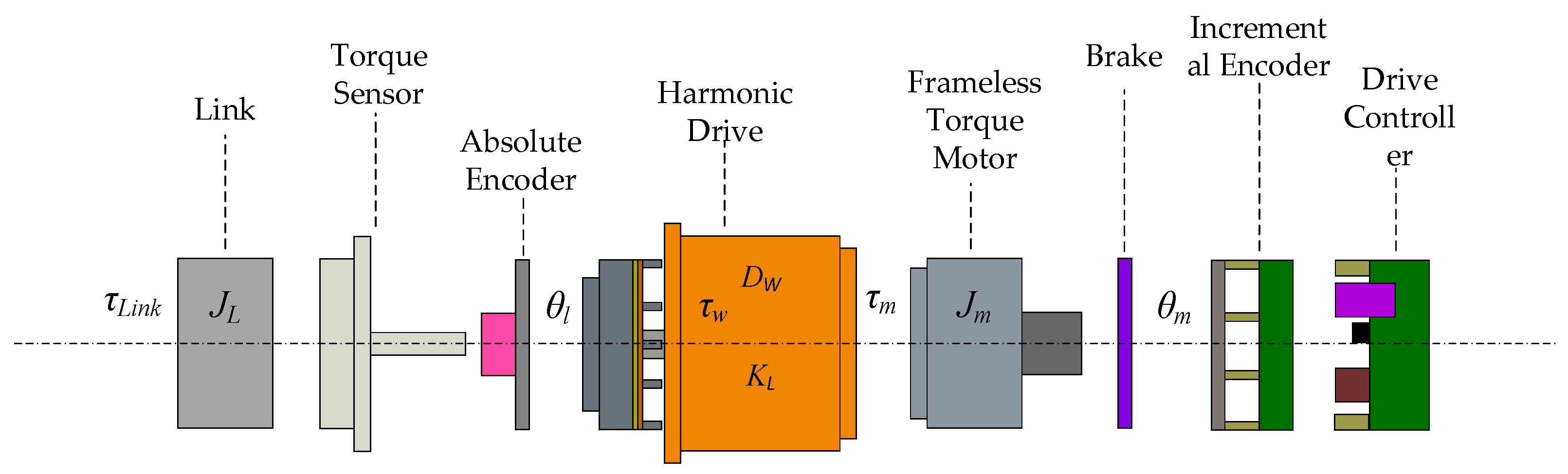
In the absence of considering factors such as joint vibration and flexibility, the servo motor and the load end are regarded as rigid bodies to improve the basic identification accuracy as much as possible. However, in actual situations, the motor and the load end are not directly coupled, but rather form an elastic system, and the joint bearings and outer frame are not completely rigid. Under the action of motor drive torque, mechanical deformation occurs. Mechanical resonance has a certain effect on the dynamic performance of the system, mainly due to harmonic reducers, and the joint physical model is shown in Figure 3. Therefore, for joint systems that have requirements for accuracy and speed, elastic deformation cannot be ignored. This principle can be used to estimate the torque component during mechanical resonance in reverse. Another significant torque component can be estimated directly through current, while compensating for frictional forces, which will result in a better effect.

The servo drive section is located on the right; the link end is located on the left, with the harmonic reducer transmission device being in the center. The servo motor drives the entire executing mechanism, and its position is measured with an incremental encoder. The position of the link end is measured with an absolute value encoder. The position and velocity of the motor-side encoder are converted to the link side through the reduction ratio. Thus, the theoretical and actual errors can be calculated to determine the deformation. The joint module is driven by a coupled drive, which results in the servo system becoming a highly coupled and multi-inertia system. For ease of study, the system can be simplified into a flexible connected servo system with two inertias. ${\mathit{\tau }}_w$ represents the harmonic resonance torque component caused by the harmonic reducer, and ${\mathit{\tau }}_m$ is generally directly obtained from the motor without taking this into account. J_m and J_l refer to the rotational inertia of the motor and the link, respectively. K_w is the transmission coupling stiffness coefficient while D_w is the transmission shaft damping coefficient. ${\mathit{\theta }}_m$ and ${\mathit{\theta }}_l$ are, respectively, the theoretical angle calculated to the link side and the actual angle of the link side. Due to the challenging friction modeling and accurate modeling of the harmonic link and torque transmission error, errors occur. Also, the acceleration is measured inaccurately prone to fluctuations, and filtering causes errors. Therefore, the torque generated by J_m${\ddot{\mathit{\theta }}}_m$ is not taken into account, and the following text will incorporate it into the error. Based on the traditional dynamic model, this paper calculates the difference between the model torque and the actual torque, and analyzes it using an error model and data model analysis. To utilize dynamic compensation, the torque ${\mathit{\tau }}_w$ is no longer used, and the torque ${\mathit{\tau }}_u$ is defined.

$${\mathit{\tau }}_m={\mathit{\tau }}_f+{\mathit{\tau }}_u+{\mathit{\tau }}_{link}$$

(26)

An effective and relatively fast method, which is designed as a unified three-loop iterative scheme [21], is proposed to acquire an accurate dynamic model, but does not compensate for unmodeled torque or harmonics. This paper proposes an improved version of the three-loop method. The first loop identifies the friction force, the second loop identifies the ${\mathit{\tau }}_{link}$ of the link dynamic, and the third loop compensates for uncertain components using flexible error to improve accuracy. If the torque component ${\mathit{\tau }}_u$ cannot be accurately modeled, direct application of the learning method will lead to over-reliance on data. Furthermore, the linear modeling method suggested in [6] shows poor accuracy in some states, and estimation is impossible without flexible deformation. This paper proposes a method based on double-encoder information for identifying the residual torque. This method is designed to enable nonlinear approximation and smoothing of the residual torque, effectively solving the problems mentioned above. For the nonlinear f(·) part, it is inspired by the methods similar to DMP (Dynamic Movement Primitives) and RBF (radial basis function) in [30] to fit the nonlinear part. The radial basis function is

$${\psi }_j(u)=\exp \left(-\frac{1}{2{\sigma }_j^2}{(u-c_j)}^2\right),j=1,2,\dots ,N$$

(27)

$\sigma$ represents the width of the radial basis function, c represents its center position, and the number of basis functions is N. Since offline identification is used to obtain weight coefficients, it is hoped that the fitting parameters have high compatibility, and the error limit of ${\theta }_m$−${\theta }_l$ is defined as $∆{\theta }_{max}$,$∆{\theta }_{min}$; then, the calculation method of ${\sigma }_i$ and c_i is

$$\{\begin{array}{l}{c}_j=\Delta {\theta }_{\min }+(j-1)\left(\frac{\Delta {\theta }_{\max }-\Delta {\theta }_{\min }}{N-1}\right)\\ {\sigma }_j=\frac{1}{{(0.5(c_{j+1}-c_j))}^2}\end{array}$$

(28)

In the same way, operating on ${\dot{\theta }}_m$−${\dot{\theta }}_l$, ${\sigma }_j$ only needs to expand one data value at the end to satisfy data synchronization, so that the values of $c_j$ and ${\sigma }_j$ can be determined. Ensure that the Gaussian function covers the entire flexible error space of the industrial robot, and has an effective mapping for the input u of the RBF network. If the traditional RBF network is used to fit the data, it is necessary to update the center position, width, and weight of the radial basis function. However, increasing the amount of program also modifies the coverage interval of the radial basis function, which is unfavorable for dynamic identification, so [${\theta }_m$−${\theta }_l$, ${\dot{\theta }}_m$−${\dot{\theta }}_l$] needs to be identified uniformly, so as to reflect the uncertain torque components under different joint states. Assume that the number of radial basis functions is N, and the data have M groups:

$$f(u)=\frac{{\displaystyle \sum _{i=1}^N{w}_{rj}}{\psi }_j(u)}{{\displaystyle \sum _{j=1}^N{\psi }_j}(u)}$$

(29)

It is necessary to identify all the data at one time, and the expected fitting data are f_target = [f_target(1), f_target(2),…f_target(M)]; then, the weight identification is

$$\left[\begin{array}{llll}{\psi }_1(1)\hfill & {\psi }_1(2)\hfill & \cdots \hfill & {\psi }_N(M)\hfill \\ {\psi }_2(1)\hfill & {\psi }_2(2)\hfill & \cdots \hfill & {\psi }_N(M)\hfill \\ ⋮\hfill & ⋮\hfill & \cdots \hfill & ⋮\hfill \\ {\psi }_N(1)\hfill & {\psi }_N(2)\hfill & \cdots \hfill & {\psi }_N(M)\hfill \end{array}\right]\cdot \left[\begin{array}{l}{f}_{target}(1)\\ f_{target}(2)\\ ⋮\\ f_{target}(m)\end{array}\right]=\left[\begin{array}{l}{w}_{r1}{\displaystyle \sum _{j=1}^M{\psi }_1(i)}\\ w_{r2}{\displaystyle \sum _{j=1}^M{\psi }_2(i)}\\ ⋮\\ w_{rN}{\displaystyle \sum _{j=1}^M{\psi }_N(i)}\end{array}\right]$$

(30)

Directly calculate the network weight W_r = [w_r1, w_r2, …, w_rN]; the actual process needs to [${\theta }_m$−${\theta }_l$, ${\dot{\theta }}_m$−${\dot{\theta }}_l$] as the input data, and torque ${\mathit{\tau }}_u$ as the expected training.

Due to the multi-degree-of-freedom serial structure of robotic manipulators, employing a single neural network alone cannot adequately capture the coupling between joints. Therefore, a GMM (Gaussian Mixture Model) is employed to model each joint of the multi-degree-of-freedom robotic manipulator. Subsequently, GMR (Gaussian Mixture Regression) is applied to fit the data for each joint individually. This approach is essential for accurately characterizing the intricate interdependencies among the joints in multi-degree-of-freedom robotic arms.

GMM (Gaussian Mixture Model) assumes that data are composed of multiple Gaussian distributions, each referred to as a component, and a data point may originate from any one of these components. Model parameters include the mean, covariance matrix, and weight for each component. These parameters are estimated using the EM (Expectation–Maximization) algorithm, where the E-step calculates the probability of each data point belonging to each component, and the M-step updates the model parameters. The EM algorithm is an iterative optimization algorithm used to estimate parameters in models with latent variables. It comprises two steps: the Expectation step and Maximization step. The E-step computes the expectation of latent variables for observed data given the current parameters. The M-step maximizes the expectation calculated in the E-step, updating model parameters. GMR (Gaussian Mixture Regression) is a regression model that uses GMM to model the conditional probability distribution, capturing the relationship between input and output. GMM parameters are estimated using the EM algorithm. Given input data, conditional probability distribution is computed using GMM, followed by the calculation of the expected value and variance of the output. This is commonly used for modeling complex nonlinear relationships. In summary, the fundamental idea of the GMM EM GMR algorithm is to model data using GMM, iteratively optimize model parameters with the EM algorithm, and then apply these parameters in GMR to establish the relationship between input and output for predictive purposes.

The modeling and regression process for the i-th joint is as follows: In the first step, data from joint i are ${\xi }_i=\left\{u_i,f\left(u_i\right)\right\}$, with ${\xi }_i\in {\mathbb{R}}^{3\times m}$, $u_i\in {\mathbb{R}}^{2\times m}$ comprising an input vector consisting of joint position and velocity, where $f\left(u_i\right)\in {\mathbb{R}}^m$ represents the output vector composed of joint torque residuals, and m represents the number of sampled points in the dataset. The second step involves modeling the dataset $\xi$ using a GMM consisting of K Gaussian components. The joint probability density of the GMM is defined as follows:

$$p({\xi }_i)={\displaystyle \sum _{k=1}^K{\pi }_k}N({\xi }_i;{\mu }_k,{\sum }_k)$$

(31)

In the equation, ${\pi }_1,\dots ,{\pi }_K$ represents the mixture coefficient for the k-th Gaussian component, subject to the constraints${\pi }_k>0$ and ${\sum }_{k=1}^K{\pi }_k=1$. ${\mu }_1,\dots {,\mu }_K$ denotes the mean of the k-th Gaussian component, and ${\mathsf{\Sigma }}_1,\dots ,{\mathsf{\Sigma }}_K$ is the covariance matrix associated with it. $N({\mu }_1,{\mathsf{\Sigma }}_k)$ represents the Gaussian component defined by mean ${\mu }_k$ and covariance ${\mathsf{\Sigma }}_k$. Specifically, the k-th Gaussian component is defined as follows:

$$p({\xi }_i|{\mu }_k,{\sum }_k)=\frac{1}{2\pi \sqrt{\left|{\sum }_k\right|}}{e}^{-\frac{1}{2}({({\xi }_i-{\mu }_k)}^T{\sum }_k^{-1}({\xi }_i-{\mu }_k))}$$

(32)

The third step involves utilizing the EM algorithm to compute the parameters ${\pi }_k$, ${\mu }_k$, and ${\mathsf{\Sigma }}_k$ for each Gaussian component.

In the fourth step, after obtaining the GMM parameters, GMR is employed to fit the expected function $f\left(\text{∙}\right)$. For each Gaussian component, given the input data $u_i$, the conditional probability $f\left(u_i\right)$ satisfies a Gaussian distribution.

$$p(f(u_i)|u_i,k)=N(f(u_i);\widehat{f}(u_i),{\widehat{\sum }}_{f(u_i),k})$$

(33)

$${\widehat{f}}_k(u_i)={\mu }_{f(u_i),k}+{\sum }_{f(u_i)u_i,k}{({\sum }_{u_i,k})}^{-1}(u_i-{\mu }_{u_i,k})$$

(34)

$${\widehat{\sum }}_{f(u_i),k}={\sum }_{f(u_i),k}-{\sum }_{f(u_i)u_i,k}{({\sum }_{u_i,k})}^{-1}{\sum }_{u_{i}f(u_i),k}$$

(35)

$$p(f(u_i)|u_i)={\displaystyle \sum _{k=1}^K{h}_k(u_i)}N(f(u_i);{\widehat{f}}_k(u_i),{\widehat{\sum }}_{f(u_i),k})$$

(36)

$$h_k(u_i)=\frac{p(k)p(u_i|k)}{{\sum }_{i=1}^{K}p(i)p(u_i|i)}=\frac{{\pi }_{k}N(u_i;{\mu }_{u_i,k},{\sum }_{u_i,k})}{{\sum }_{i=1}^K{\pi }_{i}N(u_i;{\mu }_{u_i,k},{\sum }_{u_i,k})}$$

(37)

The estimation of the conditional expectation $f\left(u_i\right)$ given $u_i$ under the Gaussian distribution is defined using the linearity property. The parameters of the Gaussian distribution are defined as

$$\widehat{f}(u_i)={\displaystyle \sum _{k=1}^K{h}_k(u_i)}{\widehat{f}}_k(u_i)$$

(38)

$${\widehat{\sum }}_{f(u)}={\displaystyle \sum _{k=1}^K{h}_k^2(u)}{\widehat{\sum }}_{f(u),k}$$

(39)

The above equation represents the torque residual $\widehat{f}\left(u_i\right)$ fitted under joint position and joint velocity $u_i$ for the i-th joint.

6. Simulation and Experiment

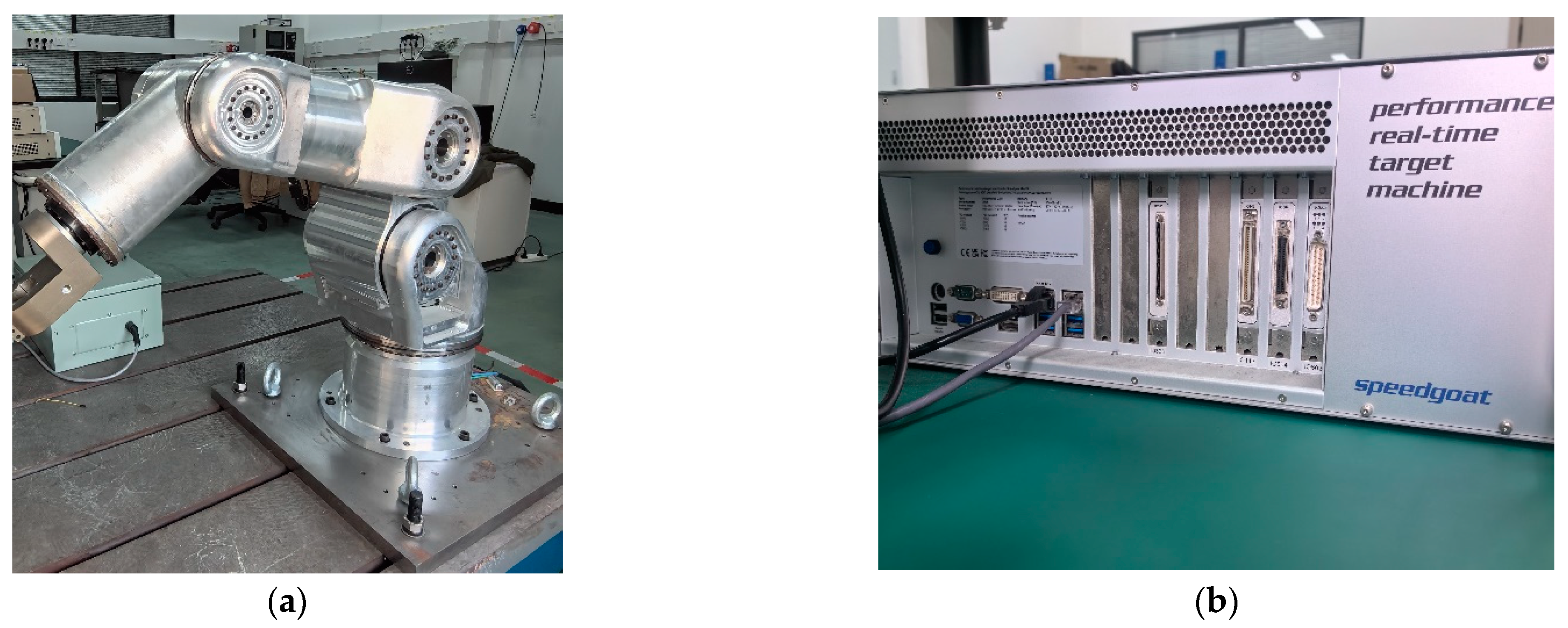
To illustrate the proposed method, several experiments were undertaken on the 6-DoF industrial robot. The experiment system is shown in Figure 4, and the controller’s hardware platform is equipped with a SpeedGoat RCP (The SpeedGoat, Bern, Switzerland) real-time simulation platform [31] that has a computation cycle of 1 ms. The control system is developed with the MDH model, utilizing the real-time function of MATLAB Simulink (The MathWorks, Natick, USA). The computer in use is equipped with a CPU: I7-11800H-2.30 GHz, 64 G-3200 MHZ memory, and the MATLAB version is 2022b.

In this paper, the fifth-order Fourier series is used to design the exciting trajectory. The exciting frequency of the trajectory is $f_{\mathrm{s}}=0.02\mathrm{Hz}$, and the cycle is 20 s. The displacement, velocity, and acceleration of each joint are calculated using the Fourier series, to obtain 200 discrete points every 0.1 s. The constraint limits of the joint displacements, velocities, and accelerations of the industrial robots used in the experiment are shown in

Table 1. The parameters of exciting trajectory limits.

Limits		Joint 1	Joint 2	Joint 3	Joint 4	Joint 5	Joint 6
Joint limit ${\theta }_{I,max}$ (deg)	Max	120	90	60	120	120	120
	Min	−120	−90	−60	−120	−120	−120
Joint velocity limit ${\dot{\theta }}_{I,max}$ (deg/s)	Max	100	60	60	80	80	80
	Min	−100	−60	−60	−80	−80	−80
Joint acceleration limit ${\ddot{\theta }}_{I,max}$ (deg/s2)	Max	120	120	120	120	120	120

.

Comparing the condition number of the regression matrix obtained with the optimization index method based on the block regression matrix condition number and the least squares method used in this paper, the results are shown in

Table 2. Comparison table of condition number optimization results of different methods.

Optimization Method	Condition Number
WLS	189.4012
Ours	162.2440

below:

It can be seen from Table 2 that the condition number of the regression matrix obtained with the method used in this paper is the smallest. At the same time, the method used in this paper optimizes the sub-matrix of the regression matrix and adjusts the internal structure of the regression matrix, so it can better stimulate the characteristics of the dynamic parameters. Because there are six joints, the number of variable coefficients for the total trajectory optimization solution is 66. According to the constraint parameters provided in Table 1, the coefficients of the exciting trajectory are calculated through the pattern search optimization function provided using Matlab, as shown in

Table 3. Coefficient results of exciting trajectories.

Optimization Parameters	Joint 1	Joint 2	Joint 3	Joint 4	Joint 5	Joint 6
al,i	0.0046 −0.0074 0.4845 −0.5103 0.0286	−0.0406 0.0597 0.2492 0.0678 −0.3361	−0.1772 0.0661 0.1019 0.0189 −0.0097	−0.1704 0.1161 −0.1703 0.1426 0.0820	−0.0210 −0.1317 0.3614 −0.1994 −0.0094	0.0673 0.2685 0.1682 −0.4241 −0.0763
bl,i	−0.0053 −0.0182 0.6963 −0.3354 −0.1411	−0.0234 −0.2122 0.1619 −0.1082 0.0789	−0.0001 −0.0583 0.0450 0.1273 −0.1056	0.0088 −0.3357 0.1996 0.1731 −0.1257	0.1460 −0.3491 0.3639 −0.1008 −0.0273	0.1335 0.0677 0.0942 −0.2907 0.1227
${\theta }_{i0}\left(\mathrm{rad}\right)$	0.3361	−0.2762	−0.0112	−0.2369	0.1976	0.4777

. The total system runtime is determined by the maximum integer time. Loop1 corresponds to the friction identification module, taking 1 s to complete. Loop2 represents the dynamics identification module, where the trajectory optimization and execution take 30 s, and the dynamic parameter identification process requires 5 s. Loop3 corresponds to the dynamics compensation module based on dual-encoder deformation. The GMM algorithm within this module has a relatively longer runtime, contributing to the total module time of 2 s.

The actual running period of the industrial robot is set to 20 s, and the displacement, velocity, and acceleration of each joint exciting trajectory are shown in Figure 5.

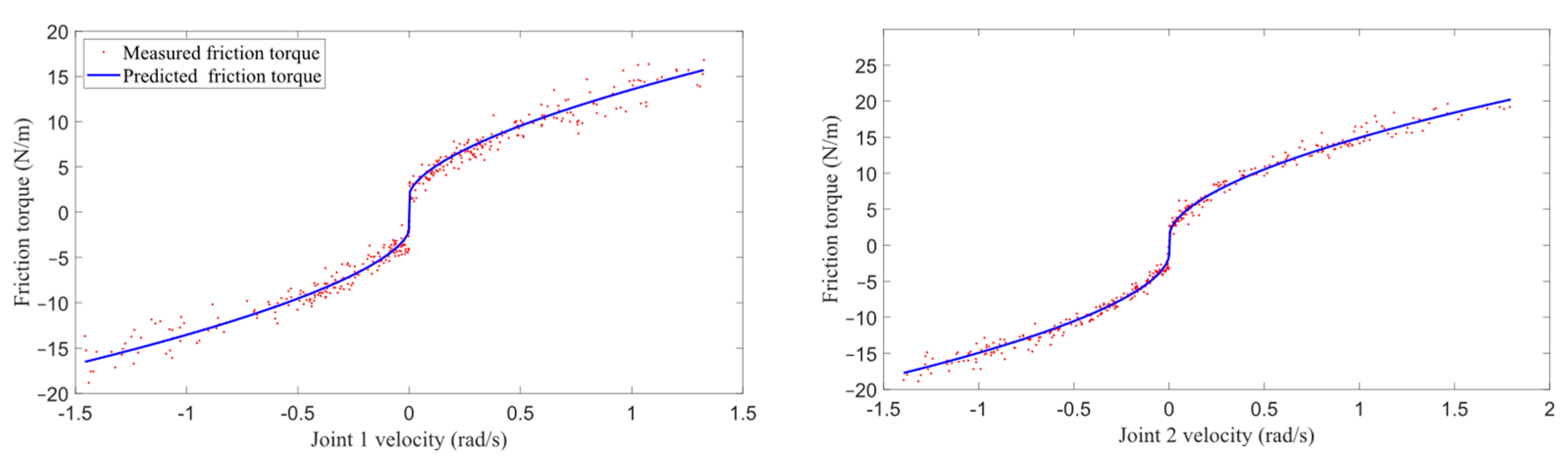
The rotation axis of Joint 1 is orthogonal to that of Joint 2, with minimal gravitational impact on Joint 1 and maximal gravitational impact on Joint 2. Consequently, selecting the friction between Joint 1 and Joint 2 as the test parameter for the algorithm is a compelling choice. Figure 6 illustrates the ultimate results of Joint 1 and Joint 2 friction estimation along with the fitting parameters. The nonlinear parameters prove to be highly effective in capturing the friction characteristics under conditions close to zero. Tailoring to specific requirements, more sophisticated friction models can be seamlessly integrated into the proposed framework.

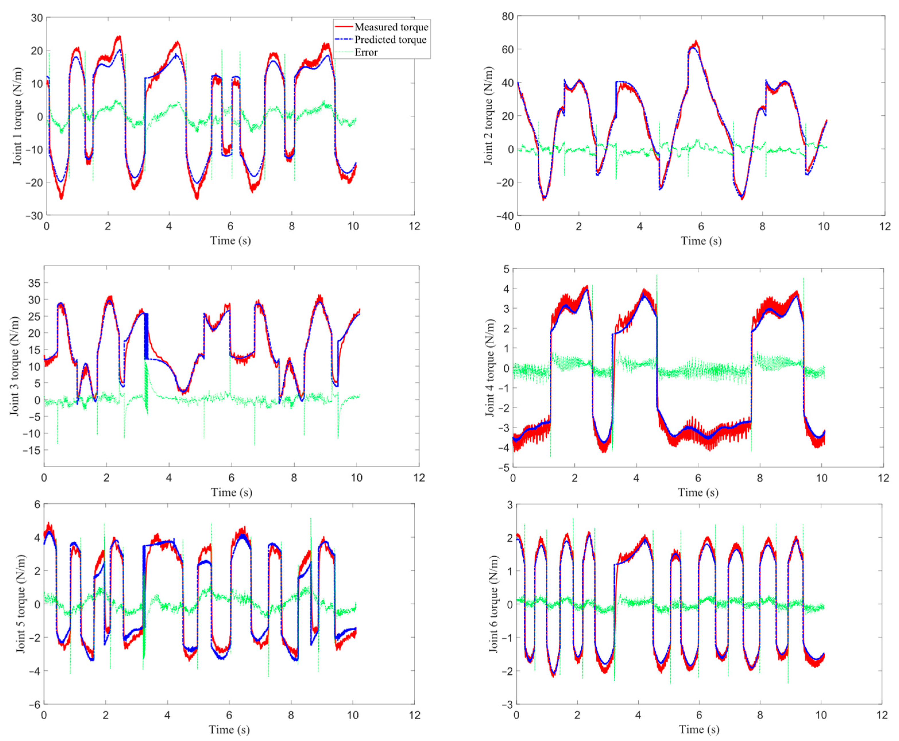
Directly use the traditional WLS method to identify the dynamic model and friction of the link. Observing the results in Figure 7, it can be found that the effect is not ideal, and even when the joint moves smoothly in one direction, a large error occurs. As long as the joints are in motion, there will be joint deformations. At this time, only the encoder on the link side is used for dynamic identification, and there will be errors. When the joints return to the zero position, the industrial robot is in a vertical state at this time, and there is almost no motion deformation in each joint, so the residual torque is almost zero. Finally, we compensate for the residual torque based on the double-encoder information, and Figure 8 shows the results of the identification method proposed in this paper.

Given that the identification framework in this paper is also based on an iterative strategy, our proposed method exhibits a notable improvement in torque estimation, particularly in turning and local positions compared to the WLS method. The collection of torque and joint state data introduces high-frequency noise, originating from joint and mechanical vibrations, as well as friction forces that cannot be precisely estimated. To address this, we introduce low-pass filtering for effective noise reduction, ensuring a more accurate representation of torque information without compromising the signal.

In Figure 7 and Figure 8, it can be seen that the dynamic model identified with the method used in this paper is more accurate, and the measured torque basically agrees with the predicted torque current. The calculated RMSE (root mean square error) between the predicted torque and the actual measured torque of each joint is shown in

Table 4. Result of RMSE.

Identification Method	Joint 1	Joint 2	Joint 3	Joint 4	Joint 5	Joint 6
WLS	2.3376	2.1278	1.5395	0.3361	0.7101	0.2578
Ours	1.9594	1.7345	1.1609	0.3027	0.5852	0.2096

. The results show that the three-loop dynamics identification scheme based on double-encoder information compensation proposed in this paper has a significant improvement compared with the WLS, and the RMSE of the residual torque is reduced by more than 20%, which proves the superiority of the method in this paper compared with the traditional method.

7. Conclusions

The method proposed in this paper firstly identifies the friction force through two directional moments, and then conducts a theoretical identification on the dynamics of the link, in which the block matrix condition number is used as the optimization index for the exciting trajectory. Finally, the deformation moments that cannot be accurately modeled are estimated using double-encoder information, which can reflect the influence of unmodeled parts such as harmonic reducers. The dynamic parameter identification of an industrial robot has been enhanced in two aspects. Firstly, a nonlinear friction force model, distinguishing between high and low speeds, is employed to better fit the dynamic friction effects of the robotic arm. Secondly, the GMM algorithm is introduced into dynamic parameter identification to compensate for the uncertain torque residue arising from nonlinear fitting. However, through an intuitive analysis of the residual torque, it can be found that the accuracy of the torque estimation will decrease in the place where the speed switches direction, and the error will be large. This is also due to the difficulty in estimating the friction force when the movement switches directions. This approach reduces the root mean square of identification residuals by 20%, signifying a significant improvement in the precision of model parameter identification.