A Sliding Mode Control-Based Guidance Law for a Two-Dimensional Orbit Transfer with Bounded Disturbances

Abstract

The aim of this paper is to analyze the performance of a state-feedback guidance law, which is obtained through a classical sliding mode control approach, in a two-dimensional circle-to-circle orbit transfer of a spacecraft equipped with a continuous-thrust propulsion system. The paper shows that such an inherently robust control technique can be effectively used to obtain possible transfer trajectories even when the spacecraft equations of motion are affected by perturbations. The problem of the guidance law design is first addressed in the simplified case of an unperturbed system, where it is shown how the state-feedback control may be effectively used to obtain simple mathematical relationships and graphs that allow the designer to determine possible transfer trajectories that depend on a few control parameters. It is also shown that a suitable combination of the controller parameters may be exploited to obtain trade-off solutions between the flight time and the transfer velocity change. The simplified control strategy is then used to investigate a typical heliocentric orbit raising/lowering in the presence of bounded disturbances and measurement errors.

1. Introduction

In a preliminary phase of mission design, the use of a state-feedback control law represents a viable option to obtain possible transfer trajectories that may be used as an initial starting point for succeeding (and more refined) analyses. In this context, an interesting approach is based on the use of a rather classical sliding mode control, which is a variable structure (control) method that alters the dynamical behaviour of a nonlinear system through the application of a suitable control signal [1]. In particular, sliding mode control is a basic robust technique, which allows the system trajectory to converge towards the desired target even in the presence of significant perturbations and measurement errors [2,3]. An interesting discussion about the potentialities of a sliding mode control law can be found in the review paper by Hung et al. [4] and in the work by Utkin [5].

The literature about the control of satellites by means of sliding mode techniques is rich, although essentially concentrated on attitude control and terminal guidance maneuvers [6]. In this scenario, Wu et al. [7] investigated the attitude synchronization and tracking problem including model uncertainties, external disturbances, actuator failures, and control torque saturation. By proposing two decentralized sliding mode control laws, that work [7] proved that the control laws guarantee each spacecraft to approach the desired time-varying attitude and angular velocity while maintaining attitude synchronization among the other elements in a typical formation structure. Another example is offered by the work by Massey and Shtessel [8], who adopted a traditional, continuous, high-order sliding mode strategy to control a satellite formation in a robust manner (i.e., compensating for model uncertainties and external disturbances). An adaptive sliding mode tension control method was successfully proposed by Ma et al. [9] for the deployment of tethered satellites, when input tension limitations are taken into account. On the other hand, a terminal sliding mode control law was designed by Liu and Huo [10] for spacecraft rendezvous and docking while considering both model uncertainties and external disturbances, proving that the closed-loop tracking error converges to zero in a finite time. The same problem was also successfully addressed by Dong et al. [11], who constructed a nonsingular terminal sliding surface by introducing a continuous sinusoidal function to solve the inherent singularity problem. More recently, Capello et al. [12] designed two controllers, that is, a first-order sliding mode control for position tracking and a supertwisting second-order sliding mode control for attitude stability, in which the mutual influence was taken into account by the introduction of additional disturbances. Kasaeian et al. [13] presented a robust guidance algorithm to perform a rendezvous between a chaser and a target spacecraft orbiting around the Earth, revealing that sliding mode control guarantees the tracking of the required states and minimum final errors even in the presence of uncertainties and disturbances. Li et al. [14] developed a novel sliding mode control strategy to address the relative position tracking and attitude synchronization problem of spacecraft rendezvous with the requirement of collision avoidance, proving the convergence of relative position and attitude errors even in the presence of external disturbances. Finally, Bassetto et al. [15] discussed how solar sail attitude maneuvers may be designed in a collinear, artificial, equilibrium point by implementing a sliding mode control strategy that uses electrochromic devices as actuators [16,17,18]. Anyway, there are many other potential feedback control techniques [19,20,21], to which the interest reader is invited to refer.

In the context of spacecraft trajectory design, a robust state-feedback control law can be used to obtain a possible transfer trajectory that is useful as an initial guess during the subsequent refinement phase [22]. In that case, potential transfer trajectories can be obtained by taking into account the orbit perturbations and the model uncertainties with a reduced computational cost [23]. The aim of this paper is to investigate the potentialities of a sliding mode control strategy in detecting possible trajectories in a typical circle-to-circle orbit transfer scenario, in which the spacecraft propulsion system provides a continuously adjustable and freely steerable propulsive acceleration vector. Among actuators capable of generating variable propulsive acceleration, there are variable thrust ion engines (such as NASA’s Evolutionary Xenon Thruster (NEXT)), in which continuous thrust variation can be replaced by a succession of discrete thrust levels that, on average, provide the required propulsive acceleration. For example, NEXT has a total of 40 operating points, with available thrust ranging from $25.5\mathrm{mN}$ and $236\mathrm{mN}$ [24]. The proposed approach uses a standard implementation of the sliding mode procedure [1] to obtain a set of preliminary results. In this way, the discussed procedure allows the designer to make a trade-off between the flight time and the required velocity change by selecting the design parameters of the controller. In particular, the simplified control strategy involves three independent parameters of the spacecraft dynamics (on which the resulting propulsive acceleration profile and the characteristics of the transfer trajectory depend), which represent tuning quantities to be selected by the designer. The main limitation of the proposed approach lies in the use of an ideal propulsion system to control the nonlinear dynamics of the spacecraft center of mass. In fact, the time-variation of the thrust vector magnitude, which is an output of the design procedure, can be used a posteriori to check whether the obtained transfer trajectory is compatible with the physical constraints of the thruster, such as the maximum thrust level.

Starting from the simplified scenario, in which the spacecraft orbital dynamics is unaffected by external disturbances or model uncertainties, we firstly discuss how the controller may be tuned by considering the flight time and total velocity change. The procedure is then used to investigate an orbit raising/lowering in the presence of bounded disturbances and measurement errors. The paper is organized as follows. Section 2 presents the mathematical model, i.e., the nonlinear differential equations describing the coplanar orbital motion of a spacecraft around an assigned primary body. Section 3 introduces the sliding mode control technique in its general form, where bounded disturbances are included in the model. Section 4 addresses the design of the sliding mode control law in the simplified case of an unperturbed system. In particular, Section 4 illustrates the time-variation of tracking errors (which can be analytically determined when no disturbance is considered in the mathematical model) and the definition of the control law parameters. The numerical simulations are described in Section 5, while the concluding remarks are drawn in Section 6.

2. Problem Description and Mathematical Model

Consider a spacecraft S that covers a circular parking orbit of radius $r_0$ around a primary body with center of mass P and gravitational parameter $\mu$. The mission purpose is to transfer the spacecraft to a circular and coplanar target orbit of assigned radius $r_f\ne r_0$ by means of a continuously adjustable (and freely steerable) propulsion system, which gives both a radial ($a_r$) and a transverse ($a_t$) component of propulsive acceleration. In this context, the spacecraft two-dimensional dynamics may be described by the classical polar equations of motion [25]:

$$\begin{array}{cc}\hfill \dot{r}& =v_r\hfill \end{array}$$

(1)

$$\begin{array}{cc}\hfill \dot{\theta }& ={\displaystyle \frac{v_t}{r}}\hfill \end{array}$$

(2)

$$\begin{array}{cc}\hfill {\dot{v}}_r& =-{\displaystyle \frac{\mu }{r^2}}+{\displaystyle \frac{v_t^2}{r}}+d_r+a_r\hfill \end{array}$$

(3)

$$\begin{array}{cc}\hfill {\dot{v}}_t& =-{\displaystyle \frac{v_r{v}_t}{r}}+d_t+a_t\hfill \end{array}$$

(4)

where r is the P-S distance and $\theta$ is the spacecraft polar angle measured counterclockwise from the P-S line at the initial time $t_0\triangleq 0$, while $v_r$ (or $v_t$) is the radial (or transverse) component of the spacecraft velocity vector; see Figure 1. In Equations (3) and (4), the terms $\{d_r,d_t\}$ represent possible unknown bounded disturbance accelerations acting along the radial and transverse directions, with

$$|d_r|\le D_r,|d_t|\le D_t$$

(5)

where $D_r\ge 0$ and $D_t\ge 0$ are two constant parameters.

Bearing in mind that the parking orbit is circular, Equations (1)–(4) are completed by the initial conditions

$$r\left(t_0\right)=r_0,\theta \left(t_0\right)=0,v_r\left(t_0\right)=0,v_t\left(t_0\right)=\sqrt{\mu /r_0}$$

(6)

while the time-variation of the propulsive acceleration components $\{a_r,a_t\}$ are to be found so as to bring the spacecraft states to the desired final values

$$r\left(t_f\right)=r_f,v_r\left(t_f\right)=0,v_t\left(t_f\right)=\sqrt{\mu /r_f}$$

(7)

within a time interval $t_f$. Note that the final polar angle $\theta \left(t_f\right)$, that is, the angle swept out by the spacecraft during the transfer, is left free.

The spacecraft dynamics is more conveniently rewritten by introducing the dimensionless tracking errors in radial distance ($x_1$), radial velocity component ($x_2$), and transverse velocity component ($x_3$), defined as

$$\begin{array}{cc}\hfill x_1& \triangleq {\displaystyle \frac{r-r_f}{r_0}}\equiv {\displaystyle \frac{r}{r_0}}-\rho \hfill \end{array}$$

(8)

$$\begin{array}{cc}\hfill x_2& \triangleq {\displaystyle \frac{v_r}{\sqrt{\mu /r_0}}}\hfill \end{array}$$

(9)

$$\begin{array}{cc}\hfill x_3& \triangleq {\displaystyle \frac{v_t-\sqrt{\mu /r_f}}{\sqrt{\mu /r_0}}}\equiv {\displaystyle \frac{v_t}{\sqrt{\mu /r_0}}}-{\displaystyle \frac{1}{\sqrt{\rho }}}\hfill \end{array}$$

(10)

where $\rho \triangleq r_f/r_0\ne 1$ is the dimensionless radius of the target circular orbit. In particular, $\rho \in (0,1)$ in case of an orbit lowering, whereas $\rho >1$ in case of an orbit raising. Substituting Equations (8)–(10) into Equations (1), (3), and (4) yields

$$\begin{array}{cc}\hfill x_1^{\prime }& =x_2\hfill \end{array}$$

(11)

$$\begin{array}{cc}\hfill x_2^{\prime }& =-{\displaystyle \frac{1}{{\left(x_1+\rho \right)}^2}}+{\displaystyle \frac{{\left(x_3+1/\sqrt{\rho }\right)}^2}{x_1+\rho }}+z_r+u_r\hfill \end{array}$$

(12)

$$\begin{array}{cc}\hfill x_3^{\prime }& =-{\displaystyle \frac{x_2\left(x_3+1/\sqrt{\rho }\right)}{x_1+\rho }}+z_t+u_t\hfill \end{array}$$

(13)

where the prime symbol denotes a derivative taken with respect to the dimensionless time $\tau$, defined as

$$\tau \triangleq {\displaystyle \frac{t}{\sqrt{r_0^3/\mu }}}$$

(14)

with $\tau \left(t_0\right)={\tau }_0\triangleq 0$, while

$$u_r\triangleq {\displaystyle \frac{a_r}{\mu /r_0^2}},u_t\triangleq {\displaystyle \frac{a_t}{\mu /r_0^2}}$$

(15)

are the two dimensionless control variables, defined as the ratio of the propulsive acceleration components $\{a_r,a_t\}$ to the primary body gravitational acceleration at $r=r_0$. Finally, the two terms $\{z_r,z_t\}$ in Equations (12) and (13) are the dimensionless forms of the disturbance acceleration components, defined as

$$z_r\triangleq {\displaystyle \frac{d_r}{\mu /r_0^2}},z_t\triangleq {\displaystyle \frac{d_t}{\mu /r_0^2}}$$

(16)

which, by assumption, satisfy the inequalities

$$|z_r|\le Z_r\triangleq {\displaystyle \frac{D_r}{\mu /r_0^2}},|z_t|\le Z_t\triangleq {\displaystyle \frac{D_t}{\mu /r_0^2}}$$

(17)

Equations (11)–(13) are integrated with the three initial conditions

$$x_1\left({\tau }_0\right)=x_{1_0}\triangleq 1-\rho ,x_2\left({\tau }_0\right)=x_{2_0}\triangleq 0,x_3\left({\tau }_0\right)=x_{3_0}\triangleq 1-1/\sqrt{\rho }$$

(18)

from which it follows that $x_{1_0}<0$ and $x_{3_0}>0$ when $\rho >1$, while $x_{1_0}>0$ and $x_{3_0}<0$ when $\rho \in (0,1)$. Finally, the target states (i.e., the conditions on the target circular orbit) are expressed in a dimensionless form as

$$x_1\left({\tau }_f\right)=x_{1_f}\triangleq 0,x_2\left({\tau }_f\right)=x_{2_f}\triangleq 0,x_3\left({\tau }_f\right)=x_{3_f}\triangleq 0$$

(19)

where

$${\tau }_f\triangleq {\displaystyle \frac{t_f}{\sqrt{r_0^3/\mu }}}$$

(20)

is the dimensionless flight time. Note that the $\tau$-variation of $\theta$ can be obtained by numerically integrating the differential equation

$${\theta }^{\prime }={\displaystyle \frac{x_3+1/\sqrt{\rho }}{x_1+\rho }}$$

(21)

which is not included in the dynamical system because the final polar angle is left free. However, solving Equation (21) is necessary to obtain the polar trajectory of the spacecraft.

3. State-Feedback Control Design

In this section, a classical sliding mode control law is used to determine the circle-to-circle orbit transfer trajectory. The spacecraft states are brought and maintained on two sliding surfaces, where the system exhibits the desired dynamics of reduced order or one of the states is at its final equilibrium point. More specifically, the first sliding surface is described by the equation

$$s\triangleq x_2+\lambda x_1=0$$

(22)

where $\lambda >0$ is a dimensionless design parameter, so that the states $\{x_1,x_2\}$ exhibit a first-order dynamics when the system is on that sliding surface. In fact, bearing in mind Equation (11), the condition $s=0$ implies

$$x_2=x_1^{\prime }=-\lambda x_1$$

(23)

from which the $\tau$-variations of the tracking errors $\{x_1,x_2\}$ turn out to be proportional to $e^{-\lambda \tau }$, viz.

$$x_1\left(\tau \right)\propto e^{-\lambda \tau },x_2\left(\tau \right)\propto \lambda e^{-\lambda \tau }$$

(24)

In other terms, when the system is brought to the sliding surface $s=0$, both $x_1$ and $x_2$ converge exponentially to zero with a convergence rate equal to $\lambda$.

Now, in order to bring the system on the sliding surface $s=0$, it is required that $s^{\prime }<0$ when $s>0$, and $s^{\prime }>0$ when $s<0$. To this end, differentiating s with respect to $\tau$ yields

$$s^{\prime }=x_2^{\prime }+\lambda x_1^{\prime }\equiv -{\displaystyle \frac{1}{{\left(x_1+\rho \right)}^2}}+{\displaystyle \frac{{\left(x_3+1/\sqrt{\rho }\right)}^2}{x_1+\rho }}+z_r+u_r+\lambda x_2$$

(25)

from which selecting $u_r$ according to the law

$$u_r={\displaystyle \frac{1}{{\left(x_1+\rho \right)}^2}}-{\displaystyle \frac{{\left(x_3+1/\sqrt{\rho }\right)}^2}{x_1+\rho }}-\lambda x_2-\delta \mathrm{sign}\left(s\right)$$

(26)

where $\mathrm{sign}\left(\square \right)$ is the signum function and $\delta$ is given by

$$\delta \triangleq Z_r+K>0$$

(27)

in which $K>0$ is a dimensionless design parameter, one obtains

$$s^{\prime }=z_r-\left(Z_r+K\right)\mathrm{sign}\left(s\right)$$

(28)

In this case, $s<0$ implies $s^{\prime }=z_r+Z_r+K>0$ and $s>0$ implies $s^{\prime }=z_r-Z_r-K<0$, while $s=0$ implies $s^{\prime }=z_r$, that is, the perturbative term $z_r$ forces the system to leave the sliding surface $s=0$ once it has been reached.

The second sliding surface is the plane $x_3=0$; see Equation (10). Note that the system is driven to the sliding surface $x_3=0$ if $x_3^{\prime }<0$ when $x_3>0$, and if $x_3^{\prime }>0$ when $x_3<0$. In this context, if the control parameter $u_t$ is selected as

$$u_t={\displaystyle \frac{x_2\left(x_3+1/\sqrt{\rho }\right)}{x_1+\rho }}-\gamma \mathrm{sign}\left(x_3\right)$$

(29)

with

$$\gamma \triangleq Z_t+c>0$$

(30)

where $c>0$ is a dimensionless design parameter, then

$$x_3^{\prime }=z_t-\left(Z_t+c\right)\mathrm{sign}\left(x_3\right)$$

(31)

In this case, $x_3<0$ implies $x_3^{\prime }=z_t+Z_t+c>0$, $x_3>0$ implies $x_3^{\prime }=z_t-Z_t-c<0$, while $x_3=0$ implies $x_3^{\prime }=z_t$, that is, the perturbative term $z_t$ moves the system away from the sliding surface $x_3=0$ once it has been reached.

Disturbance Modeling

This section gives a brief description of the source of disturbances (or uncertainties) that will be included in the numerical simulations. The first one is related to the state measurement. In fact, when applying a state-feedback control law, it is necessary to verify whether and how measurement errors or low-frequency sampling affect the control effectiveness. The measured states, denoted as $\{{\tilde{x}}_1,{\tilde{x}}_2,{\tilde{x}}_3\}$, are the sum of a true value $x_i$ and a measurement error $X_i$, that is,

$$\begin{array}{cc}\hfill {\tilde{x}}_1& =x_1+X_1\hfill \end{array}$$

(32)

$$\begin{array}{cc}\hfill {\tilde{x}}_2& =x_2+X_2\hfill \end{array}$$

(33)

$$\begin{array}{cc}\hfill {\tilde{x}}_3& =x_3+X_3\hfill \end{array}$$

(34)

where $X_i$ is a zero-mean random variable with normal distribution and standard deviation ${\sigma }_i$.

The second source of disturbance is related to the approximation of the signum function in Equations (26) and (29) with a sigmoid-like function. Note, in fact, that the change in sign of $u_r$ (or $u_t$) each time the system crosses the sliding surface $s=0$ (or $x_3=0$) gives rise to a chattering behaviour, which is typical of the sliding mode control. Such a phenomenon must be mitigated to prevent the switching frequency of the control signals from being too high and, therefore, not applicable. A viable option is to implement a pseudo-sliding mode control [26], which consists of smoothing the discontinuity in the signum function to obtain an arbitrarily close but continuous approximation. One possibility is to approximate the signum function with the sigmoid-like function [26]

$$\mathcal{S}=\mathcal{S}\left(x\right)\triangleq {\displaystyle \frac{x}{|x|+\kappa }}$$

(35)

where $\kappa$ is an arbitrarily small positive scalar. Note that $\mathcal{S}\left(x\right)\to \mathrm{sign}\left(x\right)$ as $\kappa \to 0$. Using such a pseudo-sliding mode control, however, causes sliding to no longer take place because the (continuous) control only drives the states to a neighbourhood of the switching surfaces [26].

Accordingly, introducing the measured states in Equations (26) and (29) and substituting $\mathrm{sign}\left(x\right)$ with $\mathcal{S}\left(x\right)$, the control variables become

$$\begin{array}{cc}\hfill u_r& ={\displaystyle \frac{1}{{\left({\tilde{x}}_1+\rho \right)}^2}}-{\displaystyle \frac{{\left({\tilde{x}}_3+1/\sqrt{\rho }\right)}^2}{{\tilde{x}}_1+\rho }}-\lambda {\tilde{x}}_2-\delta \mathcal{S}\left(\tilde{s}\right)\hfill \end{array}$$

(36)

$$\begin{array}{cc}\hfill u_t& ={\displaystyle \frac{{\tilde{x}}_2\left({\tilde{x}}_3+1/\sqrt{\rho }\right)}{{\tilde{x}}_1+\rho }}-\gamma \mathcal{S}\left({\tilde{x}}_3\right)\hfill \end{array}$$

(37)

where $\tilde{s}\triangleq {\tilde{x}}_2+\lambda {\tilde{x}}_1$. Measurement errors, low-frequency sampling, and the approximation of the signum function with the sigmoid-like function $\mathcal{S}$ are all treated as disturbance sources. In practice, this situation is equivalent to using ideal sensors and actuators (i.e., sensors capable of measuring the actual states with continuity and actuators capable of adjusting their control signals with continuity) and to perturbing the system with the following (bounded) disturbance accelerations:

$$\begin{array}{cc}\hfill z_r& ={\displaystyle \frac{1}{{\left(x_1+\rho \right)}^2}}-{\displaystyle \frac{1}{{\left({\tilde{x}}_1+\rho \right)}^2}}-{\displaystyle \frac{{\left(x_3+1/\sqrt{\rho }\right)}^2}{x_1+\rho }}+{\displaystyle \frac{{\left({\tilde{x}}_3+1/\sqrt{\rho }\right)}^2}{{\tilde{x}}_1+\rho }}+\hfill \end{array}$$

$$\begin{array}{cc}\hfill & -\lambda \left(x_2-{\tilde{x}}_2\right)-\delta \left[\mathrm{sign}\left(s\right)-\mathcal{S}\left(\tilde{s}\right)\right]\hfill \end{array}$$

(38)

$$\begin{array}{cc}\hfill z_t& ={\displaystyle \frac{x_2\left(x_3+1/\sqrt{\rho }\right)}{x_1+\rho }}-{\displaystyle \frac{{\tilde{x}}_2\left({\tilde{x}}_3+1/\sqrt{\rho }\right)}{{\tilde{x}}_1+\rho }}-\gamma \left[\mathrm{sign}\left(x_3\right)-\mathcal{S}\left({\tilde{x}}_3\right)\right]\hfill \end{array}$$

(39)

4. Case of an Unperturbed System

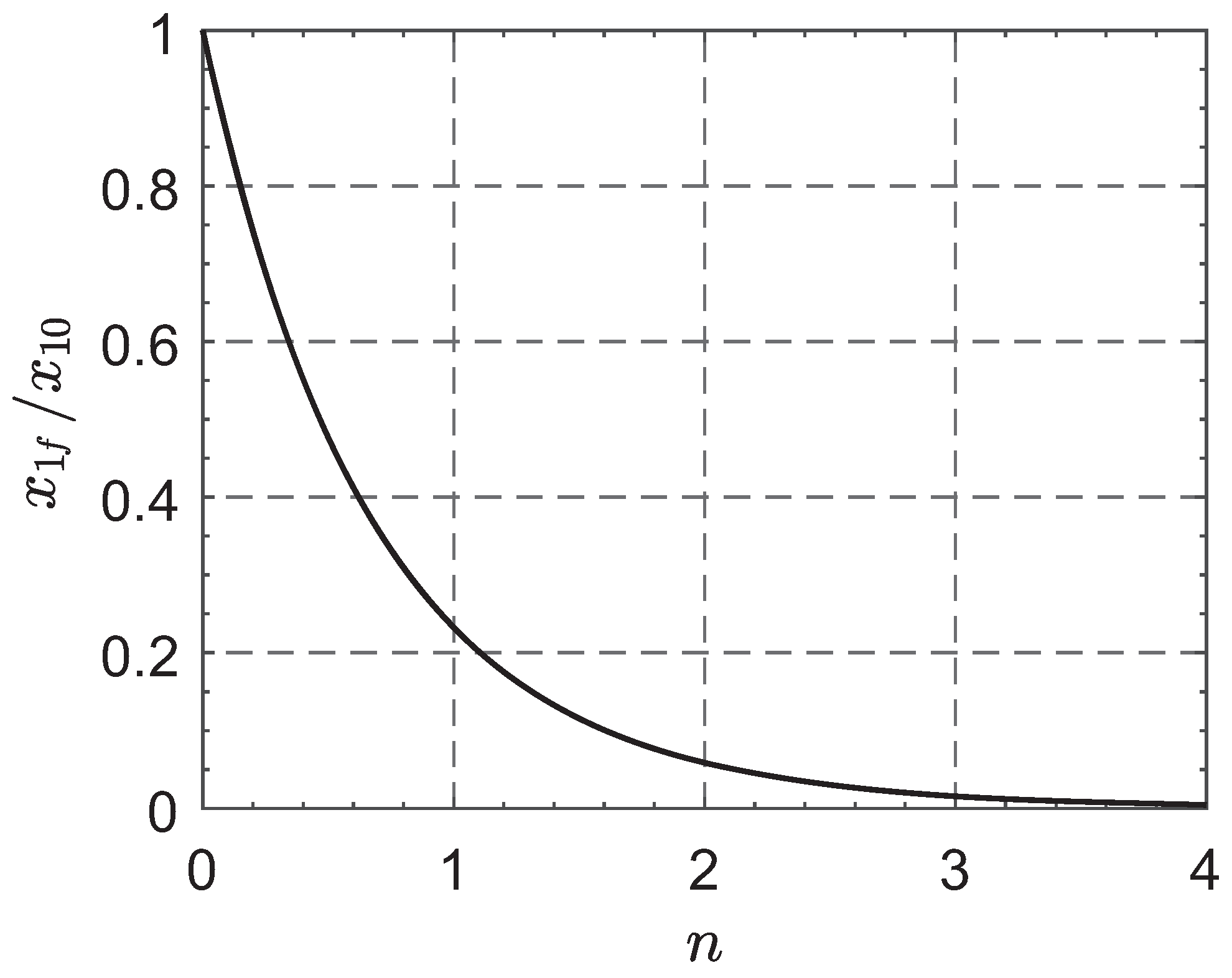
The control law described by Equations (26) and (29) takes a simpler form in the case of an unperturbed system, which allows some useful analytical relationships to be found in such a simplified mission scenario. Accordingly, in this section, we analyze the evolution of the tracking errors and address the control law design problem with the significant assumption that $Z_r=Z_t=0$. In this simplified case, Equations (28) and (31) become

$$\begin{array}{c}\hfill s^{\prime }=-K\mathrm{sign}\left(s\right)\end{array}$$

(40)

$$\begin{array}{c}\hfill x_3^{\prime }=-c\mathrm{sign}\left(x_3\right)\end{array}$$

(41)

This means that in the absence of perturbative terms, the value of s (or $x_3$) approaches zero linearly with respect to $\tau$, and once the sliding surface $s=0$ (or $x_3=0$) is reached for the first time, the term s (or $x_3$) remains stationary at zero. When Equations (40) and (41) are integrated with respect to the dimensionless time $\tau$, one obtains the $\tau$-variations of s and $x_3$ before reaching the sliding surfaces $s=0$ and $x_3=0$, respectively. The result is

$$\begin{array}{cc}\hfill s\left(\tau \right)& =s_0-\mathrm{sign}\left(s_0\right)K\tau \hfill \end{array}$$

(42)

$$\begin{array}{cc}\hfill x_3\left(\tau \right)& =x_{3_0}-\mathrm{sign}\left(x_{3_0}\right)c\tau \hfill \end{array}$$

(43)

where $s_0\triangleq s\left({\tau }_0\right)$ can be written, according to Equations (18) and (22), as

$$s_0=x_{2_0}+\lambda x_{1_0}\equiv \lambda \left(1-\rho \right)$$

(44)

while $x_{3_0}$ is given by the last of Equation (18) as a function of $\rho$. Note that $\{K,c\}$ represent a sort of approach speed to the two sliding surfaces.

The value of $\tau$ at which the system reaches the sliding surface $s=0$ (i.e., $\tau ={\tau }_s$) or the sliding surface $x_3=0$ (i.e., $\tau ={\tau }_{x_3}$) can be expressed in a compact form using Equations (42) and (43). In fact, enforcing the condition $s=0$ in Equation (42) gives

$$s_0-\mathrm{sign}\left(s_0\right)K{\tau }_s\triangleq 0$$

(45)

from which

$${\tau }_s\triangleq {\displaystyle \frac{\lambda |1-\rho |}{K}}$$

(46)

while the condition $x_3=0$ in Equation (43) gives

$$x_{3_0}-\mathrm{sign}\left(x_{3_0}\right)c{\tau }_{x_3}\triangleq 0$$

(47)

from which

$${\tau }_{x_3}\triangleq {\displaystyle \frac{|1-1/\sqrt{\rho }|}{c}}$$

(48)

The value of ${\tau }_{x_3}$ may be written as a function of ${\tau }_s$ in a more convenient way by introducing the dimensionless parameter $\beta >0$ such that

$${\tau }_{x_3}=\beta {\tau }_s$$

(49)

Observing that $\beta$ is a redundant parameter, it may be used in place of c, which can be expressed as a function of $\{K,\lambda ,\beta ,\rho \}$ as

$$c\triangleq {\displaystyle \frac{K\left(1-1/\sqrt{\rho }\right)}{\lambda \beta \left(\rho -1\right)}}$$

(50)

4.1. The $\tau$-Variation of Tracking Errors and Controls

The $\tau$-variation of the tracking errors is now calculated, thus allowing the expressions of $u_r$ and $u_t$ to be determined through Equations (26) and (29) by simply setting $\delta =K$ and $\gamma =c$. To that end, the differential equation governing the $\tau$-evolution of $x_1$ is found by substituting Equations (11) and (22) into Equation (42) and bearing in mind Equations (44)–(46), viz.

$$x_1^{\prime }+\lambda x_1=\left\{\begin{array}{c}\lambda \left(1-\rho \right)-\mathrm{sign}\left(1-\rho \right)K\tau \mathrm{if}\tau <{\tau }_s\hfill \\ 0\mathrm{otherwise}\hfill \end{array}\right.$$

(51)

Integrating Equation (51) with respect to $\tau$ with the initial condition $x_1\left({\tau }_0\right)=1-\rho$ (see Equation (18)) gives the $\tau$-variation of $x_1$, that is,

$${\displaystyle \frac{x_1\left(\tau \right)}{\mathrm{sign}\left(1-\rho \right)}}=\left\{\begin{array}{c}{\displaystyle \frac{K}{{\lambda }^2}}\left(1-e^{-\lambda \tau }-\lambda \tau \right)+1-\rho \mathrm{if}\tau <{\tau }_s\hfill \\ {\displaystyle \frac{K}{{\lambda }^2}}\left(1-e^{-\lambda {\tau }_s}\right)e^{-\lambda \left(\tau -{\tau }_s\right)}\mathrm{otherwise}\hfill \end{array}\right.$$

(52)

The $\tau$-variation of $x_2$ is instead obtained by deriving Equation (52) with respect to $\tau$ (see Equation (11)), that is,

$${\displaystyle \frac{x_2\left(\tau \right)}{\mathrm{sign}\left(1-\rho \right)}}=\left\{\begin{array}{c}{\displaystyle \frac{K}{\lambda }}\left(e^{-\lambda \tau }-1\right)\mathrm{if}\tau <{\tau }_s\hfill \\ {\displaystyle \frac{K}{\lambda }}\left(e^{-\lambda {\tau }_s}-1\right)e^{-\lambda \left(\tau -{\tau }_s\right)}\mathrm{otherwise}\hfill \end{array}\right.$$

(53)

Finally, the $\tau$-variation of $x_3$ is governed by the differential equation

$$x_3^{\prime }=\left\{\begin{array}{c}-c\mathrm{sign}\left(x_3\right)\mathrm{if}\tau <\beta {\tau }_s\hfill \\ 0\mathrm{otherwise}\hfill \end{array}\right.$$

(54)

which must be solved recalling the initial condition $x_3\left({\tau }_0\right)=1-1/\sqrt{\rho }$ (see Equation (18)), and the result is

$${\displaystyle \frac{x_3\left(\tau \right)}{\mathrm{sign}\left(1-1/\sqrt{\rho }\right)}}=\left\{\begin{array}{c}|1-1/\sqrt{\rho }|-c\tau \mathrm{if}\tau <\beta {\tau }_s\hfill \\ 0\mathrm{otherwise}\hfill \end{array}\right.$$

(55)

Note that in the absence of perturbative terms, the maximum values of $|x_1|$ and $|x_3|$ occur when $\tau ={\tau }_0$, that is,

$$\begin{array}{cc}\hfill max\left(|x_1|\right)& =|x_{1_0}|\equiv |1-\rho |\hfill \end{array}$$

(56)

$$\begin{array}{cc}\hfill max\left(|x_3|\right)& =|x_{3_0}|\equiv |1-1/\sqrt{\rho }|\hfill \end{array}$$

(57)

while the maximum value of $|x_2|$ (which corresponds to the maximum of $|v_r|$) is reached when $\tau ={\tau }_s$, viz.

$$max\left(|x_2|\right)={\displaystyle \frac{K}{\lambda }}|e^{-\lambda {\tau }_s}-1|$$

(58)

The dimensionless propulsive acceleration components $\{u_r,u_t\}$ in absence of perturbative terms are simply obtained by substituting Equations (52), (53), and (55) into Equations (26) and (29) and setting $\delta =K$ and $\gamma =c$. Those expressions, which are here omitted for the sake of conciseness, change according to whether $\beta <1$, $\beta =1$, or $\beta >1$. In particular, $u_r$ exhibits a discontinuity equal to $K\mathrm{sign}\left(1-\rho \right)$ when $\tau ={\tau }_s$, whereas $u_t$ exhibits a discontinuity equal to $c\mathrm{sign}\left(1-\sqrt{\rho }\right)$ when $\tau =\beta {\tau }_s$. Accordingly, if $\beta \ne 1$, the profile of the magnitude $u\triangleq \sqrt{u_r^2+u_t^2}$ has two discontinuities (one at $\tau ={\tau }_s$, the other at $\tau =\beta {\tau }_s$). Otherwise (i.e., when $\beta =1$), the profile of u presents a single discontinuity at $\tau ={\tau }_s$.

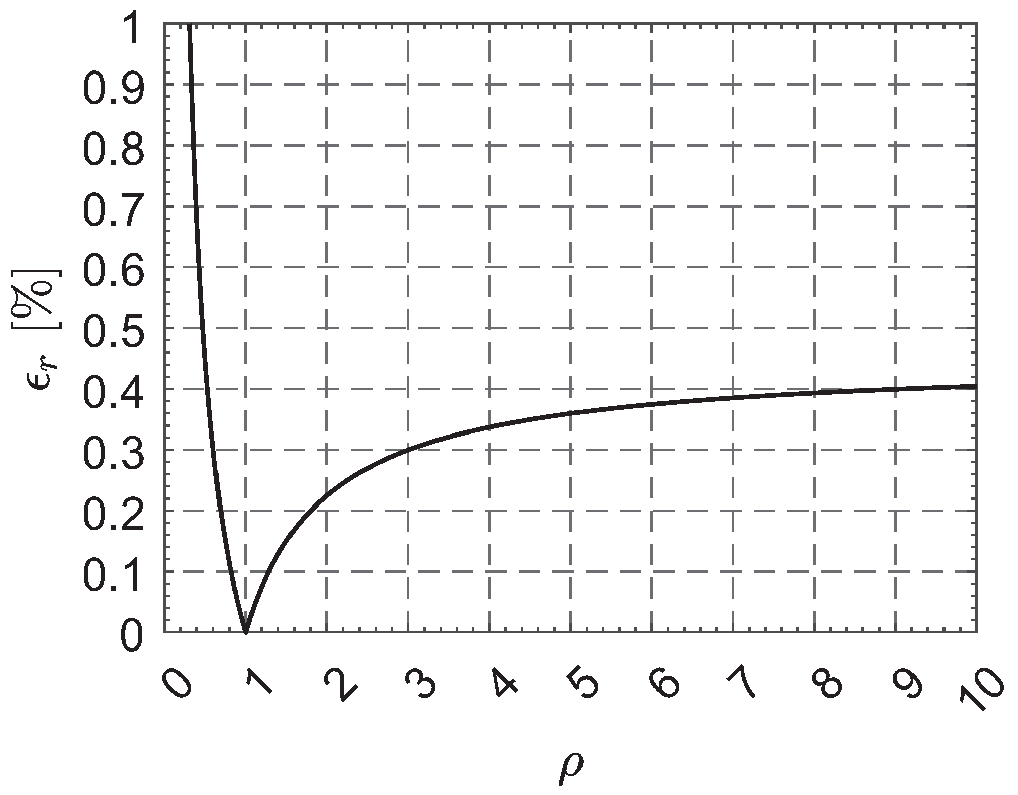
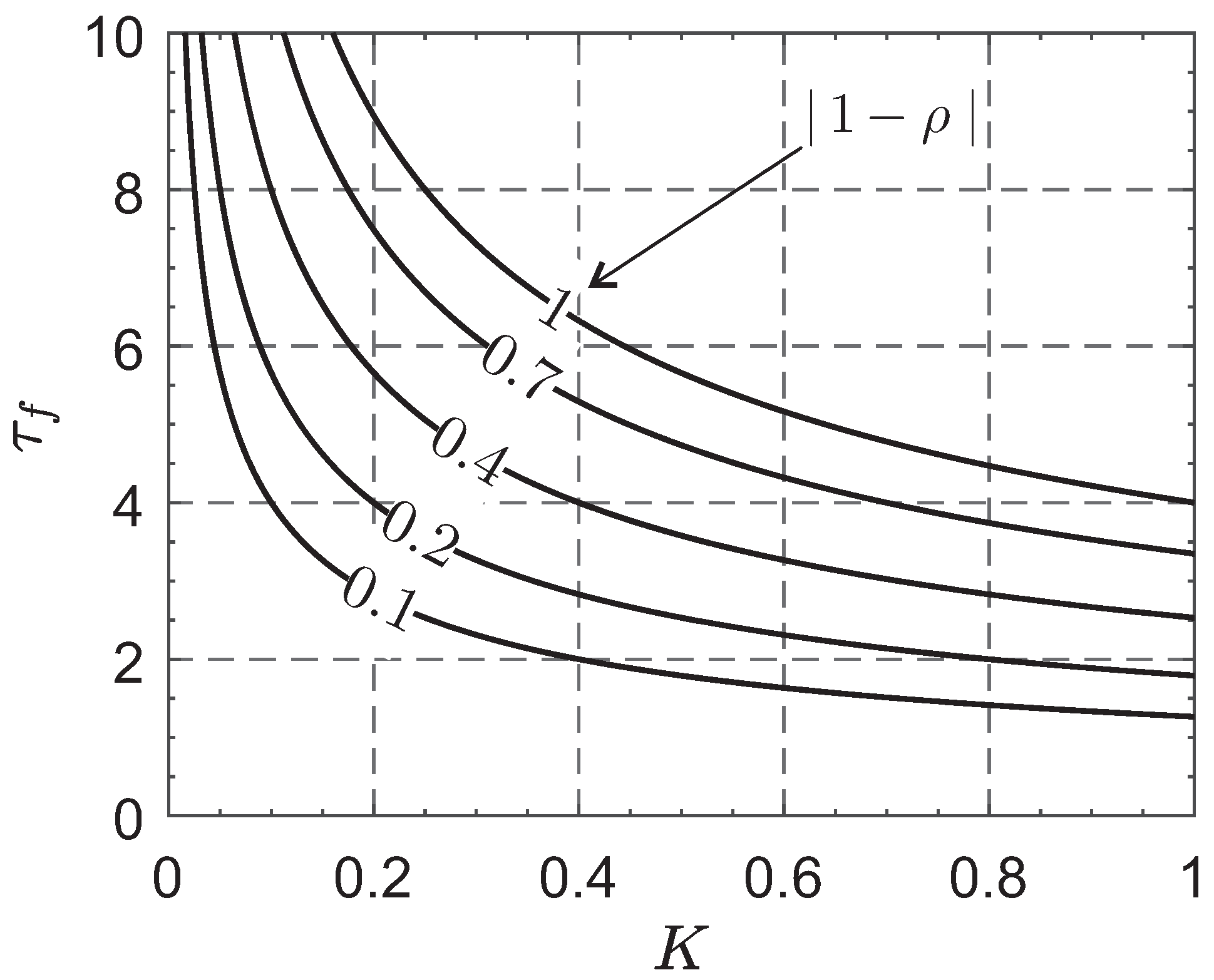
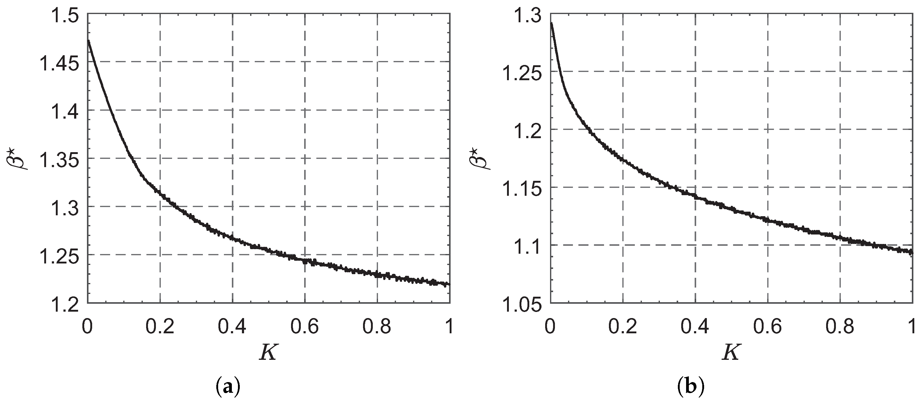
4.2. Control Parameter Selection

For a given value of $\rho$, the design of the sliding mode control law amounts to selecting the values of the triplet $\{K,\lambda ,\beta \}$. The previous expressions allow the flight time and the total velocity change to be determined and the dimensionless parameters in the control law to be established, according to arbitrary criteria. More precisely, when the spacecraft orbital dynamics is unaffected by external disturbances or model uncertainties, the dimensionless flight time ${\tau }_f$ and the total velocity change $\Delta v$ can be calculated with analytical expressions or graphic plots that only depend on the design parameters $\{K,\lambda ,\beta \}$.

For example, the value of ${\tau }_f$ can be obtained by assuming that the orbit transfer terminates when the tracking errors $x_1$ and $x_2$ are sufficiently close to zero. To that end, the value of ${\tau }_f$ is defined as the instant at which the exponent $\lambda (\tau -{\tau }_s)$ in Equations (52) and (53) satisfies the equality $\lambda ({\tau }_f-{\tau }_s)=n$, for an assigned value of $n\in {\mathbb{R}}^{+}$. In this context, using Equation (46), one obtains

$${\tau }_f={\tau }_s+{\displaystyle \frac{n}{\lambda }}\equiv {\displaystyle \frac{\lambda |1-\rho |}{K}}+{\displaystyle \frac{n}{\lambda }}$$

(59)

Note that ${\tau }_f$ can be minimized with respect to $\lambda$ by enforcing the necessary condition

$${\displaystyle \frac{\partial {\tau }_f}{\partial \lambda }}=0$$

(60)

in Equation (59), from which

$$\lambda ={\lambda }^{★}\triangleq \sqrt{{\displaystyle \frac{nK}{|1-\rho |}}}$$

(61)

so that, by assuming $\lambda ={\lambda }^{★}$, the expression of the dimensionless flight time becomes

$${\tau }_f=2\sqrt{{\displaystyle \frac{n|1-\rho |}{K}}}\equiv 2{\tau }_s{|}_{\lambda ={\lambda }^{★}}$$

(62)

A suitable value of n may be chosen by evaluating the tracking error $x_1$ at the final time $\tau ={\tau }_f$, that is,

$$x_1\left({\tau }_f\right)={\displaystyle \frac{e^{-n}\left(1-e^{-n}\right)}{n}}{x}_{1_0}$$

(63)

Figure 2, which describes the variation of $x_1\left({\tau }_f\right)/x_{1_0}$ with n when $\lambda ={\lambda }^{★}$, shows that a value of $n=4$ (when $x_1\left({\tau }_f\right)/x_{1_0}\simeq 0.0045$) is reasonable from a practical point of view. In fact, the percentage error in orbital radius, that is, the function

$${ϵ}_r\triangleq {\displaystyle \frac{|r\left(t_f\right)-r_f|}{r_f}}\times 100\simeq {\displaystyle \frac{0.45|1-\rho |}{\rho }}$$

(64)

is less than $1\%$ when $n=4$ and $\rho >0.310$; see Figure 3. Therefore, it is assumed that $n=4$ in the rest of the paper.

According to Equations (61) and (62), the expressions of ${\lambda }^{★}$ and ${\tau }_f$ when $n=4$ become

$$\begin{array}{cc}\hfill {\lambda }^{★}& =2\sqrt{{\displaystyle \frac{K}{|1-\rho |}}}\hfill \end{array}$$

(65)

$$\begin{array}{cc}\hfill {\tau }_f& =4\sqrt{{\displaystyle \frac{|1-\rho |}{K}}}\equiv {\displaystyle \frac{8}{{\lambda }^{★}}}\hfill \end{array}$$

(66)

Note that Equation (66) relates the flight time ${\tau }_f$ to the value of $\lambda$ necessary to minimize the flight time for fixed values of K and $\rho$. Such a value of $\lambda$ is a function of K and $\rho$, as described by Equation (65). This means that for given values of $\rho$ and ${\tau }_f$, $\lambda$ can be chosen by reversing Equation (66), that is, by setting $\lambda ={\lambda }^{★}\equiv 8/{\tau }_f$. In this case, the value of K is related to $\rho$ and $\lambda$ (or to $\rho$ and ${\tau }_f$) through Equation (65), and Figure 4 shows the variation in ${\tau }_f$ with K and $\rho$.

The value of $\beta$ can be chosen with the aid of another parameter that usually determines the transfer performance. More precisely, $\beta$ may be related to the total velocity change $\Delta v$ of the transfer, defined as

$$\Delta v\triangleq {\int }_0^{{\tau }_f}u\mathrm{d}\tau$$

(67)

Note that $\beta \in (0,2]$, since $\beta \to 0$ (or $\beta =2$) means that the sliding surface $x_3=0$ is reached at the beginning (or at the end) of the transfer; see Equations (49) and (62). Figure 5 shows the values of $\beta$ (referred to as ${\beta }^{★}$) that minimize the total velocity change when $\lambda ={\lambda }^{★}$, $n=4$, and $\rho =\{0.723,1.524\}$ (the same values of $\rho$ that will be used for some numerical applications of the proposed control law) as a function of $K\in (0,1]$. In fact, K corresponds to the magnitude of the discontinuity of $u_r$ when $\tau ={\tau }_s$ (see Section 4.1), and a value of K greater than 1 would imply a discontinuity of $|a_r|$ greater than the gravitational acceleration on the parking orbit. Figure 6, instead, shows the variation in $\Delta v$ with K when $\lambda ={\lambda }^{★}$, $n=4$, and $\beta ={\beta }^{★}$. Note that the function ${\Delta v|}_{\beta ={\beta }^{★}}\left(K\right)$ exhibits a global minimum. When $\rho =0.723$, such a minimum is reached when $K\simeq 0.097$ and the corresponding values of $\Delta v$ and ${\beta }^{★}$ are $\Delta v\simeq 0.357$ and ${\beta }^{★}\simeq 1.368$, respectively. If, instead, $\rho =1.524$, such a minimum is reached when $K\simeq 0.032$ and the corresponding values of $\Delta v$ and ${\beta }^{★}$ are $\Delta v\simeq 0.324$ and ${\beta }^{★}\simeq 1.242$, respectively.

In essence, the design of the control law only requires the choice of the single parameter K. For example, we have already seen that a value of K may be determined using Equations (65) and (66) by fixing the total flight time ${\tau }_f$, or using Figure 6 by looking for the value of K that minimizes the function ${\Delta v|}_{\beta ={\beta }^{★}}\left(K\right)$, so that K may be thought of as sort of trade-off parameter, as discussed in the next section.

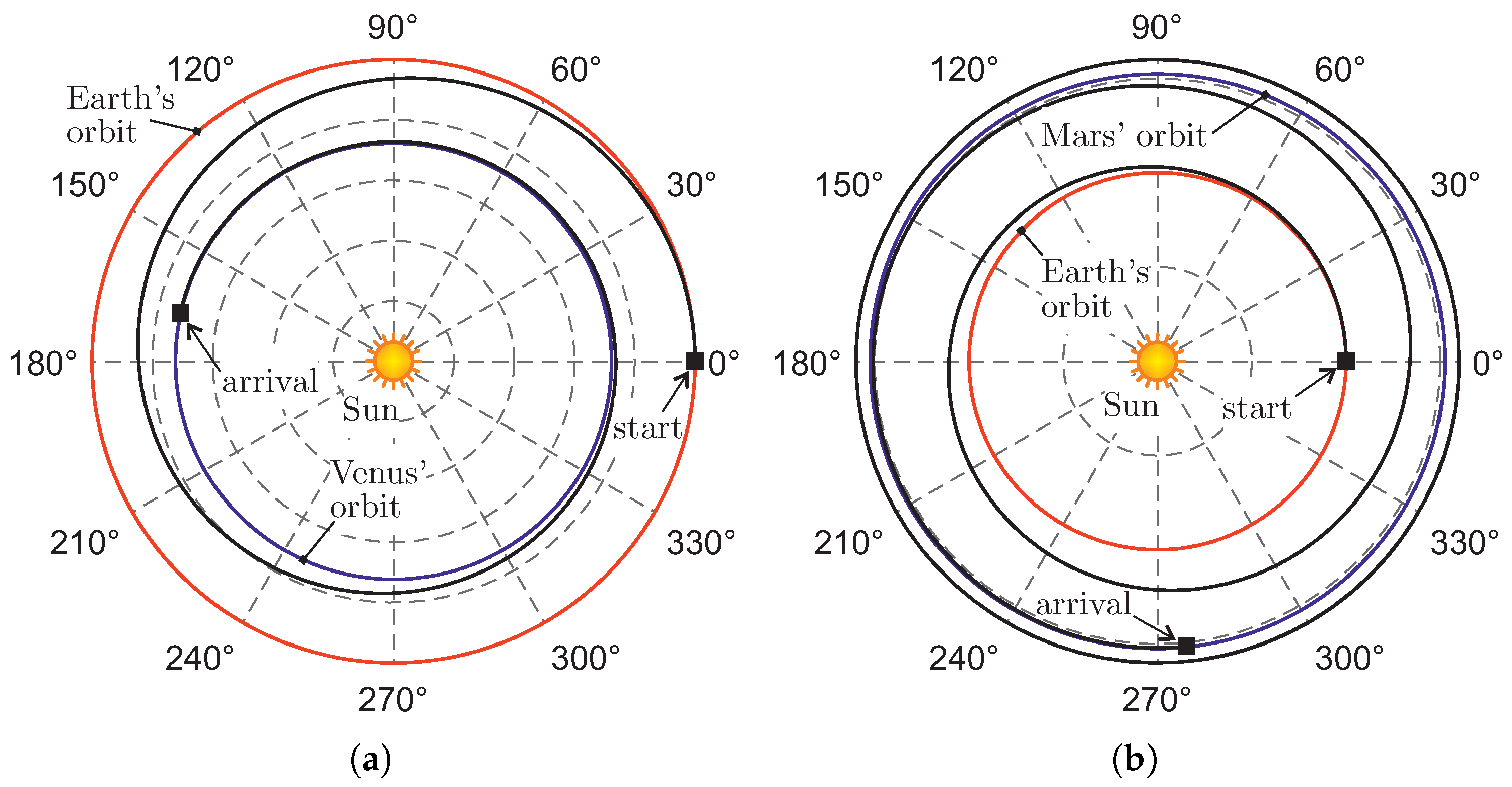
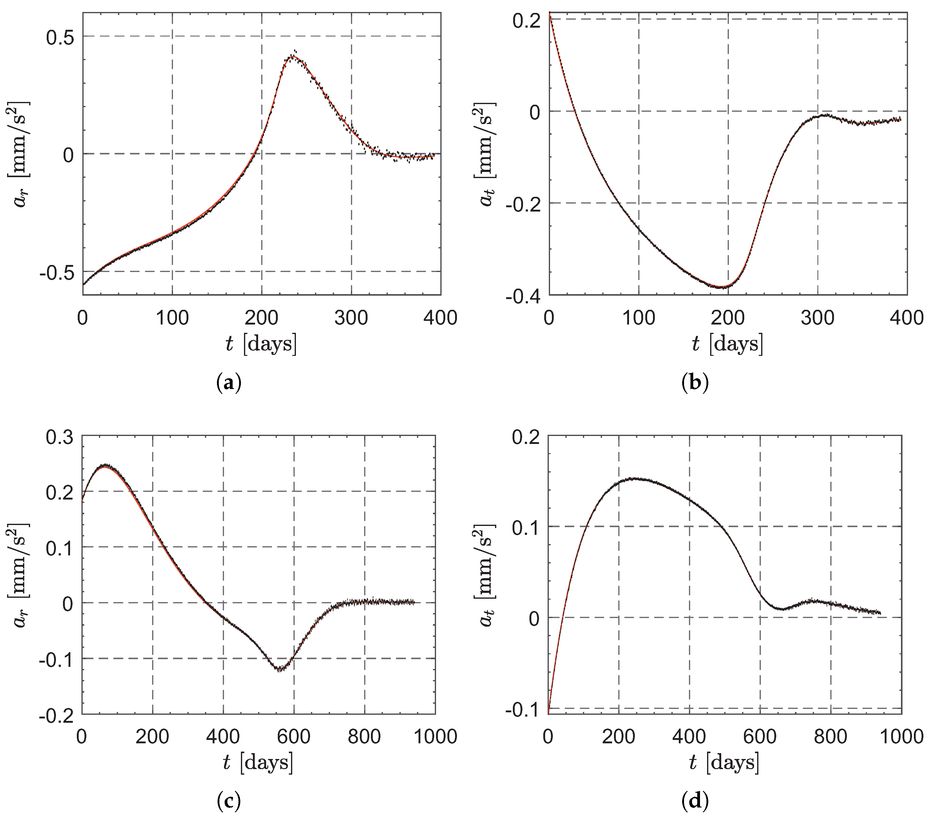
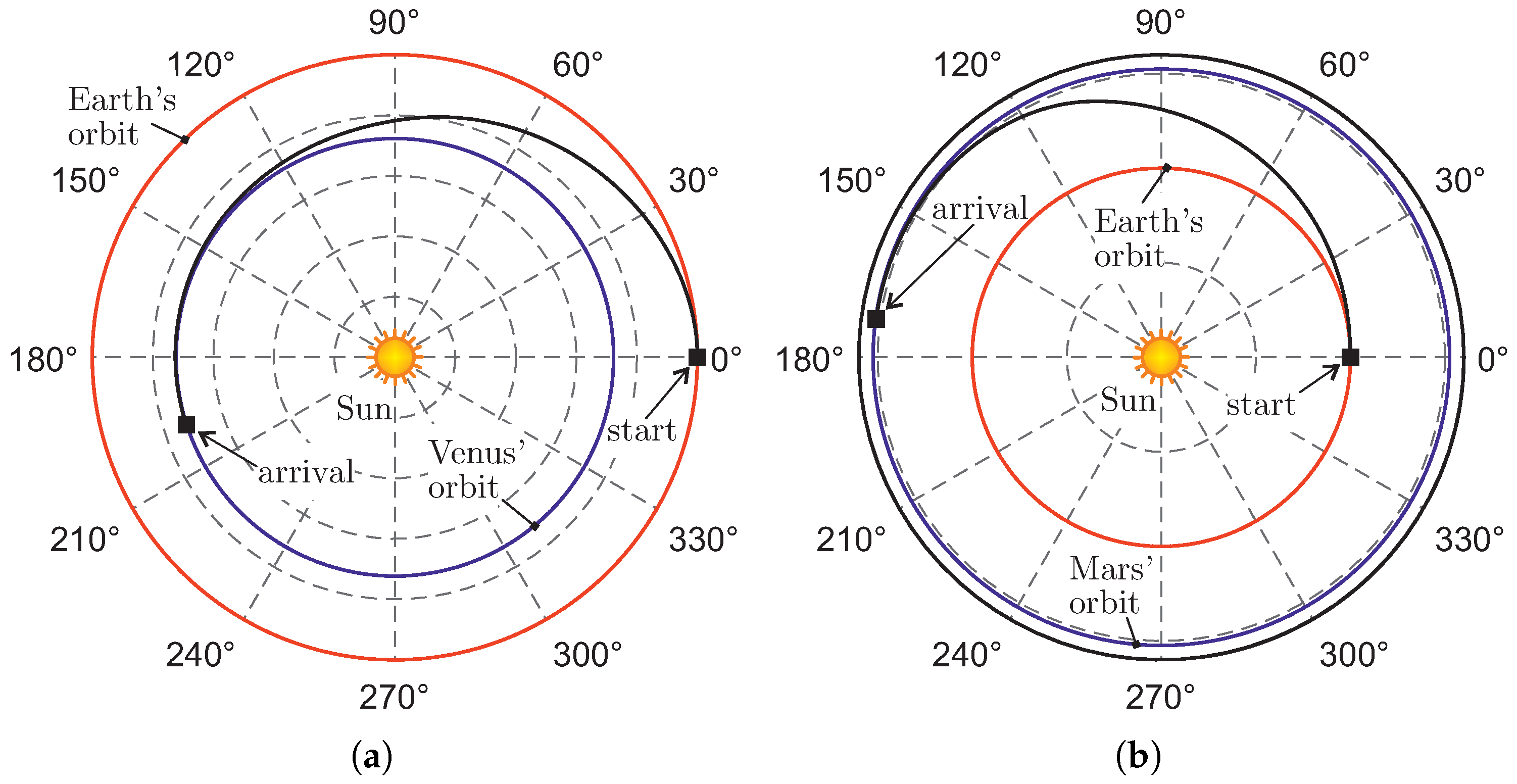
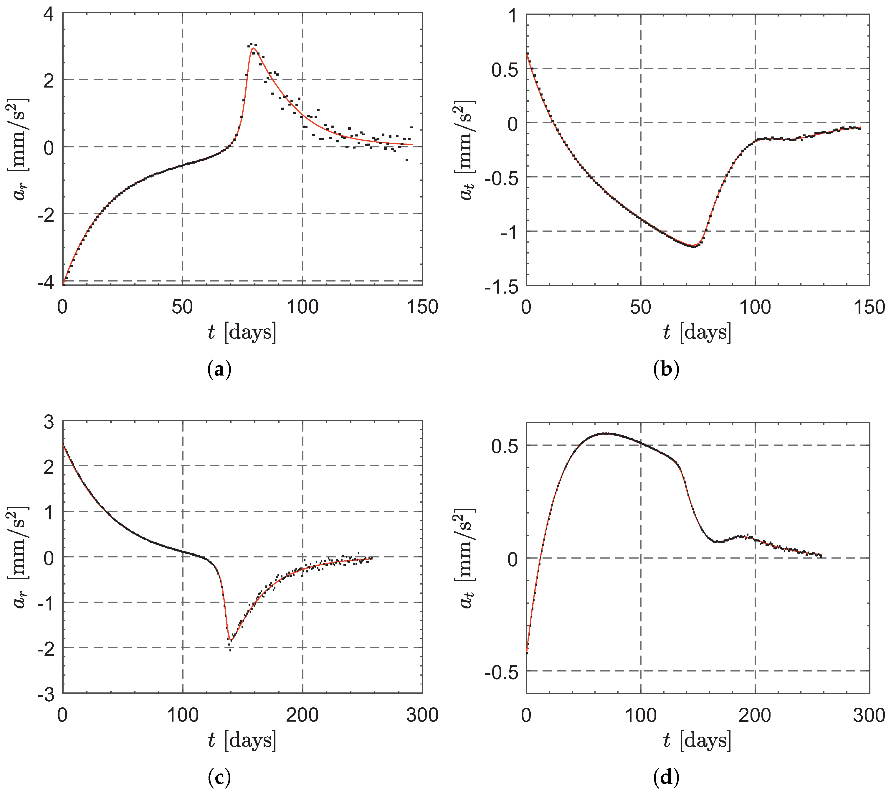
5. Numerical Simulations and Mission Application

The proposed control strategy is now used to analyze two classical circle-to-circle interplanetary transfers. In particular, the radius of the circular parking orbit is $r_0=r_{\oplus }\triangleq 1\mathrm{au}$, which is consistent with a spacecraft that leaves the Earth’s sphere of influence using a parabolic escape trajectory, with the simplifying assumption that the Earth’s heliocentric orbit is circular. The radii of the target orbits are $r_f=\{0.723,1.524\}\mathrm{au}$, so the analyzed mission scenarios describe simplified ephemeris-free Earth–Venus and Earth–Mars orbit transfers.

Bearing in mind Equations (32)–(34), it is assumed that (i) the sensors measure the states once per day; (ii) ${\sigma }_1={\sigma }_2={\sigma }_3={10}^{-4}$, which means that the measurement error in $\{x_1,x_2,x_3\}$ is less than $0.01\%$ with a probability of $68.3\%$; and (iii) the sigmoid-like function $\mathcal{S}=\mathcal{S}\left(x\right)$ of Equation (35) is obtained with $\kappa ={10}^{-2}$. Although the numerical simulations consider measurement errors, low-frequency sampling, and the approximation of the signum function with the sigmoid-like function, the parameters used in the control law can be those found in Section 4.2 thanks to the robustness of the proposed approach.

For example, assume that $\lambda ={\lambda }^{★}$, $n=4$, $\beta ={\beta }^{★}$, and select K such that ${\Delta v|}_{\beta ={\beta }^{★}}$ is minimized (the corresponding value of K will be referred to as $K_v$), so that according to Figure 6, one has $K_v\simeq 0.0969$ (or $K_v\simeq 0.0320$) when $\rho =0.723$ (or $\rho =1.524$). The numerical simulations give a flight time of about $394\mathrm{days}$ (or $949\mathrm{days}$) in the Earth–Venus (or Earth–Mars) mission scenario. Moreover, Figure 7 shows the corresponding (two-dimensional) heliocentric trajectories, while Figure 8 shows the time-variations of the propulsive acceleration components $\{a_r,a_t\}$. In particular, each black dot in Figure 8 corresponds to one day (i.e., to the sampling period of the states), while the red lines show the propulsive acceleration components in case of ideal sensors and actuators (that is, when only the approximation of the signum function with the sigmoid-like function is taken into account).

A second case considered in the simulations is when the flight time is assigned, $\lambda ={\lambda }^{★}\equiv 8/{\tau }_f$, $n=4$, and $\beta ={\beta }^{★}$. For example, by assuming that the transfer time coincides with the Hohmann transfer one, the values of ${\tau }_f$ become

$${\tau }_f={\tau }_H\triangleq \pi \sqrt{{\displaystyle \frac{{\left(1+\rho \right)}^3}{8}}}\simeq \left\{\begin{array}{cc}2.512\hfill & \mathrm{if}\rho =0.723\hfill \\ 4.454\hfill & \mathrm{if}\rho =1.524\hfill \end{array}\right.$$

(68)

which correspond to a flight time of $146\mathrm{days}$ in the Earth–Venus scenario and to $259\mathrm{days}$ in Earth–Mars case. In these cases, by using Equation (66), the values of ${\lambda }^{★}$ and K, respectively referred to as ${\lambda }_H^{★}$ and $K_H$, are given by

$$\begin{array}{cc}\hfill {\lambda }_H^{★}& ={\displaystyle \frac{8}{{\tau }_H}}\simeq \left\{\begin{array}{cc}3.185\hfill & \mathrm{if}\rho =0.723\hfill \\ 1.796\hfill & \mathrm{if}\rho =1.524\hfill \end{array}\right.\hfill \end{array}$$

(69)

$$\begin{array}{cc}\hfill K_H& =|1-\rho |{\left({\displaystyle \frac{{\lambda }_H^{★}}{2}}\right)}^2\simeq \left\{\begin{array}{cc}0.702\hfill & \mathrm{if}\rho =0.723\hfill \\ 0.423\hfill & \mathrm{if}\rho =1.524\hfill \end{array}\right.\hfill \end{array}$$

(70)

while the values of ${\beta }^{★}$ are chosen by using Figure 5 to minimize the total velocity change, viz.

$${\beta }^{★}\simeq \left\{\begin{array}{cc}1.234\hfill & \mathrm{if}\rho =0.723\hfill \\ 1.138\hfill & \mathrm{if}\rho =1.524\hfill \end{array}\right.$$

(71)

In this context, Figure 9 shows the interplanetary transfer trajectories, while Figure 10 collects the time-variations of the propulsive acceleration components $\{a_r,a_t\}$ for the two mission scenarios.

Once the control parameters are selected and the transfer trajectory is obtained, it is possible to evaluate the time-variation of the magnitude of the propulsive acceleration vector $a\triangleq \sqrt{a_r^2+a_t^2}$ during the transfer. Figure 11 shows the values of a as a function of time in the four cases previously described. The curves depicted in that figure can be used to evaluate, a posteriori, the feasibility of the obtained transfer trajectory according to the actual thruster installed on board. In particular, Figure 11a (or Figure 11b) indicates that the maximum value of a during an Earth-Venus (or Earth-Mars) transfer with $K=K_v$ is about $0.6\mathrm{mm}/{\mathrm{s}}^2$ (or $0.25\mathrm{mm}/{\mathrm{s}}^2$), while Figure 11c (or Figure 11d) shows that the maximum value of a is roughly $4.2\mathrm{mm}/{\mathrm{s}}^2$ (or $2.5\mathrm{mm}/{\mathrm{s}}^2$) for an Earth–Venus (or Earth–Mars) case when ${\tau }_f={\tau }_H$. Therefore, if, for example, the installed thruster gives a maximum propulsive acceleration of $0.3\mathrm{mm}/{\mathrm{s}}^2$, when $K=K_v$, one concludes that the transfer trajectory obtained in the Earth–Mars case can be theoretically flown, while the result in the Earth–Venus scenario gives a trajectory that violates the propulsive constraint. In the latter case (that is, in the Earth–Venus scenario with $K=K_v$), the designer could suitably change the control law parameters in order to reduce the maximum value of a reached during the transfer. For example, when $K=0.03$ and $\beta =1.48$, the maximum value of a reduces to about $0.29\mathrm{mm}/{\mathrm{s}}^2$, while the flight time rises to roughly $1413\mathrm{days}$.

The previous results may be easily extended to trade-off solutions between the flight time and the total velocity change necessary to complete the transfer. Recall in fact that, for a given value of $\rho$, the flight time is a function of K according to Equation (66), while the total velocity change depends on K as Figure 6 shows. Therefore, it is possible to plot the value of ${\Delta v|}_{\beta ={\beta }^{★}}$ as a function of ${\tau }_f$. The results are shown in Figure 12, where K ranges within the interval $[K_v,1]$ and the black squares correspond to the cases in which the flight time equals the Hohmann transfer time. Figure 12 represents a simple and effective means to identify reasonable compromise solutions, which are useful in a preliminary analysis of the trajectory design.

6. Conclusions

In this paper, we have investigated the capabilities of a sliding mode control technique of rapidly generating a possible trajectory for a spacecraft in a typical circle-to-circle orbit transfer mission scenario. Such a control strategy, which is a robust technique usually used for controlling nonlinear systems affected by disturbances, has been employed here to obtain simple mathematical relations and graphs that allow the designer to estimate the (possible) transfer trajectory characteristics as a function of few tuning parameters.

The proposed approach has shown to be effective even in the presence of bounded disturbances due to measurement errors and low-frequency sampling. It may be effectively employed in an early phase of trajectory planning, that is, just before the usual refinement phase that provides the nominal spacecraft trajectory to be tracked during the transfer. In particular, the discussed approach has the scope of reducing the complexity of the mathematical model and the computational cost required to obtain a possible solution to the transfer problem. However, rather strong simplifying assumptions have been adopted, such as the use of a sort of ideal thruster with a freely steerable thrust vector, or the definition of the error in terms of the desired states. A more accurate estimate of the actual propulsive acceleration profile can be obtained by relaxing some of those assumption. This aspect represents the natural extension of this work.

References

1. Slotine, J.J.E.; Li, W. Applied Nonlinear Control; Prentice-Hall: Englewood Cliffs, NJ, USA, 1991; Chapter 7; pp. 276–310. [Google Scholar]
2. Gambhire, S.J.; Kishore, D.R.; Londhe, P.S.; Pawar, S.N. Review of sliding mode based control techniques for control system applications. Int. J. Dyn. Control 2020, 9, 363–378. [Google Scholar] [CrossRef]
3. Qureshi, M.S.; Das, S.; Swarnkar, P.; Gupta, S. Design and Implementation of Sliding Mode Control for Uncertain Systems. Mater. Today Proc. 2018, 5, 4299–4308. [Google Scholar] [CrossRef]
4. Hung, J.; Gao, W.; Hung, J. Variable structure control: A survey. IEEE Trans. Ind. Electron. 1993, 40, 2–22. [Google Scholar] [CrossRef]
5. Utkin, V. Sliding mode control design principles and applications to electric drives. IEEE Trans. Ind. Electron. 1993, 40, 23–36. [Google Scholar] [CrossRef]
6. Chen, T.; Shan, J.; Wen, H.; Xu, S. Review of attitude consensus of multiple spacecraft. Astrodynamics 2022, 6, 329–356. [Google Scholar] [CrossRef]
7. Wu, B.; Wang, D.; Poh, E.K. Decentralized sliding-mode control for spacecraft attitude synchronization under actuator failures. Acta Astronaut. 2014, 105, 333–343. [Google Scholar] [CrossRef]
8. Massey, T.; Shtessel, Y. Continuous Traditional and High-Order Sliding Modes for Satellite Formation Control. J. Guid. Control Dyn. 2005, 28, 826–831. [Google Scholar] [CrossRef]
9. Ma, Z.; Sun, G. Adaptive sliding mode control of tethered satellite deployment with input limitation. Acta Astronaut. 2016, 127, 67–75. [Google Scholar] [CrossRef]
10. Liu, S.; Huo, W. Terminal sliding mode control for space rendezvous and docking. In Proceedings of the International Conference on Computational Intelligence and Communication Networks (CICN), Jabalpur, India, 12–14 December 2015. [Google Scholar] [CrossRef]
11. Dong, J.; Li, C.; Jiang, B.; Sun, Y. Fixed-time nonsingular terminal sliding mode control for spacecraft rendezvous. In Proceedings of the 29th Chinese Control and Decision Conference (CCDC), Chongqing, China, 28–30 May 2017. [Google Scholar] [CrossRef]
12. Capello, E.; Punta, E.; Dabbene, F.; Guglieri, G.; Tempo, R. Sliding-mode control strategies for rendezvous and docking maneuvers. J. Guid. Control Dyn. 2017, 40, 1481–1488. [Google Scholar] [CrossRef]
13. Kasaeian, S.A.; Assadian, N.; Ebrahimi, M. Sliding mode predictive guidance for terminal rendezvous in eccentric orbits. Acta Astronaut. 2017, 140, 142–155. [Google Scholar] [CrossRef]
14. Li, Q.; Yuan, J.; Wang, H. Sliding mode control for autonomous spacecraft rendezvous with collision avoidance. Acta Astronaut. 2018, 151, 743–751. [Google Scholar] [CrossRef]
15. Bassetto, M.; Niccolai, L.; Boni, L.; Mengali, G.; Quarta, A.A.; Circi, C.; Pizzurro, S.; Pizzarelli, M.; Pellegrini, R.C.; Cavallini, E. Sliding mode control for attitude maneuvers of Helianthus solar sail. Acta Astronaut. 2022, 198, 100–110. [Google Scholar] [CrossRef]
16. Aliasi, G.; Mengali, G.; Quarta, A.A. Artificial Lagrange points for solar sail with electrochromic material panels. J. Guid. Control Dyn. 2013, 36, 1544–1550. [Google Scholar] [CrossRef]
17. Boni, L.; Bassetto, M.; Niccolai, L.; Mengali, G.; Quarta, A.A.; Circi, C.; Pellegrini, R.C.; Cavallini, E. Structural response of Helianthus solar sail during attitude maneuvers. Aerosp. Sci. Technol. 2023, 133, 108152. [Google Scholar] [CrossRef]
18. Quarta, A.A.; Mengali, G. Solar sail orbit raising with electro-optically controlled diffractive film. Appl. Sci. 2023, 13, 7078. [Google Scholar] [CrossRef]
19. Wang, X.; Roy, S.; Farì, S.; Baldi, S. Adaptive Vector Field Guidance Without a Priori Knowledge of Course Dynamics and Wind. IEEE/ASME Trans. Mechatron. 2022, 27, 4597–4607. [Google Scholar] [CrossRef]
20. Bai, Y.; Yan, T.; Fu, W.; Li, T.; Huang, J. Robust Adaptive Composite Learning Integrated Guidance and Control for Skid-to-Turn Interceptors Subjected to Multiple Uncertainties and Constraints. Actuators 2023, 12, 243. [Google Scholar] [CrossRef]
21. Feng, C.; Chen, W.; Shao, M.; Ni, S. Trajectory Tracking and Adaptive Fuzzy Vibration Control of Multilink Space Manipulators with Experimental Validation. Actuators 2023, 12, 138. [Google Scholar] [CrossRef]
22. Xie, R.; Dempster, A.G. An on-line deep learning framework for low-thrust trajectory optimisation. Aerosp. Sci. Technol. 2021, 118, 107002. [Google Scholar] [CrossRef]
23. Peloni, A.; Rao, A.V.; Ceriotti, M. Automated Trajectory Optimizer for Solar Sailing (ATOSS). Aerosp. Sci. Technol. 2018, 72, 465–475. [Google Scholar] [CrossRef]
24. Patterson, M.J.; Benson, S.W. NEXT ion propulsion system development status and performance. In Proceedings of the 43rd AIAA/ASME/SAE/ASEE Joint Propulsion Conference and Exhibit, Cincinnati, OH, USA, 8–11 July 2007. Paper AIAA-2007-5199. [Google Scholar]
25. Battin, R. An Introduction to the Mathematics and Methods of Astrodynamics; AIAA education series; American Institute of Aeronautics and Astronautics: Reston, VA, USA, 1999; Chapter 8; pp. 408–418. [Google Scholar] [CrossRef]
26. Edwards, C.; Spurgeon, S.K. Sliding Mode Control: Theory and Applications; CRC Press: Boca Raton, FL, USA, 1998; Chapter 1; pp. 15–17. [Google Scholar]
Figure 1. Reference frame and conceptual scheme of the two-dimensional mission scenario.
Actuators 12 00444 g001
Figure 2. Variation in x 1 f / x 1 0 with n when λ = λ .
Actuators 12 00444 g002
Figure 3. Percentage error in (final) orbital radius as a function of ρ when n = 4 .
Actuators 12 00444 g003
Figure 4. Variation in τ f with { K , ρ } when λ = λ and n = 4 .
Actuators 12 00444 g004
Figure 5. Variation in β with K when λ = λ and n = 4 . (a) ρ = 0.723 ; (b) ρ = 1.524 .
Actuators 12 00444 g005
Figure 6. Variation in Δ v | β = β with K when λ = λ and n = 4 . (a) ρ = 0.723 ; (b) ρ = 1.524 .
Actuators 12 00444 g006
Figure 7. Transfer trajectories when K = K v in the two interplanetary mission scenarios. (a) Earth–Venus case; (b) Earth–Mars case.
Actuators 12 00444 g007
Figure 8. Time-variations of a r and a t when K = K v in two typical interplanetary mission scenarios. (a) Radial component, Earth–Venus case; (b) transverse component, Earth–Venus case; (c) radial component, Earth–Mars case; (d) transverse component, Earth–Mars case.
Actuators 12 00444 g008
Figure 9. Transfer trajectories when τ f = τ H in two typical interplanetary mission scenarios. (a) Earth–Venus case; (b) Earth–Mars case.
Actuators 12 00444 g009
Figure 10. Time-variations of a r and a t when τ f = τ H in two typical interplanetary mission scenarios. (a) Radial component, Earth–Venus case; (b) transverse component, Earth–Venus case; (c) radial component, Earth–Mars case; (d) transverse component, Earth–Mars case.
Actuators 12 00444 g010
Figure 11. Time-variations of a in the four test mission scenarios. (a) Earth–Venus case, K = K v ; (b) Earth–Mars case, K = K v ; (c) Earth–Venus case, τ f = τ H ; (d) Earth–Mars case, τ f = τ H .
Actuators 12 00444 g011
Figure 12. Trade-off solution between flight time and total velocity change in two typical interplanetary mission scenarios. (a) Earth–Venus case; (b) Earth–Mars case.
Actuators 12 00444 g012
Disclaimer/Publisher’s Note: The statements, opinions and data contained in all publications are solely those of the individual author(s) and contributor(s) and not of MDPI and/or the editor(s). MDPI and/or the editor(s) disclaim responsibility for any injury to people or property resulting from any ideas, methods, instructions or products referred to in the content.