Research on Friction Compensation Method of Electromechanical Actuator Based on Improved Active Disturbance Rejection Control

Abstract

The friction factor of harmonic reducers affects the transmission accuracy in electromechanical actuators (EMAs). In this study, we proposed a friction feedforward compensation method based on improved active disturbance rejection control (IADRC). A mathematical model of EMA was developed. The relationship between friction torque and torque current was derived. Furthermore, the compound ADRC control method of second-order speed loop and position loop was studied, and an IADRC control method was proposed. A real EMA was developed, and the working principles of the EMA driving circuit and current sampling were analyzed. The three methods—PI, ADRC, and IADRC—were verified by conducting speed step experiments and sinusoidal tracking experiments. The integral values of time multiplied by the absolute error of the three control modes under the step speed mode were approximately 47.7, 32.1, and 15.5, respectively. Disregarding the inertia of the reducer and assuming that the torque during no-load operation equals the friction torque during constant motion, the findings indicate that, under a load purely driven by inertia, the IADRC control method enhances tracking accuracy.

1. Introduction

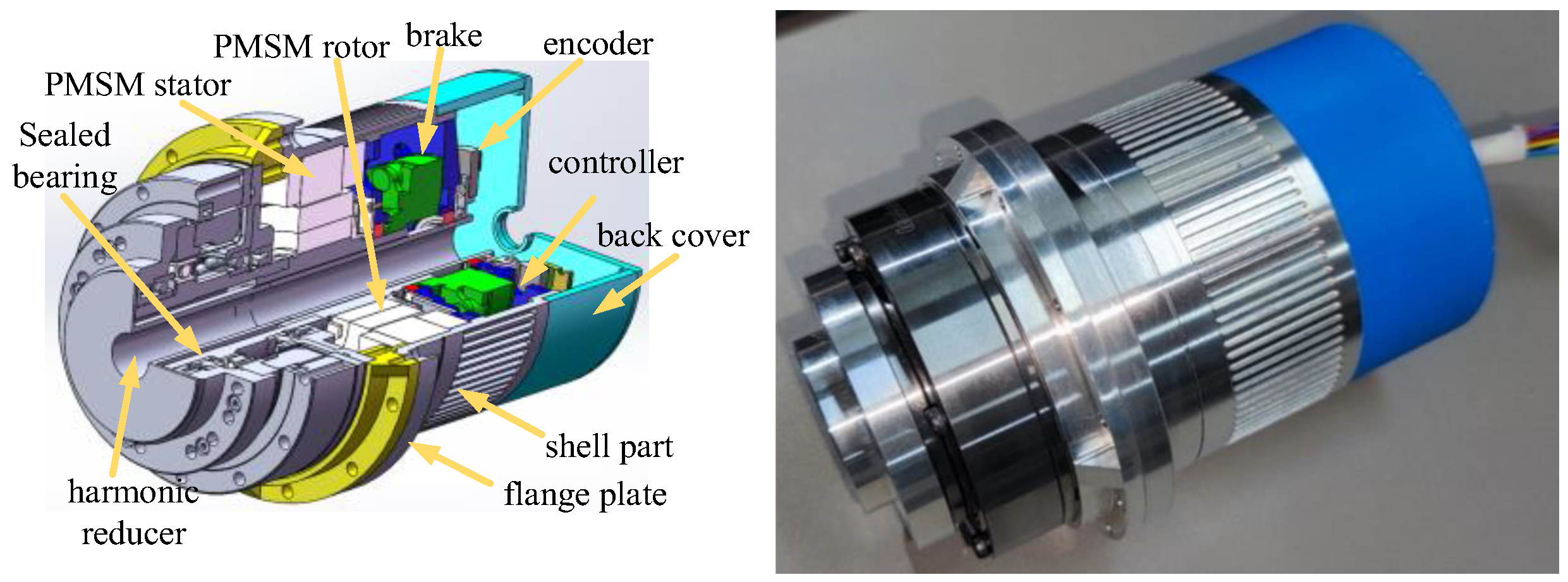
An integrated electromechanical actuator mainly comprises a motor, a reducer, a driver, a controller, and a position sensor. Actuators are mainly used in aviation, aerospace, robotics, guided weapons, medical devices, precision instruments, and other fields [1,2,3,4,5]. Reducers used in EMAs mainly include the parallel shaft gear reducer, planetary gear reducer, harmonic reducer, and rotary vector reducer. Harmonic reducers are commonly employed for actuators with high reduction ratios and medium power. The main factors that affect the transmission accuracy of harmonic reducers are clearance, friction, and stiffness. Spong et al. [6] proposed a dynamic modeling method for flexible joints. Based on the friction characteristics of harmonic reducers, Gandhi [7] associated friction with speed and position in the transmission system and used friction identification and nonlinear compensation methods to improve transmission accuracy. Taghirad et al. [8] established a dynamic model of a harmonic reducer, modeled friction losses at high and low speeds, and studied the characteristics of the model through simulation analysis. In the literature [9,10,11,12], the influence of temperature and load on friction has been deeply studied. Maré J. C. [9] proposed a generic framework for introducing load and temperature effects in the system-level friction model. Studies [10,11,12] have analyzed the effects of temperature and load on the friction torque of the harmonic reducer.

High-performance permanent magnet synchronous motors (PMSMs) are used in EMAs. Commonly employed in the control process of PMSM are PID control and state feedback control methods. However, PID control has the drawbacks of slow response speed and weak disturbance rejection. Advanced intelligent algorithms have been incorporated into PID controllers to improve PID control effects, such as genetic algorithm PID, self-tuning PID, artificial intelligence algorithm, and neural network PID [13,14,15,16]. Intelligent control algorithms have complex algorithms, high computational complexity, and pose challenges in engineering applications. Active disturbance rejection control (ADRC) operates independently of precise mathematical modeling of the controlled object. Contrary to traditional methods, it accounts for uncertain and complex factors, including unmodeled system components, external disturbances, nonlinear factors, and time-varying elements, by classifying these as the “total disturbance” of the system. ADRC utilizes a constructed extended state observer to estimate this “total disturbance” online and employs a control law for compensation [17]. Applications of ADRC in motor control have shown varying degrees of improvement in motor control efficacy [18,19,20]. Jin et al. [21] implemented a novel type of linear ADRC, replacing the PID controller, to effectively control a hydraulic cylinder servo system, acknowledging the characteristics of high-order coupling in the electrohydraulic system. Hu et al. [22] established an ADRC control method based on LuGre friction compensation to study the effect of nonlinear friction on the transmission accuracy of the photoelectric stabilization platform. Sira-Ramírez et al. [23] employed ADRC based on high gain generalized proportional integral observers for PMSM large disturbance trajectory tracking systems. Li et al. [24] used second-order ADRC to improve the disturbance rejection and transmission accuracy in the PMSM position control process. Research has been conducted on built-in PMSM control by using ADRC for position sensorless control [25].

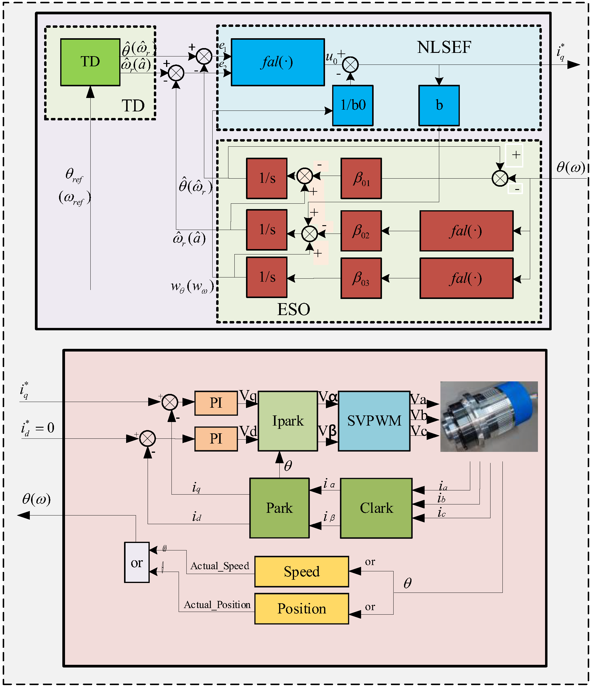
To mitigate the impact of nonlinear friction on the precision of EMA transmission, this study proposes an improved ADRC method based on the magnetic field-oriented control (FOC) method. The EMA friction model was added to the IADRC through feedforward compensation to improve the transmission accuracy. First, a mathematical model of the PMSM is presented. Based on this model, combined with the ADRC control principle, an EMA speed loop/position loop composite second-order ADRC is constructed. In the nonlinear error feedback link, a fuzzy control algorithm is incorporated to achieve the adaptive functionality of the EMA control algorithm. The relationship between the no-load friction torque and torque current is derived based on the transmission model of a harmonic reducer. The friction model was established through experimental methods and added to the ADRC control model through feedforward compensation. Based on the above research, an EMA drive control system was developed using STM32F4 as the main control chip, and the aforementioned control strategies were experimentally verified. The experimental results were evaluated and analyzed using the integral of time absolute error (ITAE) and the root mean square error (RMSE).

2. Mathematical Model of the PMSM Established Using the FOC Method

The PMSM is frequently utilized as a torque source in high-performance EMA applications. The PMSM mathematical model mainly includes the voltage equation, magnetic linkage equation, torque equation, and mechanical equation. To simplify the analysis without affecting the control, the winding current is assumed to be a symmetrical three-phase sinusoidal current, motor core saturation is ignored, and the eddy current and hysteresis losses of the motor are not considered. The PMSM adopts the FOC method, which offers the advantages of fast dynamic response, smooth torque, and stable low-speed control. By using FOC, the voltage equation in the d-q coordinate system is

$$\left\{\begin{array}{l}{u}_d=R_s{i}_d+\frac{d{\psi }_d}{dt}-\omega {\psi }_q\\ u_q=R_s{i}_q+\frac{d{\psi }_q}{dt}+\omega {\psi }_d\end{array}\right.$$

(1)

The d-q axis magnetic linkage equation is

$$\left\{\begin{array}{l}{\psi }_d=L_d{i}_d+{\psi }_f\\ {\psi }_q=L_q{i}_q\end{array}\right.$$

(2)

The electromagnetic torque equation is

$$T_e=1.5p_n[{\psi }_f{i}_q+(L_d-L_q)i_d{i}_q]$$

(3)

The second Newton law applied to the motor rotor is

$$J\frac{d{\omega }_r}{dt}=T_e-T_L-B{\omega }_r$$

(4)

In Equations (1)–(4), Rs is the phase resistance, i_d and i_q are the d-axis and q-axis currents, u_d and u_q are the d-axis and q-axis voltages, L_d and L_q are the d-axis and q-axis inductances, ψ_d and ψ_q are, respectively, the d-axis and q-axis magnetic linkages, p_n is the number of pole pairs, T_e is the electromagnetic torque, J is the rotational inertia, T_L is the load torque, B is the damping coefficient, ψ_f is the permanent magnet magnetic flux, ω is to the electrical angular velocity, and ω_r is the mechanical angular velocity.

$$\omega =p_n{\omega }_r$$

(5)

For surface-mounted PMSM, L_d = L_q. When i_d = 0 or L_d = L_q, Equation (3) can be simplified as

$$T_e=1.5p_n{\psi }_f{i}_q$$

(6)

3. Transmission Model of the Harmonic Reducer

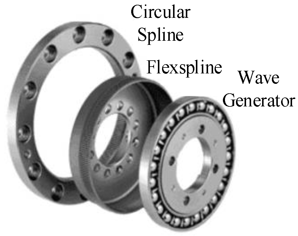
The harmonic reducer comprises a circular spine, a flexspline, and a wave generator, as shown in Figure 1. In the EMA, the circular spine is fixed and connects the rotor to the wave generator, whereas the flexspline is connected to the load end. During EMA operation, the wave generator acts as an active component; when the wave generator rotates, the flexspline generates controllable elastic deformation to transmit power. Approximately 30% of the teeth of the flexspline’s outer ring and the circular spline’s inner ring are in mesh, providing benefits such as a high transmission ratio and substantial load-bearing capacity.

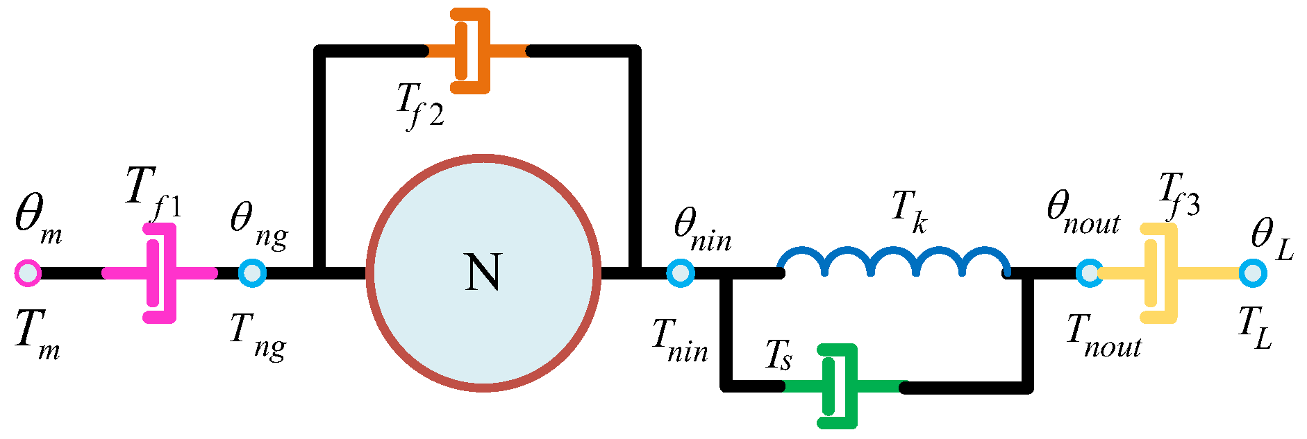
During the operation of the harmonic reducer, friction arises between the tooth surfaces of the flexspline and the circular spine, between the balls of the flexible bearing and the inner and outer rings, and between the wave generator and the contact surface of the flexspline. When the EMA reciprocates motion, the friction torque affects the transmission accuracy of the system. Friction disturbances in harmonic reducers cannot be ignored in high-performance control processes. High-precision control situations rely on friction compensation. Considering the flexspline as a torsion spring structure; considering the friction between the wave generator, flexspline, and circular spine; and considering the friction between the flexspline and the load, we established a nonlinear friction transmission model of the harmonic reducer based on the friction links in the transmission process, as shown in Figure 2.

In Figure 2, T_f1 is the friction generated by the wave generator, T_f2 refers to the friction between the flexspline and the circular spine, T_f3 refers to the friction generated by the flexspline, θ_m and T_m are, respectively, the rotor position and torque, θ_ng and T_ng are, respectively, the output positions and moments of the wave generator, θ_nin and T_nin are, respectively, the input angle and input torque of the flexspline torsion spring model, θ_nout and T_nout are, respectively, the displacement and output torque of the flexspline, Tk and Ts are, respectively, the torsion spring force and damping force of the flexspline torsion spring model, T_L is the output torque of the flexspline, and θ_L is the position of the flexspline.

The equilibrium equation of angular displacement and frictional torque between the wave generator and the flexspline is

$$\left\{\begin{array}{l}{T}_m=T_{ng}+T_{f1}\\ {\theta }_m={\theta }_{ng}\end{array}\right.$$

(7)

The equilibrium equation for the angular displacement and friction moment between the flexspline and the circular spine is

$$\left\{\begin{array}{l}{T}_{ng}=\frac{1}{N}{T}_{nin}+T_{f2}\\ {\theta }_{ng}=N{\theta }_{nin}\end{array}\right.\left\{\begin{array}{l}{T}_k=K_L\ast \Delta \theta \\ T_{nin}=T_k+T_s\\ T_{nin}=T_{nout}\end{array}\right.$$

(8)

The friction torque T_f acting on the harmonic reducer is T_f = T_f1 + T_f2 + T_f3. The friction torque T_f3 acting on the load end under low speeds and heavy loads is much smaller than the friction torque T_f1 acting on the motor and wave generator end under high speeds and light loads and can be ignored; that is, T_f3 ≈ 0. T_L = T_nout = T_k + T_s, and T_nout = f(Δθ, K_L). f(Δθ, K_L) = T_k + T_s = T_L. k is the stiffness coefficient of the harmonic drive. Thus, the relationship between the input torque, friction torque, and output torque of the harmonic reducer can be expressed as follows:

$$\left\{\begin{array}{l}{T}_L=f(\Delta \theta ,K_L)\\ T_m=\frac{f(\Delta \theta ,K_L)}{N}+T_f(t,B,{\omega }_r,\dots )\\ \Delta \theta =\frac{{\theta }_m}{N}-{\theta }_L\\ f(\Delta \theta ,K_L)=K_L(\frac{{\theta }_m}{N}-{\theta }_L)\end{array}\right.$$

(9)

where K_L is the equivalent stiffness coefficient of the harmonic reducer, neglecting the rotational inertia of the reducer, J is the rotational inertia of the motor rotor, J_L is the rotational inertia of the load end, and f(Δθ, K_L) = T_L. The relationship between the motor torque Te and the wave generator torque T_m is

$$\left\{\begin{array}{l}{T}_e=J\frac{d^2{\theta }_m}{d{t}^2}+T_m\\ \\ T_L=J_L\frac{d^2{\theta }_L}{d{t}^2}=f(\theta ,K_L)\end{array}\right.$$

(10)

The nonlinear friction torque obtained from Equations (9) can be expressed as

$$T_f(t,B,{\omega }_r,\dots )=T_m-\frac{T_L}{N}$$

(11)

Here, it is assumed that the load is purely inertial. The nonlinear friction force T_f of the harmonic reducer can be expressed as

$$\begin{array}{l}{T}_f(t,B,{\omega }_r,\dots )=T_m-\frac{1}{N}{T}_L\\ =1.5p_n{\psi }_f{i}_q-J\frac{d^2{\theta }_m}{d{t}^2}-\frac{1}{N}{J}_L\frac{d^2{\theta }_L}{d{t}^2}\end{array}$$

(12)

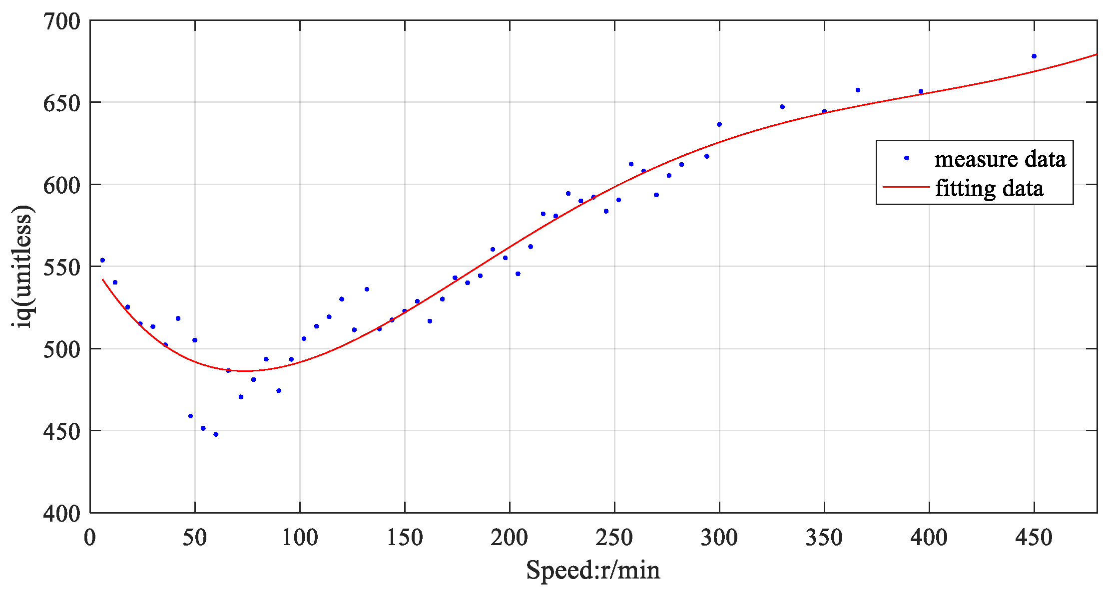
When unloaded and running at a constant speed, Equation (12) can be simplified as

$$T_f(t,B,{\omega }_r,\dots )=1.5p_n{\psi }_f{i}_q$$

(13)

As can be seen from Equation (13), the friction torque is related to the torque current i_q. During no-load and constant speed operation, the change rule of friction torque can be obtained by measuring the torque current i_q at different speeds and fitting the i_q change curve.

4. Improved ADRC Control Principle

4.1. Composite Second-Order ADRC Control Principle

ADRC does not rely on the precise mathematical model of the controlled object and can perform real-time estimation and compensation for internal and external disturbances in the system [27].

ADRC mainly includes a tracking differentiator (TD), an extended state observer (ESO), and nonlinear state error feedback (NLSEF). The TD executes rapid, non-overshoot tracking of target signals. The ESO monitors the system output and both internal and external disturbances. It isolates interference signals from the controlled output and incorporates compensation for these signals into the control law, thereby enhancing the system’s disturbance rejection capabilities [28,29,30]. NLSEF combines the output of TD and the state variable observation estimation output of ESO in a nonlinear manner and then acts on the controlled object after combining it with the “total disturbance” estimation of the system by ESO. The second-order ADRC principle is illustrated in Figure 3.

The TD discrete expression is

$$\left\{\begin{array}{l}{x}_1(k+1)=x_1(k)+T{x}_2(k)\\ x_2(k+1)=x_2(k)+Tfhan(x_1(k)-x_{in}(k),x_2(k),r,h_1)\end{array}\right.$$

(14)

The TD ensures that x₁ converges to the input signal x_in, x₂ is the derivative of the input signal, r is the speed factor and determines the tracking speed, T is the sampling time, and h₁ is the filtering factor. fhan(·) is the fastest synthesis function, represented as

$$fhan(\cdot )=\left\{\begin{array}{l}d=r{h}_1;\hspace{1em}\hspace{1em}{d}_0=h_{1}d\\ y=x_1+h_1{x}_2-x_{in}(k);\hspace{1em}{a}_0=\sqrt{d^2+8r\left|y\right|}\\ a=\left\{\begin{array}{l}{x}_2+\frac{(a_0-d)}{2},\left|y\right|>d_0\\ x_2+\frac{y}{h_1},\left|y\right|\le d_0\end{array}\right.\\ fst=\left\{\begin{array}{l}-\frac{ra}{d},\left|a\right|\le d\\ -rsign(a),\left|a\right|>d\end{array}\right.\end{array}\right.$$

(15)

The ESO discrete expression is

$$\left\{\begin{array}{l}e(k)=z_1(k)-y(k)\\ z_1(k+1)=z_1(k)+T(z_2(k)-{\beta }_{01}e(k))\\ z_2(k+1)=z_2(k)+T(z_3(k)-{\beta }_{02}fal(e(k),{\alpha }_{01},\delta )+bu(k))\\ z_3(k+1)=z_3(k)-T{\beta }_{03}fal(e(k),{\alpha }_{02},\delta )\end{array}\right.$$

(16)

where e(k) is the error signal, y(k) is the system output, z₁(k) is the tracking signal of y(k), z₂(k) is the tracking signal of z₁(k), z₃(k) is the total disturbance of the system, z₃(k) is feed back to the control variable u(k) for compensation, and b is the compensation factor. β₀₁, β₀₂, and β₀₃ are the output error correction gains, α₀₁ and α₀₂ are the nonlinear factors, and δ is the filtering factor.

The NLSEF discrete expression is

$$\left\{\begin{array}{l}{e}_1(k)=x_1(k)-z_1(k)\\ e_2(k)=x_2(k)-z_2(k)\\ u_0(k)={\beta }_{1}fal(e_1(k),{\alpha }_1,\delta )+{\beta }_{2}fal(e_2(k),{\alpha }_2,\delta )\\ u(k)=u_0(k)-\frac{z_3(k)}{b_0}\end{array}\right.$$

(17)

where e₁(k) and e₂(k) are error signals, and β₁ and β₂ are, respectively, the error gain and differential gain. When 0 < α < 1, fal(·) achieves a mathematical fitting of “small error with large gain, large error with a small gain.” Fuzzy control, variable gain PID, and intelligent control are based on the control concept of “small error with a large gain, large error with small gain” to adjust the output. fal(·) is a nonlinear feedback function and can be expressed as follows:

$$fal(\cdot )=\left\{\begin{array}{l}{\left|e\right|}^{\alpha }\mathrm{sgn}(e),\left|e\right|>\delta \\ \frac{e}{{\delta }^{(1-\alpha )}},\left|e\right|\le \delta \end{array}\right.$$

(18)

In the EMA control process, a commonly employed strategy is the cascade PI three-loop control, where the current loop constitutes the innermost loop, the speed loop serves as the middle loop, and the position loop functions as the outermost loop. The composite second-order ADRC combines the original speed loop and position loop PI(D) controllers into a single ADRC controller, thus improving the system response speed and reducing overshoot. The principle of the PMSM composite second-order ADRC structure established using the FOC method is shown in Figure 4. w_θ is the total disturbance in position mode, and w_ω is the total disturbance in velocity mode. θ is the measured angle of the rotor, and ω is the speed of the rotor.

In the composite second-order ADRC control mode, the control structure of the speed loop is the same as that of the position loop, except for the different input variables of the controller and the control parameters of the ADRC. By adjusting the input of TD and the control parameters of ADRC, speed-mode and position-mode operation can be achieved. The parameters that must be adjusted in second-order ADRC mainly include r and h in TD; β₀₁, β₀₂, and β₀₃ in ESO; and β₁ and β₂ in NLSEF. Although there are many parameters that must be adjusted, the three stages have their own engineering significance, and the principle of separate directional adjustment can be used to adjust the parameters of each stage.

4.2. Fuzzy ADRC Control Principle

During the operation of the EMA, the load is variable, and long-term service may cause changes in lubrication conditions and contact surface wear, resulting in parameter drift in the Stribeck friction model. In addition, parameters such as inductance, resistance, and magnetic linkage may drift with temperature changes. To adapt to the time-varying characteristics of the model, the control parameters of the controller must be modified adaptively.

However, ADRC does not possess parameter self-correction capability. To impart adaptive capability to ADRC, fuzzy logic control is integrated. Online adjustment of ADRC parameters is facilitated through the application of fuzzy rules. The fuzzy ADRC control method can adjust control parameters online according to different working states and obtain the most suitable control parameters within the set parameter variation range. Fuzzy control is integrated into the ADRC controller, and the control parameters of ADRC are adaptively adjusted based on the deviation and deviation rate of change.

NLSEF is added to the error integration link Equation (19), and the fuzzy control method is used to achieve self-tuning of the NLSEF parameters in ADRC. Fuzzy rules are used for fuzzy inference based on the input deviation e₁ and the change rate e₂ of the deviation to achieve online adjustment of the NLSEF coefficients and achieve adaptive ability:

$$\left\{\begin{array}{l}{e}_1(k)=z_{11}(k)-z_{21}(k)\\ e_2(k)=z_{12}(k)-z_{22}(k)\\ e_0={\displaystyle \int e_{1}dt}\\ u_0(k)={\beta }_{0}fal(e_0(k),{\alpha }_0,\delta )+{\beta }_{1}fal(e_1(k),{\alpha }_1,\delta )+{\beta }_{2}fal(e_2(k),{\alpha }_2,\delta )\\ u(k)=u_0(k)-\frac{z_{23}(k)}{b_0}\end{array}\right.$$

(19)

The inputs of fuzzy controllers in fuzzy ADRC are e₁ and e₂, and the outputs are Δβ₀, Δβ₁, and Δβ₂. In fuzzy PID control, based on the variation of e₁ and e₂, fuzzy subsets of five language variables, namely {“Negative Big (NB),” “Negative Small (NS),” “Zero (ZO),” “Positive Small (PS),” and “Positive Big (PB)”} are often used, or fuzzy subsets of seven language variables, namely {“Negative Big (NB),” “Negative Medium (NM),” “Negative Small (NS),” “Zero (ZO),” “Positive Small (PS),” “Positive Medium (PM),” and “Positive Big (PB)”} are often used. The control accuracy of seven fuzzy subsets is better than that of five fuzzy subsets. Here, β₀, β₁, and β₂ have the same control effect as k_i, k_p, and k_d, so seven subsets are selected here. Common membership functions include triangle membership, Z/S membership, trapezoid membership, and Gaussian membership, and in order to reduce the workload of operations, triangular membership functions are used for each fuzzy variable. The established fuzzy rules are presented in

Table 1. Δβ₀, Δβ₁, and Δβ₂ fuzzy rules.

e1	e2
	NB	NM	NS	ZO	PS	PM	PB
NB	NB/PB/PS	NB/PB/NS	NM/PM/NB	NM/PM/NB	NS/PS/NB	ZO/ZO/NM	ZO/ZO/PS
NM	NB/PB/PS	NB/PB/NS	NM/PM/NB	NS/PS/NM	NS/PS/NM	ZO/ZO/NS	ZO/NS/ZO
NS	NB/PM/ZO	NM/PM/NS	NS/PM/NM	NS/PS/NM	ZO/ZO/NS	PS/NS/NS	PS/NS/ZO
ZO	NM/PM/ZO	NM/PM/NS	NS/PS/NS	ZO/ZO/NS	PS/NS/NS	PM/NM/NS	PM/NM/ZO
PS	NM/PS/ZO	NS/PS/ZO	ZO/ZO/ZO	PS/NS/ZO	PS/NS/ZO	PM/NM/ZO	PB/NM/ZO
PM	ZO/PS/PB	ZO/ZO/NS	PS/NS/PS	PS/NM/PS	PM/NM/PS	PB/NM/PS	PB/NB/PB
PB	ZO/ZO/PB	ZO/ZO/PM	PS/NM/PM	PM/NM/PM	PM/NM/PS	PB/NB/PS	PB/NB/PB

.

The variation surfaces of β₀, β₁, and β₂ obtained from the domain of each variable and fuzzy reasoning are shown in Figure 5.

The modified parameters Δβ₀, Δβ₁, and Δβ₂ are obtained using the fuzzy rule table and the deblurring algorithm. The control parameters in NLSEF are obtained after correction by using Equation (20). Thus, ADRC parameter self-tuning is realized, and the adaptive ability of the system can be improved by adjusting and controlling the control parameters in NLSEF in real time. β₀₀, β₁₀, and β₂₀ are the initial values; select the initial value according to the empirical method:

$$\left\{\begin{array}{l}{\beta }_0={\beta }_{00}+\Delta {\beta }_0\\ {\beta }_1={\beta }_{10}+\Delta {\beta }_1\\ {\beta }_2={\beta }_{20}+\Delta {\beta }_2\end{array}\right.$$

(20)

The structural diagram of fuzzy ADRC is shown in Figure 6.

5. EMA Control System Design

The three-dimensional cross-sectional and physical views of the EMA developed with an integrated hollow shaft harmonic reducer are depicted in Figure 7. The incremental encoder disk is fixed on the hollow shaft of the spindle by using an adhesive that has high aging resistance, impact resistance, and shear strength. To ensure the reliability of bonding, the viscosity is 750–1750 cps, and the shear strength is greater than 19 MPa. The main parameters of the harmonic reducer in

Table 2. Parameters of the harmonic reducer.

Reduction Ratio	Transmission Direct Efficiency at Rated Load	Max Torque (N.m)	Max Input Speed (rev/min)	Theoretical Lifespan (h)	Weight (kg)
100	0.69	49	7000	15,000	0.8

. The main parameters of the PMSM in

Table 3. PMSM parameters.

Resistance (Ω)	Inductance (mH)	Rated Torque (N.m)	Peak Torque (N.m)	Max Speed (rev/min)	Peak Current (A)	Inertia
100	0.65	0.72	3.8	3100	27	3.04 ∗ 10−5 kgm

.

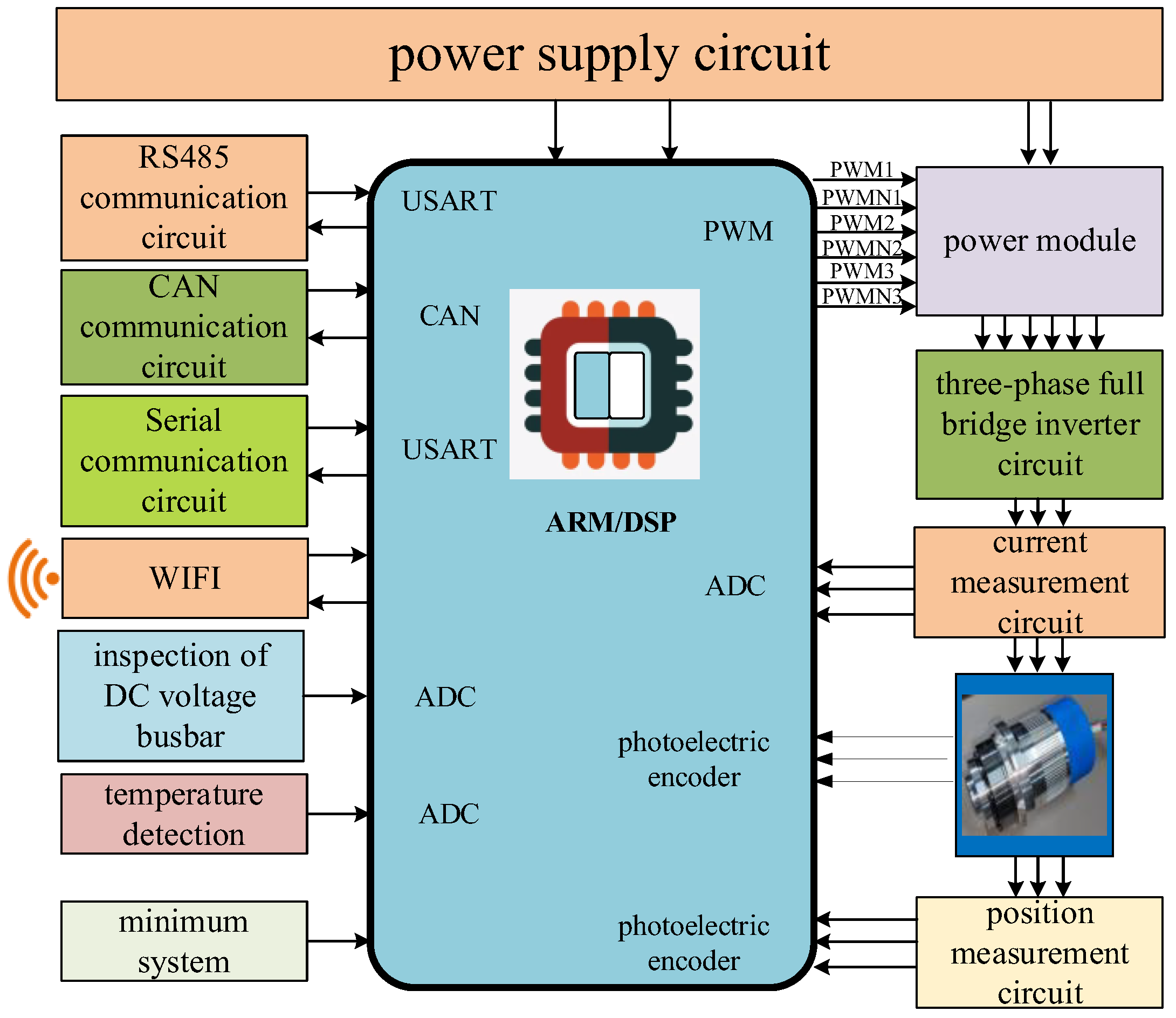
For the proposed IADRC control algorithm, STM32F4 is used as the main control chip for verification. The controller possesses abundant built-in resources, supports floating-point operations, and encompasses various communication interfaces, including two advanced timers, TIM1 and TIM8, dedicated to motor control. Functions such as position detection, current detection, USART, CAN, and RS485 can be performed using this chip. The hardware circuit structure of the EMA is illustrated in Figure 8.

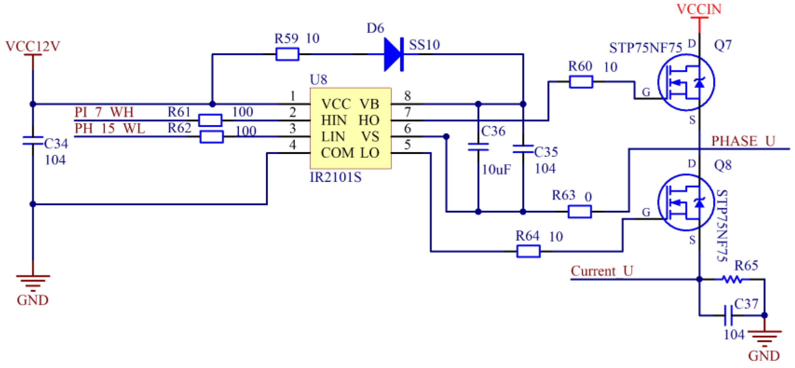
The N-type IRFS3607 MOSFET is used as the power device in the inverter circuit, and IR2101S is used as the power driver chip. The driving circuits for the V and W phases in a three-phase system are consistent. Using the U-phase as an example, the inverter circuit is briefly explained. The U-phase drive circuit for three-phase current is illustrated in Figure 9.

The IO ports corresponding to advanced timer 1 and advanced timer 8 in STM32F4 can output six complementary and symmetrical PWM waves. The working voltage of the IR2101S power driver chip is 12V, and IR2101S receives PWM signals from the MCU to drive IRFS3607. IRFS3607 is an N-type MOSFET.

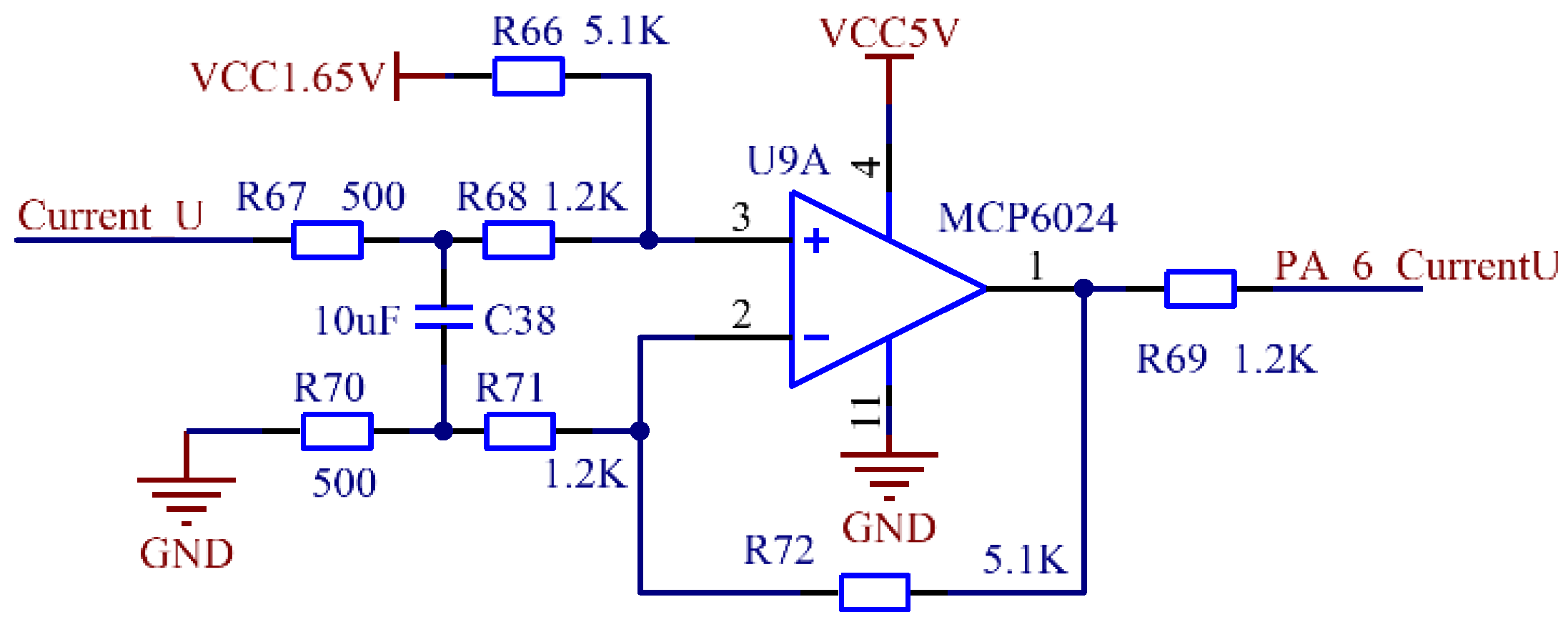
Rotor position data constitutes crucial information in the FOC process. Current resistance sampling methods encompass single, double, and triple resistance sampling. The single resistance sampling method, while structurally simple, complicates software processing. Conversely, double resistance sampling may induce three-phase asymmetry. Triple resistance sampling requires an operational amplifier, which is costly; however, it offers the advantages of accurate sampling and relatively simple program processing. For the convenience of software processing, the triple resistance sampling method is adopted in the control system. The U, V, and W three-phase control circuits are the same. Here, the U-phase is taken as an example; the U-phase sampling circuit is shown in Figure 10.

MCP6024 has a large magnification. According to the virtual shorting of the amplifier, there is no current flowing through both ends of the operational amplifier. The current flowing through R2 and R7 is equal, and the current flowing through R10 and R14 is equal:

$$\frac{V_{+}-V_{cc}}{R_2}=\frac{V_{in}-V_{+}}{R_6+R_7},\frac{V_{out}-V_{-}}{R_{14}}=\frac{V_{-}}{R_9+R_{10}}$$

(21)

Let a = R6 + R7 = R9 + R10 and b = R2 = R14, Substituting these into Equation (21), we obtain

$$\frac{V_{+}-V_{cc}}{b}=\frac{V_{in}-V_{+}}{a},\frac{V_{out}-V_{-}}{b}=\frac{V_{-}}{a}$$

(22)

Solving Equation (22) yields

$$V_{+}=\frac{b{V}_{in}+a{V}_{cc}}{a+b},V_{-}=\frac{a{V}_{out}}{a+b}$$

(23)

Under virtual shorting, V+ = V−, Can be obtained

$$V_{out}=\frac{b}{a}{V}_i+V_{cc}=1.65+5.1V_{in}$$

(24)

As can be seen from Equation (24), the voltage at both ends of the sampling resistor is biased by 1.65 V and amplified by 5.1 times. The sampling resistor is selected as a high-precision resistor of 10 m Ω and 2 W, with a theoretical maximum sampling current of 14.14 A. If the maximum amplitude of the sinusoidal current of the motor is 10 A, the voltage range input to the amplifier end is −0.1–0.1 V. According to Equation (24), the output voltage of the amplifier is calculated as 1.14–2.16 V, which can be directly inputted into the ADC sampling pin of the motor, providing a large safety margin.

6. Experimental Analysis

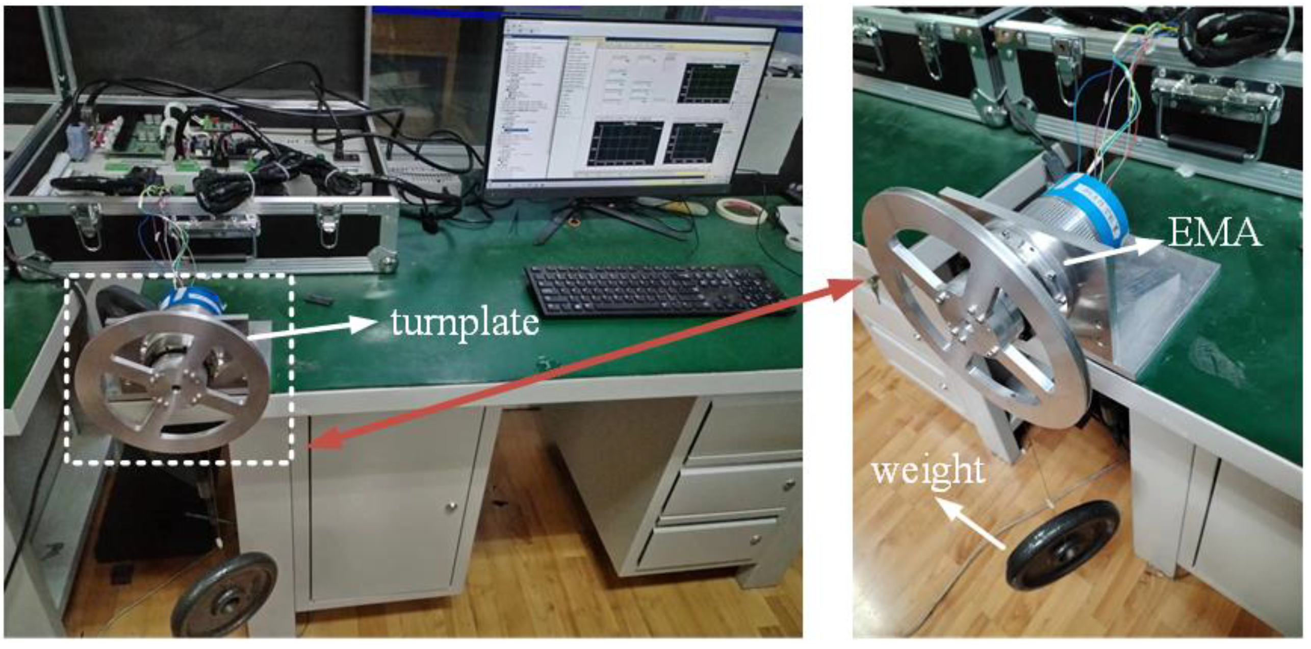
According to Equation (13), friction torque can be determined by measuring the torque current i_q at a constant speed without load. This article performed experimental analysis on frictional forces in the counter-clockwise rotation direction. The inertia of the reducer was disregarded, and it was assumed that the torque during no-load operation equals the friction torque during uniform motion. A friction model was developed by measuring torque values at various speeds and fitting the data. This model was incorporated into the control system through feedforward compensation, effectively eliminating friction disturbances. Friction torque testing was performed on the RT-Cube platform, which is capable of achieving a minimum control cycle for the motor within 100 µs. Moreover, this platform allows for the online modification of any control parameter and the online monitoring of any system variable during the control process. The tests were made at a room temperature of approximately 25 °C and a relative humidity ranging from 40% to 70%RH. The experimental platform and the test results obtained using the Gaussian fitting method are shown in Figure 11 and Figure 12, respectively.

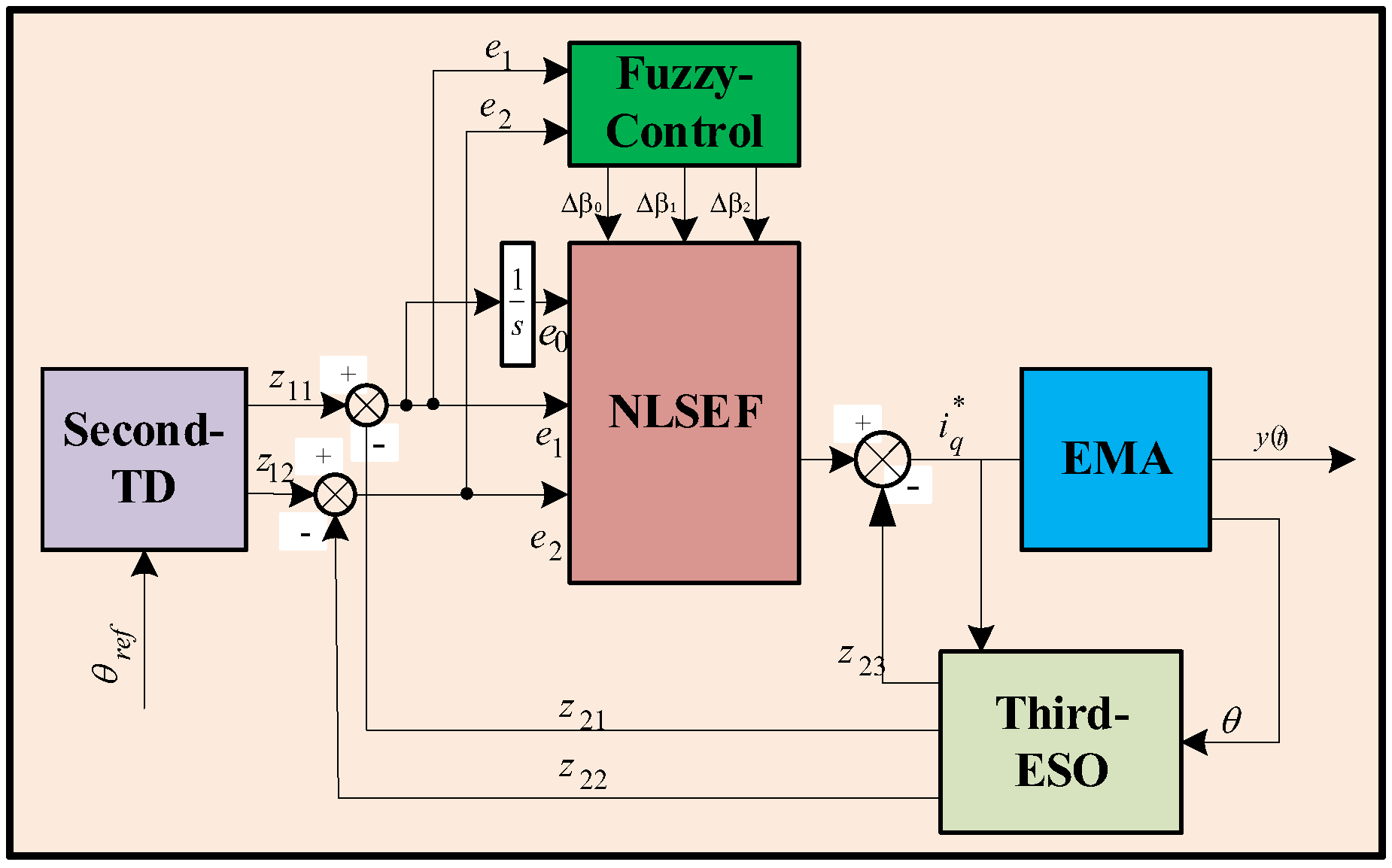
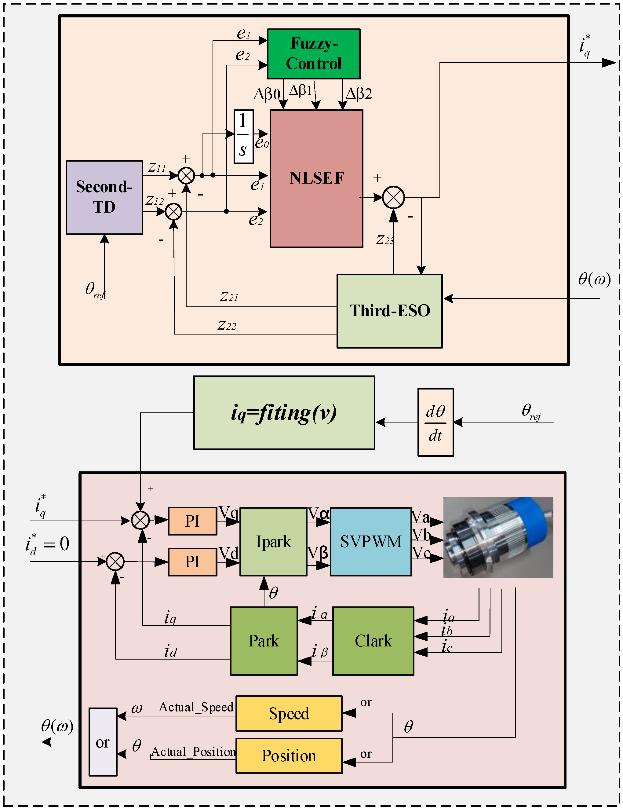
According to the fitting equation, the friction force at different speeds was obtained. The friction force, corresponding to the torque current, was compensated for and attenuated by adjusting the torque current at various speeds. The IADRC controller was constructed by integrating the frictional torque current into the second-order fuzzy ADRC control model through feedforward compensation, as shown in Figure 13.

In the EMA speed mode, the current loop of all three control methods adopts PI control mode, and the speed loop adopts PI, ADRC, and IADRC, respectively. An IADRC controller with a step speed of 6 rev/min was used. The control parameters for the three controllers were empirically set. The main parameters to be adjusted in the TD are the r and h₁. The r affects the tracking effect. A larger r corresponds to a shorter transition time and thus a faster tracking response. However, very large r leads to overshoot and oscillation. When the r is constant and the h₁ is large, the tracking signal error is large; when the h₁ is small, the noise suppression is more prominent. However, when the h₁ is too small, the ability of the TD to suppress noise will be weakened. The disturbance compensation factor b₀ mainly affects the disturbance compensation capacity. If the system disturbance is significant, b₀ should be slightly larger; if the system disturbance is small, b₀ should be marginally lower. Directional adjustment is adopted. 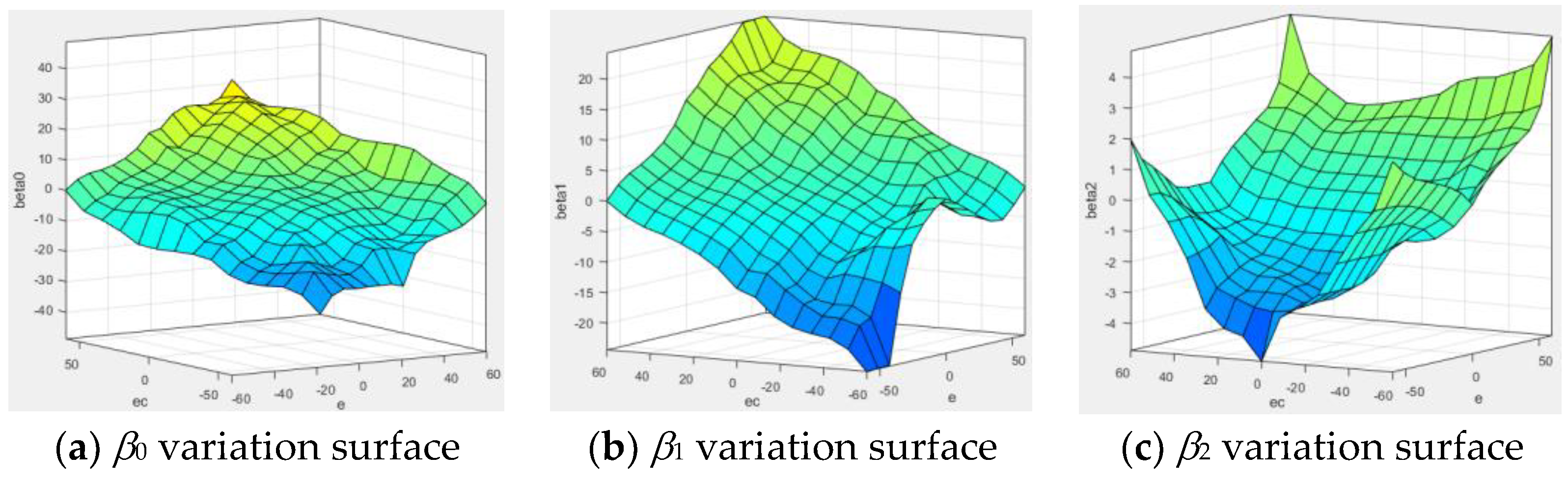When we set α₀₁ = α₀₂ = 1, fal(e,α,δ) can be linearized to fal(e,α,δ) = e. The values for the parameters β₀₁, β_02, and β₀₃ need to be adjusted in practical applications according to the system output. The tuning rules for these parameters are listed in

Table 4. Tuning rules for β₀₁, β_02, and β₀₃.

Constant Parameters	System Response Phenomena	Tuning Rules
β02, β03	Oscillation occurs	Decrease β01
	Divergence occurs	Decrease β01
	Steady-state high-frequency oscillation occurs	Increase β01
β01, β03	High-frequency oscillation occurs	Decrease β02
	Disturbance rejection performance decrease	Increase β02
	Oscillation amplitude increase	Increase β02
β01, β02	Overshoot occurs	Increase β02
	Response time is long	Increase β03
	Large oscillation occurs	Decrease β03

. Notably, when one parameter is tuned, the other two remain constant.

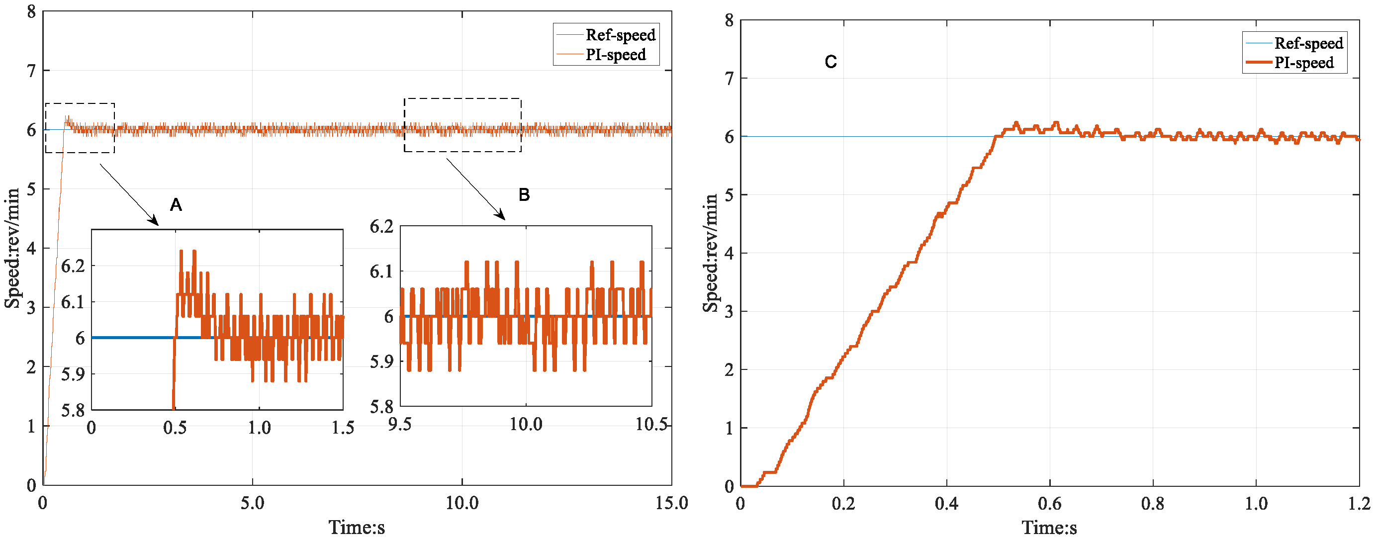
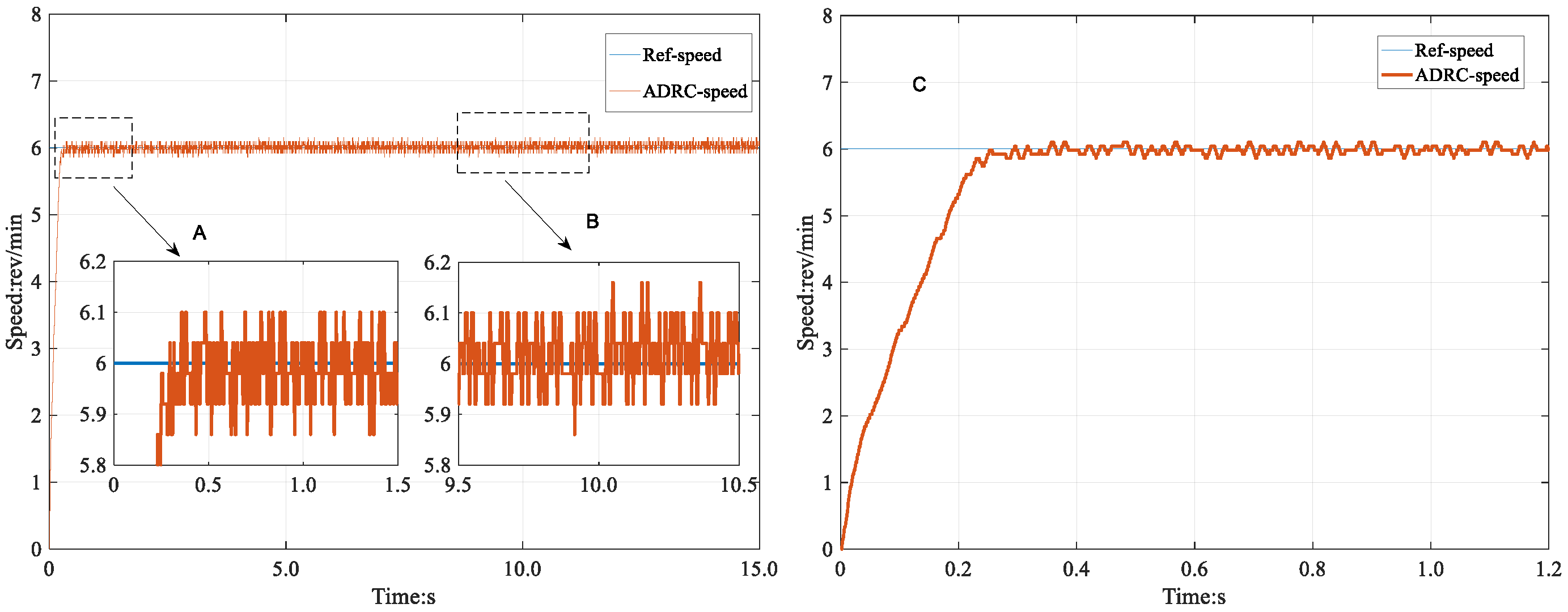
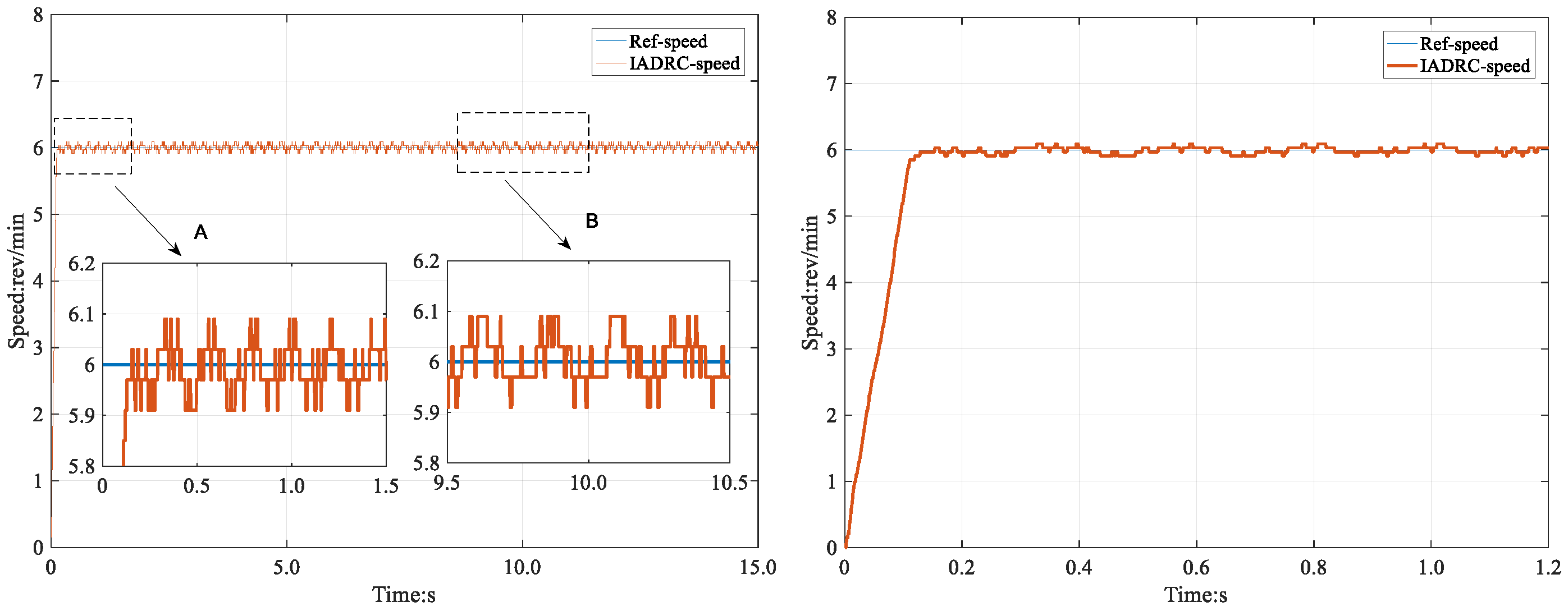
The results obtained using PI control method and the enlarged image of the step response are shown in Figure 14. The results obtained using ADRC control method and the enlarged image of the step response are shown in Figure 15. The results obtained using IADRC control method and the enlarged image of the step response are shown in Figure 16. As can be seen in the locally enlarged image A, the PI control method, ADRC control method, and feedforward compensation fuzzy IADRC reached a steady state in 0.65, 0.25, and 0.20 s, respectively. The PI control method experienced an overshoot before reaching the steady state, with a maximum speed of 6.2 rev/min and an overshoot of 3.33%. The other two control methods quickly achieved the target speed without overshooting. The steady-state speed error of all three control methods was 0.1 rev/min. By comparing the locally enlarged image B of ADRC and IADRC, it can be concluded that the IADRC control method has a lower speed oscillation frequency in the steady state.

Common performance indicators of the control system include integrated square error (ISE), integrated time square error (ITSE), integrated absolute error (IAE), and integrated time absolute error (ITAE). Different performance indicators have different priorities.

The ITAE criterion can better reflect the system’s response speed, oscillation characteristics, and steady-state errors, and has good selectivity for different controllers:

$$ITAE={\displaystyle {\int }_0^{\infty }t\left|e(t)\right|dt}$$

(25)

The ITAE calculation results for the three control methods within 0–1s are presented in

Table 5. ITAE calculation results of three methods.

Control Mode	PI	ADRC	IADRC
ITAE	47.714 (rev/min)*s2	11.559 (rev/min)*s2	5.727 (rev/min)*s2

.

The unit of ITAE is “(rev/min)*s²”. The ITAE calculation result within 0–1 s of IADRC was 15.445 (rev/min)*s², thus indicating the optimal control performance of IADRC. The number of encoder lines is 2880, and after fourfold frequency, it is 11,520. The position input signal is y = 115,200*sin(0.05*pi*t), and the unit of y is the carving line number of the encoder (LNE). The main parameters in the experimental are shown in

Table 6. Main parameters in the experiment.

Name	Parameter Value
Encoder	2880 PPR
Reduction ratio	50
Counter weight	25 N
Disc radius	0.1 m
Load	2.5 N·m

.

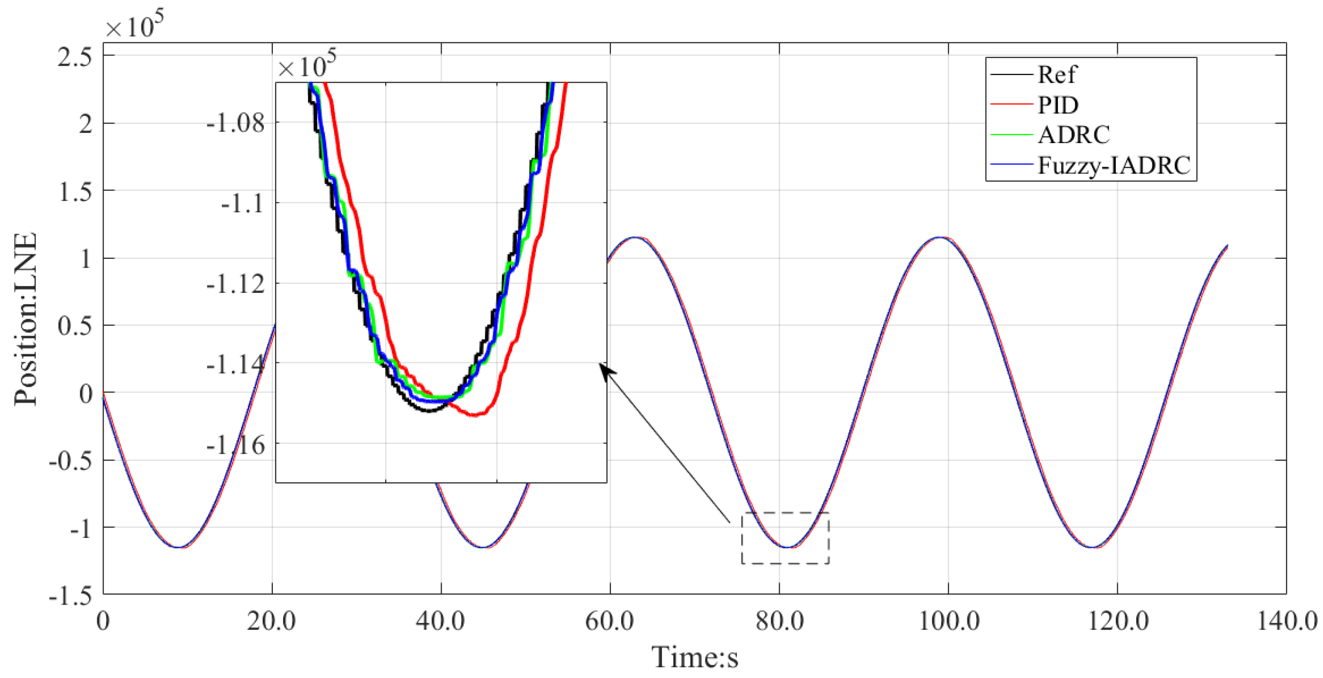
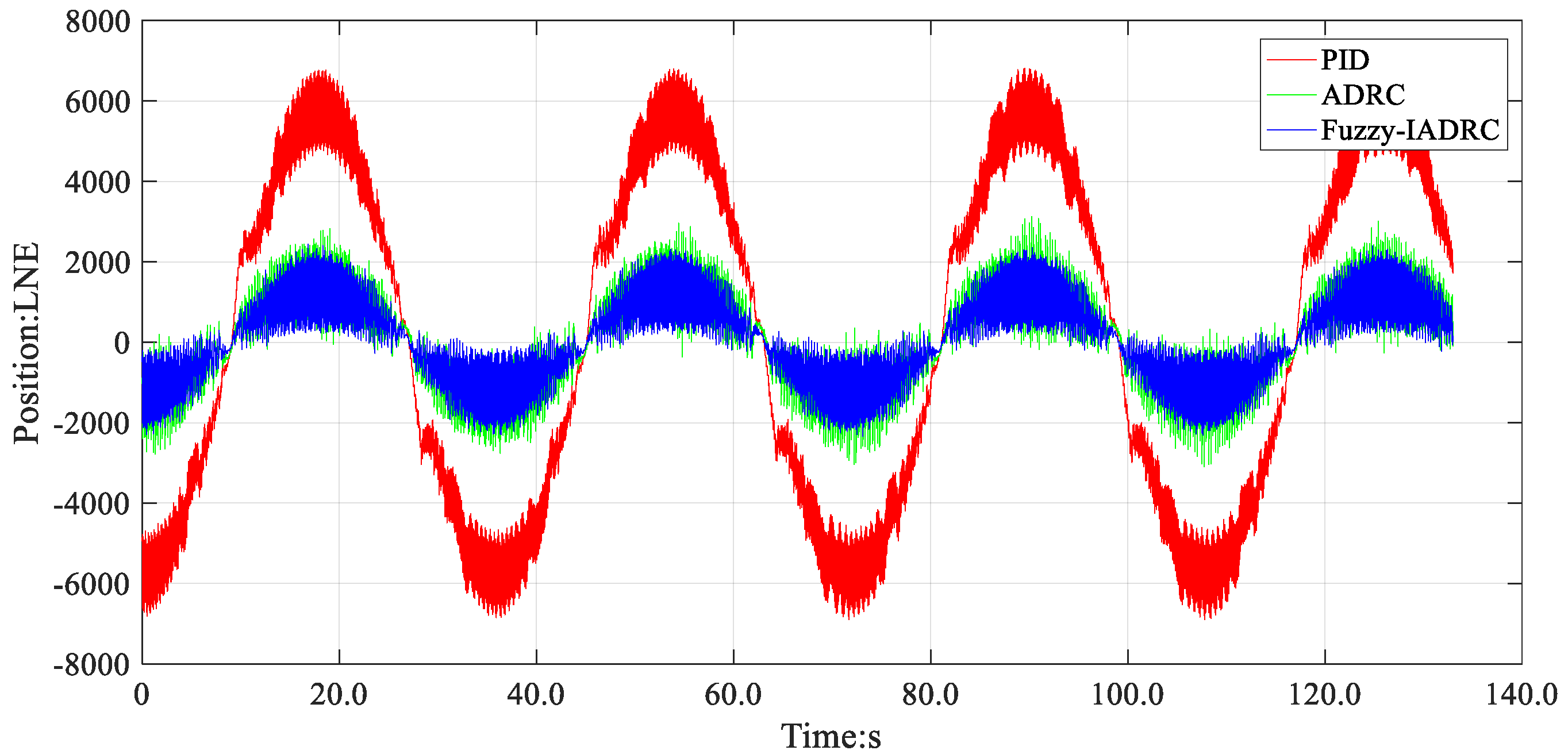
In the EMA position mode, three control configurations were implemented: PID (position loop) + PI (speed loop) + PI (current loop); ADRC (position loop) + PI (current loop); and IADRC (position loop) + PI (current loop). Data were recorded after the system stabilized. The position tracking results under no-load conditions for the three control methods are illustrated in Figure 17. The corresponding position tracking error results are presented in Figure 18.

The RMSE and peak-to-peak calculation results of tracking error are presented in

Table 7. No−load test results.

Control Mode	RMSE	Peak-to-Peak Values
PID	4165.1	13685 LNE
ADRC	1201.4	6218 LNE
IADRC	1040.8	4780 LNE

.

As can be seen from Figure 18 and Table 7, the ADRC control method yielded higher accuracy than the PID control when under load. After adding friction feedforward compensation, the RMSE and peak-to-peak values of position error improved. The peak-to-peak value of IADRC was 1438 less than that of ADRC. The RMSE of IADRC reduced by approximately 160.6 compared with ADRC.

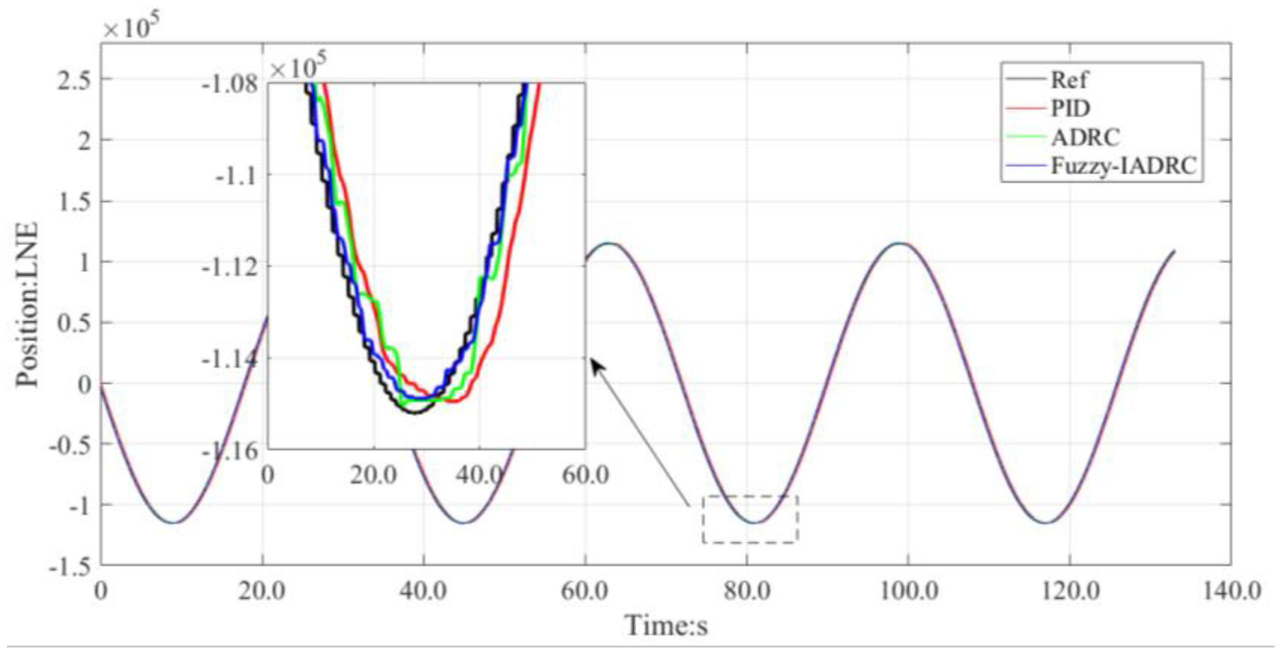
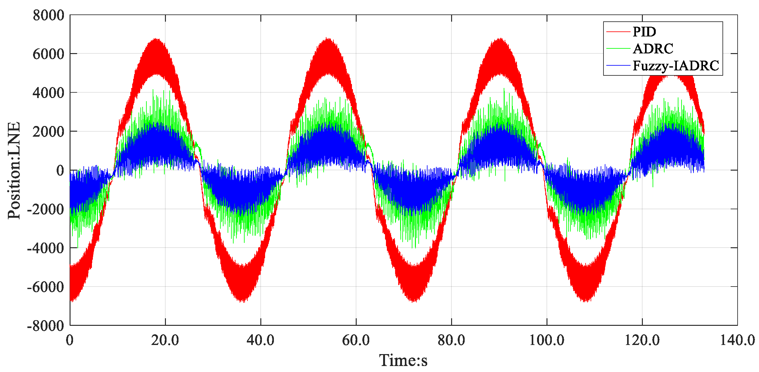
Record data after the system stabilizes. In the position-mode test under 2.5 Nm load conditions, the position tracking results for the three control methods are depicted in Figure 19. Correspondingly, the position tracking error results for the three control methods are illustrated in Figure 20. It is noteworthy that this load (2.5 Nm) represents 6.25% of the rated torque.

The RMSE and peak-to-peak calculation results of PID, ADRC, and friction feedforward compensation fuzzy IADRC control methods under load are presented in

Table 8. Load test results.

Control Mode	RMSE	Peak-to-Peak Values
PID	4183.6	13,773 LNE
ADRC	1636.4	8242 LNE
IADRC	1046.8	4869 LNE

.

As can be seen from Figure 20 and Table 8, the ADRC control method yielded higher accuracy than the PID control when under load. After the addition of friction feedforward compensation, the root mean square and peak-to-peak values of position error improved. The peak-to-peak value of IADRC was 3373 less than that of ADRC. The RMSE of IADRC was reduced by approximately 410.4 compared to ADRC.

7. Conclusions

Aiming at the problem of EMA control accuracy, this paper adopts high-performance IADRC and friction feedforward compensation methods. The PMSM mathematical model was established, and a second-order composite ADRC control strategy was developed for the PMSM speed loop and position loop based on the FOC model. The ADRC controller demonstrates several superior characteristics not present in the PI controller. To address the issue of ADRC controller parameter adaptation, fuzzy control was integrated into the nonlinear state error feedback link, facilitating self-tuning of ADRC parameters. Furthermore, a model for EMA transmission was developed, and the relationship between friction torque and torque current i_q was analyzed. Furthermore, on the RT-Cube platform, the torque current i_q at different speeds was measured and then added to the current loop control through feedforward compensation, determining controller parameters through empirical methodologies. In addition, speed-mode and position-mode experiments were conducted in the PI control mode, ADRC control mode, and IADRC control mode. Moreover, the experimental results of the speed step response were analyzed using the IATAE criteria. The IADRC control mode yielded the smallest calculation result and the best control performance. Neglecting the inertia of the reducer, assuming that the no-load running torque is equal to the friction torque during uniform motion, the experimental results of sinusoidal position tracking were analyzed, and the results were evaluated using RMSE and peak-to-peak values. Under conditions of pure inertial load, the integration of friction feedforward compensation combined with the implementation of the IADRC control method enhances the accuracy of EMA transmission.

References

1. Zhang, Y.; Zhao, C.; Dai, B.; Li, Z. Dynamic simulation of permanent magnet synchronous motor (PMSM) electric vehicle based on Simulink. Energies 2022, 15, 1134. [Google Scholar] [CrossRef]
2. Zhou, D.; Luo, K.; Shen, Z.; Zou, J. Vector-Space-Decomposition-Based Power Flow Control of Single-Stage-Multiport-Inverter-Fed PMSM Drive for Hybrid Electric Vehicles. IEEE Trans. Ind. Electron. 2023, 1–11. [Google Scholar] [CrossRef]
3. Chuyen, T.D.; Van Hoa, R.; Co, H.D.; Huong, T.T.; Ha, P.T.T.; Linh, B.T.H.; Nguyen, T.L. Improving control quality of PMSM drive systems based on adaptive fuzzy sliding control method. Int. J. Power Electron. Drive Syst. 2022, 13, 835–845. [Google Scholar] [CrossRef]
4. Assoun, I.; Idkha, L.; Nahid-Mobarakeh, B.; Meibody-Tabar, F.; Monmasson, E.; Pacault, N. Wide-Speed Range Sensorless Control of Five-Phase PMSM Drive under Healthy and Open Phase Fault Conditions for Aerospace Applications. Energies 2022, 16, 279. [Google Scholar] [CrossRef]
5. Li, P.; Xu, X.; Yang, S.; Jiang, X. Open circuit fault diagnosis strategy of PMSM drive system based on grey prediction theory for industrial robot. Energy Rep. 2023, 9, 313–320. [Google Scholar] [CrossRef]
6. Spong, M.; Khorasani, K.; Kokotovic, P. An integral manifold approach to the feedback control of flexible joint robots. IEEE J. Robot. Autom. 1987, 3, 291–300. [Google Scholar] [CrossRef]
7. Gandhi, P.S.; Ghorbel, F.H.; Dabney, J. (Eds.) Modeling, Identification, and Compensation of Friction in Harmonic Drives. In Proceedings of the 41st IEEE Conference on Decision and Control, Las Vegas, NV, USA, 10–13 December 2002; pp. 160–166. [Google Scholar]
8. Taghirad, H.D.; Belanger, P.R. Modeling and parameter identification of harmonic drive systems. ASME J. Dyn. Syst. Meas. Control 1998, 120, 439–444. [Google Scholar] [CrossRef]
9. Maré, J.C. Friction modelling and simulation at system level: Considerations to load and temperature effects. Proc. Inst. Mech. Eng. Part I J. Syst. Control. Eng. 2015, 229, 27–48. [Google Scholar] [CrossRef]
10. Martineau, J.P.; Chedmail, P. Caractérisation Expérimentale et Modélisation du Comportement des Réducteurs Harmonic Drive. In Proceedings of the Congrès Mondial des Engrenages et des Transmissions de Puissance, Paris, France, 16–17 March 1999; pp. 1089–1100. [Google Scholar]
11. Martineau J, P. Modelisation Experimentale des Reducteurs Harmonic Drive, Application a la Determination des Parametres Minimaux d’un Robot Souple Trois Axes[D]. Ph.D. Thesis, Nantes University, Nantes, France, 1996. [Google Scholar]
12. Marc, M.J.C.B. Conception Préliminaire des Actionneurs Électromagnétiques Basée sur les Modèles: Lois d’estimations et Règles de Conception pour la Transmission de Puissance Mécanique; INSA: Toulouse, France, 2012. [Google Scholar]
13. Yadav, D.; Verma, A. Comperative performance analysis of PMSM drive using MPSO and ACO techniques. Int. J. Power Electron. Drive Syst. 2018, 9, 1510–1522. [Google Scholar] [CrossRef]
14. Salem, W.A.A.; Osman, G.F.; Arfa, S.H. (Eds.) Adaptive Neuro-Fuzzy Inference System Based Field Oriented Control of PMSM & Speed Estimation. In Proceedings of the 2018 Twentieth International Middle East Power Systems Conference (MEPCON), Cairo, Egypt, 18–20 December 2018; pp. 626–631. [Google Scholar]
15. Liu, Z.; Wei, H.; Zhong, Q.-C.; Liu, K.; Xiao, X.-S.; Wu, L.-H. Parameter estimation for VSI-fed PMSM based on a dynamic PSO with learning strategies. IEEE Trans. Power Electron. 2016, 32, 3154–3165. [Google Scholar] [CrossRef]
16. Barkat, S.; Tlemçani, A.; Nouri, H. Noninteracting adaptive control of PMSM using interval type-2 fuzzy logic systems. IEEE Trans. Fuzzy Syst. 2011, 19, 925–936. [Google Scholar] [CrossRef]
17. Han, J. From PID to active disturbance rejection control. IEEE Trans. Ind. Electron. 2009, 56, 900–906. [Google Scholar] [CrossRef]
18. Gao, S.; Wei, Y.; Zhang, D.; Qi, H.; Wei, Y. A modified model predictive torque control with parameters robustness improvement for PMSM of electric vehicles. Actuators 2021, 10, 132. [Google Scholar] [CrossRef]
19. Wang, X.; Zhu, H. Active disturbance rejection control of bearingless permanent magnet synchronous motor based on genetic algorithm and neural network parameters dynamic adjustment method. Electronics 2023, 12, 1455. [Google Scholar] [CrossRef]
20. Bao, H.; He, D.; Zhang, B.; Zhong, Q.; Hong, H.; Yang, H. Research on dynamic performance of independent metering valves controlling concrete-placing booms based on fuzzy-LADRC controller. Actuators 2023, 12, 139. [Google Scholar] [CrossRef]
21. Jin, K.; Song, J.; Li, Y.; Zhang, Z.; Zhou, H.; Chang, X. Linear active disturbance rejection control for the electro-hydraulic position servo system. Sci. Prog. 2021, 104, 00368504211000907. [Google Scholar] [CrossRef]
22. Hu, X.; Han, S.; Liu, Y.; Wang, H. Two-axis optoelectronic stabilized platform based on active disturbance rejection controller with LuGre friction model. Electronics 2023, 12, 1261. [Google Scholar] [CrossRef]
23. Sira-Ramírez, H.; Linares-Flores, J.; García-Rodríguez, C.; Contreras-Ordaz, M.A. On the control of the permanent magnet synchronous motor: An active disturbance rejection control approach. IEEE Trans. Control. Syst. Technol. 2014, 22, 2056–2063. [Google Scholar] [CrossRef]
24. Li, S.; Li, J. Output predictor-based active disturbance rejection control for a wind energy conversion system with PMSG. IEEE Access 2017, 5, 5205–5214. [Google Scholar] [CrossRef]
25. Du, B.; Wu, S.; Han, S.; Cui, S. Application of linear active disturbance rejection controller for sensorless control of internal permanent-magnet synchronous motor. IEEE Trans. Ind. Electron. 2016, 63, 3019–3027. [Google Scholar] [CrossRef]
26. Lu, Y.S.; Hwang, C.S. Tracking Control of a Harmonic Drive Actuator with Sliding-Mode Disturbance Observers. In Proceedings of the 2009 IEEE/ASME International Conference on Advanced Intelligent Mechatronics, Singapore, 14–17 July 2009; pp. 1798–1803. [Google Scholar]
27. Huang, Y.; Xue, W. Active disturbance rejection control: Methodology and theoretical analysis. ISA Trans. 2014, 53, 963–976. [Google Scholar] [CrossRef] [PubMed]
28. Jingqing, H. Active Disturbance Rejection Control Technique—The Technique for Estimating and Compensating the Uncertainties. Master’s Thesis, National Defense Industry Press, Beijing, China, 2008. [Google Scholar]
29. Wang, Y.; Fang, S.; Hu, J. Active disturbance rejection control based on deep reinforcement learning of PMSM for more electric aircraft. IEEE Trans. Power Electron. 2022, 38, 406–416. [Google Scholar] [CrossRef]
30. Rong, Z.; Huang, Q. A new PMSM speed modulation system with sliding mode based on active-disturbance-rejection control. J. Cent. South Univ. 2016, 23, 1406–1415. [Google Scholar] [CrossRef]
Figure 1. Structure of the harmonic reducer [26].
Actuators 12 00445 g001
Figure 2. Harmonic drive friction model.
Actuators 12 00445 g002
Figure 3. Block diagram of second-order ADRC control.
Actuators 12 00445 g003
Figure 4. Block diagram of composite second−order ADRC.
Actuators 12 00445 g004
Figure 5. β0, β1, and β2 variation surfaces.
Actuators 12 00445 g005
Figure 6. Fuzzy ADRC control block diagram.
Actuators 12 00445 g006
Figure 7. Structure diagram and photograph of the EMA.
Actuators 12 00445 g007
Figure 8. Hardware circuit structure of the EMA.
Actuators 12 00445 g008
Figure 9. U-phase drive circuit.
Actuators 12 00445 g009
Figure 10. U-phase current sampling circuit.
Actuators 12 00445 g010
Figure 11. EMA friction torque test bench.
Actuators 12 00445 g011
Figure 12. EMA friction moment fitting experiment.
Actuators 12 00445 g012
Figure 13. IADRC control block diagram.
Actuators 12 00445 g013
Figure 14. PI test results of no-load step signal.
Actuators 12 00445 g014
Figure 15. ADRC test results of no-load step signal.
Actuators 12 00445 g015
Figure 16. IADRC test results of no-load step signal.
Actuators 12 00445 g016
Figure 17. No−Load position tracking results.
Actuators 12 00445 g017
Figure 18. No−Load position error tracking results.
Actuators 12 00445 g018
Figure 19. Load position tracking results.
Actuators 12 00445 g019
Figure 20. Load position error tracking results.
Actuators 12 00445 g020