Abstract
It is difficult to achieve a high-precision motion control in hydraulic manipulators due to their structural redundancy, strong coupling of closed-chain structures, and flow–pressure coupling. In this paper, a high-precision motion control method for hydraulic manipulators is proposed based on the traditional virtual decomposition control (VDC). The method proposed avoids an excessive virtual decomposition of the hydraulic manipulator and requires fewer model parameters than the traditional VDC. Further, the control precision improved by combining an adaptive real-time update of the inertial parameters. Compared with MBC, the proposed control method improved the motion accuracy of the hydraulic manipulator by more than 40% and 20% under elliptical and triangular trajectories. The simulation results showed that the proposed control method reduced the maximum position errors in Cartesian space by 90.4%, 86.8%, 23.6%, and 44.3% compared with PID and model-based control (MBC) in the absence of disturbances. The maximum position error in Cartesian space was reduced by 76.5% compared with that of MBC in a simulation with external disturbances. It can be seen from all the simulation results that with the proposed control method, the position error of the manipulator was less than 50 mm. The proposed control method effectively improved the motion precision of the examined hydraulic manipulator.
1. Introduction
Hydraulic manipulators are widely used in construction [1], rescue [2,3], port hoisting [4], deep-sea exploration [5], and other heavy-load operations due to their characteristics of high power, large load carriage capacity, stable transmission, etc. However, they are structurally redundant, present heavy coupling of closed-chain structures, and flow–pressure coupling. These problems make it difficult to achieve high-precision motion in hydraulic manipulators compared with electrically driven manipulators. Therefore, it is of great theoretical and practical significance to research the high-precision control of hydraulic manipulators.
At present, the available hydraulic manipulator motion control methods are the model-free control and the model-based control. The model-free control includes PID control [6], neural network control [7], fuzzy control [8,9], and so on. Lee [10] proposed an adaptive PID control with the advantages of the adaptive time-delay control. Li [11] researched the cooperative motion control of multiple manipulators based on distributed recurrent neural networks. Mohammad [12] introduced a new novel discrete adaptive fuzzy controller for manipulators that are powered by electricity, which addresses the system’s nonlinearity and uncertainty. The model-free control avoids the establishment of complex dynamic models of manipulators and is widely used in electric-drive manipulators. However, it cannot avoid the influence of inertial force, non-linearity of the hydraulic drive, and closed-chain coupling on the control precision of hydraulic manipulators, which limits the improvement of control precision.
Therefore, the model-based control is more suitable for the high-precision control of hydraulic manipulators. Traditional model-based control methods are the model predictive control [13], the sliding mode control [14], the adaptive control [15], and so on. The traditional model-based control requires the establishment of complete dynamic models of hydraulic systems and manipulators. The mainstream dynamic modeling methods of hydraulic manipulators include the Lagrange method [16], the Kane method [17], and the Newton–Euler method [18]. Jouko Kalmari [19] proposed a nonlinear model predictive control based on numerical optimization in which a particular objective function is minimized to improve motion precision. Ding [20] proposed a model-based control method (MBC) for high-precision trajectory tracking control in manipulators based on the Lagrange method. It compensates for the nonlinear dynamic characteristics of both the manipulator and the hydraulic actuator. However, the dynamic model based on the Lagrange method will cause high dimensionality in multi-body manipulators, which reduces the computing efficiency. Zhou [21] created an adaptive robust controller combined with a backstepping approach based on the Kane method, which reduced the influence of external disturbance. Zhao [22] proposed a modal space sliding mode control based on the mathematical model built by the Newton–Euler method. However, control methods based on traditional modeling ignore the closed-chain structures in hydraulic manipulators. Therefore, it is impossible to accurately model the coupling problem generated by the closed-chain structures, which reduces the control precision.
To solve the problem of strong coupling caused by the closed-chain structures of hydraulic manipulators, Zhu [23,24] proposed VDC, which virtually decomposes the closed-chain structures into open-chain subsystems. Each subsystem is modeled and controlled separately. This control method was applied by Koivumäki [25,26] to a three-degree-of-freedom manipulator and by Petrovic [27] to a seven-degree-of-freedom manipulator to improve the control precision. However, the structure of the manipulators was relatively simple in these previous studies. The hydraulic manipulator studied in this paper had a luffing mechanism between every two adjacent links. The luffing mechanism was combined with the links and the hydraulic cylinder to form multiple closed-chain structures. Each closed-chain structure needs to be decoupled when using the traditional VDC, which may cause a huge increase in the number of decomposed subsystems. A virtual equivalent component is here proposed to reduce the number of closed chains caused by the luffing mechanism. Thus, the complex luffing mechanism became equivalent to a simple component through virtual transformation. Each three closed-chain structure became equivalent to a closed-chain structure consisting of a virtual equivalent component, the links, the hydraulic cylinder, which reduced the number of subsystems. The complexity of modeling and the computational cost of the simulation were further reduced. The load distribution coefficient and the change of inertia parameters were calculated as in [25], considering a manipulator system with equivalent components.
A high-precision control method for hydraulic manipulators is proposed in this paper. A 13 m three-degree-of-freedom hydraulic manipulator was the research object. A virtual decomposition model of the overall manipulator structure was established with fewer modules than those used by the traditional method, and the complex closed-chain structure was decomposed into open-chain subsystems. At the same time, an adaptive updated method of uncertain inertia parameters is proposed to compensate for the structural dynamic characteristics of the manipulator. Finally, a simulation was carried out on the Simulink virtual prototype model to verify the effectiveness of the proposed control method.
This paper is organized as follows. The decomposition and dynamics of the manipu lator are presented in Section 2. The subsystem of hydraulic actuators is introduced in Section 3. The adaptive design of the inertial parameters and the stability analysis of the system are described in Section 4 and Section 5, respectively. The simulation model of the whole manipulator system is established in Section 6, and different simulation conditions were designed to validate the proposed method. The contribution of this study and the future research plans are discussed in Section 7. Finally, Section 8 reports the conclusions of this study.
2. Materials and Methods
In this paper, a 13 m three-degree-of-freedom hydraulic manipulator was selected as the research object, as shown in Figure 1. Subfigure (a) is the real manipulator studied in this work. Subfigure (b) is the 3D model and hydraulic schematic and the red arrows mean coordinates at joints.
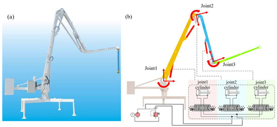
Figure 1.
The hydraulic manipulator system studied in this work. (a) the real manipulator studied in this work. (b) the 3D model and hydraulic schematic and the red arrows mean coordinates at joints.
The virtual decomposition process began with the joint decomposition and link division of the hydraulic manipulator’s structure, which established the basic model framework. Then, we calculated the kinematics/dynamics parameters of each subsystem based on each coordinate set up on the divided open-chain structure. The load distribution coefficient in each subsystem was calculated at the last. Through these steps, we could solve the internal force vector, and the whole dynamic model of the manipulator after virtual decomposition was established.
2.1. Joint Decomposition and Link Partitioning
The hydraulic manipulator in Figure 2a was first decomposed into subsystems using the virtual cutting points (VCPs). The VCPs oriented the virtual decomposition of the manipulator. The manipulator’s parts after virtual cutting still maintained their position and direction. Force and torque could be applied on one part to affect another part. Therefore, the VCPs can be considered as points of transmission of effects between two adjacent subsystems.
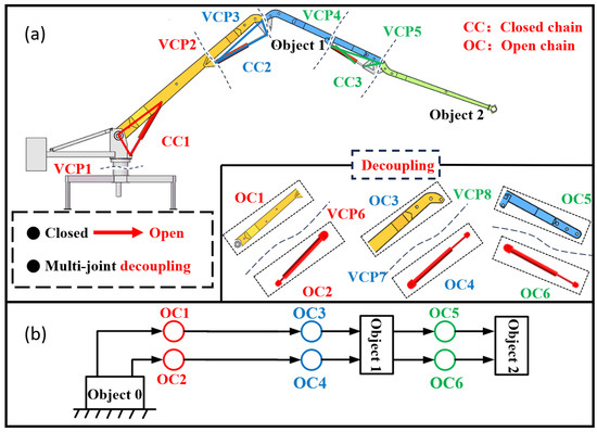
Figure 2.
Schematic diagram of the virtual decomposition control of the studied hydraulic manipulator. (a) the position of the virtual cutting point in the manipulator. (b) the simple oriented graph of the manipulator structure.
Figure 2a shows the decomposition process of the whole hydraulic manipulator system into multiple subsystems. The manipulator contained three closed-chain structures associated with the hydraulic cylinders. The directional diagram in Figure 3b illustrates the dynamic relationship between the substructures of the decomposed system. Each subsystem was defined as a node. A subsystem with only the initial node was defined as a source node, and a subsystem at the end of the structure was referred to as a sink node. Object 0 served as the source node, and object 2 served as the sink node.
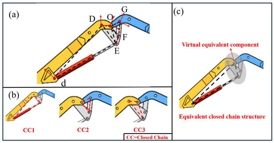
Figure 3.
Equivalent closed-chain structures in arm1 and arm2. (a) Multi closed chain structures consisted by luffing mechanism, hydraulic cylinder and links. The letters in the figure represent the coordinate systems at the hinge points, (b) Closed-chain structure, (c) Virtual equivalent component in the equivalent closed chain structure.
The closed-chain structure was decoupled using the traditional VDC to solve the structural coupling problem of hydraulic manipulators. A study [27] proposed a decomposition method to reduce the number of subsystems for its research object. However, the hydraulic manipulator we studied had a more complex structure with luffing mechanisms, as shown in Figure 3a. Figure 3a shows multi closed chain structures consisted by luffing mechanism, hydraulic cylinder and links. The letters in the figure represent the coordinate systems at the hinge points. If the closed-chain structure formed between the luffing mechanism, the links, and the hydraulic cylinder, shown in Figure 3b, was decomposed, the number of subsystems would increase, further increasing the difficulty of the modeling.
To solve this problem, a virtual equivalent component method is proposed in this paper.
The generalized coordinates of point D in the closed chain 1 in Figure 3b were transformed to obtain point O in the virtual equivalent component through the transformation matrix, according to Equation (1).
The position transformation matrix between point d and point D could be obtained using the same method:
Then:
Similarly, the matrix OUG of the coordinate frame G equivalent to O and the matrix EUF of the coordinate frame F equivalent to E was derived.
The complex luffing mechanisms became virtual equivalent components through the above processing. Three closed-chain structures were converted into one closed-chain structure and obtaining the structure “virtual equivalent component—links—hydraulic cylinder”, which reduced the number of subsystems.
The motion and force interactions between the subsystems were described by additional coordinate systems. Each closed-chain structure had five coordinate systems. Take 2(a) as an example: the coordinate systems {B1}, {B10}, {B11}, {B12}, and {T1} were set at the rotating joint and at the piston rod. The X direction of each coordinate system {B} pointed to the next coordinate system and formed a non-drive open chain. {T1} was the drive coordinate system of the hydraulic cylinder which constituted the drive open chain. These coordinate systems describe the motion and force interactions between subsystems, which are crucial for the system’s control.
2.2. Kinematic Analysis of the Closed Chains
The dynamics of the system was analyzed using the Newton—Euler method in Figure 4(1b,1c). Each closed chain was composed of four rigid bodies, including two connecting rods, two hydraulic cylinders three non-driven rotary joints, and one linear-driver joint.
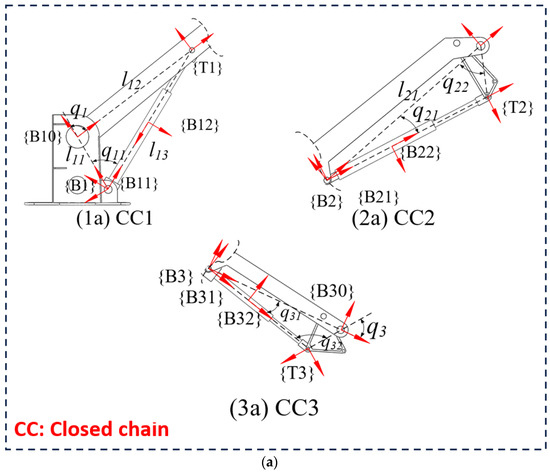
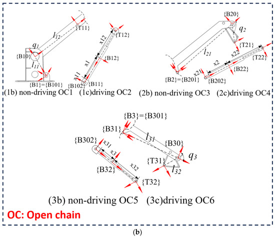
Figure 4.
(a) A closed chain. (b) Virtual decomposition of a closed chain to open chains.
In the Figure 4, 1a–3a are three hydraulic actuator assemblies of the hydraulic manipulator. 1b–3b and 1c–3c are open chains of 1a–3a that be virtual decomposed.
The relationship between the joint angles q1, q11, and q12, and the position of piston x1 is described as follows:
where l11 and l12 are the lengths of two adjacent links, x11 is the hydraulic cylinder barrel length, and x12 is the piston rod length.
The joint angular velocities 1, 11, 12 and velocity 1 can be obtained by Equations (7)–(9) as follows:
The combined linear/angular velocity vector expression in the link coordinate system A is as follows:
where and represent the linear velocity and the angular velocity vectors in the coordinate system A.
To calculate the motion chain of the system, we followed the path from the source node (object 0) to the sink node (object 3) along the directional graph. The linear/angular velocity vector of the link relative to the joint within a closed chain can be obtained using the recursive kinematics of the subsystem:
where OV = [0 0 0 0 0 0]T, zr = [0 0 0 0 0 1]T, and zf = [1 0 0 0 0 0]T. AUTB represents the transformation matrix of the force and moment vectors in the coordinate system B relative to the coordinate system A:
where represents the angle of deflection of the coordinate system B concerning A, rx, ry, rz represent the distance of the coordinate system B concerning A in the directions of x, y, and z.
Taking the transformation of the coordinate system B1 to B10 as an example, B1UB10, B1RB10, B1rB1B10× can be obtained:
Since the coordinate systems are located in the same plane, the Z direction is 0
To improve control precision, the concept of needed velocity was introduced in the VDC, which is different from the desired velocity of the reference trajectory relative to time. The needed velocity can be used for force/position control. Therefore, the desired velocity and the associated error, such as the force/position error, can be included in the needed velocity. Position control is achieved by incorporating position errors into the needed velocity. Therefore, the desired linear/angular velocity vector of the link relative to the joint is modified by Equation (14) as follows:
where the λ > 0 is the control gain.
2.3. Dynamics Analysis of the Closed Chains
According to [23], the complete dynamics analysis of a mechanical manipulator requires establishing dynamic equations for every virtual decomposed closed-chain structure. The first closed-chain structure was used as an example in this section.
Define A and B as coordinate systems fixed to the rigid body structure. Assume that the coordinate system A can be located at all points except for the center of mass. The coordinate system B is positioned at the mass center. The force vector and moment vector expression in the coordinate system A is as follows:
where the Afnet ∈ R3 and Amnet ∈ R3 represent the force vector and the moment vector in frame A.
The rigid body dynamics equation for a rigid body coordinate system can be derived by defining the net force/moment vector. The dynamic equation of a rigid body in free motion is expressed in the inertial system Io as:
where I3 ∈ R3×3 is the identity matrix, mA is the mass of the rigid body, Io ∈ R3×3 is the inertia matrix at the center of mass of the rigid body. vo ∈ R3 and wo ∈ R3 represent the linear velocity vector and the angular velocity vector at the center of mass, respectively. The net force/moment vectors applied to the mass center are denoted by the symbols fnet ∈ R3 and mnet ∈ R3.
This rigid body’s net force vector and moment vector in the coordinate system A can be expressed as:
The linear velocity, angular velocity, linear acceleration, and angular acceleration can be derived by considering Equation (15).
For a rigid body, the linear/angular velocity vector can be updated as
The linear acceleration/angular acceleration vector can be updated as
Combining Equation (22) and with Equation (19) and multiplying both sides of Equation (19) by , we can obtain the rigid body dynamics equation:
The closed-chain-driven force/moment vector TF ∈ R6 at a VCP can be obtained through the recursive dynamic calculation of the subsystem. It can be written as:
The force vector and moment vector T1F and T2F at the driving VCP of the open chains 1 and 2 can be expressed as:
where α1 and α2 are two load distribution coefficients, with α1 + α2 = 1, and is the internal force vector.
2.4. Calculation of Load Distribution Coefficients and Internal Force Vector
A previous study [25] provide a detailed calculation method of the internal force vector and load distribution coefficient.
The load distribution coefficient is an important parameter affecting the dynamic characteristics of hydraulic manipulators. The load distribution coefficients α1 and α2 describe the force distribution between two open-chain links in the x–y plane when Tf is applied to the closed-chain driver VCP.
Figure 5a shows the forces applied to the closed-chain driver VCP and the arbitrary force/moment vectorTf in the coordinate system {T}.
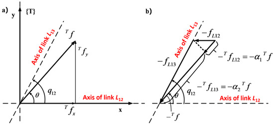
Figure 5.
Force analysis of the driving VCP in a closed chain. (a) The forces applied to the closed-chain driver VCP and the arbitrary force/moment vector Tf in the coordinate system. (b) The reaction forces −fL12 and −fL13.
The subsystem simultaneously applied a reaction force −Tf when the force vector Tf was applied from the driver VCP of the closed chain to its adjacent subsystem. The force vector −Tf produced the reaction forces −fL12 and −fL13. The reaction forces −fL12 and −fL13, as shown in Figure 5b, were decomposed into the force vectors −TfL12 and −TfL13 parallel to −Tf. The relationship can be expressed as follows:
Combining the law of sines and Equation (26), the expression of the load distribution coefficient sα1 and α2 can be derived as follows:
The calculation of the force/moment vector at the open-chain VCP required the calculation of the internal force vector Tη first. The calculation of the internal force vector Tη required to obtain the forces Tηfx along the x-axis and Tηfy along the y-axis and the moment Tηmz along the z-axis.
From Equation (16) we have:
Since friction in a hydraulic manipulator mainly exists between the hydraulic cylinder and the piston, the friction at the undriven joint is assumed to be 0. The following relationship can be derived from Equation (25):
By combining Equations (25) and (27)–(29), the expression of Tηfy can be derived as follows:
The desired net force vector and moment vector can be derived from the desired linear velocity vector and angular velocity vector:
Then, the force/moment vector required for the driving VCP of the open chains 1 and 2 can be written as:
In open chain 1, the force vector and moment vector are denoted by:
In open chain 2, the force vector and moment vector are denoted by:
The output force A required to close the hydraulic cylinder in the chain is:
3. Subsystem of the Hydraulic Actuator
In this section, the dynamics of the hydraulic actuator in the hydraulic manipulator was derived and calculated [23].
Let fc be the pressure and fu be the output force and define the ff as the friction force. So, we have:
According to Bernoulli’s flow equation, the pressure difference is proportional to the square variance of two flow rates via a valve port. Therefore, the flow gf is proportional to the product of the square root of the spool control signal and the pressure drop:
where k > 0 is a constant term, Δp > 0 indicates the pressure drop at the valve port, and u indicates the spool control signal.
The rates of the flow are defined as ga and gb as follows:
where cp1, cn1, cp2, cn2 are the valve port flow coefficients, Ps, Pr, Pa, and Pb are the system pressure, tank pressure, rod chamber pressure, and rod-less chamber pressure, respectively, v is a symbolic function.
The equations of pressure dynamics can be described in the following form:
where Sa and Sb represent the rod chamber area and the rod-less chamber area, respectively, c represents the piston rod displacement, and cm represents the stroke of the piston rod. Consider
Refer to the hydraulic cylinder flow continuity equation and Equation (38):
where fcr is the output force, and uf can be written as:
A physical quantity that reflects the flow capacity of the valve is the flow coefficient of the valve port. The flow capacity of the valve increases with the flow coefficient, and the pressure loss of the fluid via the valve port decreases. By using least squares identification, the flow coefficient’s value can be calculated.
The Equation of the regression matrix and identification terms is obtained by separating the flow coefficient contained in Equation (42) as follows:
Before the simulation, preparations were made to obtain chamber pressure, piston displacement, and other relevant parameters by arbitrarily designing a running trajectory. The following least squares technique was used to calculate the valve port flow coefficient and the effective elastic bulk modulus, to introduce the identified parameters into the control method.
The least squares method equation is written as:
The force term and the piston velocity term composed of the pressure feedback of two chambers were added to the control equation. The output force of the hydraulic cylinder and the speed of the piston were fed back to the control system in real time. The stability and control precision were controlled by the control valve-related output signal. The term ufd is determined according to the Equation (44)
with
ufd can be rewritten according to Equation (52) when the condition of Equation (51) is satisfied:
The vectors , and are updated as:
The γth elements of , , and are updated as:
4. Adaptive Design of the Inertial Parameters
The inertial parameters of a hydraulic manipulator are a group of time-varying parameters in the process of motion. The inertial parameters can be calculated and updated in real time to increase control precision. Based on Equation (32), the parameters to be estimated are separated linearly to obtain:
Taking closed chain 1 as an example, the net force vector and moment vector required for four rigid bodies are calculated as follows:
where KB1 ∈ R6×6, KB10 ∈ R6×6, KB11 ∈ R6×6, and KB12 ∈ R6×6 are the positive definite gain matrices B1 ∈ R13, B10 ∈ R13, B11 ∈ R13, and B12 ∈ R13. is an estimated parameter matrix containing mass, moment of inertia, product of inertia, and other parameters.
Select the function Φ as an updating law of 13 group parameters for each rigid body:
γ represents the γth parameter, and ρB1γ is the parameter updating gain. B1γ and B1γ are the upper and lower limits of B1γ, respectively.
SBi can be expressed as:
The equation for considering a time derivative is as follows:
5. Stability Analysis of the System
The VDC control law is designed according to the dynamics of the subsystems. The dependency vector x(t) of a subsystem is defined as a virtual function of L∞, and y(t) as a virtual function of L2. The L2-L∞ stability and convergence of the whole system can be guaranteed when each subsystem has the required stability and convergence. Define a scalar term corresponding to each VCP, called virtual power flow (VPF). VPF is the inner product of the velocity error and the force error and defines the dynamic interaction between subsystems. VPF plays a crucial role in the virtual stability of subsystems and ensures the L2-L∞ stability of the whole system.
Define a non-negative adjoint function and take its derivative as:
The dependency vector x(t) of the virtual decomposed subsystem is defined as the virtual function of L∞, and y(t) as a virtual function of L2, where 0 ≤ γs ≤ ∞, P and Q are two diagonally positive definite matrices, Φ and Ψ are coordinate systems placed at the driven cut point, PA and PC are VPFs. The inner product of the error of the force/moment vector and the error of the linear/angular velocity vector is known as PA:
The accessory vectors B1Vr − B1V and B10Vr − B10V of the first open chain are chosen as virtual functions of L2 and L∞. The non-negative adjoint function of the first open chain is:
where vB1 and vB10 are non-negative adjoint functions of the two links of the open chain 1:
The derivation of vB1 and vB10 in relation to time is obtained with:
The following equation is obtained by combining Equations (13), (16), (28), (30), (32) and (52):
The derivative of v1 in relation to time is:
In a similar manner, the time derivative of the second open chain non-negative adjoint function can be written as follows:
The simultaneity of Equations (24) and (33) can be obtained as follows:
Suppose a non-negative adjoint function is 0 and multiply by (TVr − TV)T:
The virtual stability of the first open chains and two zero mass objects can be proved. Now, let us address ()(fur – fu), which prevents the open chain’s stability.
Define a vector vc according to the hydraulic dynamics and control equations as follows:
It follows from Equations (44) and (47) that
The time derivative of vc satisfies the condition as follows:
Define B11Vr − B11V, B12Vr − B12V, and fcr − fc as virtual functions for both L2 and L∞. The second open chain’s non-negative adjoint function is redefined as follows:
and
The derivative of the Lyapunov function of the hydraulic manipulator is a negative definite function, while the energy function is positively definite. Equation (70) can be derived:
The virtual stability of the first and second open chains can be proved by the above Equations.
6. Simulation and Analysis
6.1. Simulation Platform
A complete hydraulic manipulator simulation platform was built by Matlab/Simulink to test the control precision of the proposed method.
The hydraulic system is shown in Figure 6. The V means the velocity of piston rod. The u means valve control voltage and the P is pressure in the two chambers of the hydraulic cylinder. The F means drive force. It was composed of the hydraulic power module, a valve-controlled cylinder module, and a liquid–solid interaction module. The hydraulic power module included a hydraulic pump and a hydraulic oil tank. The valve-controlled cylinder module consisted of electro-hydraulic servo valves and hydraulic cylinders. The liquid–solid interaction module included a velocity source module and a force sensor module. Table 1 displays the primary system’s parameters.
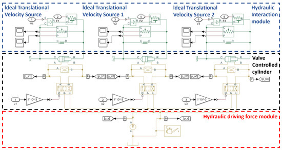
Figure 6.
Hydraulic system’s model in Simulink.

Table 1.
Hydraulic system’s parameter setting for the simulation model.
The physical model is shown in Figure 7. Table 2 displays the primary structural parameters of the physical model of the hydraulic manipulator.
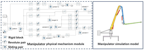
Figure 7.
Physical model of the manipulator in Simulink.
Table 2.
Structure parameters of the simulated mechanical model.
Figure 8 displays the Simulink-built VDC control algorithm model. The whole control algorithm model consisted of four parts, as shown in the following Figure. The output force of the hydraulic cylinder was obtained through kinematics and dynamics calculations by inputting the desired joint angles. The movement of the whole manipulator was controlled by the spool displacement signal of the servo valve.
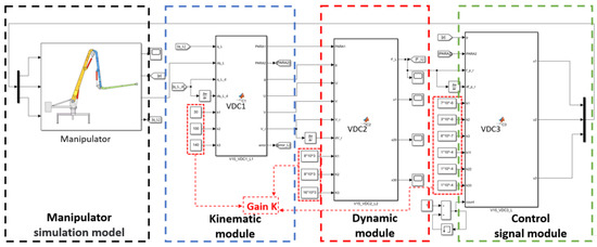
Figure 8.
Simulation model of VDC control algorithm.
6.2. Method Validation in a Simulation without Disturbances
To test the control ability of the proposed method, the valve ports’ flow coefficients and the elastic volume moduli of the servo valves had to be identified first. The flow coefficients and elastic bulk moduli of each valve were identified by the least squares method and Equation (42)–(44). Table 3 shows the results.
Table 3.
Valve ports’ flow coefficient and elastic bulk modulus values.
The triangular trajectory and elliptical trajectory were used in the simulation to verify the control precision of the algorithm. The starting point of the trajectory was set to (1.2 m, 0 m). The running times of the triangular trajectory was 80 s, and that of the elliptical trajectory was 50 s. The sampling interval time was 0.001 s. The PID and MBC control methods were compared with the VDC in the simulation to better illustrate the efficacy of our method. The simulation results are shown in Figure 9. The trajectory curves of the end of the manipulator in the directions X and Y are shown in Figure 9a,b, respectively. Figure 9c–e shows the comparative effect of the angle error of three joints. The comparison of the end position errors is shown in Figure 9f–h. The control of the joint angles’ errors by VDC was superior to that of the other two control algorithms, except for the joint angle 3
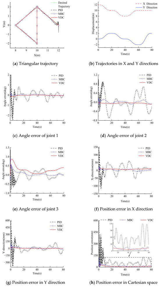
Figure 9.
Simulation results for the VDC control algorithm for a triangular trajectory.
Similarly, a comparison was conducted for the elliptical trajectory, as shown in Figure 10.
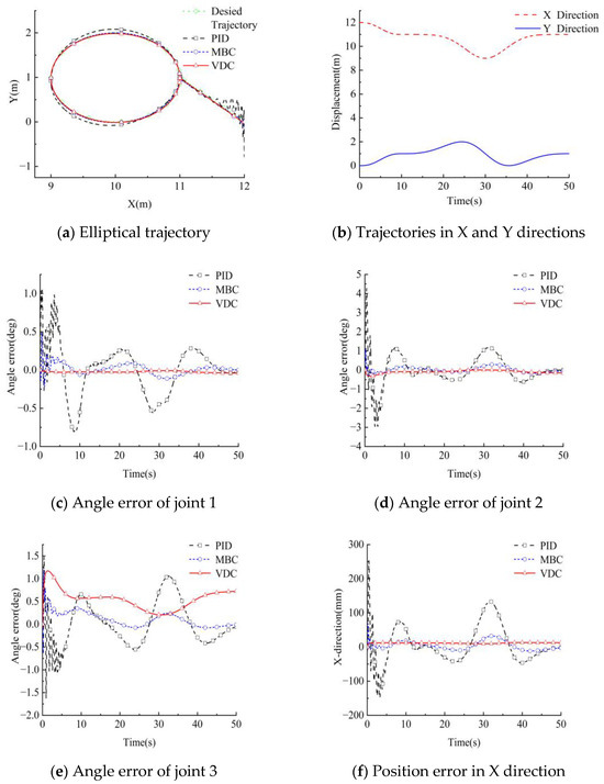
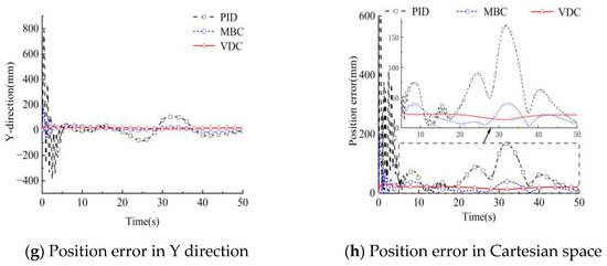
Figure 10.
Simulation results for the VDC control algorithm for an elliptical trajectory.
The control results for the two trajectories are shown in Table 4.
Table 4.
Comparison of the maximum position errors in Cartesian space of the 3 examined methods.
The maximum position errors of the proposed control method were smaller than MBC and PID methods, as shown in Table 4. Compared with PID, the maximum position errors under VDC control were reduced by 113.3 mm and 147.8 mm, corresponding to a decline of 90.4% and 86.3% respectively. MBC showed higher control precision, to a certain extent, than PID. However, the maximum position errors were still further reduced by 3.7 mm and 17.8 mm in the two trajectories when using VDC, with a reduction of 23.6% and 44.3%. Therefore, VDC achieved a high-precision control of the manipulator in an environment without external disturbance. External disturbances were the applied in a simulation to further test the control precision of the proposed method.
6.3. Method Validation in a Simulation with External Disturbances
A straight trajectory was designed from the starting point (The red dot in Figure 11a, position coordinate (12, 0)) to the final point (The gray dot in Figure 11a, position coordinate (10, 2)), and instantaneous disturbances of 1000 N were applied to the tip of the manipulator (tip of link 3) at the 8th and 25th second, as shown in Figure 11a,b. MBC was compared with VDC to better test the control effect, and the results are shown in Figure 11c–f.
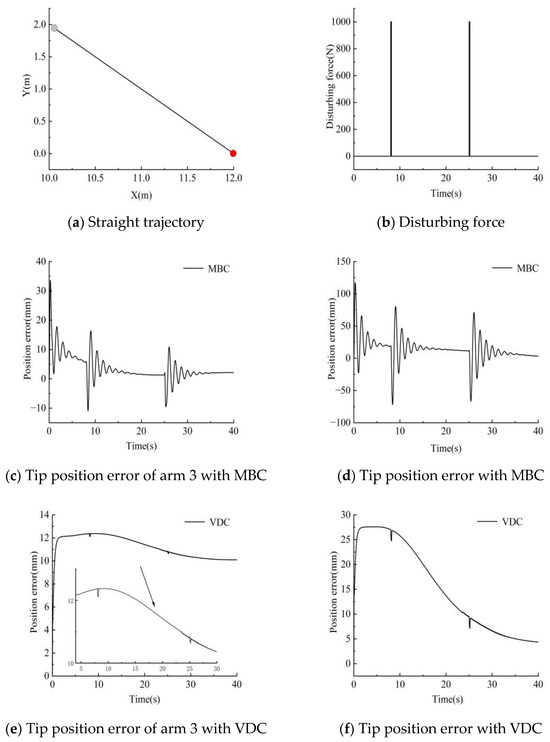
Figure 11.
Simulation results for the VDC control algorithm in the presence of disturbing forces.
As observed in Figure 11c–d, the maximum end position error of arm 3 was 33.4 mm, while the maximum end position error of the manipulator was 117.2 mm when using MBC. As observed in Figure 11e–f, the maximum end error of arm 3 and the overall maximum end error when using the proposed control method were 12.2 mm and 27.5 mm, respectively (the arrow means to point in detail for the part of the influence of disturbances in curve). The position errors were reduced by 63.4% and 76.5%, respectively, compared with the position errors under MBC control. In addition, Figure 10c–f also shows the end amplitudes caused by two external disturbances under different control methods. The two amplitudes under VDC control were 2.4 mm and 2.3 mm, with a decrease of 97.1% and 97.8% compared to the amplitudes of 89.7 mm and 76.1 mm obtained under MBC control.
The effect of an external impact on the motion precision of the manipulator was effectively reduced, which proved the efficacy of the proposed high-precision control algorithm.
7. Discussion
The structure of most hydraulic manipulators is relatively simple, and most of them are driven by hydraulic actuators directly connected to the links. The hydraulic manipulator researched in this paper had a complex structure, with closed chains composed of a link, a luffing mechanism, and a hydraulic actuator. The traditional VDC needs to decompose this complex strongly coupled closed-chain structure several times. Thus, the kinematic derivation of the system would become complicated, and at the same time, the design of the control law would become more difficult. The kinematic features of the luffing mechanism and the arm were treated as equivalent in this paper, avoiding multiple cuts to the complex structure by considering equivalent external forces applied to the hinge points of the two arms. This method reduced the number of subsystems generated and the calculation cost. The simulation results in different environments showed that this method could ensure a high control accuracy while reducing the number of subsystems. All the work in this paper was based on simulation only. A real hydraulic system includes oil viscosity, hydraulic cylinder friction, etc., which may be affected by environmental temperature, humidity, and other factors. The characteristics of the oil flow and the structure of the pipeline limit the dynamic response of the hydraulic system, which could cause a delay in the execution of the control instructions. Future research will attempt to test the proposed control method using a genuine hydraulic manipulator and then refine it in light of the experimental findings.
8. Conclusions
The motion control precision of hydraulic manipulators is difficult to improve due to problems such as structural redundancy, strong coupling in closed-loop structures, and flow/pressure coupling. In this paper, a high-precision motion control method based on VDC is proposed for hydraulic manipulators. The method decomposed the coupled structure into independent and complete subsystems based on the dynamic models of the hydraulic system and the manipulator. The virtual cutting method proposed in this paper could decouple the manipulator with fewer modules compared with the traditional VDC. Avoiding an excessive virtual decomposition of the hydraulic manipulator and requiring fewer model parameters. An adaptive algorithm was used to identify and update the inertial parameters of the manipulator in real time and reduce the influence of the inertial parameters. Finally, a simulation model was established for a 13 m three-degree-of-freedom hydraulic manipulator. Simulations were used to test the efficacy of the control method in various situations. The results showed that the maximum position errors of the proposed control method were reduced by 90.4%, 86.8%, 23.6%, and 44.3% compared with the errors of the PID and MBC methods. The maximum position errors when using VDC in the simulation with external disturbances was reduced by 76.5% compared with that obtained with MBC. The amplitude and the stability time were reduced by more than 97%. Therefore, higher motion control precision can be achieved in hydraulic manipulators with the proposed method.
Author Contributions
Conceptualization, R.D.; methodology, Z.L.; software, Z.L.; validation, Z.L., and Z.D.; formal analysis, G.L.; investigation, R.D.; resources, R.D.; data curation, Z.D.; writing—original draft preparation, Z.L.; writing—review and editing, R.D.; supervision, G.L. All authors have read and agreed to the published version of the manuscript.
Funding
This work was supported by the National Natural Science Foundation of China under grant No. 52175050 and U21A20124; Jiangxi Provincial Natural Science Foundation under grant No. 20212ACB214004 and Key Research and Development Program of Zhejiang Province under grant No. 2022C01039.
Institutional Review Board Statement
Not applicable.
Informed Consent Statement
Not applicable.
Data Availability Statement
Not applicable.
Conflicts of Interest
The authors declare no conflict of interest.
Abbreviations
| Name | Description and Unit |
| VDC | Virtual decomposition control |
| VCP | Virtual cutting point |
| VPF | Virtual power flow |
| MBC | Model-based control |
| CC | Closed chain |
| OC | Open chain |
| v | Linear velocity in the original frame |
| w | Angular velocity in the original frame |
| qi | Joint angle (rad) |
| xi | Displacement of the cylinders (mm) |
| Joint angle velocity (rad/s) | |
| Velocity of the hydraulic cylinder (mm/s) | |
| Required angular velocity (rad/s) | |
| Desired angular velocity (rad/s) | |
| sa | Hydraulic cylinder area with the rod (cm2) |
| sb | Hydraulic cylinder area without the rod (cm2) |
| c | Displacement of the piston rod (mm) |
| ps | System pressure (Mpa) |
| pa | Hydraulic cylinder pressure with the rod (Mpa) |
| Pb | Hydraulic cylinder pressure without the rod (Mpa) |
| E | Bulk modulus (pa) |
References
- Henikl, J.; Kemmetmüller, W.; Bader, M.; Kugi, A. Modelling, simulation and identification of a mobile concrete pump. Math. Comput. Model. Dyn. Syst. 2015, 21, 180–201. [Google Scholar] [CrossRef]
- Luo, S.; Cheng, M.; Ding, R.; Wang, F.; Xu, B.; Chen, B. Human–Robot Shared Control Based on Locally Weighted Intent Prediction for a Teleoperated Hydraulic Manipulator System. IEEE/ASME Trans. Mechatron. 2022, 27, 4462–4474. [Google Scholar] [CrossRef]
- Cheng, M.; Li, L.; Ding, R.; Xu, B. Real-Time Anti-Saturation Flow Optimization Algorithm of the Redundant Hydraulic Manipulator. Actuators 2021, 10, 11. [Google Scholar] [CrossRef]
- Konrad, J.; Morten, K. Development of Point-to-Point Path Control in Actuator Space for Hydraulic Knuckle Boom Crane. Actuators 2020, 9, 27–46. [Google Scholar]
- Chao, Y.; Yujia, W.; Feng, Y. Driving performance of underwater long-arm hydraulic manipulator system for small autonomous underwater vehicle and its positioning precision. Int. J. Adv. Robot. Syst. 2017, 14, 1–18. [Google Scholar]
- Qiao, L.; Zhao, M.; Wu, C.; Ge, T.; Fan, R.; Zhang, W. Adaptive PID control of robotic manipulators without equality inequality constraints on control gains. Int. J. Robust Nonlinear Control 2022, 32, 9742–9760. [Google Scholar] [CrossRef]
- Tan, N.; Li, C.; Yu, P.; Ni, F. Two model-free schemes for solving kinematic tracking control of redundant manipulators using CMAC networks. Appl. Soft Comput. 2022, 126, 109267. [Google Scholar] [CrossRef]
- Hu, S.; Liu, H.; Kang, H.; Ouyang, P.; Liu, Z.; Cui, Z. High Precision Hybrid Torque Control for 4-DOF Redundant Parallel Robots under Variable Load. Actuators 2023, 12, 232. [Google Scholar] [CrossRef]
- Feng, C.; Chen, W.; Shao, M.; Ni, S. Trajectory Tracking and Adaptive Fuzzy Vibration Control of Multilink Space Manipulators with Experimental Validation. Actuators 2023, 12, 138. [Google Scholar] [CrossRef]
- Lee, J.; Chang, P.H.; Yu, B.; Jin, M. An Adaptive PID Control for Robot Manipulators under Substantial Payload Variations. IEEE Access. 2020, 8, 162261–162270. [Google Scholar] [CrossRef]
- Li, S.; He, J.; Li, Y.; Rafique, M.U. Distributed Recurrent Neural Networks for Cooperative Control of Manipulators: A Game-Theoretic Perspective. Appl. Soft Comput. 2022, 126, 109267. [Google Scholar] [CrossRef] [PubMed]
- Mohammad, M.F.; Siamak, A. Discrete adaptive fuzzy control for asymptotic tracking of robotic manipulators. Nonlinear Dynamic. 2014, 78, 2195–2204. [Google Scholar]
- Cho, B.; Kim, S.W.; Shin, S.; Oh, J.H.; Park, H.S.; Park, H.W. Energy-Efficient Hydraulic Pump Control for Legged Robots Using Model Predictive Control. IEEE/ASME Trans. Mechatron. 2023, 28, 3–14. [Google Scholar] [CrossRef]
- Li, J.; Wang, C. Dynamics Modeling and Adaptive Sliding Mode Control of a Hybrid Condenser Cleaning Robot. Actuators 2022, 11, 119. [Google Scholar] [CrossRef]
- Fu, Z.; Junhui, Z.; Min, C.; Bing, X. A Flow-Limited Rate Control Scheme for the Master–Slave Hydraulic Manipulator. IEEE Trans. Ind. Electron. 2022, 69, 4988–4998. [Google Scholar]
- Pang, W.; Chai, Y.; Liu, H.; Li, F. Nonlinear Vibration Characteristics of a Hydraulic Manipulator Model: Theory and Experiment. J. Vib. Eng. Technol. 2023, 11, 1765–1775. [Google Scholar] [CrossRef]
- Park, C.G.; Yoo, S.; Ahn, H.; Kim, J.; Shin, D. A coupled hydraulic and mechanical system simulation for hydraulic excavators. J. Syst. Control Eng. 2020, 234, 527–549. [Google Scholar] [CrossRef]
- Janošević, D.; Pavlović, J.; Jovanović, V.; Petrović, G. A Numerical and Expremental Analysis of The Dynamics Stability of Hydraulic Excavators. Facta Univ.-Ser. Mech. Eng. 2018, 16, 157–170. [Google Scholar]
- Kalmari, J.; Backman, J.; Visala, A. Nonlinear model predictive control of hydraulic forestry crane with automatic sway damping. Comput. Electron. Agric. 2014, 109, 36–45. [Google Scholar] [CrossRef]
- Ruqi, D.; Zhen, W.; Min, C. Model-based Control of the Hydraulic Manipulator for the High-precision Trajectory Tracking. J. Mech. Eng. 2023, 59, 1–12. [Google Scholar]
- Zhou, S.; Shen, C.; Xia, Y.; Chen, Z.; Zhu, S. Adaptive robust control design for underwater multi-DoF hydraulic manipulator. Ocean Eng. 2022, 248, 110822. [Google Scholar] [CrossRef]
- Zheng, X.; Zhu, X.; Chen, Z.; Wang, X.; Liang, B.; Liao, Q. An efficient dynamic modeling and simulation method of a cable-constrained synchronous rotating mechanism for continuum space manipulator. Aerosp. Sci. Technol. 2021, 119, 107156. [Google Scholar] [CrossRef]
- Zhu, W.-H. Virtual Decomposition Control: Toward Hyper Degrees of Freedom Robots; Springer Science & Business Media: Berlin/Heidelberg, Germany, 2010. [Google Scholar]
- Zhu, W.H.; Lamarche, T.; Dupuis, E.; Jameux, D.; Barnard, P.; Liu, G. Precision control of modular robot manipulators: The VDC approach with embedded FPGA. IEEE Trans. Robot. 2013, 29, 1162–1179. [Google Scholar] [CrossRef]
- Koivumäki, J.; Zhu, W.-H.; Mattila, J. Addressing Closed-chain dynamics for high-precision control of hydraulic cylinder actuated manipulators. In Proceedings of the BATH/ASME 2018 Symposium on Fluid Power and Motion Control, Bath, UK, 12–14 September 2018; ASME: New York, NY, USA, 2018; p. V001T01A018. [Google Scholar]
- Koivumäki, J.; Mattilam, J. High performance nonlinear motion/force controller design for redundant hydraulic construction crane automation. Autom. Constr. 2015, 51, 59–77. [Google Scholar] [CrossRef]
- Petrović, G.R.; Mattila, J. Mathematical modelling and virtual decomposition control of heavy-duty parallel–serial hydraulic manipulators. Mech. Mach. Theory 2022, 170, 104680. [Google Scholar] [CrossRef]
Disclaimer/Publisher’s Note: The statements, opinions and data contained in all publications are solely those of the individual author(s) and contributor(s) and not of MDPI and/or the editor(s). MDPI and/or the editor(s) disclaim responsibility for any injury to people or property resulting from any ideas, methods, instructions or products referred to in the content. |
© 2023 by the authors. Licensee MDPI, Basel, Switzerland. This article is an open access article distributed under the terms and conditions of the Creative Commons Attribution (CC BY) license (https://creativecommons.org/licenses/by/4.0/).