Rate-Dependent Hysteresis Model of a Giant Magnetostrictive Actuator Based on an Improved Cuckoo Algorithm

Abstract

A rate-dependent asymmetric Prandtl–Ishilinskii (RAPI) model was proposed to tackle the serious rate-dependent hysteresis nonlinearity of the giant magnetostrictive actuator(GMA) output. First, a polynomial function was introduced based on the PI model, and hysteresis factors were introduced to the Play operator, which accurately described the asymmetrical characteristic of the actuator output. On this basis, rate-dependent parameters were added to establish a rate-dependent RAPI model. Second, an improved cuckoo search (ICS) algorithm was proposed to solve the difficulty in the parameter identification of the RAPI model. For the ICS algorithm, the algorithm stability and optimization accuracy were improved using the adaptive step (AS) strategy and bird’s nest disturbance strategy. Then, the effectiveness of the ICS algorithm was tested by comparing it with other parameter identification algorithms. Finally, the rate-dependent RAPI model was verified by combining the output data of the giant magnetostrictive actuator under different frequencies. The results show that the rate-dependent RAPI model exhibits a higher accuracy than the PI model, thus verifying the effectiveness of the rate-dependent RAPI model.

1. Introduction

A giant magnetostrictive actuator, a new-type actuator with giant magnetostrictive materials as the drive element, is a power output device with the magnetostrictive effect, accompanied by the advantages of a high output frequency, strong stability, and large output force [1]. In recent years, the increasing speed of high-speed trains has increased the vibration of the train due to the irregularities of the track. The application of a giant magnetostrictive actuator to a train’s active suspension allows for different damping forces to be output based on the disturbance excitation of distinct lines, thereby lessening train vibration and enhancing the stability and comfort of the train operation. Therefore, the application of a super magnetostrictive actuator in train active suspension has a good prospect.

Due to the serious hysteresis nonlinearity of the giant magnetostrictive actuator output, however, it is difficult to control the precise output, which greatly limits the practical application of giant magnetostrictive actuators [2]. The hysteresis characteristic of a giant magnetostrictive actuator can be expressed by a hysteresis model, and establishing an accurate hysteresis model has become a significant foundation for solving hysteresis nonlinearity. At present, hysteresis models are generally divided into two types: physical models and phenomenological models, the former of which mainly include the J-A model [3] and the free energy model [4] and the latter of which include the Preisach model [5], the Prandtl–Ishilinskii (PI) model [6], and neural network models [7]. In application, the J-A model and the free energy model require high-precision experimental data and more model parameters. The Preisach model is characterized by dual integrals and a complicated solving process, thus restricting its application. The solution precision of neural network models excessively relies upon the accuracy of experimental data. Over the other methods, the PI model integrates the advantages of a small calculated quantity, high flexibility, and easy identification and solution. In this study, therefore, a giant magnetostrictive actuator was subjected to hysteresis modeling based on the PI model.

The PI model was put forward by Prandtl et al. to model magnetic materials. In the process of popularization, the basic PI model has been improved by research scholars and applied in various fields. Zhong, Y. [8] introduced a cubic polynomial into the primary function of the PI model to construct an enhanced PI model, endowing the model with asymmetry so that it could describe the magnetic hysteresis phenomenon within a wider range and identify model parameters using the moth–flame algorithm. The results showed that the fitting accuracy of the improved PI model is significantly higher than that of the classical PI model under high frequencies. Zhao, X.H. [9] divided hysteresis nonlinearity into a linear module and a nonlinear model, described the nonlinear model with the PI model, replaced the linear model with an electromechanical transfer function, and finally connected the PI model with the transfer function in series to form a dynamic hysteresis model and solve the inverse model. The results manifested that the designed dynamic PI model displays good performance within 0–50 Hz. Tang, H.B. [10] improved the PI model by adding a dead-zone operator and introducing a frequency function. It was then experimentally verified that the improved model is much better than the classical PI model and can fit the GMM output curve well within 80 Hz. Pan, Y. [11] optimized the parameters of the classical PI model using the sequential quadratic programming algorithm, added a shift operator to make the model asymmetric, and improved the rate dependence of the model through the series ARX model given the shortcomings of the asymmetric PI model. Finally, it was verified that the model has a good fitting effect on hysteresis curves above 200 Hz, but the improving effect on low-frequency hysteresis curves is not evident. Subhash Rakheja et al. [12] established a rate-dependent PI model based on the memoryless function of the dead-zone operator and compared the comprehensive PI model data and the actual output. The comparison results revealed that the improved model can describe the nonlinear hysteresis characteristics in a wide range of excitation amplitudes and frequencies. Dargahi et al. [13] described the hysteresis curve of the magnetorheological elastomer using the improved generalized PI model and replaced the original equal interval distribution with the threshold distribution function. The results showed that the improved generalized model can accurately characterize the hysteresis characteristics of magnetorheological materials under different loading conditions and magnetic field ranges. Peng et al. [14] applied the PI model to the hysteresis nonlinear modeling of a giant magnetostrictive actuator, proposed a rate-dependent modified PI model, and then identified the parameters of the model by using the constrained least squares method. The results showed that, within a certain frequency range, the rate-dependent modified PI model could effectively describe the hysteresis characteristics of the giant magnetostrictive actuator. Xiao et al. [15] modified the classical PI model and used the least square method to identify parameters of the modified PI model. The results show that the modified PI model can reduce the modeling error, but the model accuracy is still not guaranteed under a high frequency. Nie, L.L. et al. [16] established a rate-dependent asymmetric hysteresis RDAPI model by introducing a dynamic envelope function into the play operator of the PI model and then combined with other improved PI models to characterize the rate-dependent and asymmetric hysteresis behavior of the piezoelectric micro-positioning level. Experiments show that the accuracy of the RDAPI model is improved significantly. On this basis, a robust adaptive control method is proposed. Wang, W. et al. [17] improved the Play operator in the PI model to an asymmetric operator, established an asymmetric API model, and optimized the parameters of the API model, which reduced the number of parameters and maintained a high accuracy. The experimental results show that the compensator based on this model can effectively suppress the hysteresis of the piezoelectric actuator.

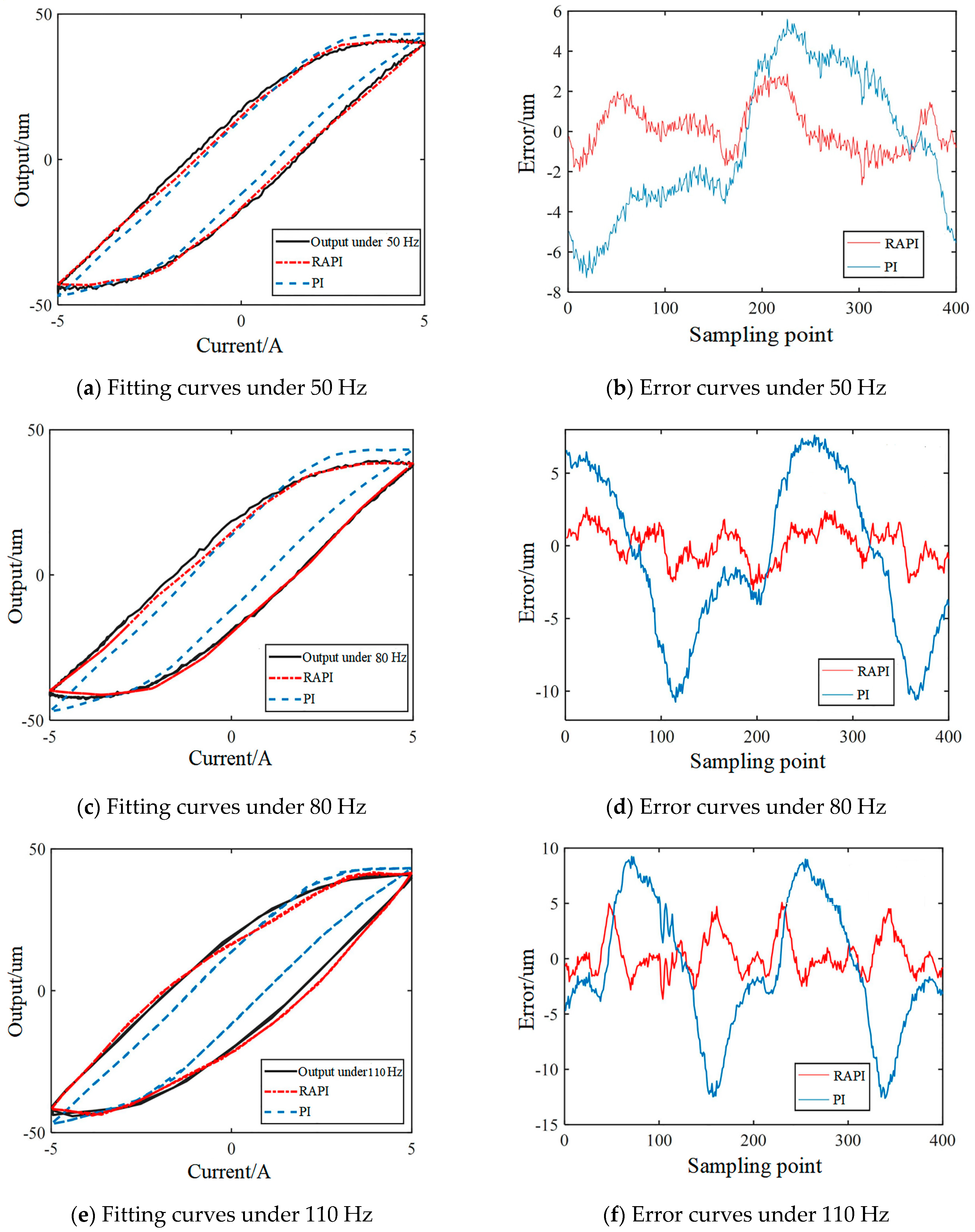
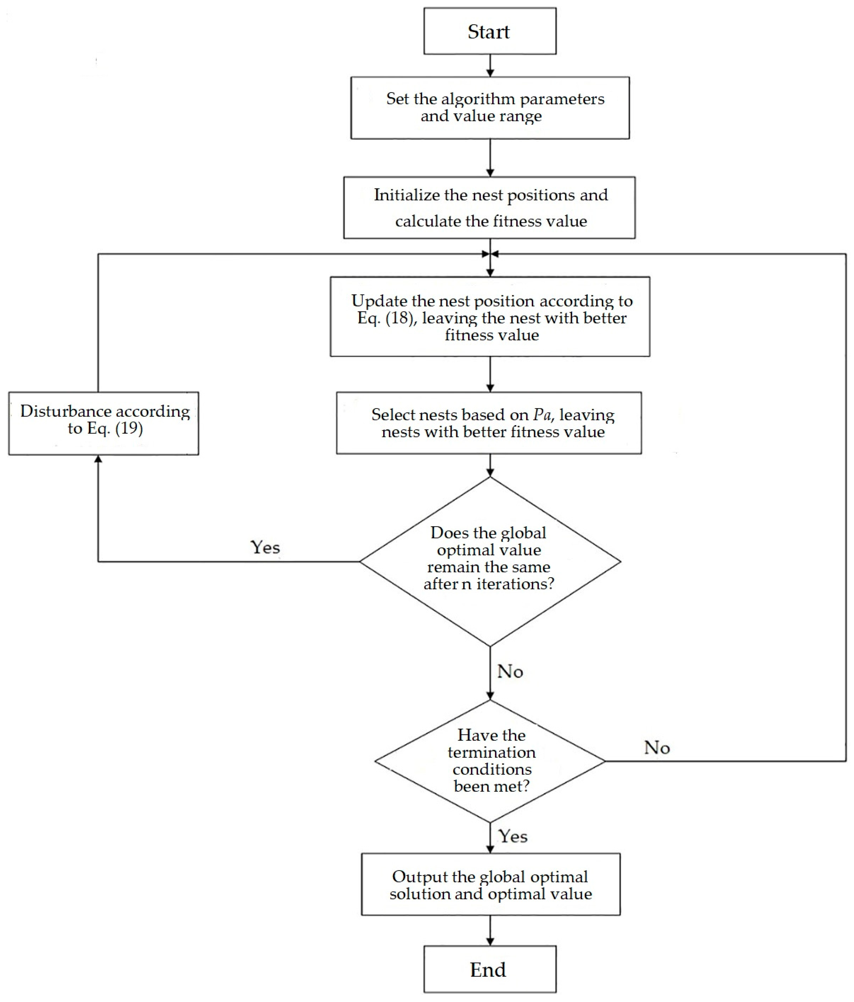
In summary, the parameter identification and hysteresis modeling techniques for the magnetostrictive actuator based on the PI model are still immature. In this paper, aiming at the rate-dependent asymmetric hysteresis characteristics of the output curve of the active suspension magnetostrictive actuator, a rate-dependent asymmetric PI (RAPI) model was constructed by adding auxiliary functions based on the PI model, which can accurately describe the hysteresis curve of the output of the magnetostrictive actuator. In order to solve the problem of the RAPI model having multiple parameters that are difficult to identify, an improved cuckoo search (ICS) algorithm was proposed, which has higher optimization accuracy and stability compared to traditional algorithms. Finally, through comparative experiments with the PI model, it is verified that the RAPI model effectively improves the fitting accuracy of the actuator’s hysteresis curve. Based on the RAPI model, precise dynamic control of the giant magnetostrictive actuator can be further achieved, which is of great significance for the practical application of the magnetostrictive actuator in the active suspension of trains.

2. Rate-Dependent Asymmetric PI Model

2.1. PI Model

In the PI model, the hysteresis of the output is generally described by the weighted superposition of the Play operator [18]. The basic Play operator is defined as follows: C_m [0,t_E] is assumed to be the set of all continuous piecewise functions in the definitional domain of [0,t_E], in which 0 = t₀ < t₁ < t₂… < t_E, u(t)∈C_m, and the output of the Play operator is:

$$F_r\left[u\left(0\right)\right]=f_r\left(u\left(0\right),0\right)$$

(1)

$$F_r[u(t)]=f_r\left(u(t),F_r[u(t-1)]\right)$$

(2)

$$f_r(u(t),F_r[u(t-1)])=\max \{u(t)-r,\min (u(t)+r,F_r[u(t-1)])\}$$

(3)

Here, F_r [u(0)] is the output of a single Play operator at the initial moment; F_r [u(t)] denotes the output of a single Play operator at time t, in which u(t) stands for the input signal at time t; F_r [u(t − 1)] represents the output of the Play operator at the time before t. r is the threshold of the Play operator.

The output of the PI model is obtained through the weighted superposition of multiple Play operators with different thresholds and the summation with the input linear function, with the following output formula:

$$PI(t)=\alpha u(t)+{\displaystyle \sum _{i=1}^n{P}_{ri}}{F}_{ri}\left[u\right](t)$$

(4)

Here, PI(t) is the output of the PI model; u(t) denotes the input of the PI model; α is the weight of the input; n represents the number of Play operators in the PI model; P_ri stands for the weight of each Play operator.

2.2. Asymmetric PI (API) Model

The Play operator of the PI model is centrosymmetric, and the output of giant magnetostrictive actuators is characterized by asymmetric hysteresis, leading to a big error in the description of the asymmetric hysteresis curve by the PI model. Therefore, the PI model should be improved to make up for this deficiency. If introduced into the PI model, high-order polynomials, which are generally asymmetric, can endow the model with the ability to fit asymmetric curves. In this study, the linear function in the PI model was substituted by a polynomial function as follows:

$$G\left[u\left(t\right)\right]=a_0+a_{1}u\left(t\right)+a_{2}u{\left(t\right)}^2+a_{3}u{\left(t\right)}^3+a_{4}u{\left(t\right)}^4+\dots a_{n}u{\left(t\right)}^n$$

(5)

Despite the asymmetry of the model output thanks to the polynomial function, the model details were not described, so the hysteresis factor β was introduced into the model to optimize the operator Play. The improved expression is as follows:

$$F_{r,\beta }\left[u\left(t\right)\right]=\max \{u(t)-\beta r,\min (u(t)+\beta r,F_{r,\beta }[u(t-1)])\}$$

(6)

Here, F_r,_β[u(t)] is the output of the improved Play operator at the current moment; F_r,_β [u(t − 1)] stands for the output of the operator at the previous moment. The value of β could change the output amplitude and output gap of the Play operator, thus affecting the output of the asymmetric PI model. With the above improvements combined, the asymmetric PI model is expressed as shown in Formula (7).

$$API\left[u\left(t\right)\right]=G\left[u\left(t\right)\right]+{\displaystyle \sum _{i=1}^n{P}_{ri}}{F}_{ri,\beta i}\left[u\left(t\right)\right]$$

(7)

2.3. RAPI Model

A study [19] has shown that when the excitation frequency is greater than 5 Hz, the hysteresis characteristics of giant magnetostrictive actuators will be affected by the frequency, showing rate-dependent hysteresis characteristics. Since the PI model is rate-independent, and neither the added hysteresis factor nor the auxiliary function contain frequency parameters, rate dependence processing is required for the asymmetric PI model.

The current rate-dependent hysteresis modeling methods can be divided into two types: separated rate-dependent hysteresis models and overall rate-dependent hysteresis models. The separated rate-dependent hysteresis models divide the hysteresis nonlinearity of the system into rate-independent hysteresis links of giant magnetostrictive materials and linear time invariant links consisting of other components, which are then respectively modeled and connected in series so as to establish an integral system model. Overall rate-dependent hysteresis models do not differentiate the system and establish a holistic model. Given that the model accuracy of separated modeling will be reduced under the high input frequency, the asymmetric PI model was improved in terms of the aspect of rate dependence through the overall modeling method. Moreover, the coefficient c of the weighted Play operator sum was added, and a frequency function specific to the auxiliary function G[u(t)] and the hysteresis factor β was constructed:

$$RAPI\left[u\left(t\right)\right]=G_f\left[u\left(t\right)\right]+c\left(f\right){\displaystyle \sum _{i=1}^n{P}_{ri}}{F}_{ri,}{\beta }_{ri\left(f\right)}\left[u\left(t\right)\right]$$

(8)

$$G_f\left[u\left(t\right)\right]=a_0\left(f\right)+a_1(f)u\left(t\right)+a_2\left(f\right)u{\left(t\right)}^2+a_3\left(f\right)u{\left(t\right)}^3+\cdots +a_n\left(f\right)u{\left(t\right)}^n$$

(9)

$$F\left(f\right)=k_{1,n}\times f+k_{2,n} n=c,\beta ,a_1,a_2,\dots a_n$$

(10)

Here, c(f), β(f), a₀(f)… a_n (f) denote frequency-related parameters. The parameter values were identified by combining the output under different frequencies, and the unknown parameters in Formula (9) were acquired through curve fitting. Then, each frequency function was substituted into Formula (8) so as to obtain the rate-dependent RAPI model.

3. Improved CS Algorithm

3.1. CS Algorithm

With the development of meta-heuristic optimization algorithms in recent years, such new-type optimization algorithms as the artificial fish swarm algorithm [20], CS algorithm [21], and grey wolf algorithm [22] have been developed by researchers and gradually applied to the field of parameter identification [23,24]. Therein, the CS algorithm has been widely used by virtue of a few control parameters and a strong global optimization ability. The CS algorithm is a meta-heuristic optimization algorithm proposed by Yang et al., imitating the predation (Levy flight) and brooding behavior (discovery probability (Pa)) of cuckoos. The algorithm assumes the following conditions for simulation:

• There was only one bird egg in each nest, and the eggs were randomly distributed.
• In each evolution, the bird egg with the highest fitness was reserved.
• Under a fixed number of bird’s nests, the host bird abandoned the cuckoo eggs at Pa, and the eliminated nests would be replaced by new nests.

Based on the above assumptions, the iterative formula for the CS algorithm is as follows:

$$X_i^{\left(t+1\right)}=X_i^t+\alpha \otimes Levy\left(\lambda \right)$$

(11)

$$\alpha ={\alpha }_0\times \left(X_i^t-X_{best}^t\right)$$

(12)

Here, ${ X}_i^{(t+1)}$ is the position of the i-th bird’s nest in the t + 1 iteration; $X_i^t$ stands for the position of the i-th bird’s nest in the t-th iteration; $X_{best}^t$ represents the best bird’s nest for the t-th iteration; α is the factor that controls the step of cuckoo movement, usually taken as 0.01; ⨂ is the product of vectors; Levy(λ) is a random number that obeys the Levy distribution, which is solved by the following formula:

$$Levy\left(\lambda \right)=\frac{\Phi \times \mu }{{\left|\nu \right|}^{1/\beta }}$$

(13)

Here, μ~N(0,1), ν~N(0,1), β was taken as 1.5, Φ through the following formula:

$$\Phi ={\left[\frac{\tau \left(1+\beta \right)\sin \left(\frac{\pi \times \beta }{2}\right)}{\beta \tau \frac{1+\beta }{2}\times 2^{\frac{\beta -1}{2}}}\right]}^{\frac{1}{\beta }}$$

(14)

Here, τ is the standard Gamma function. Based on the above formula, the formula of the CS algorithm is as follows:

$$X_i^{\left(t+1\right)}=X_i^t+{\alpha }_0\times \frac{\Phi \times \mu }{{\left|\nu \right|}^{\frac{1}{\beta }}}\times \left(X_i^t-X_{best}^t\right)$$

(15)

When the bird’s nests were updated according to Levy flight, the host bird would still abandon some nests as per Pa if it found the cuckoo’s eggs, and a random number distributed in [0, 1] was generated through the rand function and compared with Pa. Stochastically biased walk was adopted for the nests whose random number was greater than Pa, while the nests satisfying < Pa were kept unchanged. The random preference formula is as follows:

$$X_i^{t+1}=X_i^t+r\left(X_j^t-X_k^t\right)$$

(16)

$X_j^t$ and $X_k^t$ are two random nests of the t-th generation, and r is a random number following a normal distribution.

The Cuckoo Search algorithm has a simple iterative process and a small number of control parameters. However, it also has limitations: the step size and discovery probability during the optimization process remain constant, which leads to the inability of the Cuckoo Search algorithm to balance global search and local exploration. For complex problems, it cannot rely on Levy flights to escape from local optima.

3.2. CS Algorithm Optimization

3.2.1. Adaptive Step (AS) Strategy

In the CS algorithm, α is the step coefficient, which directly determines the flight distance of the bird’s nest in each iteration. Since α is taken as 0.01 in the standard CS algorithm, the flight distance of the bird’s nest is relatively fixed, resulting in an imbalance between global search and local development. By analyzing the step formula, it can be concluded that under a rather lower α value, the iteration range of the algorithm is small, accompanied by a high search accuracy and a low convergence rate. When the α value is rather higher, the iterative step of the algorithm increases, along with an enlarged search scope and low convergence accuracy [25]. Based on the above analysis, an AS function was proposed in this study and substituted into the following formula:

$$w=2\times (-\frac{w_{\max }-w_{\min }}{K_{\max }}\times K)+\frac{w_{\max }-w_{\min }}{\frac{K}{K_{\max }}+{\exp }^{(-\frac{12\times K}{K_{\max }}-6)}}+w_{\max }$$

(17)

$$X_i^{(t+1)}=X_i^t+w\times \alpha \otimes Levy\left(\lambda \right)$$

(18)

According to the experiment, w_min = 0.8 is the minimum value of the inertia factor; w_max = 2 is the maximum value of the inertia factor; K is the number of iterations; and K_max is the maximum number of iterations, which was set to K_max = 1000. The change in the w value is displayed in Figure 1:

After the AS function was introduced, the algorithm was able to search globally at a large step in the initial stage of iterations and search locally at a small step in the later stage, showing an initially declining, then rising, and finally declining trend on the whole. This not only conformed to the algorithm optimization law but also contributed to the strong population diversity of the algorithm in the middle and later stages.

3.2.2. Bird’s Nest Disturbance Strategy

Although the standard CS algorithm can jump out of the local optimal solution to a certain extent with the help of the Levy flight strategy in the later iteration, a long-step flight is carried out after repeated small-step iterations so that the algorithm cannot get rid of the local optimum in the later iterations. Hence, a bird’s nest disturbance strategy was proposed to disturb the population with abnormal monitoring results by monitoring the results of each iteration.

The specific implementation steps are as follows: The bird’s nests that kept the global optimal solution unchanged in repeated iterations were recorded. When the global optimal solution was unchanged in the n-th iteration of the bird’s nests, the current population was trapped in local optima, so it was disturbed at a disturbance step, which was the linear difference between the optimal solution of the current generation and the position of the bird’s nest. In this way, the algorithm was capable of optimization near the local optimal solution, ensuring that the algorithm could still remain convergent after the disturbance. The disturbance step length formula is as follows:

$$V_{i,j}={\zeta }_1\times ({\zeta }_{2}gbest-X_{i,j})$$

(19)

$${\zeta }_1=s-\frac{s\times i}{N}$$

(20)

Here, $V_{i,j}$ is the j-th dimensional disturbance step in the i-th cuckoo nest; ${\zeta }_1$ is the step factor controlling the disturbance radius, in which I is the current population number; N is the maximum population number; s is a constant; ${\zeta }_2$ stands for the weight coefficient of the contemporary optimal cuckoo nest, taken as 0.03; $X_{i,j}$ is the j-th dimensional nest value in the i-th nest. The disturbance step $V_{i,j}$ was dynamically adjusted by the cuckoo population number $V_{i,j}$, and the disturbance step factor of the head population was large, which enabled the algorithm to perform optimization in a larger scope. The disturbance step factor of the rear population was small, so the algorithm searched near the local optimal solution. The bird’s nest disturbance strategy imposed different disturbance steps on different populations, which facilitated global search and local development with the local optimal solution as the center and effectively improved the optimization accuracy and search ability of the algorithm.

3.2.3. ICS Algorithm Flow

The algorithm flow is as follows.

Step1: Input the algorithm iteration number K_max, the number of nests N, w_max, and w_min.

Step2: Initialize the nest positions and calculate the fitness value.

Step3: Update the nest positions using dynamic inertia Levy flight and retain nests with better fitness.

Step4: Select nests based on Pa, leaving nests with a better fitness value. Calculate the global optimal solution and the fitness value of the optimal solution.

Step5: Determine whether to disturb the population based on the number of repetitions of the global optimum in each iteration.

Step6: Determine whether the algorithm reaches the termination condition; if not, go back to Step3; when the termination condition is reached, output the optimal solution and the fitness value.

The flowchart of the algorithm is shown in Figure 2:

3.3. Performance Test of the ICS Algorithm

A set of mixed test functions was selected to verify the performance of the ICS algorithm. In the set, functions F1–F3, which are unimodal functions, could test the convergence ability and optimization speed of the algorithm. Functions F4–F6, which are multimodal functions with increasing test difficulties, a large scope of optimization, and multiple local optimal values in the definitional domain, were applied to test the optimization ability of the algorithm for multimodal complex functions. Function F7, a two-dimensional function, was used to test the optimization ability of the algorithm for low-dimensional problems. The expressions of such test functions are listed in

Table 1. Test functions.

Function	Expression	Definitional Domain	Optimal Value
F1	$f\left(x\right)={\displaystyle \sum _{i=1}^n{x}_i^2}$	[−100, 100]	0
F2	$f\left(x\right)={\displaystyle \sum _{i=1}^n\left|x_i\right|}+{\displaystyle \prod _{i=1}^n\left|x_i\right|}$	[−10, 10]	0
F3	$f\left(x\right)={\displaystyle \sum _{i=1}^{n}i{x}^4}$	[−1.28, 0.64]	0
F4	$f\left(x\right)=\frac{1}{4000}{\displaystyle \sum _{i=1}^n{x}_i^2-{\displaystyle \prod _{i=1}^n\cos \left(\frac{x_i}{\sqrt{i}}\right)}}+1$	[−600, 600]	0
F5	$f\left(x\right)=-20\exp \left[-0.2\sqrt{\frac{1}{n}{\displaystyle \sum _{i=1}^n{x}_i^2}}\right]-\exp \left[\frac{1}{n}{\displaystyle \sum _{i=1}^n\cos \left(2\pi x_i\right)}\right]$	[−10, 10]	0
F6	$f\left(x\right)={\displaystyle \sum _{i=1}^n\left|x_i\sin \left(x_i\right)+0.1x_i\right|}$	[−10, 10]	0
F7	$f\left(x\right)=0.5+\frac{{\sin }^2\left(x_1^2-x_2^2\right)-0.5}{{\left[1+0.001\left(x_1^2+x_2^2\right)\right]}^2}$	[−100, 100]	0

.

The ICS algorithm was comparatively analyzed with particle swarm optimization (PSO), CS, and ASCS to explore its accuracy and convergence.

Table 2. Parameters of test algorithms.

Algorithm	Parameter
PSO	c1 = 1.5, c2 = 1.5, w = 0.5
CS	Pa = 0.25, a = 0.01
ASCS	Stepmin = 0, Stepmax = 0.01, Pa = 0.25

gives the specific parameter settings of each algorithm. The number of test populations was set to 50, the number of dimensions was set to 30, and the maximum number of iterations was set to 1000. Each test function was run 30 times in the same environment, and their average function error (Mean), standard deviation (Std), and optimal value (Best) were recorded. The test results are shown in

Table 3. Experimental result of test functions.

Function	Mean/Std/Best	PSO	CS	ASCS	ICS
F1	Mean	8.92	3.46 × 10−5	5.21 × 10−9	0.00
	Std	3.18	7.20 × 10−10	2.85 × 10−8	0.00
	Best	4.42	5.94 × 10−6	4.52 × 10−267	0.00
F2	Mean	3.51 × 10	3.48 × 10−2	2.07 × 10−2	0.00
	Std	1.07 × 10	8.58 × 10−4	7.40 × 10−2	0.00
	Best	1.96 × 10	2.12 × 10−2	8.53 × 10−3	0.00
F3	Mean	3.18	1.06 × 102	7.13 × 10−16	0.00
	Std	2.29	3.68 × 10	3.90 × 10−15	0.00
	Best	3.17 × 10−1	3.98 × 10	0.00	0.00
F4	Mean	2.26 × 10	8.79 × 10−2	8.30 × 10−4	0.00
	Std	6.55	4.00 × 10−2	4.55 × 10−3	0.00
	Best	1.13 × 10	2.20 × 10−2	0.00	0.00
F5	Mean	1.18 × 10	1.90	8.60 × 10−4	8.88 × 10−16
	Std	1.12	3.93 × 10−1	4.71 × 10−3	0.00
	Best	9.41	1.19	4.44 × 10−15	8.88 × 10−16
F6	Mean	1.52 × 10	7.17	6.93 × 10−1	0.00
	Std	3.46	9.83×10−1	2.29	0.00
	Best	8.46	5.16	3.88 × 10−11	0.00
F7	Mean	1.56 × 10−14	1.57 × 10−6	7.10 × 10−9	0.00
	Std	5.79 × 10−14	1.83 × 10−6	1.96 × 10−8	0.00
	Best	0.00	0.00	0.00	0.00

.

It could be seen that in functions F1–F3, the ICS algorithm could accurately converge to the global optimum. F4, a complex multimodal function, exhibited a lot of local optimal values in the definitional domain. As shown in

Table 4. The expression of the evaluation index.

Evaluation Index	Expression
RMSE	$RMSE=\sqrt{\frac{{{\displaystyle \sum _{i=1}^N\left(c_{\exp }^i-c_{mx}^i\right)}}^2}{N}}$
MAE	$MAE=\frac{1}{N}{\displaystyle \sum _{i=1}^N\left|c_{\exp }^i-c_{mx}^i\right|}$
MAD	$MAD=\underset{1\le i\le N}{\max }\left|c_{\exp }^i-c_{mx}^i\right|$

and

Table 5. Comparison of errors under different numbers of hysteresis factors.

Number of β	RMSE	MAE	MAD
1	0.48	0.29	0.6
2	0.52	0.36	0.7
5	0.68	0.81	2.2
10	0.84	1.02	2.7

, the ASCS algorithm was subjected to a too-large standard deviation and unstable optimization results despite the ability to search the optimal value of F4, while other algorithms all failed to search the global optimal value. The ICS algorithm could converge to the global optimum even after repeated tests. F5 and F6, which were classical complex functions, were featured with a relatively high optimization difficulty. For F6, the ICS algorithm was stuck in the local optimal value of 8.88 × 10⁻¹⁶ in the later stage of iterations, but its optimization accuracy remained higher than that of other algorithms. For F7 (a simple low-dimension function), the ICS algorithm and other algorithms converged to the global optimum, indicating its excellent optimization ability on low-dimension functions. According to the Std value, the standard deviation of the ICS algorithm was 0 in many tests under different functions, manifesting its favorable stability in optimization.

4. Parameter Identification and Experimental Verification of the RAPI Model

4.1. Parameter Optimization

The RAPI model was established on the basis of the API model, the parameters of which, therefore, were identified first. Some parameters preset in the API model were optimized.

4.1.1. Optimization of the Number of Hysteresis Factors

Hysteresis factors could change the shape of the Play operator by influencing the threshold so as to generate an impact on the output, and the model will be affected, to different degrees, by the number of hysteresis factors. Different quantities of hysteresis factors were thereby experimented, and the maximum absolute deviation (MAD), the mean absolute error (MAE), and the root mean square error (RMSE) were used as evaluation indexes for the model fitting accuracy, as shown in Table 4.

Combining the displacement data of the sinusoidal current under the amplitude of 2 A and 10 Hz, the parameters of four schemes were identified, respectively. The number of operators was set to 10, the order of the auxiliary function was set to 3, and the rest of the parameters were obtained through the ICS algorithm. Table 5 presents the evaluation results under four different numbers of hysteresis factors. As the number of hysteresis factors increased, the model fitting error gradually increased, so the number of hysteresis factors was set to 1 in this study.

4.1.2. Order Optimization of the Auxiliary Function

The auxiliary function in the API model is the key factor deciding the model asymmetry, and its order affects the complexity of the model and the difficulty in parameter identification. Therefore, it was necessary to optimize the model order. An experiment was carried out through the control variable method to acquire the optimal number. Therein, the number of operators was set to 10, that of hysteresis factors was set to 1, the polynomial order was set to 1–6, and the other parameters were determined through the relevant parameter identification algorithm.

It could be observed from Figure 3 that the RMSE decreased considerably when the order of the auxiliary function increased from one to three and basically kept unchanged as the order grew from three to four, but it rose again when the order increased to five and six. This is because the increase in the function order aggravates the difficulty in parameter identification and leads to the failure to converge to the global optimum after reaching the given number of iterations. Moreover, the parameter identification time is substantially lengthened as the model order increases. In full consideration of the model accuracy and parameter identification time, the order of the auxiliary function was chosen to be three, expressed in Formula (20).

$$G\left[u\left(t\right)\right]=a_0+a_{1}u\left(t\right)+a_{2}u{\left(t\right)}^2+a_{3}u{\left(t\right)}^3$$

(21)

4.1.3. Optimization of the Number of Play Operators

As the basic operation unit of a hysteresis model, the Play operator plays an important role in the model output. The model fitting accuracy will decline under a small number of operations. A too-large number of operations will intensify the complexity of the calculation though improve the prediction accuracy to some extent. To determine the concrete number of operators, the experiment was carried out under different numbers of operators, with other parameters remaining the same. Figure 4 shows the RMSE curve under different numbers of operators. With the increase in the number of operators, the RMSE gradually decreased, indicating that the fitting accuracy of the model is gradually improved. The subsequent increase in the number of operators >10 generated a very minor influence on the RMSE. Hence, the number of operators was determined to be 10 to balance the prediction accuracy and the complexity of the calculation.

4.2. Parameter Identification of the RAPI Model

4.2.1. Parameter Identification of the API Model

In this study, the model parameters were identified by combining the experimental data under the current amplitude increasing in the range of 1–5 A and the frequency of 1 Hz. In this process, the number of populations of the ICS algorithm was set to 80, the maximum number of iterations was set to 1000, and the disturbance threshold was set to 3. In the PI model, the weight value was generally positive, but it was experimentally found that a lower RMSE could be acquired when the weight value was negative, so a negative weight value could be assigned to the API model. Since the API model is the sum of the weighted superposition of Play operators, the model characteristics would not be changed by a small number of negative values. The ICS algorithm was repeatedly run ten times, the optimal value and the optimal bird’s nest were recorded, and the API model parameters finally obtained are listed in

Table 6. Parameter identification results of the API model.

Operator No.	Threshold	Weight
0	0	2.2526
1	0.5	2.2068
2	1	1.7295
3	1.5	2.4370
4	2	1.8501
5	2.5	0.6715
6	3	−0.0693
7	3.5	0.3086
8	4	0.2692
9	4.5	0.2779

and

Table 7. Hysteresis factors and auxiliary coefficients of the API model.

Parameter	Value
β	1.0056
a0	0.2699
a1	2.7287
a2	−0.2615
a3	−0.0547
c	1

.

4.2.2. Parameter Identification of the RAPI Model

On the basis of the API model, the rate-related parameters were identified. To reduce the influence of environmental noise on the test displacement as much as possible, the other model parameters were experimentally identified by selecting the sinusoidal current with an amplitude of 5A, the signals with the frequency of [1,25,40,55,70,85,100,120], and the Play operators with a constant weight value.

Table 8. Parameter values of the RAPI model under different frequencies.

Frequency	β	α3	α2	α1	α0	c
1	0.9739	−0.0681	−0.0249	2.0342	−0.1091	1
25	0.9872	−0.0616	−0.0214	1.2331	0.0429	1.2192
40	1.0198	−0.0557	−0.0169	−0.0524	0.3016	1.3033
55	1.0321	−0.0429	−0.0141	−0.0524	0.3016	1.3615
70	1.0472	−0.0384	−0.0115	−1.261	0.6109	1.4099
85	1.048	−0.0309	−0.0095	−2.9429	0.7222	1.4637
100	1.0904	−0.0308	−0.0064	−3.1027	0.8558	1.4659
120	1.1193	−0.0185	−0.0009	−4.543	1.2016	1.6500

shows the values of the model coefficients at different frequencies obtained by the parameter identification algorithm.

4.3. Verification of the RAPI Model

In order to obtain the hysteresis input–output data required for the identification model, a giant magnetostrictive actuator test bench is built, as shown in Figure 5. The experimental bench mainly includes: the giant magnetostrictive actuator, YB1635 signal generator, NI-usb6211 acquisition card and display device, Aigtek-ATA309 power amplifier, Panasonic HG-C1030 laser displacement sensor, and PC and Tektronix-MDO3014 oscilloscope. Among them, the signal generator generates a positive rotating AC signal, which is amplified by the power amplifier to drive the vibration of the super magnetostrictive actuator with a suitable excitation current. The laser displacement sensor, oscilloscope, acquisition card, and display device cooperate with the PC to complete the display, acquisition, processing, and post-analysis of data.

The experimental curves at 50, 80, and 110 Hz were randomly selected and compared with the curves acquired by the PI model and the RAPI model. The fitting error curves of the two models are shown in Figure 6. It could be observed from the fitting curves of the two models that the RAPI model curves introduced with a frequency function could accurately fit the hysteresis curve of the giant magnetostrictive actuator at variable frequencies. The error curve diagram shows that the PI model fails to describe the rate-related characteristics. As a result, as the frequency increases, the output error values gradually increase. After the RAPI model is improved with rate correlation, the output error values at different frequencies remain relatively stable, indicating a significant improvement in the fitting accuracy of the RAPI model for the variable frequency output curve of the magnetostrictive actuator.

Table 9. Evaluation results of the RAPI model under three frequencies.

Index	RMSE	MAE	MAD
RAPI	1.37	1.12	5.1
PI	4.98	4.62	12.6

exhibits the evaluation results of the RAPI model and the PI model from three evaluation indexes: RMSE, MAD, and MAE. The results revealed that the RMSE of the model was reduced by 3.61 μm, the MAE was reduced by 3.5 μm, and the MAD was reduced by 7.5 μm after the rate-dependence improvement, further verifying the effectiveness of rate-dependence improvement.

5. Conclusions

A modified RAPI model was proposed based on the hysteresis characteristics of the magnetostrictive actuator. The RAPI model first includes a polynomial function to describe the asymmetry of the hysteresis curve. On this basis, a global modeling approach was used to introduce frequency parameters, enabling the model to describe the rate-related characteristics of the output from the giant magnetostrictive actuator. To accurately identify the parameters of the RAPI model, an adaptive step ICS algorithm with bird-nest disturbance was designed. The optimized ICS algorithm was analyzed and compared with PSO, CS, and ASCS algorithms, showing that the ICS algorithm has higher optimization accuracy and stability. Finally, experimental validation was conducted, and the results show that the RMSE, MAE, and MAD values of the RAPI model were respectively reduced by 3.61 μm, 3.5 μm, and 7.5 μm compared to the PI model, confirming that the accuracy of the RAPI model is far higher than that of the traditional PI model.

The RAPI model accurately describes the hysteresis characteristics of the giant magnetostrictive actuator. On this basis, the controller and control algorithm can be further designed to accurately control the giant magnetostrictive actuator and realize its application in the train active suspension.

References

1. Engdahl, G.; Mayergoyz, I.D. Handbook of Giant Magnetostrictive Materials; Elsevier: Amsterdam, The Netherlands, 2000; Volume 386. [Google Scholar]
2. Meng, J.; Ye, X.; Liu, Y.; Xu, R.; Chen, X.; Zhang, C. Research on vertical vibration control of active suspension of high-speed train based on giant magnetostrictive actuator. J. Magn. Mater. Devices 2022, 53, 6–12. [Google Scholar]
3. Chen, B.; Qin, X.; Tang, B.; Liu, R.; Zhang, J.; Wan, N. Dynamic J-A Hysteresis Model Based on R-L Fractional Derivative and Its Characteristic Parameter Identification Algorithm. Proc. Chin. Soc. Electr. Eng. 2022, 42, 4590–4602. [Google Scholar]
4. Teng, F.; Yang, X.; Lv, D.; Ye, W. Hysteresis Modeling and Parameter Identification of GMM-FBG Current Sensor Based on Dynamic Free Energy Hysteresis Model. Acta Metrol. Sin. 2022, 43, 513–520. [Google Scholar]
5. Liu, R.; Du, Y.; Li, L.; Chen, B.; Tang, B. Derivation and Modification of Analytical Forward Preisach Hysteresis Model. Proc. CSEE 2023, 43, 2070–2079. [Google Scholar]
6. Li, R.; Xie, F.; Wu, M.; Yang, F.; Chen, H.; Lin, D.; Li, C. Mathematical modeling of a giant magnetostrictive actuator by using an asymmetric PI model with Hammerstein structure. J. Vib. Shock 2022, 41, 253–263. [Google Scholar]
7. Yu, Y.; Zhang, C.; Wang, Y.; Zhou, M. Neural-network-based iterative learning control for hysteresis in a magnetic shape memory alloy actuator. IEEE/ASME Trans. Mechatron. 2021, 27, 928–939. [Google Scholar] [CrossRef]
8. Zhong, Y.; Huang, N.; Zeng, J. Enhanced Prandtl-Ishlinskii Modeling and Experimental Verification of Hysteresis Nonlinearities in Piezoelectric Actuators. Mech. Electr. Eng. Technol. 2020, 49, 33–35. [Google Scholar]
9. Zhao, X. Research on Displacement Control of Piezoelectricity Sensing Actuator Based on PID Theory. Master’s Thesis, Harbin Institute of Technology, Harbin, China, 2020. [Google Scholar]
10. Tang, H. Research on the Nonlinear Mathematical of Hysteresis Model and Application Characteristics of Giant Magnetostrictive Actuator. Master’s Thesis, Nanjing University of Aeronautics and Astronautics, Nanjing, China, 2015. [Google Scholar]
11. Pan, Y. Modeling of Giant Magnetostrictive Actuator. Master’s Thesis, HuaQiao University, Xiamen, China, 2020. [Google Scholar]
12. Aljanaideh, O.; Rakheja, S.; Su, C.-Y. Experimental characterization and modeling of rate-dependent asymmetric hysteresis of magnetostrictive actuators. Smart Mater. Struct. 2014, 23, 035002. [Google Scholar] [CrossRef]
13. Dargahi, A.; Rakheja, S.; Sedaghati, R. Development of a field dependent Prandtl-Ishlinskii model for magnetorheological elastomers. Mater. Des. 2019, 166, 107608. [Google Scholar] [CrossRef]
14. Peng, X.; Guo, Z.; Wei, X.; Liu, X. A rate-dependent hysteresis model for giant magnetostrictive actuators using the dynamic weight and dynamic threshold based modified Prandtl-Ishlinskii model. In Proceedings of the 2017 29th Chinese Control And Decision Conference (CCDC), Chongqing, China, 28–30 May 2017; pp. 1651–1656. [Google Scholar]
15. Xiao, B.; Zhai, P.; Zhou, Y.; Zhang, K. Combined control for GMA with modified PI model and hysteresis phase compensation. In Proceedings of the 2015 IEEE International Conference on Information and Automation, Lijiang, China, 8–10 August 2015; pp. 2937–2942. [Google Scholar]
16. Nie, L.; Luo, Y.; Gao, W.; Zhou, M. Rate-dependent asymmetric hysteresis modeling and robust adaptive trajectory tracking for piezoelectric micropositioning stages. Nonlinear Dyn. 2022, 108, 2023–2043. [Google Scholar] [CrossRef]
17. Wang, W.; Wang, R.; Chen, Z.; Sang, Z.; Lu, K.; Han, F.; Wang, J.; Ju, B. A new hysteresis modeling and optimization for piezoelectric actuators based on asymmetric Prandtl-Ishlinskii model. Sens. Actuators A Phys. 2020, 316, 112431. [Google Scholar] [CrossRef]
18. Xie, S.-L.; Liu, H.-T.; Mei, J.-P.; Gu, G.-Y. Modeling and compensation of asymmetric hysteresis for pneumatic artificial muscles with a modified generalized Prandtl-Ishlinskii model. Mechatronics 2018, 52, 49–57. [Google Scholar] [CrossRef]
19. Guo, Y.; Zhang, Z.; Wang, Z.; Zhou, K.; Mao, J. Experimental investigation on rate-dependent vibration control of giant magnetostrictive actuators. J. Vib. Shock 2015, 34, 51–57. [Google Scholar]
20. Pourpanah, F.; Wang, R.; Lim, C.P.; Wang, X.-Z.; Yazdani, D. A review of artificial fish swarm algorithms: Recent advances and applications. Artif. Intell. Rev. 2023, 56, 1867–1903. [Google Scholar] [CrossRef]
21. Peng, H.; Zeng, Z.; Deng, C.; Wu, Z. Multi-strategy serial cuckoo search algorithm for global optimization. Knowl. Based Syst. 2021, 214, 106729. [Google Scholar] [CrossRef]
22. Wang, J.; Lin, D.; Zhang, Y.; Huang, S. An adaptively balanced grey wolf optimization algorithm for feature selection on high-dimensional classification. Eng. Appl. Artif. Intell. 2022, 114, 105088. [Google Scholar] [CrossRef]
23. Zhu, Y.; Yousefi, N. Optimal parameter identification of PEMFC stacks using adaptive sparrow search algorithm. Int. J. Hydrogen Energy 2021, 46, 9541–9552. [Google Scholar] [CrossRef]
24. Pan, J.; Gao, Y.; Qian, Q.; Feng, Y.; Fu, Y.; Sardari, F. Parameters identification of photovoltaic cells using improved version of the chaotic grey wolf optimizer. Opt. Int. J. Light Electron. Opt. 2021, 242, 167150. [Google Scholar] [CrossRef]
25. Cuong-Le, T.; Minh, H.-L.; Khatir, S.; Wahab, M.A.; Tran, M.T.; Mirjalili, S. A novel version of Cuckoo search algorithm for solving optimization problems. Expert Syst. Appl. 2021, 186, 115669. [Google Scholar] [CrossRef]
Figure 1. Variation curve of the inertia factor.
Actuators 12 00400 g001
Figure 2. The flowchart of the ICS algorithm.
Actuators 12 00400 g002
Figure 3. Diagram of RMSE and optimization time under different orders of the auxiliary function.
Actuators 12 00400 g003
Figure 4. RMSE of the CAPI model under different numbers of operators.
Actuators 12 00400 g004
Figure 5. Experimental table.
Actuators 12 00400 g005
Figure 6. Fitting curves of the RAPI model under different frequencies.
Actuators 12 00400 g006