Article

A Non-Arrhenius Model for Mechanism Consistency Checking in Accelerated Degradation Tests

1
School of Electrical Engineering and Automation, Harbin Institute of Technology, Harbin 150001, China
2
College of Electrical and Electronic Engineering, Wenzhou University, Wenzhou 325035, China
*
Author to whom correspondence should be addressed.
Current address: School of Electrical Engineering and Automation, Harbin Institute of Technology, Harbin 150001, China.
Actuators 2023, 12(8), 319; https://doi.org/10.3390/act12080319
Submission received: 11 July 2023 / Revised: 28 July 2023 / Accepted: 31 July 2023 / Published: 8 August 2023

Abstract

:
Degradation models are central to the lifetime prediction of electromagnetic relays. Coefficients of degradation models under accelerated degradation test (ADTs) can be obtained experimentally, and it is customary to map these coefficients back to those describing the actual degradation by the so-called Arrhenius model. However, for some components, such as springs in electromagnetic relays, the Arrhenius model is only appropriate over a certain ADT temperature range, which implies inaccurate mapping outside that range. On this point, an error function model (EFM) is proposed to overcome the shortcomings of the Arrhenius model. EFM is derived from the average vibration energy of the crystal, which is further related to temperature alongside some constants. The empirical part of the paper compares the proposed EFM to the Arrhenius model for the ADT of 28-V–2-A electromagnetic relays. The results show that EFM is superior in describing the temperature characteristics of coefficients in the degradation model. Through mechanism consistency checking, EFM is also shown to be a better option than the Arrhenius model. Moving beyond the case of electromagnetic relays, EFM is thought to have better applicability in the degradation models of capacitors and rubbers.

1. Introduction

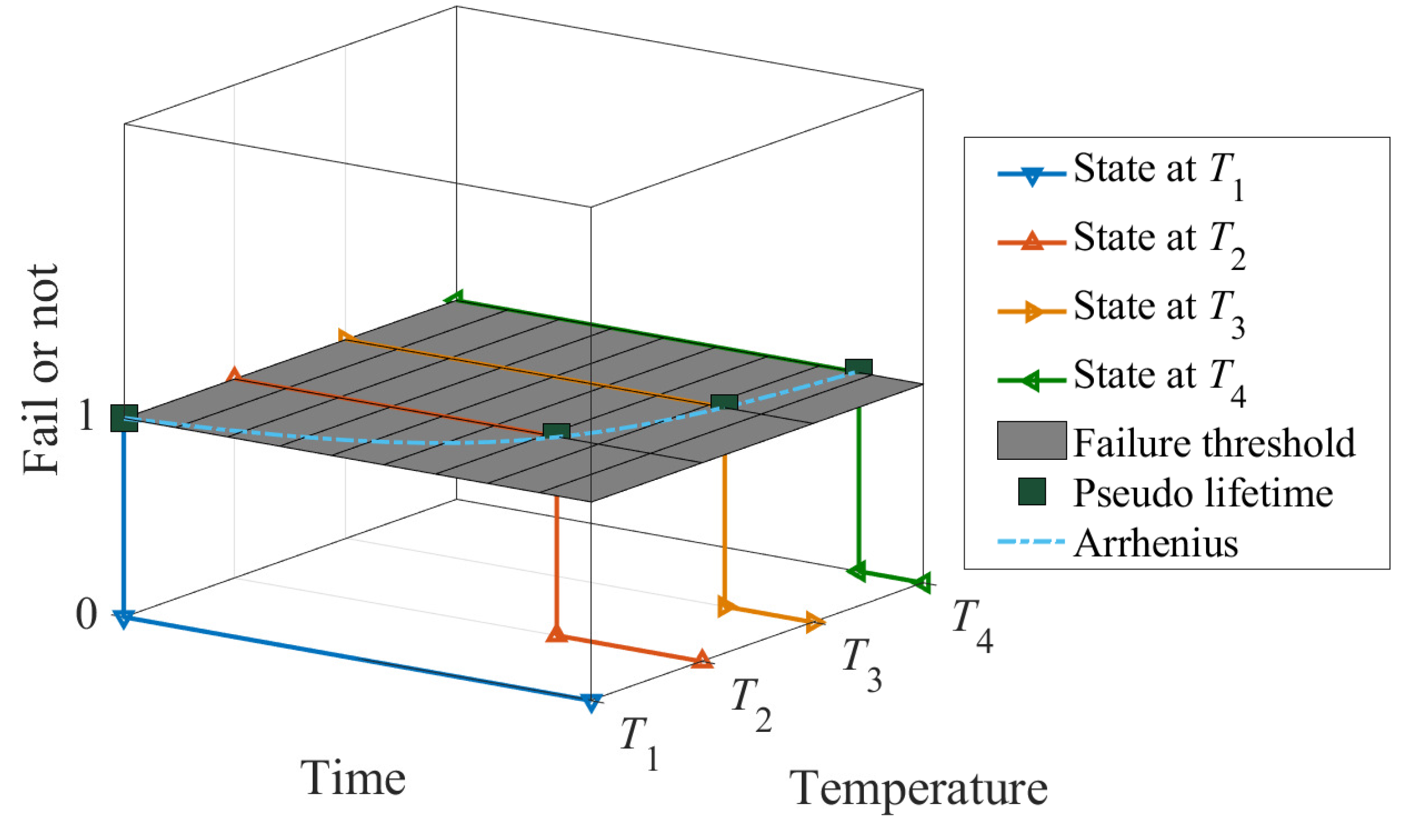
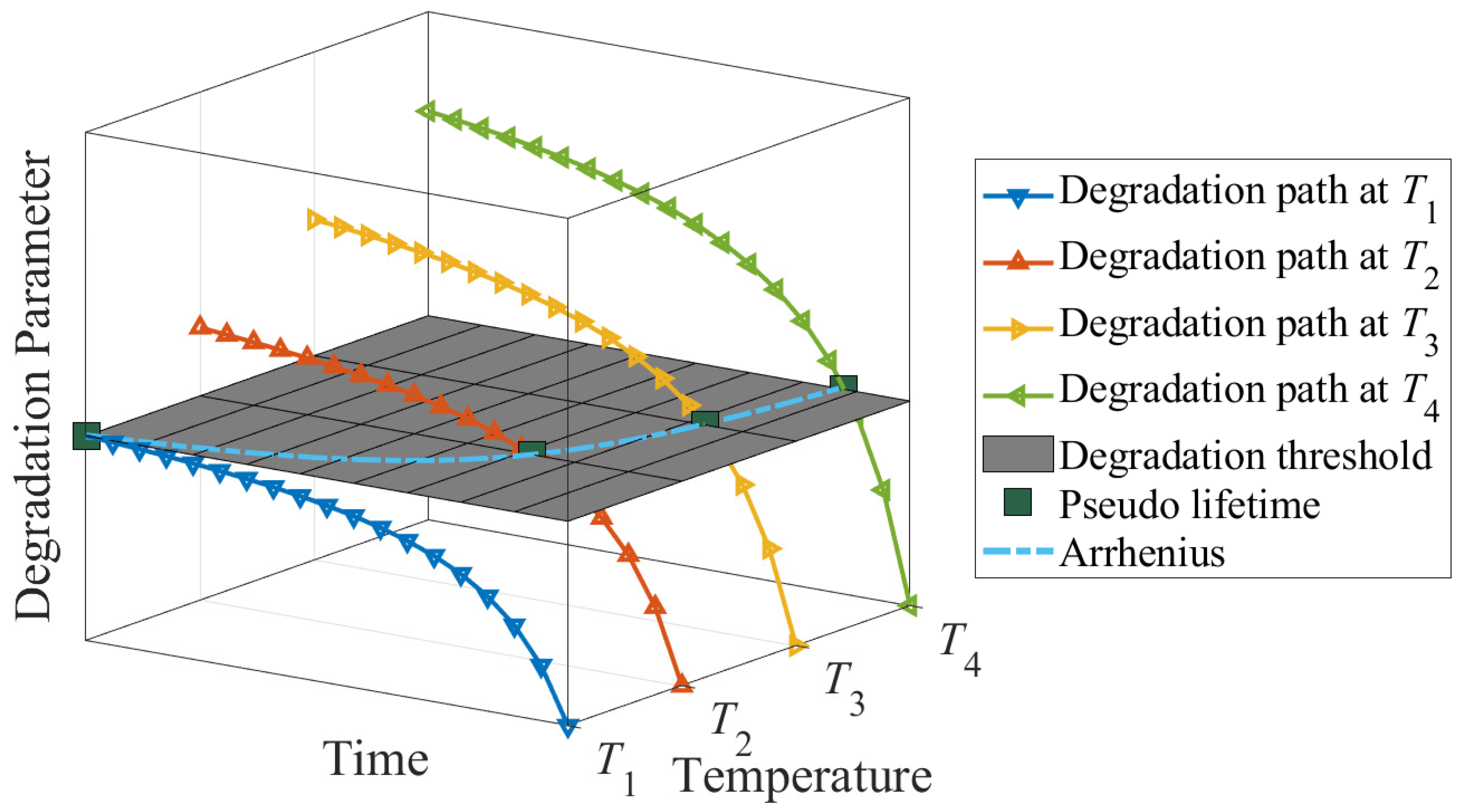
1.1. A Brief Introduction to the Accelerated Lifetime and Degradation Tests

To avoid unanticipated product failures, it is of interest to estimate a product’s lifetime, of which, the procedure can be generally described as lifetime prediction [1]. The most ideal way to acquire the lifetime of a product should be by putting the product to work under its actual operating condition, which is also referred to as the normal stress condition. However, this is exceedingly costly in terms of time, as most electronic products are designed and, therefore, expected to be useful for a decade, if not longer, and, thus, do not attract any pragmatism. To that end, it is customary to conduct lifetime prediction under abnormal stress conditions, insofar as the relationship between stress and lifetime can be drawn with some certainty. To state it differently, if the product is able to exhibit the same degradation within a shorter time period but under higher stress, such a procedure may be regarded as an accelerated test. In accelerated tests of various kinds, the most commonly applied stress is in the form of temperature. In that, the Arrhenius model is popularly used to narrate how elevated temperature, in contrast to normal operating temperature, is able to speed up degradation.
To illustrate the concept, Figure 1 shows an example of how the lifetime of an arbitrary product (i.e., spring) varies in accordance with four different temperature stress conditions, namely, T 1 , T 2 , T 3 , and T 4 . This type of accelerated test is used in situations where degradation is not measurable; thus, one can only observe the dichotomous events of “failure” and “not failure”; this is known as the accelerated lifetime test (ALT). In our example, suppose the degradation of the spring is not measurable but can only be observed through whether the spring has broken, then ALT is suitable. In ALTs, the time to failure under a particular stress condition is called the pseudo-lifetime under that stress. The correspondence between stress conditions and pseudo-lifetime can be described by the Arrhenius model, which is indicated by the dashed curve in Figure 1. The curve, as with any mathematical function, has several parameters controlling its shape, which can be estimated when multiple sets of stress conditions and pseudo-lifetimes are available. Once the curve is estimated, one may subsequently input the normal operating temperature, say T 0 , into the model, and arrive at a predicted lifetime of the product.
The accelerated degradation test (ADT) is similar to ALT. In ADTs, the degradation of the product of concern is measurable or can be represented by some intermediate but measurable quantities, known as degradation parameters. For instance, the degradation parameter of the spring could be the force. By observing how the degradation parameters change over time and under different stress conditions, one can predict the pseudo-lifetime or the time when the product needs to be replaced. Analogous to Figure 1, Figure 2 illustrates the degradation of the springs in an ADT setting. The four colored lines correspond to the so-called degradation paths under four different temperature stress conditions. From Figure 1, one can see that the product exhibits faster degradation under a higher temperature. But regardless, when the value of the degradation parameter reaches some pre-specified threshold, the product is regarded as “failed”, which indicates the need for replacement. In Figure 2, the intersections of those degradation curves with the pre-specified degradation threshold can again be described by an Arrhenius relationship. Once the curve is estimated, one may subsequently input the normal operating temperature, T 0 , into the model and arrive at a predicted lifetime of the product.

1.2. Literature Review

In degradation studies for products of various kinds, such as lithium-ion batteries [2], LED luminaries [3], capacitors [4], or rubber [5,6], the application of the Arrhenius model has proliferated in both ALTs and ADTs. However, it must be highlighted that the consistency between the degradation mechanism under abnormal stress conditions and operating conditions is the premise for ensuring the validity of ALT and ADT. Lu et al. [7] concluded that the silicone rubber conforms to the Arrhenius model in the step-stress accelerated degradation test and used it as the basis for the mechanism consistency checking. In the cold step-temperature test, Wang and Sun [8] insisted that the permanent degradation per unit time and the absolute temperature are also in the Arrhenius relationship, and the mechanism consistency checking of the servo system was completed accordingly. In [9], the Arrhenius equation was applied to establish the relationship between the product degradation rates and the thermal accelerated stress. Guo et al. [10] indicated that the resistance of thick film resistors is in an Arrhenius relationship with temperature, and this is the basis for discerning whether the failure mechanism is consistent. Chen et al. [11] proposed a criterion to check the mechanism consistency based on the gray theory, and its key point was whether E a in Arrhenius changes with temperature. In the above literature, the Arrhenius model is ubiquitously used as a default practice in many fields.
Although some have verified the assumption by out-of-sample tests (e.g., verifying the predictive ability of the Arrhenius model at some unseen temperatures that can be subjected to ALT or ADT, such as the hold-out samples), the validity of the model is only within a temperature range, and this range differs from one material/product to another. This drawback, which is called the non-Arrhenius phenomenon, has been pointed out by numerous works in the literature. For instance, Celina et al. [12] argued that the degradation of rubber does not follow the Arrhenius model, and this viewpoint has been subsequently repeated by Wang et al. [13], who concluded that the model is not suitable for rubber lifetime prediction beyond the range of 50–120 °C. Similarly, Wang et al. [14] pointed out that a single Arrhenius model is insufficient in describing the behavior of the activation energy of butadiene rubber; thus, they proposed using the summation of two Arrhenius models with differing parameters instead. Rapp et al. [15] concluded that extrapolating accelerated aging tests to lower temperatures via an Arrhenius approach, in order to predict the lifetime of the polymer, leads to critical errors. Due to the non-Arrhenius phenomenon in the rubber aging process, the Arrhenius equation is modified to extrapolate the acceleration factor at low temperatures to predict rubber properties [16,17].
Even when describing temperature characteristics of materials, Arrhenius shows difficulty. A non-Arrhenius phenomenon in the temperature characteristics shows some similarities between different materials. Macdonald [18] semi-quantitatively simulated the changing trend of activation energy in the conductivity of glassy fast-ionic materials, such as the error function shown in Figure 3. The temperature characteristics of various materials, including but not limited to the permeability of a superconductor [19], the resistivity of copper [20], critical thickness for homogeneous oxidation of rubber [21], Young’s modulus of glass [22] and ceramics [23], the decomposition of CaCO 3 [24], BaCO 3 , SrCO 3 [25], as well as the α -site occupancy of the super electronic conductor AgCrSe 2 [26], all present an “inverse-S” shape of the error function. The above facts suggest that the error function provides a generalizable shape for describing temperature characteristics across different materials.
The above non-Arrhenius phenomenon suggests that a new model is now needed to be applied to the mechanism consistency checking. As elaborated in Figure 3, the error function model (EFM) proposed in this paper resembles a different shape than what the Arrhenius model can describe. Additionally, the validity of the EFM is verified in an ADT involving a few 28-V–2-A electromagnetic relays, of which, degradation is contributed to by the stress relaxation of the spring. Two degradation models, one based on EFM and the other on the Arrhenius model, are formulated and assessed for their consistency in the failure mechanism. A criterion based on the likelihood ratio test is established to gauge the models’ performance. The EFM-based degradation model output confirms the consistent failure mechanism hypothesis, whereas the output of the Arrhenius-based model does not. The evidence presented indicates that the EFM-based model output is more compelling. In short, the main contributions of this paper can be summarized as follows:
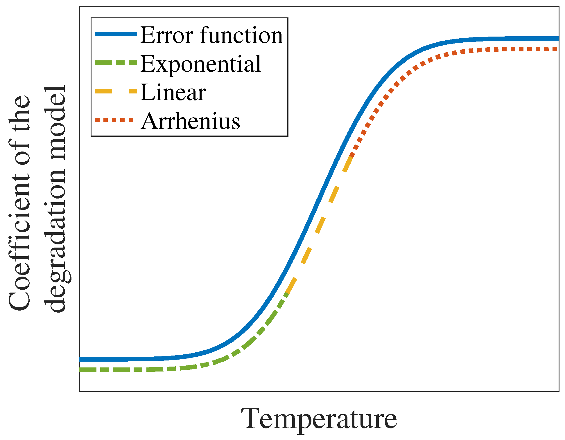
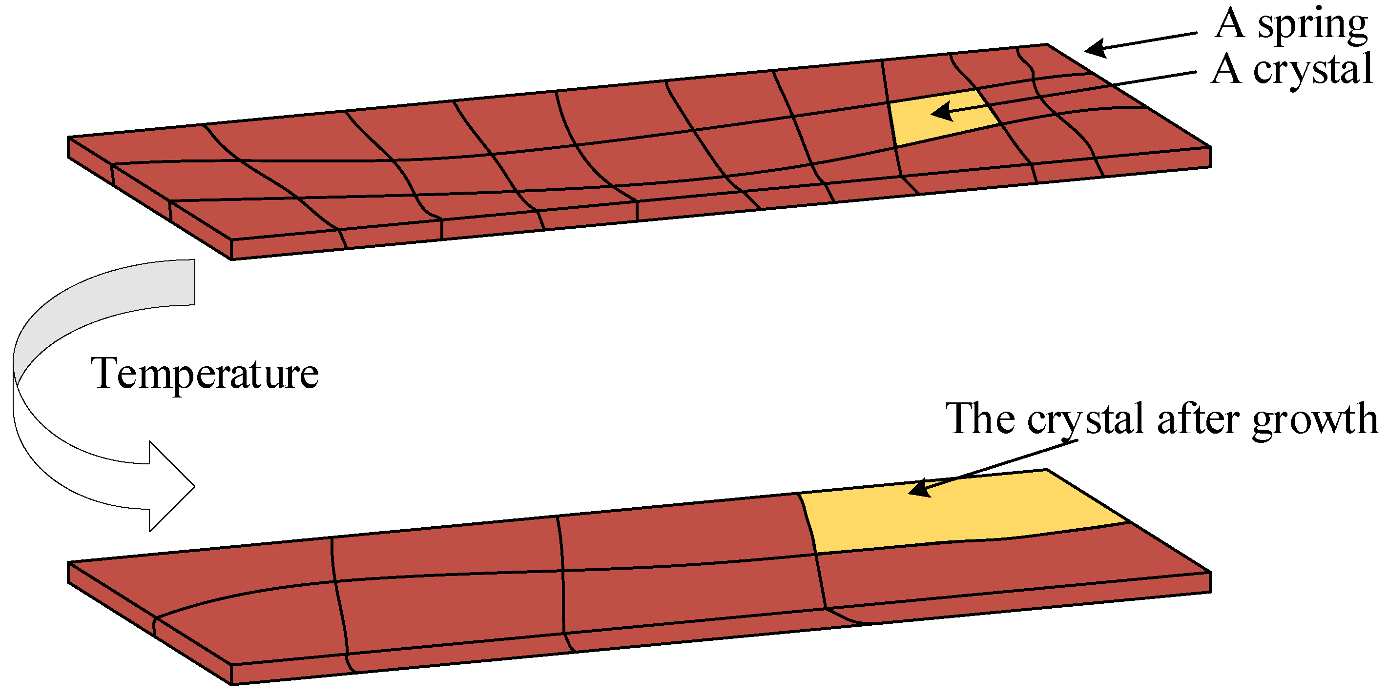
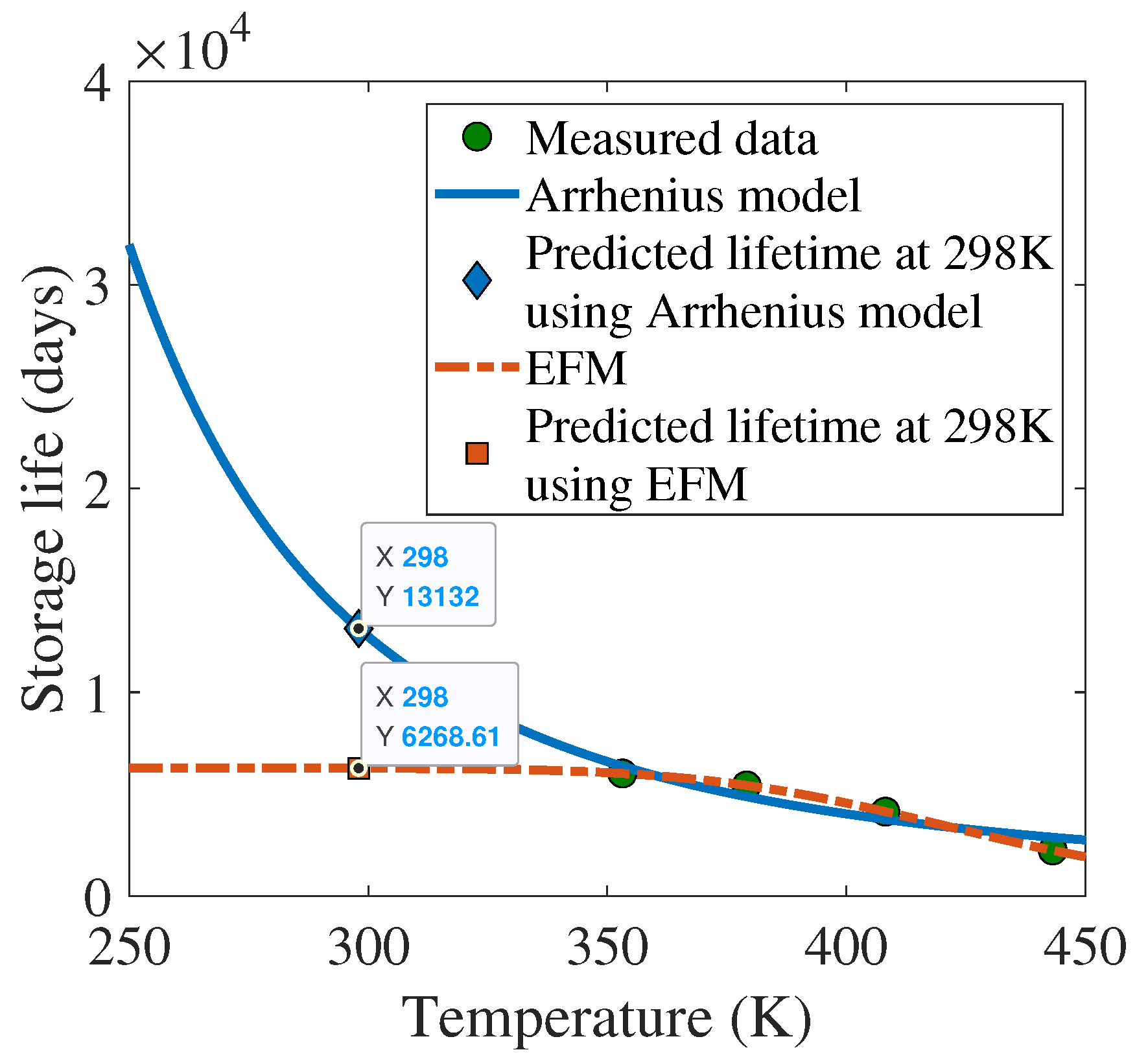
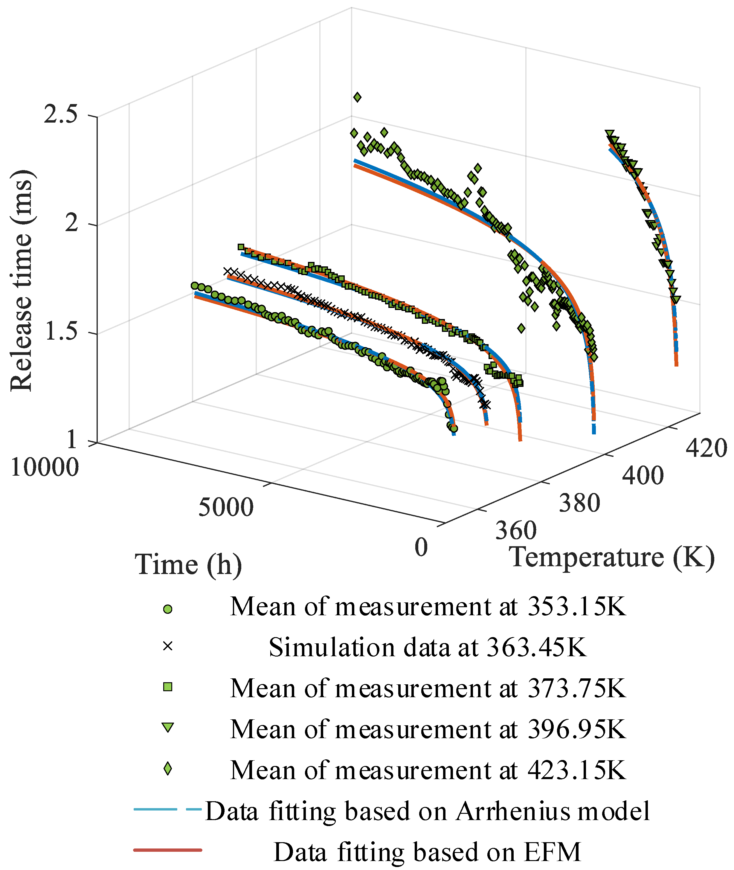
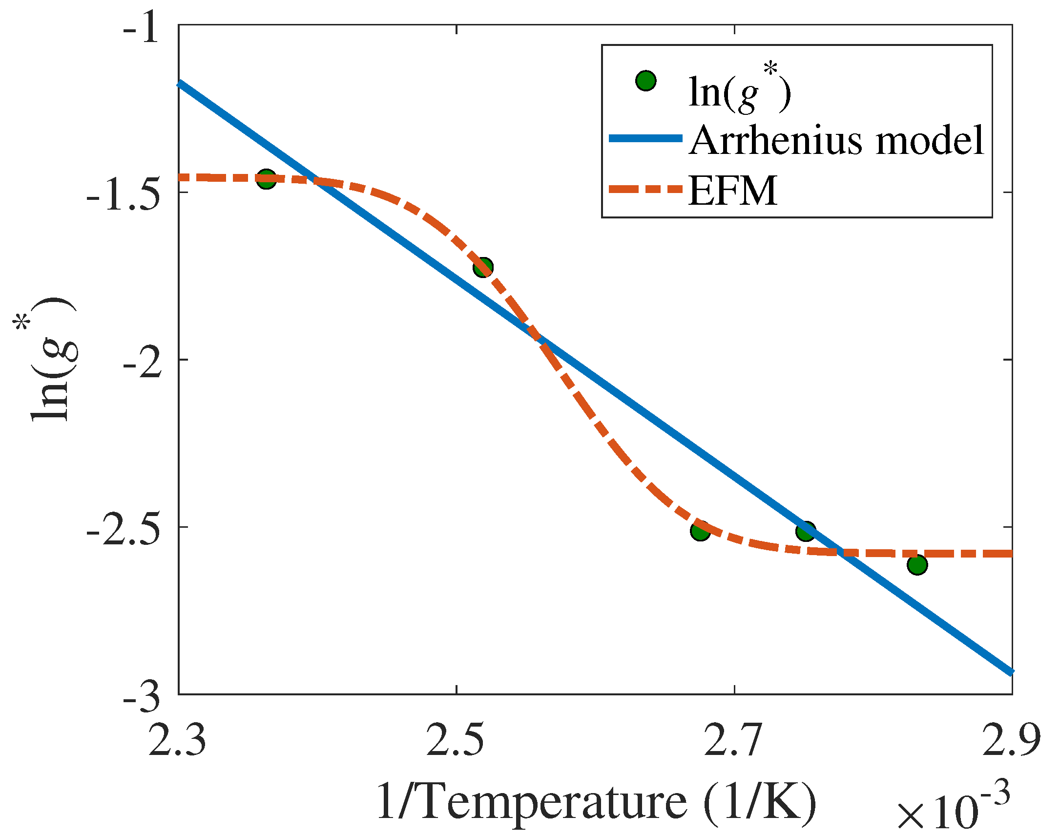
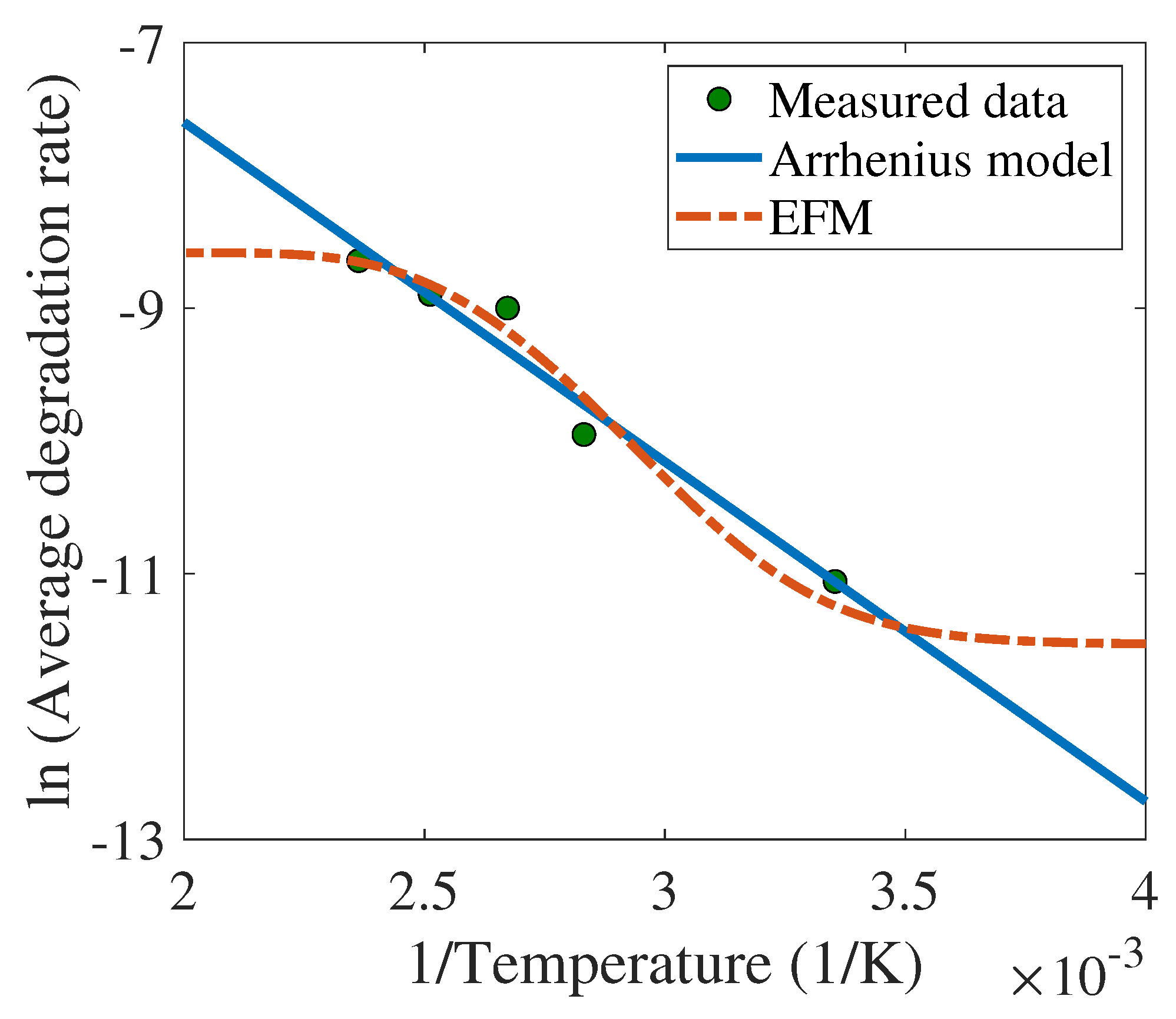
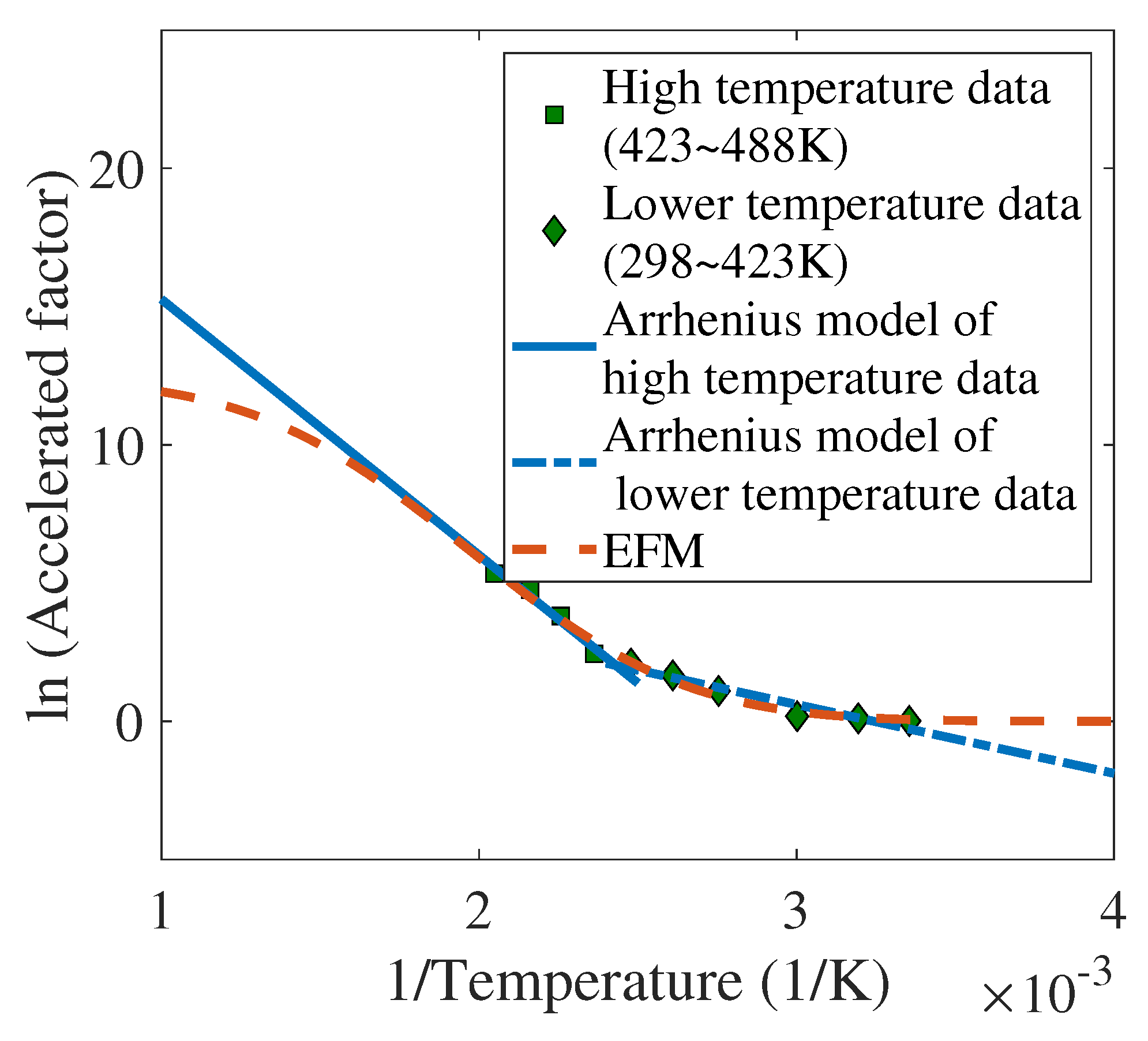
  • A non-Arrhenius model is proposed to portray the degradation behavior of electromagnetic relays under ADT. The model is based on the theory of the crystal vibration energy of the material of the spring. As compared to the conventional Arrhenius-based degradation model, EFM is able to better capture the temperature characteristics of coefficients in the degradation model (TCCDM) over a much wide temperature range (see Figure 3).
  • A procedure for degradation mechanism consistency checking is devised. The procedure leverages the statistical hypothesis (i.e., the χ 2 test), and checks whether the parameter characterizing the degradation mechanism changes or not over temperature. Analytic expressions of the partial derivatives to the likelihood function are derived, and the Bayesian information criterion is employed to compare EFM- and Arrhenius-based degradation models.
  • The proposed model can be used to explain the degradation of a wide range of materials and components, such as the capacitor or rubber.

2. Mathematical Description of the Arrhenius Model

Since the validity of applying the Arrhenius model is fundamental to precise lifetime prediction, it is of interest to take a closer look at the origin and development of the model. The Arrhenius model was originally proposed to describe the relationship between temperature and the chemical reaction rate. The model is established on a large number of chemical experiments, from which the following equation obtains:
κ = A exp E a R T ,
where κ is the temperature characteristic of the chemical reaction rate, A is a constant that needs to be estimated, E a is the experimental activation energy, R = 8.31 m 2 · kg·s 2 · K 1 · mol 1 is the molar gas constant, and T is the thermodynamic temperature in Kelvin. The function form of Equation (1) is shown in Figure 3 as the red dotted line, alongside some other functions, which will be explained below. The transfer of the application of the Arrhenius model, from the chemical reaction rate (the resultant per unit time in chemical reactions) to the degradation rate, can be traced back to 1985, when Campbell [27] used it to predict the lifetime of polyimide wire insulation in an ALT. Campbell’s procedure can be described by the following equation:
L = ϑ end ϑ 0 κ = ϑ end ϑ 0 A exp E a R T = ϑ end ϑ 0 A · exp E a R T ,
in which L is the lifetime under the corresponding stress conditions, ϑ end is the degradation parameter value when the product fails, ϑ 0 is the initial value of the degradation parameter. Equation (2) can be abbreviated as follows:
ln L = A * + B * T ,
where A * = ln ( ϑ end ϑ 0 ) / A , B * = E a / R . Equation (3) omits the estimation of non-essential parameters for lifetime prediction and is, therefore, also used more often. Recall in ALT that the degradation parameter ( ϑ end and ϑ 0 in this case) and the degradation path are not measurable and, therefore, are often perceived and assumed to be two-state. When different LT pairs are obtained experimentally, one can use the Arrhenius model to extrapolate L under arbitrary T. In other words and from Equation (2), L is only a function of temperature T, but not a function of time.
When this situation is extended to ADT, as shown in Figure 2, the degradation of ϑ 0 toward ϑ end is measurable, and more often than not, nonlinear. ϑ end is the pre-specified threshold, which is set by the investigators and domain experts. ADT is completed when the degradation path reaches ϑ end . It can be seen that the degradation paths under different stress conditions intersect with the failure threshold ϑ end at different time instances, which can be taken as the pseudo-lifetime under the corresponding stress condition. As introduced earlier, the mapping between the pseudo-lifetime and temperature is assumed to obey the Arrhenius model. The degradation model specifies the shape of the degradation path, while the degree of degradation is determined by the coefficient of the degradation model, which is considered to be the numerical representation of the degradation rate in the degradation model. Taking the stress relaxation model of the spring as an example, where stress relaxation is the degradation parameter of concern, Li [28] shows that the expression of stress relaxation is as follows:
ρ ( t , T ) = d ( T ) · ln t + e ,
where ρ is the force of the spring over time at some specific temperature T; t is the time; d and e are the coefficients of the stress relaxation model, and d is the coefficient of the degradation model in ADT and varies only with temperature rather than time. The mapping between d and temperature is also empirically considered to obey the Arrhenius model. In other words, if d at a certain temperature does not obey the Arrhenius model, it means that the degradation mechanism at this temperature is inconsistent with others, and the degradation path at this temperature should be discarded.
The original application of the Arrhenius model (chemical reaction rate) can be thought of as the temperature characteristics of the resultant per unit time in chemical reactions, evolving into the mapping between coefficients of the degradation model and temperature. In the ADT of the springs, the force of the spring corresponds to the resultant in a chemical reaction. The logical premises of these applications can be collected under two heads:
  • The temperature characteristics of degradation parameters (TCDPs) (e.g., the force of the spring over temperature) align with the shape that the Arrhenius model prescribes.
  • The temperature characteristics of coefficients in the degradation model (TCCDM) (e.g., d only changes with temperature) align with the shape of TCDP.
Following the same logic, it may be more adequate to use some other models that can be derived from TCDP, insofar as they fit the experimental outcome better, as a replacement for the Arrhenius model. This is quite necessary because the degradation behaviors of the springs, rubber, and capacitors, among other subjects under ADTs, do not always align with those observed in chemical reactions. Practically, the TCDP of the product under an ADT can be measured in just one day, which is insignificant when compared to the time required to conduct the ADT, which can take six months to a year.

3. Theory of the EFM

In view of the above discussion on the potential deficiency of the Arrhenius model, this section proposes a new model in theory for describing the TCDP of the spring, and in turn compares it with the Arrhenius model in terms of the sum of squares error using the LT pairs, which are associated with the stress relaxation of springs.

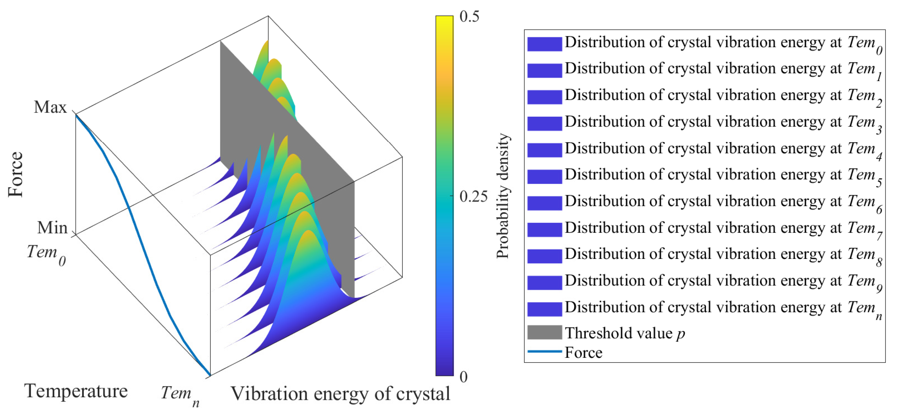
3.1. Temperature Characteristics Based on Crystal Vibration Energy

The atoms combine through bonding electrons to form a large molecule, which is called a crystal in statistical mechanics, as illustrated in Figure 4. The thermal motion of crystals can only be manifested in the form of vibrations, and the associated vibration energy is variable. As the temperature rises, the average vibration amplitude of crystals increases correspondingly. Moreover, the average vibration energy of crystals is proportional to the temperature [29]:
ζ ¯ = 1 2 h · v + k B · T ,
where ζ ¯ is the average vibration energy of crystals, h is the Planck constant, v is the quantum frequency, which can be considered as a constant, and k B is the Boltzmann constant.
Next, the connection between micro and macro nature is established upon an assumption: the macro performance of the object (e.g., the force of the metal spring) is linear to the vibration energy of crystals that are greater than threshold p:
F ( T ) = a · P ( ζ ω > p ) + b ,
where F ( T ) is the force of the spring under temperature T; ζ ω is the vibration energy of the w th crystal; a and b are constants; and P ( ζ ω > p ) denotes the probability that ζ ω > p . Furthermore, the distribution of crystal vibration energy is assumed to follow a normal distribution:
ζ ω N ζ ¯ , s 2 ,
where s is the standard deviation of the distribution of crystal vibration energy. Under the normality assumption, Equation (6) can be rewritten into:
F ( T ) = a · p 1 s 2 π exp ( z ζ ¯ ) 2 2 s 2 d z + b ,
where z is an integration variable. For the moment, s is viewed as a constant.
Equation (8) can be transformed:
F ( T ) = a * · 2 π p * c * T exp ς 2 d ς + b ,
where
ς = z ζ ¯ 2 s ,
a * = a 2 ,
p * = p 1 2 h · v 2 s ,
c * = k B 2 s .
Because a, b, h, p, v, k B , s are constants, their transformed representations a * , p * , c * are also constants. Through this transformation, F ( T ) is now expressed in the standard form of the EFM, as shown by the solid line in Figure 5. In other words, as long as the EFM resembles the measured temperature characteristics of the force of the spring, the above theory is to be regarded as valid. On this point, a test platform is built (see Figure 6). One may observe from Figure 7 that the fitted EFM is able to effectively explain the measured data points. Insofar as the current example can demonstrate, EFM is suitable for describing temperature characteristics of the spring (i.e., the TCDP) and is better than the Arrhenius model, which is incapable of prescribing an “inverse-S” shape curve.

3.2. Comparison of the Arrhenius Model and EFM

In this subsection, we employ an example to further demonstrate the difference between the Arrhenius model and EFM. The experimental data of concern come from [30], in which the LT pairs of electromagnetic relays were measured. The degradation of electromagnetic relays is mainly contributed to by the stress relaxation of the spring [30,31]. Similar to how the Arrhenius model works in ALT, EFM was used to predict the lifetime of electromagnetic relays. As shown in Figure 8, there is a considerable deviation in the predicted lifetime at 298 K (or 25 °C) using the two models. Since it is not practical in terms of time to validate the true degradation at this temperature, we turn to another perspective and focus on the goodness of fitting. Visually, it is evident that the curvature of the Arrhenius model is opposite to that of data points. In terms of quantitative assessment, it is found that the sum of squares error (SSE) of the Arrhenius model is 98,985.29 and that of EFM is only 2.31. Clearly, the lifetime predicted using EFM is more precise than that using the Arrhenius model, for the electromagnetic relay in question.

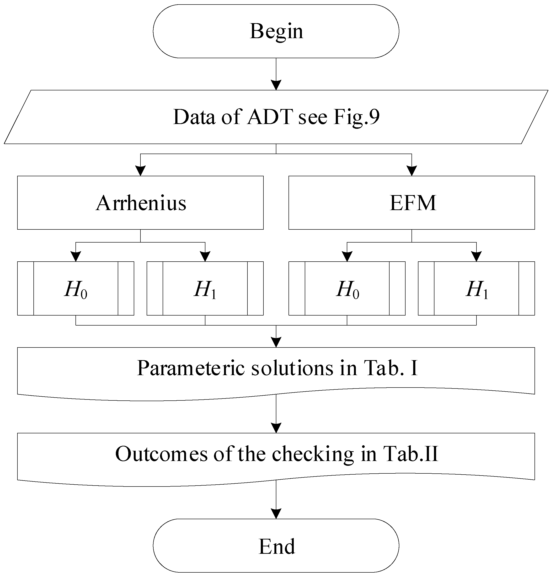
4. Procedure for Mechanism Consistency Checking

For a more detailed investigation of the difference in TCCDM between the Arrhenius model and EFM, the consistency of the degradation mechanism for electromagnetic relays under several temperature stress conditions is checked. However, before the mechanism consistency checking, two things need to be done:
  • Establish a degradation model;
  • Define a criterion for mechanism consistency checking.

4.1. Degradation Model

To describe the samples in the accelerated tests, a set of indexes will first be defined. We use i = 1 , , m to index the m temperature values, under which the degradation measurements are conducted. Next, we devise j to index the test samples (i.e., relays) under each temperature, i.e., j = 1 , , n i , where n i is the number of test samples under temperature T i . Finally, we use k to index the number of measurements, in that, k = 1 , , l i , where l i is the number of measurements made under temperature T i .
Suppose a measurement of the release time of the relay is denoted as y, the modeled counterpart is D t i j k , T i , which is a function of T i and t i j k , and the remaining difference (namely, the error) is denoted as ϵ i j k , then, the degradation model can be written as follows:
y i j k = D t i j k , T i + ϵ i j k .
It should be noted that D ( · ) is also a function of the stress relaxation model ρ and the accelerated model k ( T i ) or F ( T i ) , see below. The error term ϵ i j k is assumed to be heterogeneous and follows a normal distribution with mean zero and variance σ 2 :
ϵ i j k N 0 , σ 2 ,
which explains both the equipment’s measurement uncertainty and the warm box’s non-uniformity.
The release time is the degradation parameter of the electromagnetic relay, where degradation is mainly caused by the stress relaxation of the spring. In [28], it is emphasized that the relationship between the release time and the force of the spring is approximately linear,
D t i j k , T i = g · ρ + θ ,
where g and θ are constants. By substituting ρ with Equation (4), the above equation becomes:
D t i j k , T i = g · ρ + θ = g · d · ln t + e + θ = g * · ln t + θ * ,
where g * = d · g and θ * = e · g + θ are the coefficients in the degradation model of the electromagnetic relay under ADT; g * is a form of the degradation rate, similar to d ( T ) in Equation (4). In the case of applying the Arrhenius model, D ( · ) is expressed as follows:
D t i j k , κ T i = A exp E a R T i · ln t i j k + θ i j * ,
where D t i j k , κ T i is a function of the stress relaxation model ρ and the accelerated model k ( T i ) , θ * i j is the coefficient of the j t h sample under i t h test temperature. In the case of applying EFM, D ( · ) is modified as follows:
D t i j k , F T i = a * · 2 π p * c * T i exp ς 2 d ς + b · ln t i j k + θ i j * ,
where D t i j k , F T i is a function of the stress relaxation model ρ and the accelerated model F ( T i ) . It should be highlighted that during the numerical calculation of EFM, the power series expansion can be used to reduce the calculation burden. The expansion is as follows:
F T i = 2 a * π p * c * T i exp ς 2 d ς + b = 2 a * π π 2 ϱ = 0 ( 1 ) ϱ p * c * T i 2 ϱ + 1 ϱ ! 2 ϱ + 1 + b 2 a * π π 2 ϱ = 0 max ( ϱ ) ( 1 ) ϱ p * c * T i 2 ϱ + 1 ϱ ! 2 ϱ + 1 + b
where max ( ϱ ) is empirically set to 20.

4.2. Criteria for Mechanism Consistency Checking

The term“mechanism consistency checking” refers to whether the degradation mechanism is consistent under each acceleration stress condition; this can be framed as a well-defined hypothesis testing problem. More specifically, the null hypothesis ( H 0 ) states that the degradation mechanism is consistent under each acceleration stress, whereas the alternative hypothesis ( H 1 ) suggests otherwise, i.e., the degradation mechanisms are not the same across different acceleration stress conditions. Since the degradation mechanism is related to the degradation model parameter, one may consider the likelihood ratio test in this scenario. The likelihood ratio test is a useful tool to determine whether the estimated parameter (after certain additional restrictions are applied, e.g., the range in which the parameter assumes value) is consistent with the original parameter.
In the present case, H 0 corresponds to the case with the fixed model parameter, whereas H 1 corresponds to the case where the model parameter varies across stress conditions. Assuming that the parameter restriction is valid, it would only imply a minor deviation to the maximum value of the likelihood function, as expressed below:
Λ = 2 ln L 0 Θ ^ 0 MLE ln L 1 Θ ^ 1 MLE ,
Λ χ 2 ξ 0 ξ 1 ,
where L 0 Θ ^ 0 MLE is a log-likelihood function evaluated at Θ ^ 0 MLE , which is the maximum likelihood estimate under H 0 ; L 1 Θ ^ 1 MLE is the log-likelihood function evaluated at Θ ^ 1 MLE , which is the maximum likelihood estimate under H 1 ; the test statistic Λ obeys the χ 2 distribution with the degree of freedom | ξ 0 ξ 1 | [7]; ξ 0 and ξ 1 are the numbers of the parameters under H 0 and H 1 , respectively. At a particular significance level α , the following can be established:
P Λ > χ α 2 ξ 0 ξ 1 = α ,
where χ α 2 ξ 0 ξ 1 is the critical value at that significance level, which can be obtained by looking up the table of the χ 2 distribution. If Λ χ α 2 ξ 0 ξ 1 , H 0 is retained; if Λ > χ α 2 ξ 0 ξ 1 , H 0 is rejected. Here, α is taken as 0.05 without loss of generality.

4.3. Parameter Estimation

As per the assumption presented in Equation (15), it is possible to write the log-likelihood function ln L , up to an additive constant, as follows:
ln L = i = 1 m j = 1 n i k = 1 l i y i j k D t i j k , T i 2 2 σ 2 ln σ .
In the context of the Arrhenius model, H 0 represents the fact that the same failure activation energy E a / R applies across all temperature conditions. The log-likelihood function L 0 has the parameter Θ 0 = { A , E a , θ i j * , σ } , with partial derivatives:
ln L 0 ( Θ 0 ) A = i = 1 m j = 1 n i k = 1 l i 1 2 σ 2 · y i j k D t i j k , T i 2 A = i = 1 m j = 1 n i k = 1 l i y i j k D t i j k , T i σ 2 · D t i j k , T i A = i = 1 m j = 1 n i k = 1 l i y i j k D t i j k , T i σ 2 · exp E a R T i · ln t i j k ,
ln L 0 ( Θ 0 ) E a = i = 1 m j = 1 n i k = 1 l i 1 2 σ 2 · y i j k D t i j k , T i 2 E a = i = 1 m j = 1 n i k = 1 l i y i j k D t i j k , T i σ 2 · D t i j k , T i E a = i = 1 m j = 1 n i k = 1 l i y i j k D t i j k , T i σ 2 · A R T i · exp E a R T i · ln t i j k ,
ln L 0 ( Θ 0 ) θ i j * = k = 1 l i 1 2 σ 2 · y i j k D t i j k , T i 2 θ i j * = k = 1 l i y i j k D t i j k , T i σ 2 · D t i j k , T i θ i j * = k = 1 l i y i j k D t i j k , T i σ 2 ,
ln L 0 ( Θ 0 ) σ = i = 1 m j = 1 n i k = 1 l i 1 σ 3 · y i j k D t i j k , T i 2 σ 2 .
H 1 means that the value of E a / R in Equation (18) is not a fixed parameter, but assumes different values for different temperature conditions. The log-likelihood function L 1 has the parameter Θ 1 = { A , E a , i , θ i j * , σ } , in that, a unique value of g i * (the output of A, E a , i using Equation (1), i data points, including the i + 1 parameters to be solved) is obtained at each temperature point. It should be noted that the number of parameters in the log-likelihood function needs to be reduced, otherwise, one has undetermined systems of the equation during parameter estimation. With the new parameter Θ 1 * = { κ i , θ i j * , σ } equaling Θ 1 , the partial derivatives of the log-likelihood function are as follows:
ln L 1 ( Θ 1 * ) κ i = j = 1 n i k = 1 l i 1 2 σ 2 · y i j k D t i j k , T i 2 κ i = j = 1 n i k = 1 l i y i j k D t i j k , T i σ 2 · D t i j k , T i κ i = j = 1 n i k = 1 l i y i j k D t i j k , T i σ 2 · ln t i j k ,
ln L 1 ( Θ 1 * ) θ i j * = k = 1 l i 1 2 σ 2 · y i j k D t i j k , T i 2 θ i j * = k = 1 l i y i j k D t i j k , T i σ 2 · D t i j k , T i θ i j * = k = 1 l i y i j k D t i j k , T i σ 2 ,
ln L 1 ( Θ 1 * ) σ = i = 1 m j = 1 n i k = 1 l i 1 σ 3 y i j k D t i j k , T i 2 σ 2 .
In the context of EFM, H 0 implies that the threshold value p * in Equation (19) remains constant at each temperature condition. The log-likelihood function has the parameter Θ 0 = { a * , p * , c * , b , θ i j * , σ } . Its partial derivatives concerning each parameter are as follows:
ln L 0 ( Θ 0 ) a * = i = 1 m j = 1 n i k = 1 l i 1 2 σ 2 · y i j k D t i j k , T i 2 a * = i = 1 m j = 1 n i k = 1 l i y i j k D t i j k , T i σ 2 · D t i j k , T i a * = i = 1 m j = 1 n i k = 1 l i y i j k D t i j k , T i σ 2 · 2 π p * c * T i exp ς 2 d ς · ln t i j k ,
ln L 0 ( Θ 0 ) p * = i = 1 m j = 1 n i k = 1 l i 1 2 σ 2 · y i j k D t i j k , T i 2 p * = i = 1 m j = 1 n i k = 1 l i y i j k D t i j k , T i σ 2 · D t i j k , T i p * = i = 1 m j = 1 n i k = 1 l i y i j k D t i j k , T i σ 2 · a * · 2 π · exp ( p * c * T i ) 2 · ln t i j k ,
ln L 0 ( Θ 0 ) c * = i = 1 m j = 1 n i k = 1 l i 1 2 σ 2 · y i j k D t i j k , T i 2 c * = i = 1 m j = 1 n i k = 1 l i y i j k D t i j k , T i σ 2 · D t i j k , T i c * = i = 1 m j = 1 n i k = 1 l i y i j k D t i j k , T i σ 2 · a * · 2 π · exp ( p * c * T i ) 2 · T i · ln t i j k ,
ln L 0 ( Θ 0 ) b = i = 1 m j = 1 n i k = 1 l i 1 2 σ 2 · y i j k D t i j k , T i 2 b = i = 1 m j = 1 n i k = 1 l i y i j k D t i j k , T i σ 2 · D t i j k , T i b = i = 1 m j = 1 n i k = 1 l i y i j k D t i j k , T i σ 2 · ln t i j k ,
ln L 0 ( Θ 0 ) θ i j * = k = 1 l i 1 2 σ 2 · y i j k D t i j k , T i 2 θ i j * = k = 1 l i y i j k D t i j k , T i σ 2 · D t i j k , T i θ i j * = k = 1 l i y i j k D t i j k , T i σ 2 ,
ln L 0 ( Θ 0 ) σ = i = 1 m j = 1 n i k = 1 l i 1 σ 3 y i j k D t i j k , T i 2 σ 2 .
In Equations (12) and (13), the excessive temperature will change s and, thus, change p * c * T . Following that, for the EFM under H 1 , the log-likelihood function has the parameter Θ 1 = { a * , p i * , c i * , b , θ i j * , σ } . A unique value of g i * (the output of a * , p i * , c i * , b using Equation (9), i data points, including 2 · i + 2 parameters to be solved) is obtained at each temperature point. Similar to the case where the Arrhenius model was used, parameter reduction is required. With the new parameter Θ 1 * = { F i , θ i j * , σ } equaling Θ 1 , the partial derivatives of the log-likelihood function are as follows:
ln L 1 ( Θ 1 * ) F i = j = 1 n i k = 1 l i 1 2 σ 2 · y i j k D t i j k , T i 2 F i = j = 1 n i k = 1 l i y i j k D t i j k , T i σ 2 · D t i j k , T i F i = j = 1 n i k = 1 l i y i j k D t i j k , T i σ 2 · ln t i j k ,
ln L 1 ( Θ 1 * ) θ i j * = k = 1 l i 1 2 σ 2 · y i j k D t i j k , T i 2 θ i j * = k = 1 l i y i j k D t i j k , T i σ 2 · D t i j k , T i θ i j * = k = 1 l i y i j k D t i j k , T i σ 2 ,
ln L 1 ( Θ 1 * ) σ = i = 1 m j = 1 n i k = 1 l i 1 σ 3 y i j k D t i j k , T i 2 σ 2 .
When estimating the parameters, the maximum log-likelihood value is obtained by finding the values that satisfy the condition where the partial derivatives of the log-likelihood functions under H 0 or H 1 are equal to 0. It is noteworthy that L 1 , with both the Arrhenius model and EFM, share the same solution, although their parameterizations are different.

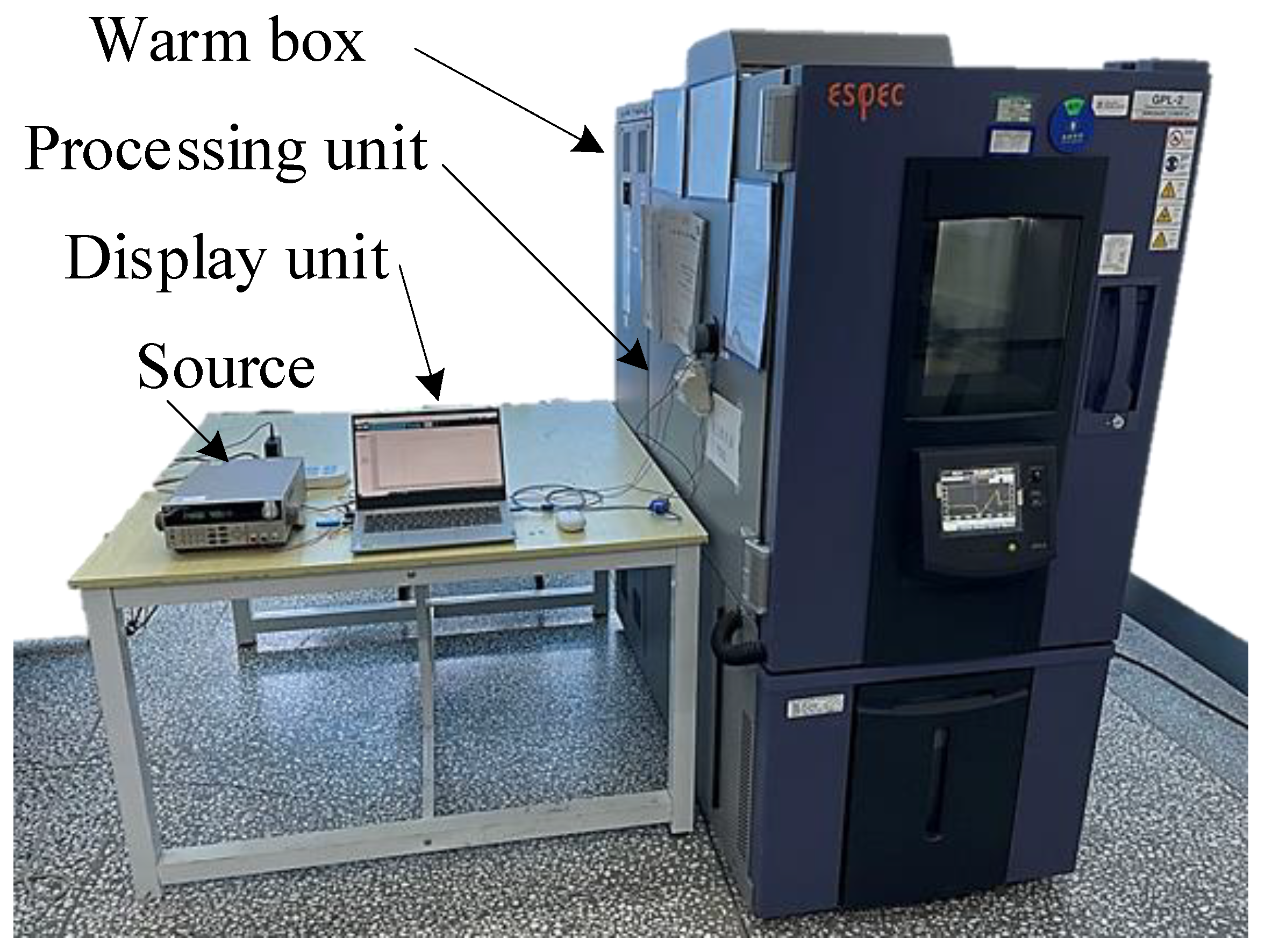
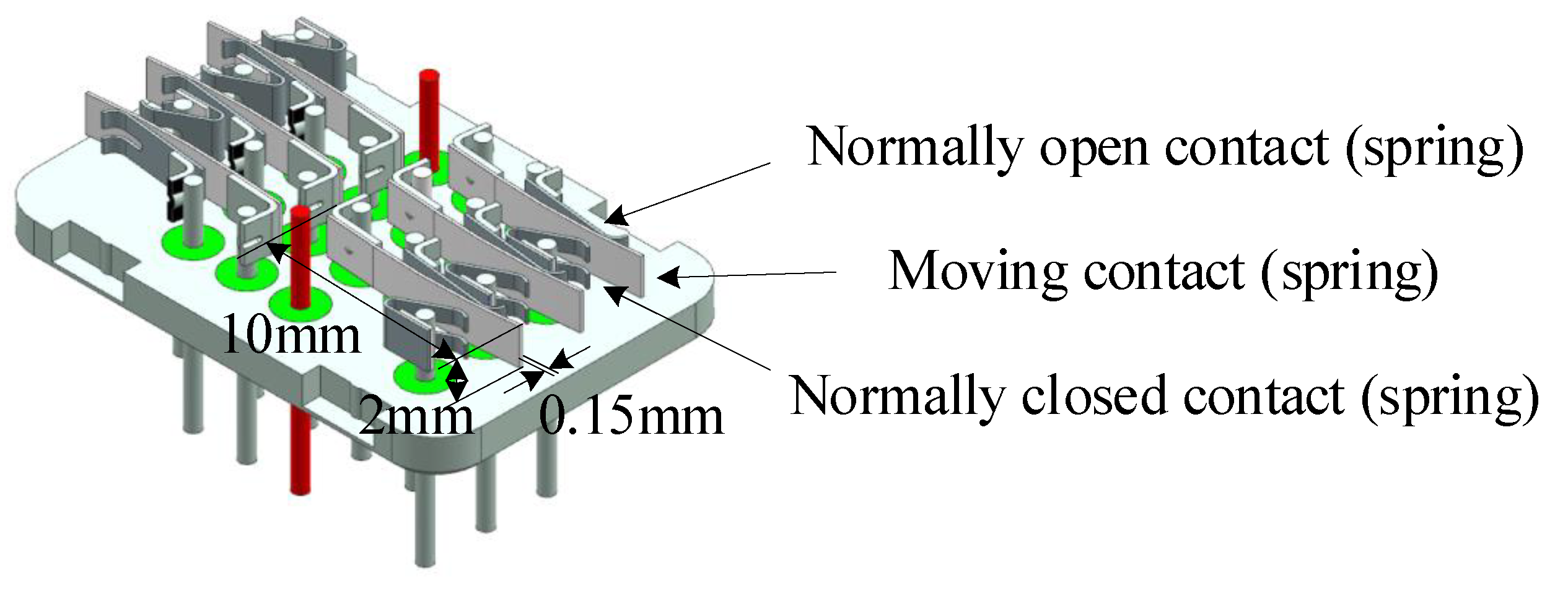
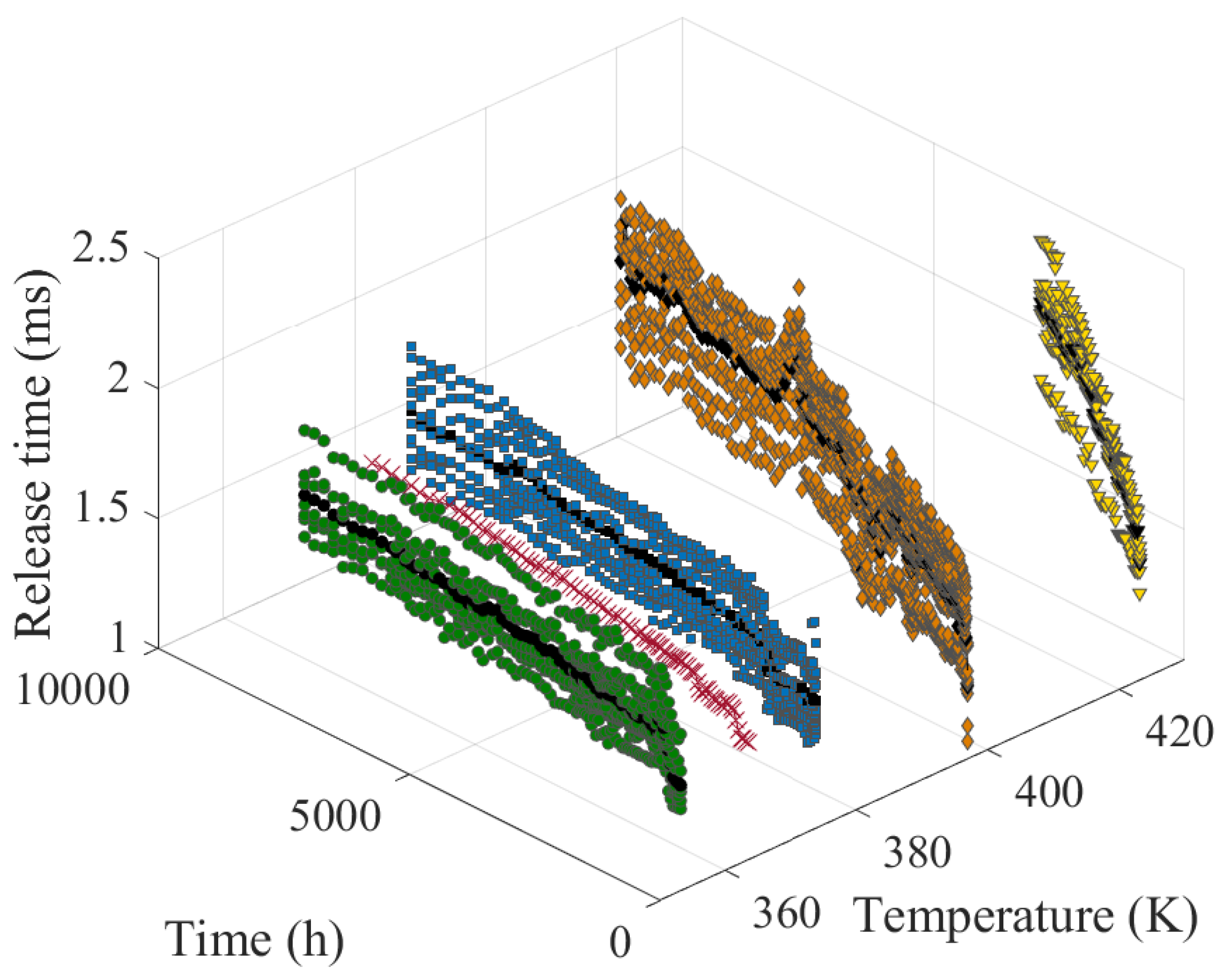
5. Case Study on the Degradation of Electromagnetic Relays

The proposed EFM alongside its mechanism consistency checking procedure may be applied to a wide range of applications where ADT is involved. In this section, two case studies are presented in order to empirically validate the proposal. Both case studies consider electromagnetic relays as the test subjects. However, what is different is the choice of the degradation parameter selected to quantify the degradation. In the first case study, the stress relaxation of the spring inside the relay is taken as the degradation parameter, whereas in the second one, the loss of the spring force is taken as the degradation parameter.

5.1. Stress Relaxation as the Degradation Parameter

In this military electromagnetic relay, silver–magnesium–nickel alloy serves as both the spring and the contact, as shown in Figure 9. The contact structure of the electromagnetic relay is composed of normally open springs, moving springs, and normally closed springs made of silver–magnesium–nickel alloy. Among them, the stress relaxation of the moving springs is the most serious. As illustrated in Figure 10, the accelerated degradation test is conducted for electromagnetic relays, with the stress relaxation of the spring being the degradation parameter, under four temperature conditions, namely, 353.15 K, 373.75 K, 396.95 K, and 423.15 K, with 7, 10, 10, and 7 relays, respectively.
Stress relaxation is thought to be the main cause of relay degradation, which is characterized by an increase in relaxation time. The corresponding testing durations are 7488 h, 8040 h, 6912 h, and 1968 h, with a total of 91, 93, 139, and 41 measurements conducted at each temperature. In order to simplify the case study, in terms of reducing the number of parameters to be estimated, data from multiple test samples under each temperature condition are aggregated. Consequently, indexes j in y, ϵ , θ * can be saved, which implies that the data under each temperature condition are lumped as a single test sample.
Recall that the hypothesis testing described in Section 4.2 requires one to compute Λ . In the case of EFM, it is noted that Θ 0 = { a * , p * , c * , b , θ 1 * , , θ 4 * , σ } , which implies ξ 0 = 9 , and on the other hand, Θ 1 = { F 1 , , F 4 , θ 1 * , , θ 4 * , σ } , which implies ξ 1 = 9 . This is problematic because the degree of freedom of the χ 2 distribution in Equation (22) is then zero, making it impossible to test the consistency of the failure mechanism for ADT. To circumvent this situation, one can consider synthetically generating data for an additional temperature to increase the degrees of freedom in Λ . In particular, because the data points at temperatures 353.15 K and 373.75 K possess similar visual degradation behaviors, one can interpolate between those two sets of data points at another temperature, of which, the results are marked as the red data points in Figure 10. With the additional set of “measurements”, the situation is now transformed into Θ 0 = { a * , p * , c * , b , θ 1 * , , θ 5 * , σ } , with ξ 0 = 10 , and Θ 1 = { F 1 , , F 5 , θ 1 * , , θ 5 * , σ } , with ξ 1 = 11 . The degree of freedom for the χ 2 distribution in Equation (22) is then 1, allowing to test the consistency of the failure mechanism for ADT.
Using the procedure outlined in Figure 11, the consistency of the degradation mechanism can be verified. The degradation model has two variants, namely, the one based on the Arrhenius model and that based on EFM. For each variant, there are two scenarios, which correspond to H 0 and H 1 , respectively. Table 1 tabulates the parameter estimation results of the above variants and scenarios. The fitted degradation models under each temperature condition are shown in Figure 12.
The results of the mechanism consistency checking are presented in Table 2, and the two models yield opposite conclusions regarding the hypothesis. However, since both models are essentially describing the TCCDM of electromagnetic relays, it is not possible to determine which model is better, and an additional technique is required to make such a distinction. On this point, both visual- and information-criterion-based methods are considered. In the case of the former, ln ( g * ) is plotted against the temperature, as shown in Figure 13, and one can see that the EFM is evidently closer in the form of the empirical estimates. Next, quantitatively, the Bayesian information criterion (BIC) is used, which states the following:
BIC = ln ( r ) · ι 2 ln L ^
where L ^ is the maximized value of the likelihood function of the model, ι is the number of parameters estimated by the model, and r is the sample size. When BIC is negative, the smaller its value is, the better the model is. There are 455 samples in the ADT; the EFM-based degradation model consists of 10 parameters, whereas the Arrhenius-based degradation model consists of 8 parameters. It is found that the BIC of EFM in H 0 is 1103.40 , while that of Arrhenius in H 0 is 1088.14 . As a result, it is reasonable to believe that the outcome based on EFM is more accurate, as concluded from Figure 8. In general, the degradation rate typically increases with temperature until it reaches an upper limit, as specified by the Arrhenius model. However, the EFM provides additional insight by specifying a lower bound for the degradation rate at low temperatures. This has been supported by various studies in the literature [16,17].

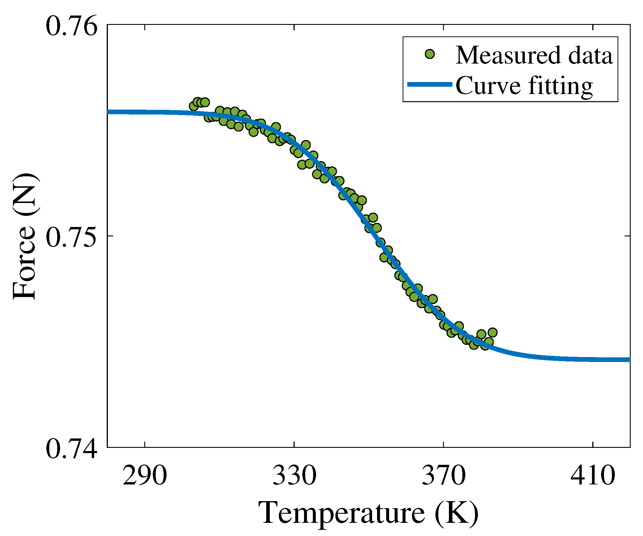
5.2. Loss of Spring Force as the Degradation Parameter

In this part of the work, we discuss the applicability of EFM with the loss of the spring force being the degradation parameter. The stress relaxation of the spring inside the electromagnetic relay, which manifests externally as an increase in relaxation time, may be subject to the loss of information during the conversion process from internal to external. To investigate this process of degradation more intuitively, we directly measure the loss of the spring force before and after the accelerated degradation test by opening the shells of relays. During the production of electromagnetic relays undergoing accelerated degradation tests, researchers measured the force of the spring ( F 0 ). After completing the accelerated degradation tests for electromagnetic relays, they opened the shells of these relays and tested the force of the spring ( F 1 ). The difference between F 0 and F 1 is referred to as force loss.
As shown in Table 3, there are five data points (i.e., five relays), among which, the relay at 298.15 K is not subjected to ADT (i.e., normal working condition), whereas the remaining four undergo ADT. The degradation rate is defined as the loss of the spring force divided by time. Under the assumption that the degradation is linear, this degradation rate can also be regarded as the TCCDM. Therefore, it can also be modeled using the Arrhenius model and EFM. Let ϵ represent the difference between the modeled data and the test data. It is assumed that the measured errors ϵ obey a normal distribution mean zero and variance σ 2 . Again, the maximum log-likelihood values ln L ^ under both the Arrhenius model and EFM are sought. According to the data, the fitting result is shown in Figure 14. The BICs are listed in Table 4, i.e., the BIC of EFM is 91.72 , while that of Arrhenius is 91.11 ; the former should be preferred. Since the loss of the spring force is not unique to springs in electromagnetic relays, but is general to all springs, the proposed EFM can no doubt be extended in such an avenue.

6. Discussion

In this section, the comparative advantages and disadvantages of the EFM over the Arrhenius model are discussed. Although the content, thus far, has focused on the ADT of electromagnetic relays, the application of EFM can be extended to other use cases, such as capacitors or rubbers, which are the most popular study subjects for ADT. More specifically, the advantage of EFM is illustrated through its wider applicable temperature range.
In the case of capacitors, it is found that the TCCDM is subject to the Arrhenius model between 339 K and 399 K (Figure 6 in [32]), is linear between 253 K and 333 K (Figure 12 in [33]), and exponential between 293 K and 353 K (Figure 7 in [34]). In other words, the Arrhenius model is only applicable within specific temperature ranges, whereas the relationship between the degradation parameter and temperature (i.e., the degradation rate) takes different shapes over different temperature ranges. However, EFM is found to be a more comprehensive model that could well describe all three shapes of degradation rates, over a much wider temperature range, as shown in Figure 3. This suggests that EFM is a better option for predicting the lifetime of capacitors under varying temperature conditions.
Similarly, in the case of rubbers, it has been concluded that the accelerated factor (a form of TCCDM that can be modeled with both EFM and the Arrhenius model) is exponential between 333 K and 423 K (Figure 7 in [35]). In another circumstance, the variation of the acceleration factor is plotted over a wider temperature range of 298 K to 488 K (Figure 4 in [36]), in that, the data of high temperatures and low temperatures are fitted by two separate Arrhenius models. This indicates that the Arrhenius model with a fixed parameter is only accurate within a limited temperature range, whereas EFM is able to model the acceleration factor without segmentation, as shown in Figure 15. Additionally, the sum of squares error of EFM is 0.42, which is lower than the 0.5 of the two Arrhenius models, indicating that EFM can provide more accurate predictions over a wider temperature range.
In comparison with the Arrhenius model, EFM offers better applicability over wider temperature ranges. However, it is more complex, thereby posing difficulties in computations. As is evident from Equation (20), its computation requires power series expansion. It follows that the higher the level of accuracy that is desired, the more intricate the calculation process could be. When applying EFM, it is imperative to maintain a balance between the level of precision and complexity of the computation.

7. Conclusions

Through the above examples of electromagnetic relays, rubbers, and capacitors, it has been shown that the Arrhenius model is not always the optimal choice in describing the TCCDM. Applying an inappropriate accelerated model can lead to the distortion of the degradation model, which further misleads any lifetime prediction made thereof. Hence, this paper proposes the EFM (recall Equation (6)), which seeks to improve upon the Arrhenius model. At relatively high temperatures, the pseudo-lifetimes (a form of the degradation rate) of electromagnetic relays do not change significantly with temperature (recall Figure 8). At relatively low temperatures, the TCCDMs (another form of the degradation rate) of electromagnetic relays (recall Figure 13) do not change significantly with temperature. These two phenomena are consistent with the shape of the proposed EFM. Moreover, the fitting results of EFM are shown to be superior to those of the Arrhenius model. In conclusion, all evidence collected in this work suggests that EFM can better describe the TCCDM than the Arrhenius model.
That being said, in the present form, the standard deviation of the Gaussian distribution (i.e., s in Equation (8)) is kept constant. However, the data in [37] reveal that the standard deviation may vary as a function of time t and temperature T, which could be viewed as a point for improvement in the current version of the EFM. In this regard, one possible direction to extend the current work is to carry out—on the electromagnetic relays—a progressive stress accelerated degradation test, where the temperature is proportional to the time. By comparing the constant loading for temperature, as in this paper, and that assuming progressive stress, the time–temperature-varying standard deviation idea, i.e., s ( t , T ) , can be verified.

Author Contributions

Methodology, R.F.; Validation, J.Y.; Resources, Y.L.; Supervision, H.L. All authors have read and agreed to the published version of the manuscript.

Funding

This research was funded by National Natural Science Foundation of China grant number NSFC 52177134, Zhejiang Provincial Natural Science Foundation of China under Grant No. LY23E070001.

Conflicts of Interest

The authors declare no conflict of interest.

References

  1. Huang, T.; Peng, B.; Coit, D.W.; Yu, Z. Degradation Modeling and Lifetime Prediction Considering Effective Shocks in a Dynamic Environment. IEEE Trans. Reliab. 2019, 68, 819–830. [Google Scholar] [CrossRef]
  2. Xu, X.; Tang, S.; Yu, C.; Xie, J.; Han, X.; Ouyang, M. Remaining useful life prediction of lithium-ion batteries based on wiener process under time-varying temperature condition. Reliab. Eng. Syst. Saf. 2021, 214, 107675. [Google Scholar] [CrossRef]
  3. Qian, C.; Fan, X.; Fan, J.; Yuan, C.; Zhang, G. An accelerated test method of luminous flux depreciation for LED luminaires and lamps. Reliab. Eng. Syst. Saf. 2016, 147, 84–92. [Google Scholar] [CrossRef]
  4. Liu, D.D. Insulation resistance degradation in Ni–BaTiO3 multilayer ceramic capacitors. IEEE Trans. Comp. Packag. Manufact. Technol. 2015, 5, 40–48. [Google Scholar] [CrossRef]
  5. Moon, B.; Jun, N.; Park, S.; Seok, C.; Hong, U. A study on the modified arrhenius equation using the oxygen permeation block model of crosslink structure. Polymers 2019, 11, 136. [Google Scholar] [CrossRef] [Green Version]
  6. Woo, C.S.; Choi, S.S.; Lee, S.B.; Kim, H.S. Useful Lifetime Prediction of Rubber Components Using Accelerated Testing. IEEE Trans. Reliab. 2010, 59, 11–17. [Google Scholar] [CrossRef]
  7. Lu, X.; Chen, X.; Wang, Y.; Tan, Y. Consistency analysis of degradation mechanism in step-stress accelerated degradation testing. Eksploat. Niezawodn. 2017, 19, 302–309. [Google Scholar] [CrossRef]
  8. Wang, X.; Sun, Q. Consistency check of degradation mechanism between natural storage and enhancement test for missile servo system. J. Syst. Eng. Electron. 2019, 30, 415–424. [Google Scholar] [CrossRef]
  9. Zhai, G.; Zheng, B.; Ye, X.; Si, S.; Zio, E. A failure mechanism consistency test method for accelerated degradation test. Qual. Reliab. Engng. Int. 2021, 37, 464–483. [Google Scholar] [CrossRef]
  10. Guo, C.; Wan, N.; Ma, W.; Zhang, Y.; Feng, S. A fast method for judging the consistency of the failure mechanism of the constant temperature stress accelerated experiment. Acta. Phys. Sin.-Ch. Ed. 2013, 62, 478–482. [Google Scholar] [CrossRef]
  11. Chen, Y.; Chen, H.; Yang, Z.; Kang, R.; Yang, Y. Consistency analysis of accelerated degradation mechanism based on gray theory. J. Syst. Eng. Electron. 2014, 25, 322–331. [Google Scholar] [CrossRef]
  12. Celina, M.; Gillen, K.; Assink, R. Accelerated aging and lifetime prediction: Review of non-Arrhenius behaviour due to two competing processes. Polym. Degrad. Stab. 2005, 90, 395–404. [Google Scholar] [CrossRef]
  13. Wang, H.; Zhao, Y.; Ma, X. Rubber lifetime prediction for ADT data considering non-arrhenius behavior. In Proceedings of the 2017 Annual Reliability and Maintainability Symposium (RAMS), Orlando, FL, USA, 23–26 January 2017; pp. 1–6. [Google Scholar] [CrossRef]
  14. Wang, Y.; Wang, W.; Liu, Q.; Cui, Z.; Wang, J. Analysis on the Non-Arrhennius life prediction method of rubber. Adv. Mater. Res. 2013, 683, 366–371. [Google Scholar] [CrossRef]
  15. Rapp, G.; Tireau, J.; Bussiere, P.O.; Chenal, J.M.; Rousset, F.; Chazeau, L.; Gardette, J.L.; Therias, S. Influence of the physical state of a polymer blend on thermal ageing. Polym. Degrad. Stab. 2019, 163, 161–173. [Google Scholar] [CrossRef]
  16. Guo, X.; Yuan, X.; Liu, G.; Hou, G.; Zhang, Z. Storage Life Prediction of Rubber Products Based on Step Stress Accelerated Aging and Intelligent Algorithm. Polymers 2023, 15, 157. [Google Scholar] [CrossRef]
  17. Guo, X.; Yuan, X.; Hou, G.; Zhang, Z.; Liu, G. Natural Aging Life Prediction of Rubber Products Using Artificial Bee Colony Algorithm to Identify Acceleration Factor. Polymers 2022, 14, 3439. [Google Scholar] [CrossRef]
  18. Macdonald, J.R. The Ngai coupling model of relaxation: Generalizations, alternatives, and their use in the analysis of non-Arrhenius conductivity in glassy, fast-ionic materials. J. Appl. Phys. 1998, 84, 812–827. [Google Scholar] [CrossRef]
  19. Zhao, L.; Liang, A.; Yuan, D.; Hu, Y.; Liu, D.; Huang, J.; He, S.; Shen, B.; Xu, Y.; Liu, X.; et al. Common electronic origin of superconductivity in (Li,Fe)OHFeSe bulk superconductor and single-layer FeSe/SrTiO3 films. Nat. Commun. 2016, 7, 10608. [Google Scholar] [CrossRef] [Green Version]
  20. Nakane, H.; Watanabe, T.; Nagata, C.; Fujiwara, S.; Yoshizawa, S. Measuring the temperature dependence of resistivity of high purity copper using a solenoid coil SRPM method. IEEE Trans. Instrum. Meas. 1992, 41, 107–110. [Google Scholar] [CrossRef]
  21. Celina, M.; Graham, A.C.; Gillen, K.T.; Assink, R.A.; Minier, L.M. Thermal Degradation Studies of a Polyurethane Propellant Binder. Rubber Chem. Technol. 2000, 73, 678–693. [Google Scholar] [CrossRef]
  22. Gao, L.; Chen, X.; Zhang, S.; Gao, H. Mechanical properties of anisotropic conductive film with strain rate and temperature. Mater. Sci. Eng. A 2009, 513–514, 216–221. [Google Scholar] [CrossRef]
  23. Gregorová, E.; Nečina, V.; Hříbalová, S.; Pabst, W. Temperature dependence of Young’s modulus and damping of partially sintered and dense zirconia ceramics. J. Eur. Ceram. Soc. 2020, 40, 2063–2071. [Google Scholar] [CrossRef]
  24. Chen, H.; Liu, N. Application of Non-Arrhenius Equations in Interpreting Calcium Carbonate Decomposition Kinetics: Revisited. J. Am. Ceram. Soc. 2010, 93, 548–553. [Google Scholar] [CrossRef]
  25. Maitra, S.; Bandyopadhyay, N.; Pal, J. Application of Non-Arrhenius Method for Analyzing the Decomposition Kinetics of SrCO3 and BaCO3. J. Am. Ceram. Soc. 2008, 91, 337–341. [Google Scholar] [CrossRef]
  26. Wang, J.; Ding, J.; Delaire, O.; Arya, G. Atomistic Mechanisms Underlying Non-Arrhenius Ion Transport in Superionic Conductor AgCrSe2. Appl. Energy Mater. 2021, 4, 7157–7167. [Google Scholar] [CrossRef]
  27. Campbell, F.J. Temperature dependence of hydrolysis of polyimide wire insulation. IEEE Trans. Electron. Insul. 1985, EI-20, 111–116. [Google Scholar] [CrossRef]
  28. Li, J. Identification Method Study for Degradation Mechanism Consistency of Springs In Accelerated Storage Testing. Master’s Thesis, National University of Defense Technology, Changsha, China, 2018. [Google Scholar]
  29. Tang, Y. Statistical Mechanics and Its Application in Physical Chemistry; China Science Publishing Media Ltd.: Beijing, China, 2010; pp. 6–7. [Google Scholar]
  30. Wang, Z. Storage Reliability Degradation Test and Evaluation Technologe of Aerospace Electromagnetic Relay. Ph.D. Thesis, Harbin Institute of Technology, Harbin, China, 2013. [Google Scholar]
  31. Lin, Y. Reliability Assessment Method of Relay Subsystem Based on Performance Degradation. Ph.D. Thesis, Harbin Institute of Technology, Harbin, China, 2020. [Google Scholar]
  32. Sun, B.; Fan, X.; Yuan, C.; Qian, C.; Zhang, G. A degradation model of aluminum electrolytic capacitors for LED drivers. In Proceedings of the 2015 16th International Conference on Thermal, Mechanical and Multi-Physics Simulation and Experiments in Microelectronics and Microsystems, Budapest, Hungary, 19–22 April 2015; pp. 1–4. [Google Scholar] [CrossRef]
  33. Abdennadher, K.; Venet, P.; Rojat, G.; Rétif, J.; Rosset, C. A Real-Time Predictive-Maintenance System of Aluminum Electrolytic Capacitors Used in Uninterrupted Power Supplies. IEEE Trans. Ind. Appl. 2010, 46, 1644–1652. [Google Scholar] [CrossRef] [Green Version]
  34. Zhou, Y.; Ye, X.; Zhai, G. Degradation model and maintenance strategy of the electrolytic capacitors for electronics applications. In Proceedings of the 22011 Prognostics and System Health Managment Confernece, Shenzhen, China, 24–25 May 2011; pp. 1–6. [Google Scholar] [CrossRef]
  35. Sun, B.; Yan, M.; Feng, Q.; Li, Y.; Ren, Y.; Zhou, K.; Zhang, W. Gamma Degradation Process and Accelerated Model Combined Reliability Analysis Method for Rubber O-Rings. IEEE Access 2018, 6, 10581–10590. [Google Scholar] [CrossRef]
  36. Patel, M.; Skinner, A. Thermal ageing studies on room-temperature vulcanised polysiloxane rubbers. Polym. Degrad. Stab. 2001, 73, 399–402. [Google Scholar] [CrossRef]
  37. Wang, Z.; Sun, B.; Bai, H.; Wang, W. Evolution of hidden localized flow during glass-to-liquid transition in metallic glass. Nat. Commun. 2014, 5, 5823. [Google Scholar] [CrossRef] [Green Version]
Figure 1. An illustration of the lifetime prediction of the spring under the accelerated lifetime test (ALT). The time span from the beginning of the test to the spring breakage varies with temperature. If the times-to-breakage at different temperatures are connected with a curve, the curve shows an Arrhenius relationship.
Actuators 12 00319 g001
Figure 2. An illustration of the lifetime prediction of the spring under the accelerated degradation test (ADT). The variation of the force (i.e., the degradation parameter of the springs) with time, and at four different temperatures, are shown by the four colored curves. The intersections of these degradation curves with a pre-specified degradation threshold, as marked by the green squares, show an Arrhenius relationship.
Actuators 12 00319 g002
Figure 3. The trend of coefficients in the degradation model with temperature change.
Actuators 12 00319 g003
Figure 4. A crystal in a spring. The size of the crystal grows under temperature conditions.
Actuators 12 00319 g004
Figure 5. Vibration energy of crystals, temperature, and the force of the spring. A spring that has a considerable number of crystals. The vibrational energy of the crystals shows a normal distribution. The sum of each crystal’s vibrational energy greater than the threshold p is proportional to the force of the spring. As the temperature T increases, the threshold p * c * T in Equation (9) decreases, and the force of the spring gradually becomes smaller, as shown by the solid line in Figure 5.
Actuators 12 00319 g005
Figure 6. A platform for theory testing. The mechanical sensor is placed inside a temperature-controlled chamber to measure how the spring force changes with temperature. The power supply provides energy to the mechanical sensor while the processing unit analyzes its signal. The display unit shows the processed results of the test information. The temperature-controlled chamber is used to alter the spring’s temperature environment.
Actuators 12 00319 g006
Figure 7. Temperature characteristics of the force of the spring. The shape of the solid blue line is similar to that in Figure 5. This is evidence that the proposed model is reasonable.
Actuators 12 00319 g007
Figure 8. Lifetime prediction based on the Arrhenius model and EFM. The sum of squares error (SSE) of the Arrhenius model is 98,985.29 and that of EFM is 2.31. The smaller the SSE, the higher the fitting accuracy.
Actuators 12 00319 g008
Figure 9. The model of the springs.
Actuators 12 00319 g009
Figure 10. Release time of electromagnetic relays under ADT. The colored data are the results of the measurements and the black data are the mean values of the samples at one temperature.
Actuators 12 00319 g010
Figure 11. Flowchart of the procedure for mechanism consistency checking.
Actuators 12 00319 g011
Figure 12. Data fitting based on the Arrhenius model and EFM.
Actuators 12 00319 g012
Figure 13. Fitting results of TCCDM in electromagnetic relays. In H 1 , g * is not limited by additional conditions; in g * , the results of EFM and the Arrhenius model in H 1 are the same.
Actuators 12 00319 g013
Figure 14. Fitting results of the degradation rate in springs.
Actuators 12 00319 g014
Figure 15. Fitting results of rubbers.
Actuators 12 00319 g015
Table 1. Parameter estimation results.
Accelerated ModelParameters H 0 H 1 H 0 H 1
Arrhenius modelA-- 268.77 -
E a / R -- 2941.92 -
κ 1 --- 0.07
κ 2 --- 0.08
κ 3 --- 0.08
κ 4 --- 0.18
κ 5 --- 0.23
EFM a * 0.08 ---
p * 24.96 ---
c * 0.06 ---
b 0.08 ---
F 1 - 0.07 --
F 2 - 0.08 --
F 3 - 0.08 --
F 4 - 0.18 --
F 5 - 0.23 --
θ 1 * 1.09 1.11 1.17 1.11
θ 2 * 1.09 1.06 1.05 1.06
θ 3 * 1.05 1.06 0.90 1.06
θ 4 * 0.55 0.54 0.66 0.54
θ 5 * 0.42 0.43 0.26 0.43
σ 0.07 0.07 0.07 0.07
Table 2. The outcomes of mechanism consistency checking.
Accelerated Model ln L 0 Θ ^ 0 MLE ln L 1 Θ ^ 1 MLE Λ χ α 2 ξ H 0 ξ H 1 Outcome
Arrhenius model 568.55 582.64 28.18 χ 0.05 2 ( 3 ) = 7.815 Reject H 0
EFM 582.30 582.64 0.68 χ 0.05 2 ( 1 ) = 3.841 Retain H 0
Table 3. Data of the springs under ADT.
TemperatureTimeForce LossDegradation RateArrheniusEFM
(K)(h)(N)( 10 6 N/h) ϵ ϵ
298.15 3456 0.06 15.77 0.05 2.35
353.15 3216 0.15 47.67 12.30 19.05
373.75 3456 0.43 123.47 34.01 21.25
396.95 3456 0.47 136.95 3.40 5.66
423.15 3456 0.61 176.51 22.67 0.74
Table 4. Results based on BIC.
Model σ ln L ^ BIC
Arrhenius 2.14 × 10 5 47.16 −91.11
EFM 1.46 × 10 5 49.08 −91.72
Disclaimer/Publisher’s Note: The statements, opinions and data contained in all publications are solely those of the individual author(s) and contributor(s) and not of MDPI and/or the editor(s). MDPI and/or the editor(s) disclaim responsibility for any injury to people or property resulting from any ideas, methods, instructions or products referred to in the content.

