Two-Degrees-of-Freedom PID Control with Kalman Filter for Engraving Machine System

Abstract

For an engraving machine system with input dynamic disturbance and output random measurement noise, a two-degrees-of-freedom proportional integral derivative (2-DOF PID) control method based on the Kalman filter is firstly proposed in this paper, which can effectively reject the input disturbance and ensure the set point tracking performance of the controller. The 2-DOF controller consists of a disturbance rejection controller and a set point tracking controller. The disturbance rejection controller is composed of a PID controller based on a disturbance observer and expectation model. The parameters of the set point tracking controller are tuned using a differential evolution algorithm (DE), and the cumulative absolute error value (IAE) is used as the fitness function of the DE algorithm, which can improve the rationality of intelligent parameter tuning. In addition, the Kalman filter is also applied to deal with the output noise to suppress the influence of the output measurement uncertainty. Finally, compared with existing algorithms, the feasibility and superiority of the proposed algorithm are verified using numerical simulation and an experimental test.

1. Introduction

The engraving machine system plays an important role in the manufacturing industry, and society has put forward high requirements for the engraving accuracy [1,2,3]. Engraving machines are often based on multiple axes for cooperative control, and the structure and characteristics of each axis are similar. Each axis is firstly controlled individually and precisely and then cross coupling technology is used to realize the contour tracking. The engraving machine system can be controlled using a variety of schemes, and the model-based control strategy can achieve stable and accurate control [4]. However, when the working environment or mode changes, it needs to be re-modeled, which will increase the control work burden and reduce the adaptability of the control algorithm [5]. In contrast, PID-based model-free control technology has a unique advantage: it only needs to build a model that can reflect the main dynamic characteristics of the system, and the parameters are tuned by using the built model to satisfy the control requirements [6]. During the production process, the uncertain disturbance and random noise may reduce the control performance of the controller [7]. The output measurement noise and input disturbance need to be filtered and suppressed [8]. Therefore, the PID control strategy based on two degrees of freedom and filter technology will be used to achieve precise control of the engraving machine system in this paper.

PID control technology has the advantages of simple form, convenient parameter adjustment, and easy implementation in engineering and is widely used in actual production systems [9,10,11]. Domestic and foreign researchers have proposed many different kinds of improved algorithms, which mainly include differential forward PID, fuzzy PID, expert PID, two degrees of freedom PID and so on [12]. PID and its improved algorithms dominate more than 90% of the control loops in production process control [13]. However, single-degree-of-freedom PID may exist with the defect being that it cannot ensure both set point tracking and input disturbance resistance performance [14]. During the actual production process, appropriate PID control parameters need to be taken reasonably [15]. In order to solve this shortcoming, a 2-DOF PID control algorithm with two PID controllers is proposed. The inner loop PID controller is used to suppress disturbance through a disturbance observer and expectation model, and the outer loop PID controller is used to improve the set point tracking performance [16]. However, the 2-DOF PID control algorithm contains five parameters to be tuned, which are difficult to be tuned manually and usually need to be tuned using an intelligent optimization algorithm [17]. Compared with the genetic algorithm, particle swarm optimization algorithm and other intelligent optimization algorithms, the differential evolution algorithm (DE) has better effectiveness and robustness in solving nonlinear, non-differentiable, multi-extremum or high-dimensional complex functions [18]. Therefore, the differential evolution algorithm will be used to optimize the parameters of the 2-DOF PID controller.

The production process will suffer from the unavoidable output noise or input disturbance [19]. The input disturbance will affect the fast tracking performance of the inner loop controller. The output noise will affect the tracking accuracy and stability of the outer loop controller [20]. The input disturbance needs to be estimated using disturbance observers and combined with model estimation to obtain undisturbed inputs [21]. For output measurement noise, it may be amplified when differentiating it with a classical differentiator. The tracking differentiator can obtain a smooth differential signal while ensuring that the output signal of the tracking differentiator tracks its input signal so as to achieve the effect of filtering [22]. The tracking differentiator contains a filter factor parameter and a speed factor parameter, which are difficult to adjust. If the two parameters are not selected properly, the output signal of the tracking differentiator will diverge [23]. In contrast, the Kalman filter is a recursive filter, which has the advantages of small computation, low storage and high real-time performance and is suitable for long-term online estimation [24]. The Kalman filter algorithm has no complicated parameter tuning and can estimate the optimal state of the system according to the model and the actual observed values [25]. The Kalman filter is not only suitable for linear systems but also the improved extended Kalman filter and unscented Kalman Filter are suitable for nonlinear system estimation [26,27,28]. Therefore, this paper will improve the control performance of the 2-DOF PID controller based on the Kalman filter according to the actual demand of the engraving machine system.

For the engraving machine system with input disturbance and output noise, a two-degrees-of-freedom PID control algorithm based on the Kalman filter is proposed in this paper. For the design of the two-degrees-of-freedom PID control algorithm, a disturbance suppression controller based on a disturbance observer and expectation model is used as the disturbance suppression controller. The outer loop PID acts as a set point tracking controller, and the parameters of the set point tracking controller are tuned using a differential evolution algorithm. The Kalman filter is used to process the output sampled signal to suppress the adverse effect of measurement noise. Finally, the proposed control algorithm is verified using numerical simulation and experimentation.

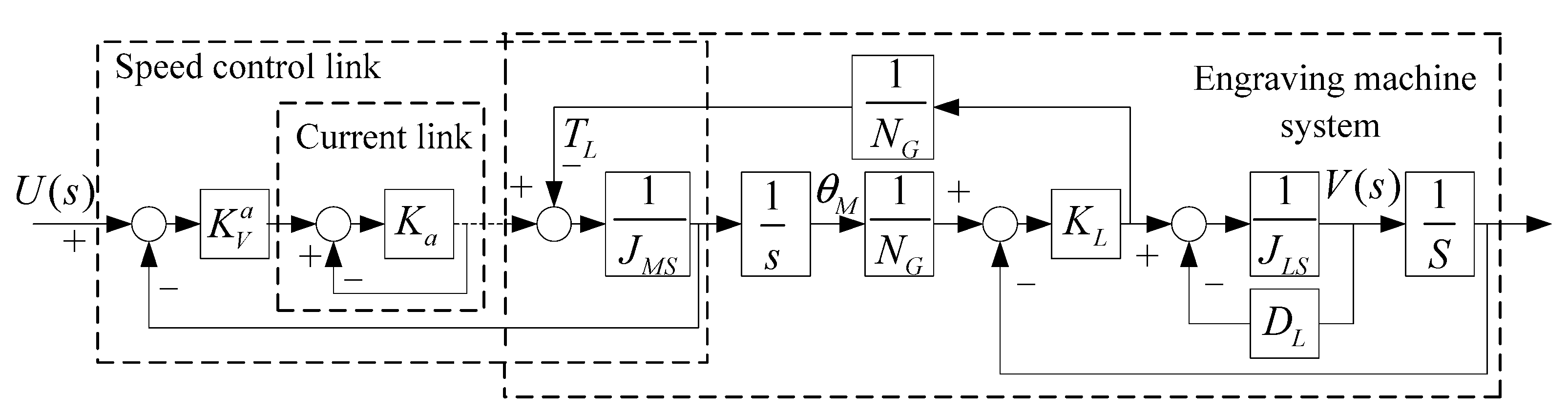
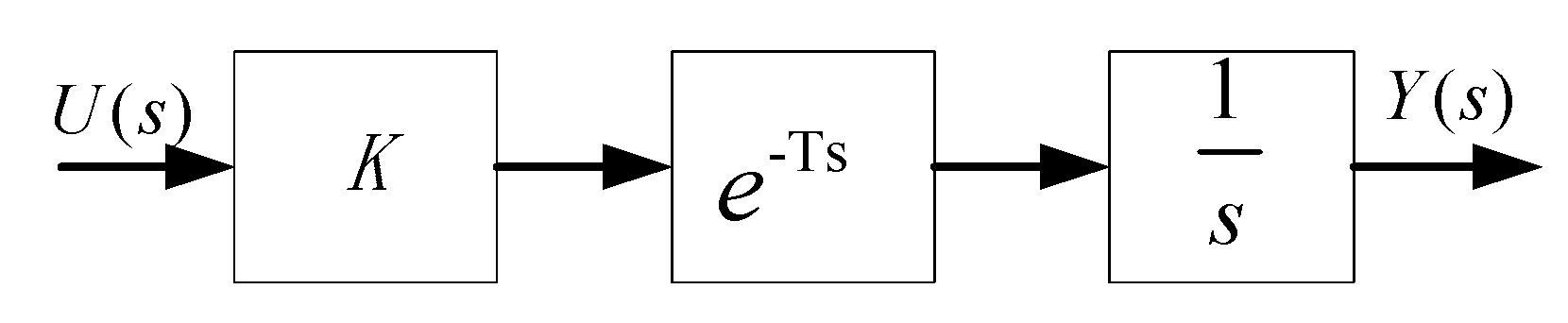
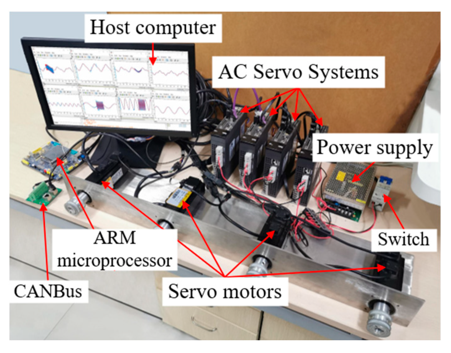
2. Engraving Machine System

The engraving machine system works in a three-dimensional environment, which can move freely forward and back, left and right and up and down. Considering that the mechanism relationship of the three dimensions is almost identical, the operating state of a single axis is considered in this paper. When the servo driver works in the speed mode, the overall structure block diagram of the physical link of the single-axis servo system with the speed as the output is shown in Figure 1.

The transfer function of the system from output $V(s)$ to input $U(s)$ can be obtained using Mason’s equation

$$\begin{array}{l}{G}_{sys}(s)=\frac{U(s)}{V(s)}\\ =K_V^a{K}_a{K}_L/[s^3(1+K_a)J_{\mathrm{M}}{J}_L{N}_G^2+s^2{N}_G^2(J_L{K}_V^a{K}_a+J_{\mathrm{M}}{D}_L+J_{\mathrm{M}}{K}_a{D}_L)+\\ s(J_L{K}_L+N_G^2{K}_V^a{K}_a{D}_L+K_a{K}_L{J}_L+K_a{K}_L{D}_L)+K_a{K}_L{D}_L]\end{array}$$

(1)

where $K_V^a$ is the speed amplification gain; $K_a$ is the current loop gain; $K_L$ is the elastic coefficient; $N_G$ is the ball screw transmission ratio; $J_M$ is the moment of inertia of synchronous servo motor; $J_L$ is the moment of inertia of load and $D_L$ is the coefficient of viscous friction.

The mechanism model shown in Equation (1) can represent the servo system speed model. However, there are many unknown parameters which are difficult to determine precisely. Under the condition of 1/20 rated speed to 1/3 rated speed, the overall structure of the single-axis servo system with angular speed as the input signal and position as the output signal can be effectively simplified, as shown in Figure 2. The simplified model structure can be used to fit and describe the dynamic response of the complex engraving machine system. In general, the system with integral factors can be described using a transfer function, and this function model is not only simple in structure but also conducive to modeling using identification technology.

The transfer function relationship of the simplified model can be expressed as

$$G_{sys}(s)=\frac{Y(s)}{U(s)}=\frac{K{e}^{-Ts}}{s}$$

(2)

where $K$ is the gain and $T$ is the time constant.

When the time constant $T$ is small, Equation (2) can be approximated as

$$G_{sys}(s)=\frac{Y(s)}{U(s)}=\frac{K}{s(Ts+1)}$$

(3)

In the discrete domain, Equation (3) can be estimated using an output error model with an integrating factor

$$y(k)=G_{sys}(z^{-1})=\frac{B(z^{-1})}{(1-z^{-1})A(z^{-1})}u(k)$$

(4)

where $A(z^{-1})=1+a_1{z}^{-1}+\cdots +a_{n_a}{z}^{-n_a}$ and $B(z^{-1})=b_1{z}^{-1}+\cdots +b_{n_b}{z}^{-n_b}$.

During the actual process, the system may also be affected by random measurement noise; Equation (4) is written as

$$\left\{\begin{array}{l}x(k)=\frac{B(z^{-1})}{(1-z^{-1})A(z^{-1})}u(k)\\ y(k)=x(k)+v(k)\end{array}\right.$$

(5)

where $x(k)$ is the noiseless output response and $v(k)$ is the random measurement noise, which is generally defined as Gaussian white noise whose mean is 0 and variance is ${\sigma }^2$.

3. Design of 2-DOF PID Control

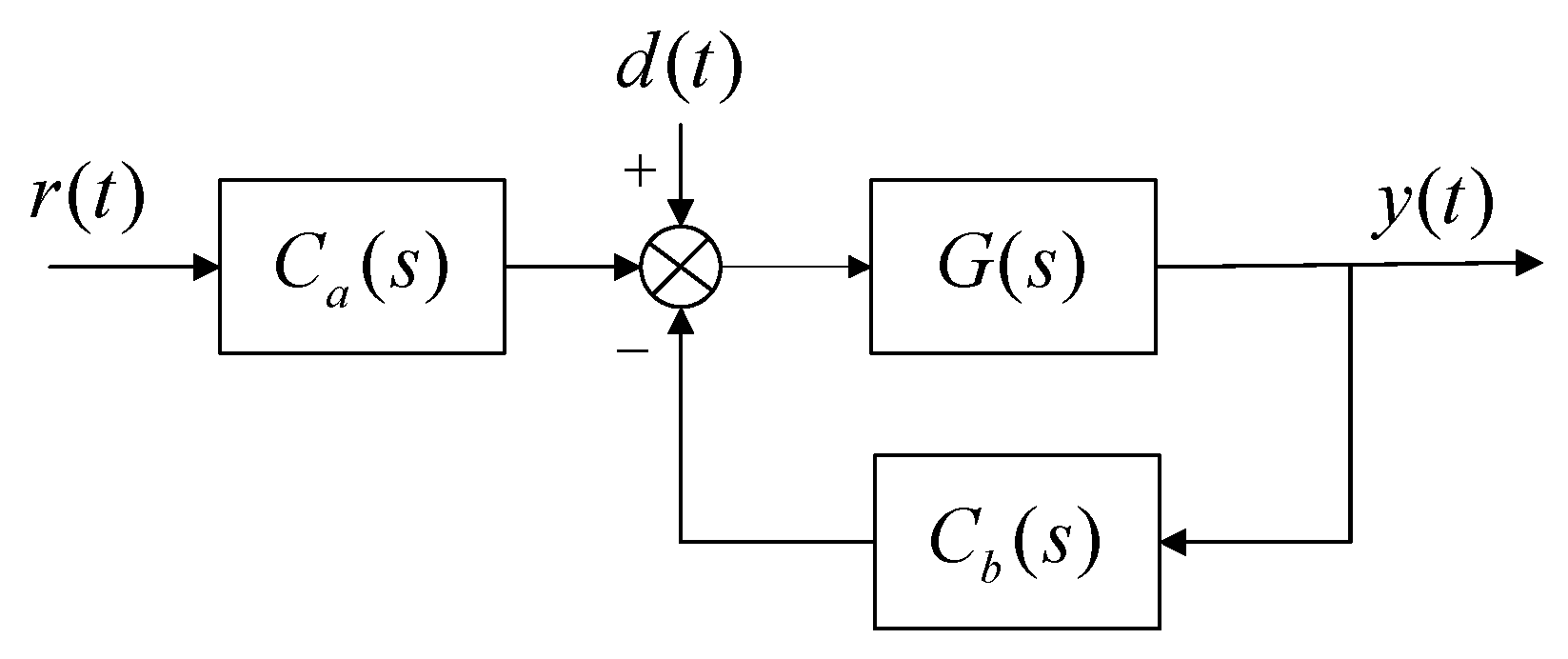
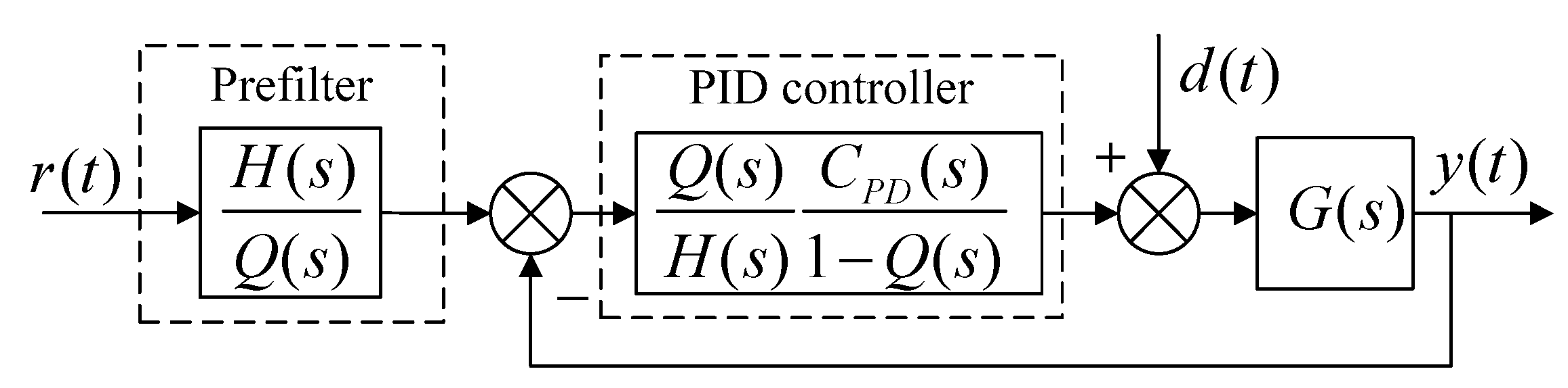
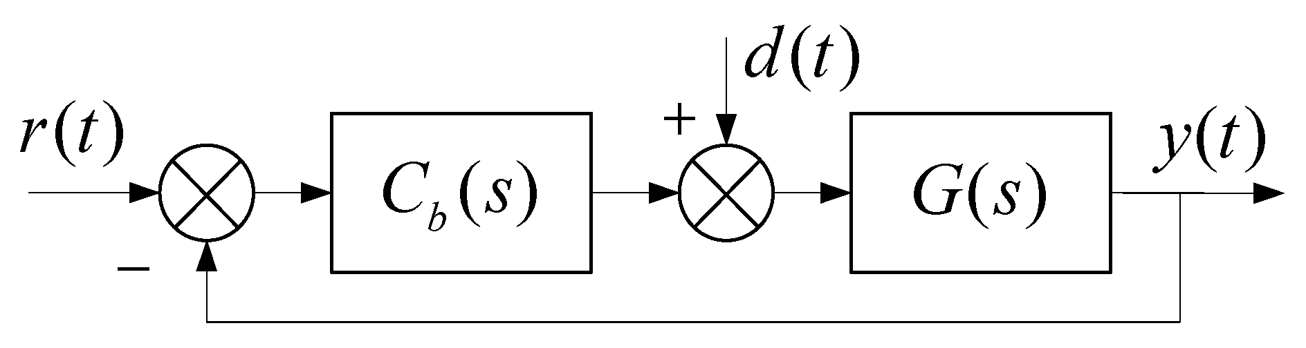
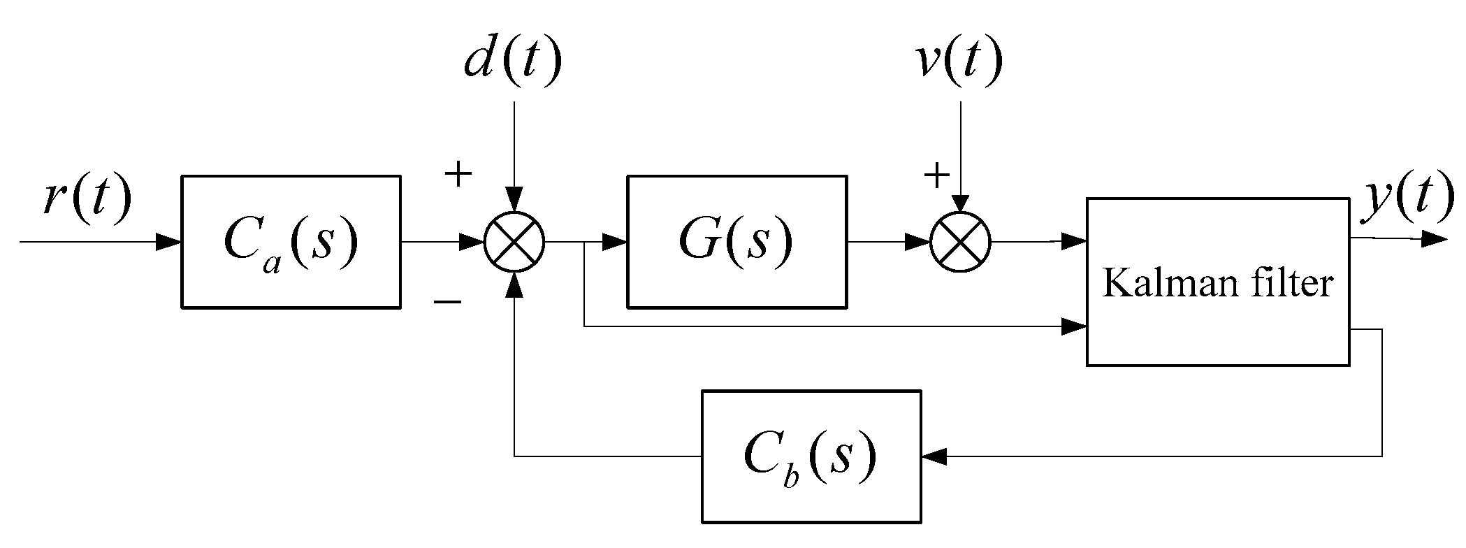
3.1. 2-DOF PID Control Structure

The basic structure of the 2-DOF PID control system adopted in this paper is shown in Figure 3, where $d(t)$ and $v(t)$ are, respectively, input disturbance and output measurement noise. $G(s)$ is the system transfer function; $C_a(s)$ is the set point tracking controller and is also named as the outer loop controller or prefilter, which is used to ensure the set point tracking performance and $C_b(s)$ is the disturbance rejection controller and is also named as the inner loop controller, which is used to reject the influence of input disturbance $d(t)$ on the system.

3.2. Design of Disturbance Rejection Controller

The disturbance rejection (DR) controller $C_b(s)$ is constructed based on the disturbance observer and the expectation model, as shown in Figure 4, where $G(s)$ is a stable transfer function

$$G(s)=\frac{b_{n-l}{s}^{n-l}+b_{n-l-1}{s}^{n-l-1}+\cdots +b_{1}s+b_0}{a_n{s}^n+a_{n-1}{s}^{n-1}+\cdots a_{1}s+a_0}$$

(6)

where $n$ is the denominator order; $l$ is the difference between the numerator order and the denominator order; $H(s)=\frac{1}{{\tau }_{c}s+1}$ is the expected model and ${\tau }_c$ is the time constant of $H(s)$; $Q(s)=\frac{1}{{\tau }_q+1}$ is the low-pass filter and ${\tau }_q$ is the bandwidth of the filter $Q(s)$. $C_{PD}(s)=k_{pd}(1+k_{d}s)$ is the compensator, and its role is to pre-compensate the control input, which helps to enhance the stability of the system. The structure in Figure 4 can also be further represented by the structure in Figure 5, and the converted structure is more convenient for parameter tuning.

For different values of $l$ in the transfer function (6), Figure 5 can be represented in the following PID forms, respectively.

When $l=1$, take $k_{pd}=\frac{a_n}{b_{n-1}{\tau }_c}$, $k_d=0$, then

$$\begin{array}{l}{C}_{PID}(s)=\frac{a_n}{b_{n-1}{\tau }_q}(1+\frac{1}{{\tau }_{c}s})\\ =K(1+\frac{\omega }{s})\end{array}$$

(7)

In this case, the PID parameter can been expressed as

$$\left\{\begin{array}{l}{K}_P^b=K\\ K_I^b=K\omega \\ K_D^b=0\end{array}\right.$$

(8)

where $K=\frac{a_n}{b_{n-1}{\tau }_q}$ determines the disturbance rejection performance of the PID and $\omega =\frac{1}{{\tau }_c}$ determines the closed-loop response speed of the system.

When $l=2$, take $k_{pd}=\frac{a_n}{b_{n-l}{\tau }_c\lambda }$, $k_d=\lambda$, then

$$C_{PID}(s)=\frac{a_n}{b_{n-l}{\tau }_q}(\frac{1}{\lambda }+\frac{1}{{\tau }_c}+\frac{1}{{\tau }_c\lambda s}+s)$$

(9)

and $\frac{H(s)}{Q(s)}$ is a prefilter and used to suppress the system overshoot.

For Equation (9), generally, by taking ${\tau }_c=\lambda$, it can be obtained as follows

$$\begin{array}{l}{C}_{PID}(s)=\frac{a_n}{b_{n-l}{\tau }_q}(\frac{2}{{\tau }_c}+\frac{1}{{\tau }_c{}^{2}s}+s)\\ =K(2\omega +\frac{{\omega }^2}{s}+s)\end{array}$$

(10)

In this case, the PID parameter can be expressed as

$$\left\{\begin{array}{l}{K}_P^b=2K\omega \\ K_I^b=K{\omega }^2\\ K_D^b=K\end{array}\right.$$

(11)

The undetermined parameters $K$ and $\omega$ can be taken in the following way:

(a)

Determine $\omega$ according to the expected closed-loop speed.

(b)

Gradually increase $K$, and gradually improve the control performance until the speed and disturbance rejection performance satisfy the requirements.

(c)

If the system is overshot, the filter $\frac{H(s)}{Q(s)}$ is added to the reference input to suppress the system overshoot.

According to the basic PID structure of two degrees of freedom as shown in Figure 3, the transfer function between the system output $y(t)$ and the input disturbance $d(t)$ is

$$\frac{Y(s)}{D(s)}=\frac{G(s)}{1+G(s)C_b(s)}$$

(12)

This shows that the influence of input disturbance on system output is independent of the set point tracker $C_a(s)$. In order to facilitate designing the disturbance rejection controller $C_b(s)$, the structure in Figure 3 can be equivalent to Figure 6. The controller $C_b(s)$ with disturbance rejection function can be obtained using the design method of the DR-PID mentioned above. When there is overshoot in the system, the pre-controller $C_a(s)$ should be designed.

3.3. Design of the Set Point Tracking Controller

The controller $C_a(s)$ adopts the following PID form

$$C_a(s)=K_P^a+K_I^a/s+K_D^{a}s$$

(13)

The 2-DOF PID methods contains fives parameters to be adjusted, which are difficult to adjust manually. For the three parameters of the set point tracking controller, the DE algorithm with random heuristic characteristics is used to optimize these parameters intelligently. The intelligent algorithm optimization steps are summarized as follows:

(a)

Initialize population parameters:

(1)

Population size $M$: Take the number of individuals $M$ in the population according to demand. In general, the larger the population, the more individuals, the better the search ability. However, it may significantly increase the computation burden, and it is generally selected to be 20 to 50.

(2)

Individual dimension $n$: Take the individual dimension of the population according to the number of optimized parameters. Since the three parameters $K_P^a$, $K_I^a$ and $K_D^a$ need to be adjusted, the $n$ is taken as $n=3$.

(3)

Variation factor $F$: The $F$ determines the population individual differential growth and is used to control population diversity and convergence. The value ranges between 0 and 1. Increasing $F$ can increase the diversity of the population, but it may reduce the convergence speed, and it is easy to jump out of the local extreme value. Reducing $F$ may reduce the difference step size, and it can accelerate the convergence rate such that it will be easier to fall into local optimal values.

(4)

Cross factor $CR$: The $CR$ plays a role in balancing global and local search capabilities, and the value is generally between 0 and 1. Increasing $CR$ can improve the diversity of the population and speed up the convergence rate to a certain extent, but too much crossover operation may have too much impact on the population and reduce the convergence rate. However, reducing $CR$ may reduce the diversity of the population, which not only reduces the convergence speed but also may fall into local optimal values. So, in this paper, the $CR$ is taken between 0.3 and 0.6.

(b)

Generate the initial population: Randomly generate $M$ individuals satisfying the constraint conditions in a space with dimension $n$. The individual generation mode is

$$x_i(j)=x_{\min }(j)+(x_{\max }(j)-x_{\min }(j))ran{d}_{ij}(0,1)$$

(14)

where $x_i(j)$ is the $j\mathrm{th}$ chromosome; $x_{\min }(j)$ and $x_{\max }(j)$ of the $i\mathrm{th}$ individual are the upper and lower bounds of the $j$ chromosome, respectively and $ran{d}_{ij}(0,1)$ is the random number between [0,1].

(c)

Population variation: Three individuals $x_{m1}$, $x_{m2}$ and $x_{m3}$ are randomly selected from the population, and $i\ne m1\ne m2\ne m3$. The basic variation operation is

$$h_i(j)=x_{m1}(j)+F(x_{m2}(j)-x_{m3}(j))$$

(15)

If there is no local optimization problem, two individuals $x_{m2}$ and $x_{m3}$ can be randomly selected from the population, and the mutation operation can be written as

$$h_i(j)=x_b(j)+F(x_{m2}(j)-x_{m3}(j))$$

(16)

where $x_{m2}(j)-x_{m3}(j)$ is the differentiation vector, and this difference operation is the key to the differential evolution algorithm; $F$ is the variation factor, indicating the degree of scaling; and $x_b(j)$ is the $j$ chromosome information of the best individual in the population in the current generation. Since Equation (16) draws on the best individual chromosome information in the current population, the convergence rate can be accelerated.

(d)

Population crossover: The operation of crossover increases the diversity and randomness of the population. The specific operations are

$$v_i(j)=\left\{\begin{array}{l}{h}_i(j),rand l_{ij}\le CR\\ x_i(j),rand l_{ij}>CR\end{array}\right.$$

(17)

where $rand l_{ij}$ is the random number between [0,1]; $CR$ is the crossover probability and $CR\in [0,1]$.

(e)

Selection operation: To determine whether $x_i(j)$ becomes a member of the next generation, compare the fitness function of the crossed vector $v_i(j)$ and the target vector $x_i(j)$.

$$x_i(j)=\left\{\begin{array}{l}{v}_i(j), f(v_i(1),\cdots ,v_i(n))<f(x_i(1),\cdots ,x_i(n))\\ x_i(j), f(v_i(1),\cdots ,v_i(n))\ge f(x_i(1),\cdots ,x_i(n))\end{array}\right.$$

(18)

Repeat steps 2–5 until the maximum evolutionary algebra $G$ is reached.

Since the controller $C_a(s)$ is mainly used to improve the set point tracking performance of the system, the following fitness function equation is used to evaluate the performance of the individuals in the population

$$f={\displaystyle \sum _{k=1}^N|e(k)|}$$

(19)

where $e(k)=r(k)-y(k)$; $r(k)$ is the expected tracking value and $y(k)$ indicates the system output value. Considering that the prefilter is not set when the disturbance rejection controller is designed to suppress the appearance of system overshoot, the fitness Function (19) is modified as

$$f(k)=\left\{\begin{array}{l}f(k-1)+|e(k)|, e(k)\ge 0\\ f(k-1)+\eta |e(k)|, e(k)<0\end{array}\right.$$

(20)

When the system produces overshoot, which means $e(k)<0$, $\eta |e(k)|(\eta >1)$ is used to produce a larger fitness function value to punish the population individuals at this time, thus inhibiting the overshoot.

During the actual production process, the system will not only be affected by the input disturbance $d(t)$, but also the output measurement data may contain random measurement noise $v(t)$, which will be suppressed by the Kalman filter algorithm in this paper. It should be noted that the proposed control algorithm involves many undetermined parameters. It is necessary to test the step signal or pulse signal of the system to obtain the dynamic characteristics and types of the system. The tuning of PID parameters needs to consider the rapidity, stability and accuracy of the system response. Then the intelligent differential evolution algorithm is used for parameter optimization and tuning. Moreover, the parameters of the intelligent optimization algorithm should not only satisfy the optimization requirements but also not have too long of a calculation time.

4. Kalman Filtering Algorithm

Consider the following general state space model

$$\left\{\begin{array}{l}x(k)=Ax(k-1)+B(u(k)+w(k))\\ z(k)=Hx(k)+v(k)\end{array}\right.$$

(21)

where $x(k)$ and $x(k-1)$ are the system state at time $k$ and time $k-1$, respectively; $u(k)$ is the system input; $z(k)$ is the observed quantity of the system; $A$ is the state transition matrix; $B$ is the control input matrix; $H$ is the state observation matrix; $w(k)$ is the process noise, which is used to compensate for the error between the estimated state and the real state; and $v(k)$ is the measurement noise.

Because precise information about the process noise and measurement noise is often unknown, at $k-1$ time, only one step recursion can be performed to obtain a prior estimate of the state of $k$ moment. Given

$${\tilde{x}}^{-}(k)=A\tilde{x}(k-1)+Bu(k)$$

(22)

Define the best estimate as

$$\tilde{x}(k)={\tilde{x}}^{-}(k)+K(z(k)-H{\tilde{x}}^{-}(k))$$

(23)

where $K$ is the Kalman coefficient, representing the weight of the prior estimate ${\tilde{x}}^{-}(k)$ and the posterior observation $z(k)$ in the final optimal estimate. Define the prior error as

$$e_f^{-}(k)=x(k)-{\tilde{x}}^{-}(k)$$

(24)

Define its covariance matrix as

$$P^{-}(k)=E(e_f^{-}(k)e_f^{-}{(k)}^T)$$

(25)

Define a posterior error

$$e_f(k)=x(k)-\tilde{x}(k)$$

(26)

Define its covariance matrix as

$$P(k)=E(e_f(k)e_f{(k)}^T)$$

(27)

The $P^{-}(k)$ and $P(k)$ are symmetric matrices. When the posterior error $e_f(k)$ reaches the minimum and the best estimate $\tilde{x}(k)$ is closest to the true value $x(k)$, rewrite Equation (26) as

$$\begin{array}{l}{e}_f(k)=x(k)-\tilde{x}(k)\\ =x(k)-({\tilde{x}}^{-}(k)+K(z(k)-H{\tilde{x}}^{-}(k)))\\ =(I-KH)e_f^{-}(k)-Kv(k)\end{array}$$

(28)

Then

$$\begin{array}{l}P(k)=E(e_f(k)e_f{(k)}^T)\\ =E(((I-KH)e_f^{-}(k)-Kv(k))\ast \\ {((I-KH)e_f^{-}(k)-Kv(k))}^T)\end{array}$$

(29)

Assume $v(k)$ is Gaussian white noise with expectation 0 and variance $R$, then

$$\begin{array}{l}P(k)=E(((I-KH)e_f^{-}(k)+Kv(k))\ast \\ {((I-KH)e_f^{-}(k)+Kv(k))}^T)\\ =P^{-}(k)-P^{-}(k)H^T{K}^T-KH{P}^{-}(k)+\\ K(H{P}^{-}(k)H^T+R)K^T\end{array}$$

(30)

In order to minimize the error between the best estimate and the true value, the objective function is taken as

$$J=\min tr(P(k))$$

(31)

The partial derivative of Equation (31) with respect to the Kalman coefficient $K$ can be expressed as

$$\frac{\partial tr(P(k))}{\partial K}=-2P^{-}(k)H^T+2K(H{P}^{-}(k)H^T+R)$$

(32)

Set Equation (32) to zero and we have

$$K=P^{-}(k)H^T{(H{P}^{-}(k)H^T+R)}^{-1}$$

(33)

Substitute Equation (33) into Equation (30) and $P(k)$ can be updated as follows

$$P(k)=(I-KH)P^{-}(k)$$

(34)

For $P^{-}(k)$, we have

$$\begin{array}{l}{P}^{-}(k)=E(e_f^{-}(k)e_f^{-}{(k)}^T)\\ =E((A{e}_f(k-1)+Bw(k)){(A{e}_f(k-1)+Bw(k))}^T)\end{array}$$

(35)

Assume that $w(k)$ is Gaussian white noise with an expectation of 0 and a variance of $Q$, then

$$\begin{array}{l}{P}^{-}(k)=E((A{e}_f(k-1)+Bw(k)){(A{e}_f(k-1)+Bw(k))}^T)\\ =AP(k-1)A^T+BQ{B}^T\end{array}$$

(36)

The Kalman filtering algorithm steps are summarized as follows:

• According to the discrete state space model of the system, the matrix $A$, $B$, $H$ is obtained, and $P(0)$ and $\tilde{x}(0)$ are initialized.
• The covariance matrices $Q$ and $R$ of $w(k)$ and $v(k)$ are set reasonably according to the system characteristics and actual environment.
• Obtain a prior estimate

$${\tilde{x}}^{-}(k)=A\tilde{x}(k-1)+Bu(k)$$

(37)

4.

Update the prior covariance $P^{-}(k)$

$$P^{-}(k)=AP(k-1)A^T+BQ{B}^T$$

(38)

5.

Calculate the Kalman gain $K$

$$K=P^{-}(k)H^T{(H{P}^{-}(k)H^T+R)}^{-1}$$

(39)

6.

Compute the best estimate (posterior estimate) $\tilde{x}(k)$

$$\tilde{x}(k)={\tilde{x}}^{-}(k)+K(z(k)-H{\tilde{x}}^{-}(k))$$

(40)

7.

Update the posterior covariance matrix $P(k)$

$$P(k)=(I-KH)P^{-}(k)$$

(41)

8.

Repeat steps 3–7 to achieve the desired target.

The block diagram of the proposed control algorithm can be summarized as shown in Figure 7. Note that when designing the disturbance rejection controller $C_b(s)$, the controlled plant should be a linear system. Moreover, ref. [29] shows that that the nonlinear system can be processed using linear approximation technology to satisfy the design requirements of the disturbance rejection controller. In addition, the extended Kalman filter or untraced Kalman filter can be used to filter the nonlinear system. Furthermore, the parameter tuning is solved using intelligent optimization technology, which can avoid the instability problem of a manual parameter setting. Therefore, the control algorithm proposed in this paper can ensure that the system is stable.

5. Simulation and Experimental Verification

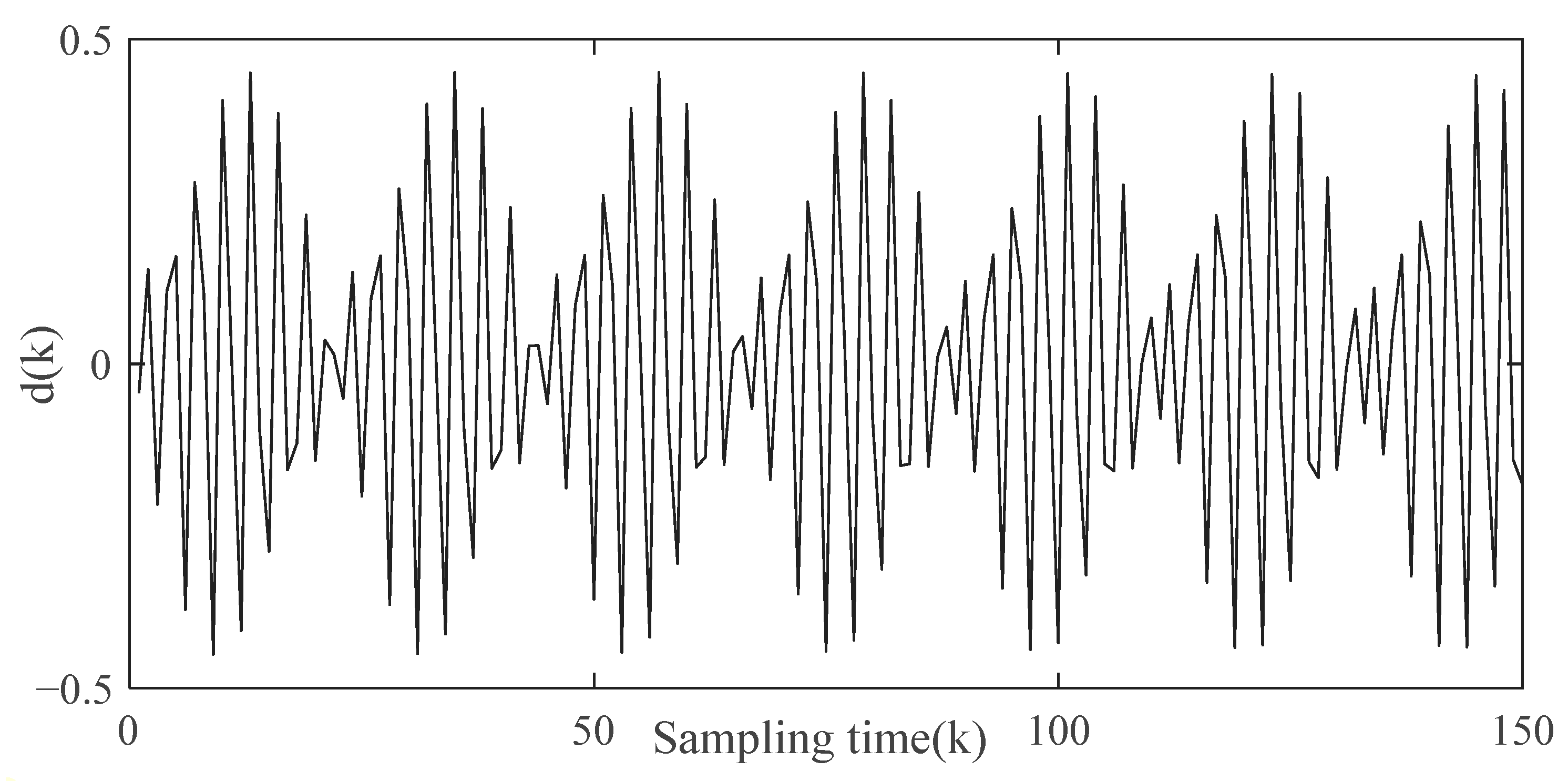
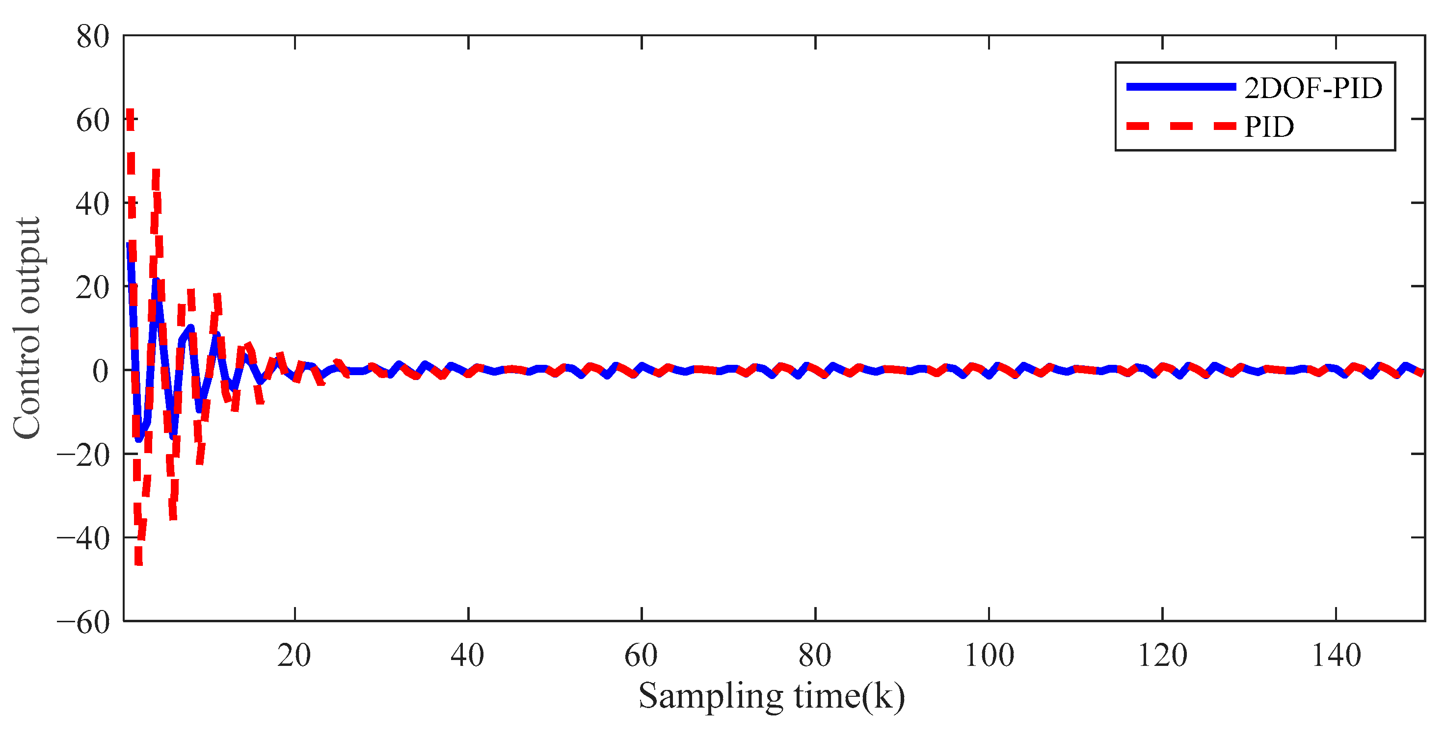
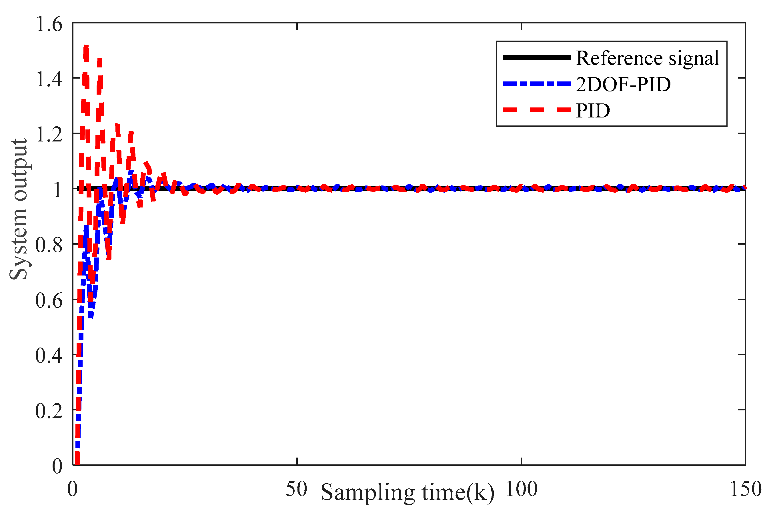
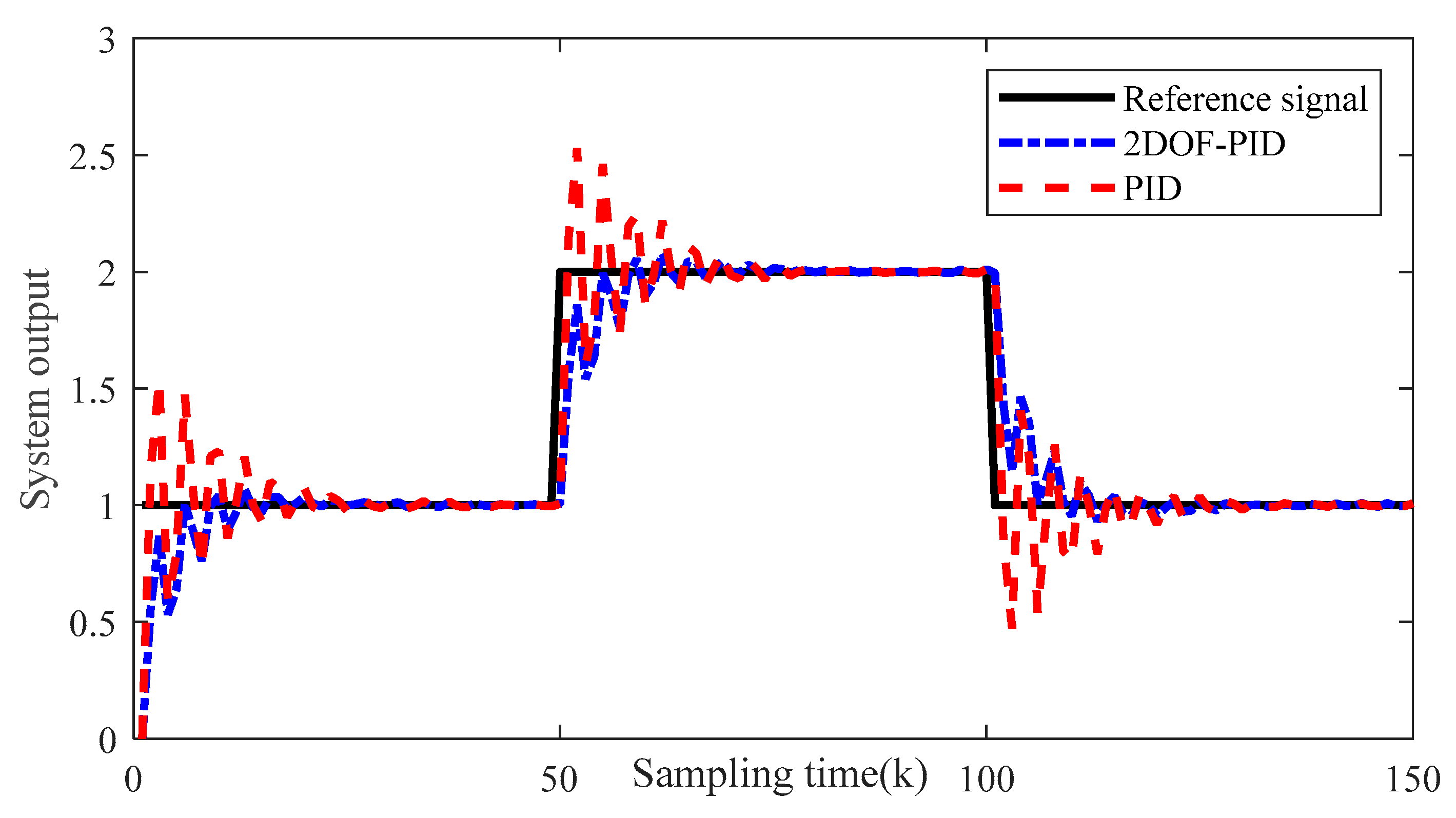
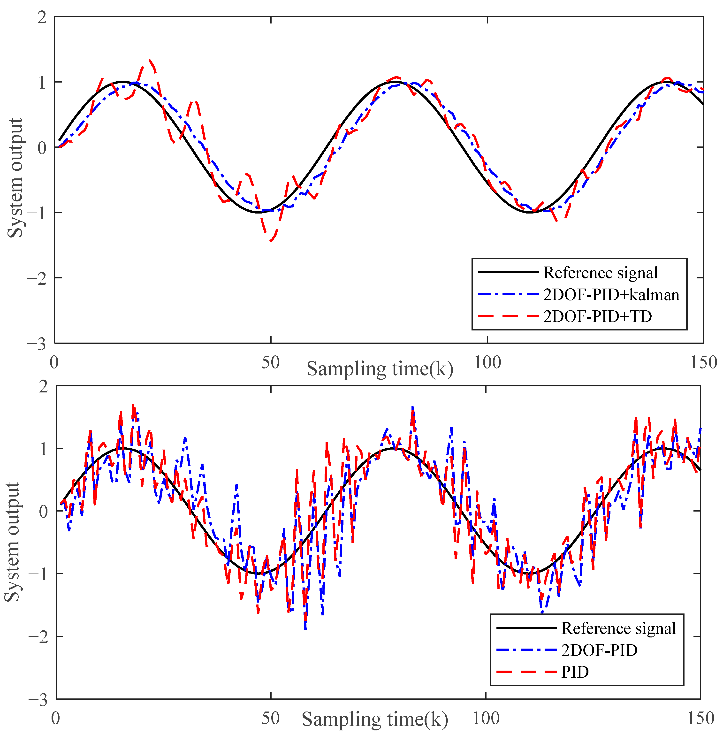
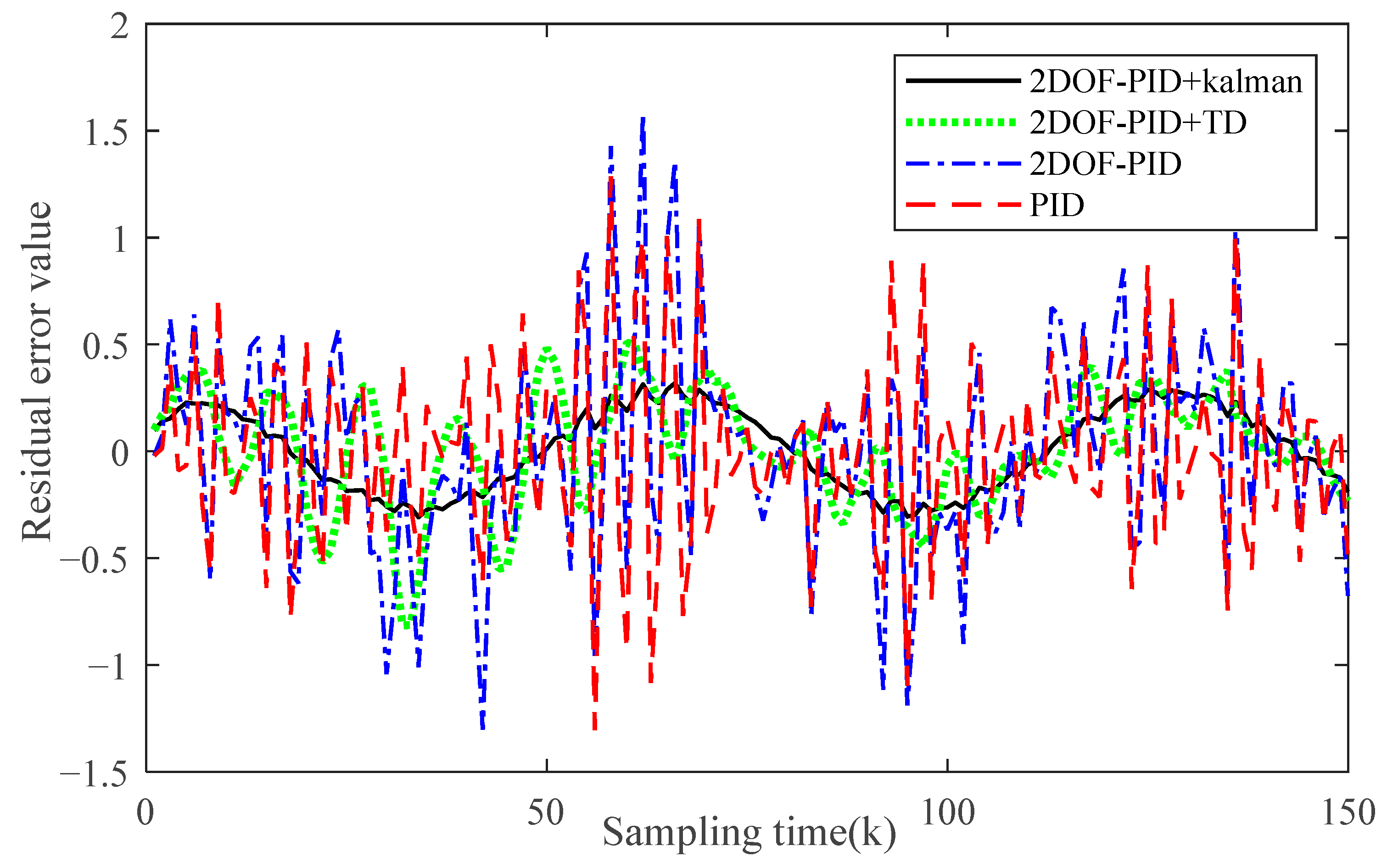
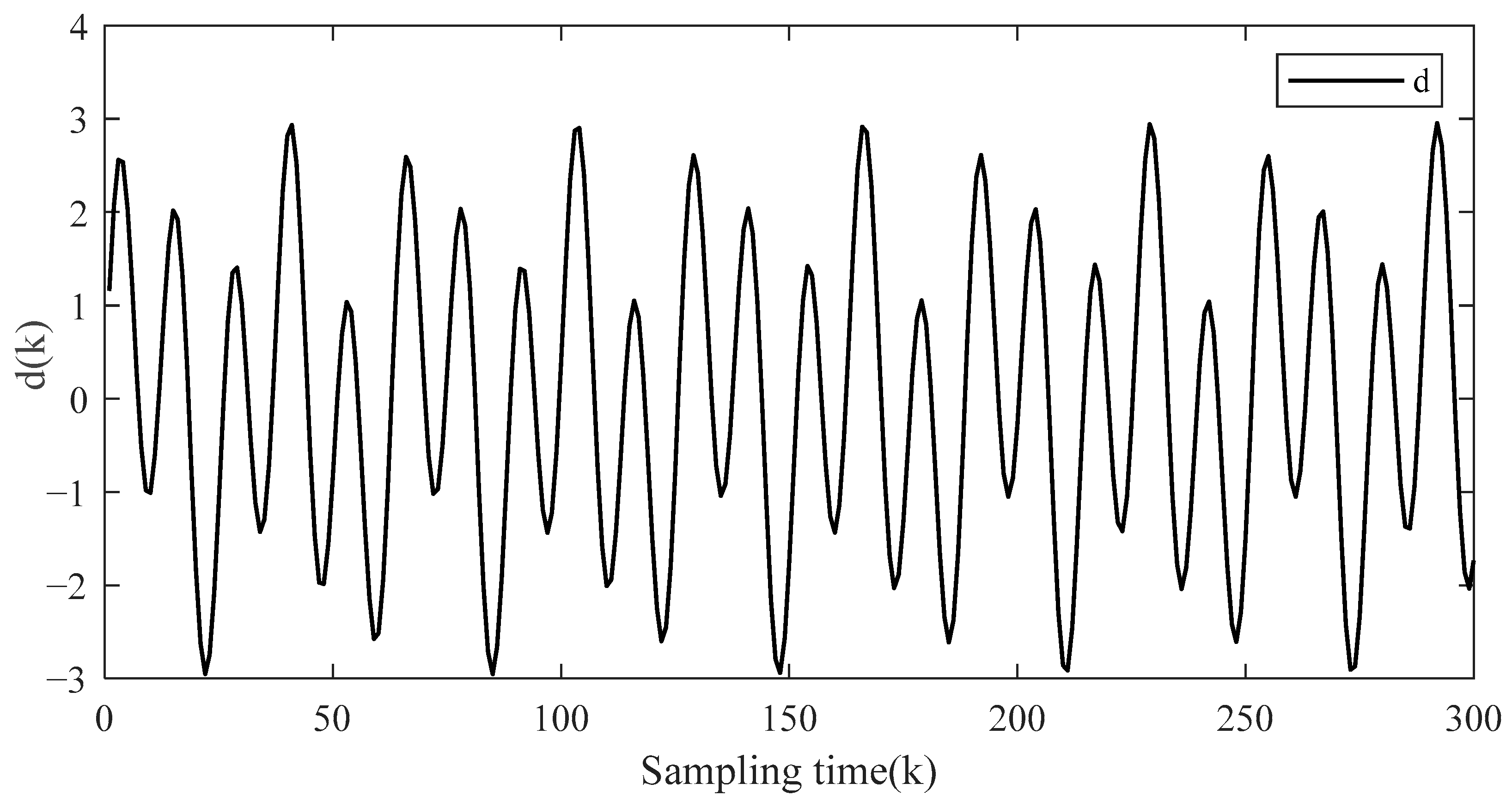
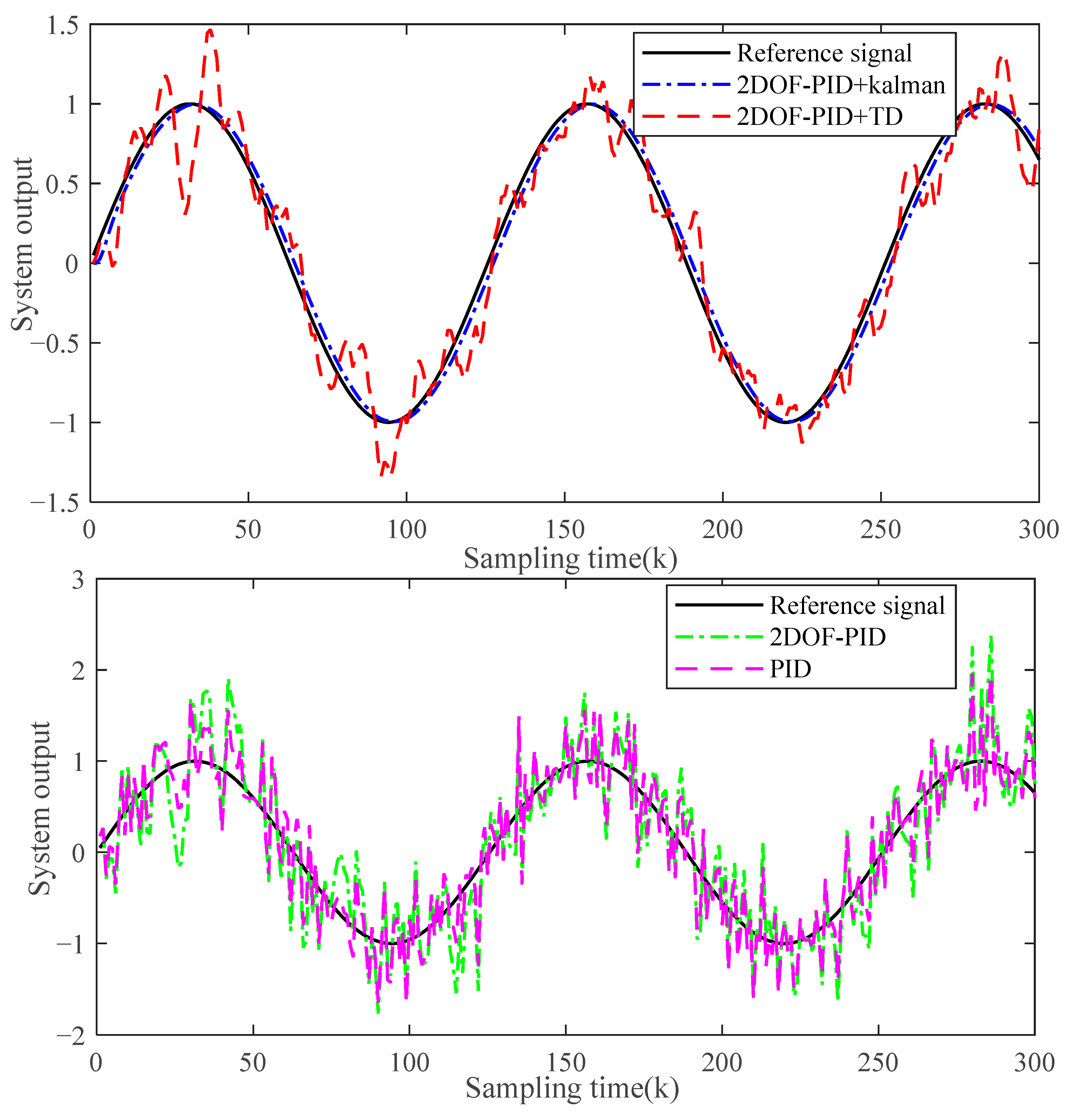
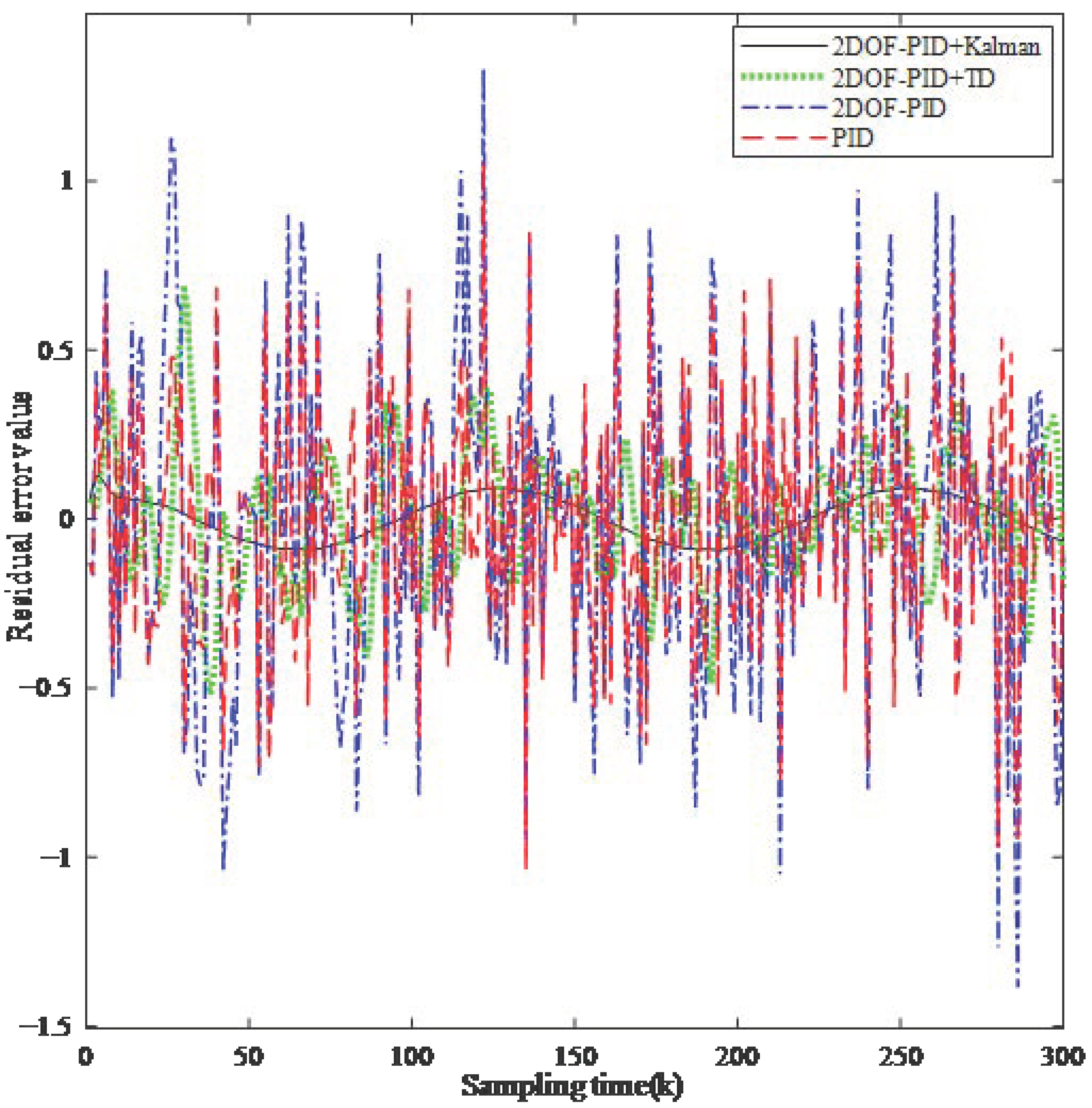
5.1. Numerical Simulation

Consider the following systems

$$\frac{y(z)}{u(z)}=\frac{0.01839z+0.01321}{(z-1)(z-0.3689)}$$

(42)

They can be converted into the following discrete state space model

$$\left\{\begin{array}{l}\left[\begin{array}{l}x(k-1)\\ x(k)\end{array}\right]=\left[\begin{array}{cc}0& 1\\ 1.3679& 0.3679\end{array}\right]\left[\begin{array}{c}x(k-2)\\ x(k-1)\end{array}\right]\\ +\left[\begin{array}{cc}0& 0\\ 0.01321& 0.01839\end{array}\right]\left[\begin{array}{l}u(k-2)\\ u(k-1)+w(k)\end{array}\right]\\ y(k)=[\begin{array}{cc}0& 1\end{array}]\left[\begin{array}{l}x(k-1)\\ x(k)\end{array}\right]+v(k)\end{array}\right.$$

(43)

where $x(k)$ and $x(k-1)$ are the system state at time $k$ and time $k-1$, respectively; $y(k)$ is the output measurement value; and $u(k-1)$ and $u(k-2)$ are the system control inputs at $k-1$ time and $k-2$ time, respectively. $w(k)$ is Gaussian white noise with mean 0 and variance 0.25. The sampling point is $N=150$. The step is taken as $t_s=0.05$. The total simulation time is taken as 7.5 s. $d(k)$ is taken as

$$d(k)=0.2\sin (2k)+0.3\sin (4k)$$

(44)

The dynamic input disturbance $d(k)$ is shown in Figure 8.

The proposed 2-DOF PID control method based on the Kalman filter is used to control the above system. Since the order difference between the numerator and denominator is $l=2$, Equation (10) is used to design the disturbance rejection controller $C_b(s)$. By setting $K=2$ and $\omega =5$, $K_P^b$, $K_I^b$ and $K_D^b$ can be calculated as $K_P^b=20$, $K_I^b=50$ and $K_D^b=2$ using Equation (11). For the set point tracking controller $C_a(s)$, the parameters of the differential evolution algorithm are taken as variation factor $F=1.0$, crossover factor $cr=0.8$, number of population individuals $M=30$, number of iterations $G=50$, fitness function is set to the form shown in Equation (20) and $\eta =3$. The parameters of the set point tracking controller are calculated to be $K_P^a=13.3955$, $K_I^a=49.9995$ and $K_D^a=0.7328$. The reference signal $r(k)$ is taken as

$$r(k)=1$$

(45)

The disturbance rejection performances of single-degree-of-freedom PID control and 2-DOF PID control are compared in Figure 9 and Figure 10. When a disturbance $d(k)$ is added to the system, the control input signals of the two control algorithms are shown in Figure 8. The control output response signals of the two control algorithms are shown in Figure 9. It can be seen that the single-degree-of-freedom PID has the same input disturbance rejection performance as the 2-DOF PID.

In order to compare the tracking performance of different algorithms for time-varying signals, the reference control signal $r(k)$ is taken as

$$r(k)=\left\{\begin{array}{l}1 , 0\le k\le 50 , 100\le \mathrm{k}\le 150\\ 2 , 50\le k\le 100\end{array}\right.$$

(46)

The set point tracking capabilities of the two control methods are shown in Figure 11. Figure 11 shows that the 2-DOF PID has better set point tracking performance.

In order to compare and highlight the output noise suppression performance of the proposed control algorithm, it is assumed that the system is subjected to Gaussian white noise $v(k)$ with an expectation of 0 and a variance of 0.04. The tracking results of different control algorithms for the system output with measurement noise are shown in Figure 12, where the tracking differentiator speed factor is taken as $\delta =100$ and the filter factor is taken as $h_0=0.12$. The reference signal $r(k)$ is taken as

$$r(k)=\sin (0.1k)$$

(47)

In order to quantitatively evaluate the control effect of different control algorithms, the integral absolute error (IAE) of tracking error is defined as

$$G_{IAE}(k)={\displaystyle \sum _{k=1}^n|r(k)-y(k)|}$$

(48)

where $r(k)$ is the reference signal and $y(k)$ is the actual output signal.

The residual error values of different control algorithms are shown in Figure 13. The cumulative control error results of different control algorithms are shown in Figure 14. We can see that the single-degree-of-freedom PID control algorithm struggles to suppress the influence of output measurement noise. Although the basic 2-DOF PID control algorithm can take into account the performance of input disturbance rejection and set point tracking, it makes up for the defect of the single-degree-of-freedom PID algorithm which can only guarantee one performance. However, when the system output is subject to random noise, the 2-DOF PID control algorithm cannot effectively suppress the uncertainty caused by the output noise. When the output $y(k)$ of the system is subjected to measurement noise, for the 2-DOF PID control algorithm without the filter, the differential processing of $y(k)$ by the controller $C_b$ may amplify the noise variance. The output $y(k)$ with noise is processed directly by the 2-DOF PID controller. Single-degree-of-freedom PID processes the difference between the output $y(k)$ containing noise and the reference signal $r(k)$, which results in less noise influence on the control result. The tracking differentiator is used to process the system output; it can be seen from Figure 11 and Figure 12 that there is still a large tracking error. The proposed 2-DOF PID control algorithm based on the Kalman filter can not only retain the input disturbance rejection performance and set point tracking performance of 2-DOF PID but also effectively suppress the uncertainty influence caused by output noise.

5.2. Experimental Example

The engraving machine system used for testing is shown in Figure 15. The detailed parameter configuration of the experimental platform is shown in

Table 1. Parameter configuration of platform.

Parameter Name	Configuration
CPU	Core i5-4210M 2.6 GHz
RAM	8 GM
Operating system	Windows10 64 bit
Embedded interface board chip	STM32F407ZGT6 168M Hz
Ethernet communication rate	100 Mb/s
CAN communication rate	1 Mb/s
Sampling period	1 ms–5 ms
AC server	DeltaASDA-A2
Permanent magnet synchronous motor	DeltaECMA-C10604RS
Electronic gear ratio	1/128 (10,000 pulses/cycles)
Sensor position accuracy	5 × 10−4 mm
Range of liabilities for hysteresis	−10 N–10 N

. When the driver works in speed mode, the system can be regarded as a three-axis servo system with angular speed as the input and position as the output. For the same actuator, the mechanism relationship of the three axes is the same, and the X-axis will be controlled in this paper. The engraving machine system can be modeled by the discrete state space model

$$\left\{\begin{array}{l}\left[\begin{array}{l}x(k-1)\\ x(k)\end{array}\right]=\left[\begin{array}{cc}0& 1\\ 0.6907& 1.6907\end{array}\right]\left[\begin{array}{l}x(k-2)\\ x(k-1)\end{array}\right]\\ +\left[\begin{array}{l}0\\ 1.2868\ast {10}^{-4}\end{array}\right](u(k-1)+w(k))\\ y(k)=\left[\begin{array}{cc}1& 0\end{array}\right]\left[\begin{array}{l}x(k-1)\\ x(k)\end{array}\right]+v(k)\end{array}\right.$$

(49)

where $x(k)$ is the system state. The system input $u(k)$ is the target torque (unit: one rated torque in a thousand) stored in the register. The system output $y(k)$ is the velocity (unit: centimeter, cm). The portion of input and output data are at a sampling frequency of 100 Hz.

Because the difference between the numerator and denominator order of the transfer function of the engraving machine system is $l=2$, Equation (10) is used to design $C_b(s)$. Take $K=100$, $\omega =4.5$. The parameters of controller $C_b(s)$ are taken as $K_P^b=900$, $K_I^b=2025$ and $K_D^b=100$. For the differential evolution algorithm, the parameters are taken as $F=1.0$, $cr=0.8$, $M=30$, $G=50$ and $\eta =2$. The parameters of controller $C_a(s)$ can be obtained as $K_P^a=705.9$, $K_I^a=2025.8$ and $K_D^a=149.6$.

In order to highlight the disturbance rejection performance of different algorithms, the input disturbance signal $d(k)$ is artificially taken as

$$d(k)=2\sin (0.5k)+\sin (0.2k)$$

(50)

The dynamic input disturbance $d(k)$ is shown in Figure 16.

The reference signal $r(k)$ is taken as

$$r(k)=\sin (0.05k)$$

(51)

The parameters of the tracking differentiator are set to speed factor $\delta =80$ and filter factor $h_0=0.1$. The control results of different control algorithms are shown in Figure 17. The residual error values of different control algorithms are shown in Figure 18. The cumulative tracking errors generated by different algorithms are shown in Figure 19. It can be seen that the proposed 2-DOF PID control algorithm can better suppress the input disturbance and the output measurement noise. The experimental system test shows that the proposed control algorithm has good industrial practicability. In contrast, it is difficult for other control algorithms to obtain satisfactory control accuracy and control stability, which seriously affects their practical application.

6. Conclusions

For an engraving machine system with an integrating factor subject to input disturbance and output measurement noise, a disturbance rejection controller based on an observer and expectation model is designed to reject the influence of input disturbance. Based on the structure of the single-degree-of-freedom PID control strategy, a prefilter is added to ensure the set point tracking performance of the system. The IAE is used as the fitness function of the DE algorithm and the prefilter parameters are optimized intelligently. The adaptive control error weight adjustment parameters are taken to suppress the possible overshoot during the control process. The Kalman filter algorithm is used to process the output measurement signal to suppress the adverse effects of the noise contained in the output measurement signals, and the estimated signal of the system output is obtained simultaneously. Finally, the effectiveness of the proposed 2-DOF PID control algorithm has been verified experimentally by comparing it with existing algorithms. The linear approximation technique can be used to simplify the nonlinear system, and the proposed control algorithm can be used to design the controller. And the control effect can be effectively improved by combining the extended Kalman filter or untraced Kalman filter. For multi-input and multi-output systems, the control strategy presented in this paper can also be studied by combining decoupling technology.

References

1. Durna, A.; Fries, J.; Hrabovsky, L.; Sliva, A.; Zarnovsky, J. Research and development of laser engraving and material cutting machine from 3D printer. Manag. Syst. Prod. Eng. 2020, 1, 47–52. [Google Scholar] [CrossRef]
2. Yang, Z.; Cui, W.; Zhang, W.; Wang, Z.; Zhang, B.; Chen, Y.; Hu, N.; Bi, X.; Hu, W. A new performance optimization method for linear motor feeding system. Actuators 2023, 12, 233. [Google Scholar] [CrossRef]
3. Dong, H.; Zhang, Q.; Xiang, W.U.; Yansui, W.U. Contour error control of CNC engraving machine system based on ADRC. J. Syst. Sci. Math. Sci. 2019, 39, 1001. [Google Scholar]
4. Rodriguez, J.; Garcia, C.; Mora, A.; Flores-Bahamonde, F.; Acuna, P.; Novak, M.; Zhang, Y.; Tarisciotti, L.; Davari, S.A.; Zhang, Z.; et al. Latest advances of model predictive control in electrical drives—Part I: Basic concepts and advanced strategies. IEEE Trans. Power Electron. 2021, 37, 3927–3942. [Google Scholar] [CrossRef]
5. Ju, X.; Lu, J.; Rong, B.; Jin, H. Parameter identification of displacement model for giant magnetostrictive actuator using differential evolution algorithm. Actuators 2023, 12, 76. [Google Scholar] [CrossRef]
6. Das, D.; Chakraborty, S.; Naskar, A.K. Controller design on a new 2DOF PID structure for different processes having integrating nature for both the step and ramp type of signals. Int. J. Syst. Sci. 2023, 54, 1423–1450. [Google Scholar] [CrossRef]
7. Sariyildiz, E.; Oboe, R.; Ohnishi, K. Disturbance observer-based robust control and its applications: 35th anniversary overview. IEEE Trans. Ind. Electron. 2019, 67, 2042–2053. [Google Scholar] [CrossRef]
8. Guras, R.; Strambersky, R.; Mahdal, M. The PID and 2DOF control of the integral system-influence of the 2DOF parameters and practical implementation. Meas. Control 2022, 55, 94–101. [Google Scholar] [CrossRef]
9. Lim, S.; Yook, Y.; Heo, J.P.; Im, C.G.; Ryu, K.H.; Sung, S.W. A new PID controller design using differential operator for the integrating process. Comput. Chem. Eng. 2023, 170, 108105. [Google Scholar] [CrossRef]
10. Yu, S.; Hao, G. On a Vision-based manipulator simulator. Actuators 2023, 12, 78. [Google Scholar] [CrossRef]
11. Jin, Q.B.; Liu, Q. Analytical IMC-PID design in terms of performance/robustness tradeoff for integrating processes: From 2-Dof to 1-Dof. J. Process Control. 2014, 24, 22–32. [Google Scholar] [CrossRef]
12. Xia, T.; Zhang, Z.; Hong, Z.; Huang, S. Design of fractional order PID controller based on minimum variance control and application of dynamic data reconciliation for improving control performance. ISA Trans. 2023, 133, 91–101. [Google Scholar] [CrossRef] [PubMed]
13. Chen, L.; Li, Z.; Yang, J.; Song, Y. Lateral stability control of four-wheel-drive electric vehicle based on coordinated control of torque distribution and ESP differential braking. Actuators 2021, 10, 135. [Google Scholar] [CrossRef]
14. Gorez, R. New design relations for 2-DOF PID-like control systems. Automatica 2003, 39, 901–908. [Google Scholar] [CrossRef]
15. Alfaro, V.M.; Vilanova, R.; Arrieta, O. Robust tuning of Two-Degree-of-Freedom (2-DoF) PI/PID based cascade control systems. J. Process Control 2009, 19, 1658–1670. [Google Scholar] [CrossRef]
16. Sahu, R.K.; Panda, S.; Rout, U.K. DE optimized parallel 2-DOF PID controller for load frequency control of power system with governor dead-band nonlinearity. Int. J. Electr. Power Energy Syst. 2013, 49, 19–33. [Google Scholar] [CrossRef]
17. Gün, A. Attitude control of a quadrotor using PID controller based on differential evolution algorithm. Expert Syst. Appl. 2023, 229, 120518. [Google Scholar] [CrossRef]
18. Jiang, R.; Shankaran, R.; Wang, S.; Chao, T. A proportional, integral and derivative differential evolution algorithm for global optimization. Expert Syst. Appl. 2022, 206, 117669. [Google Scholar] [CrossRef]
19. Yunjun, C.; Chao, J.; Jiuzhi, D.; Zhanshan, Z. Output feedback sliding mode control based on adaptive sliding mode disturbance observer. Meas. Control 2022, 55, 646–656. [Google Scholar] [CrossRef]
20. Han, J. From PID to active disturbance rejection control. IEEE Trans. Ind. Electron. 2009, 56, 900–906. [Google Scholar] [CrossRef]
21. Fu, T.; Gao, Y.; Guan, L.; Qin, C. An LADRC controller to improve the robustness of the visual tracking and inertial stabilized system in luminance variation conditions. Actuators 2022, 11, 118. [Google Scholar] [CrossRef]
22. Zhang, H.; Xiao, G.; Yu, X.; Xie, Y. On convergence performance of discrete-time optimal control based tracking differentiator. IEEE Trans. Ind. Electron. 2020, 68, 3359–3369. [Google Scholar] [CrossRef]
23. Wang, C.; Ji, X.; Zhang, Z.; Zhao, B.; Quan, L.; Plummer, A.R. Tracking differentiator based back-stepping control for valve-controlled hydraulic actuator system. ISA Trans. 2022, 119, 208–220. [Google Scholar] [CrossRef] [PubMed]
24. Micić, A.D.; Mataušek, M.R. Optimization of PID controller with higher-order noise filter. J. Process Control 2014, 24, 694–700. [Google Scholar] [CrossRef]
25. Ahn, K.K.; Truong, D.Q. Online tuning fuzzy PID controller using robust extended Kalman filter. J. Process Control 2009, 19, 1011–1023. [Google Scholar] [CrossRef]
26. Truong, D.Q.; Ahn, K.K. Force control for press machines using an online smart tuning fuzzy PID based on a robust extended Kalman filter. Expert Syst. Appl. 2011, 38, 5879–5894. [Google Scholar] [CrossRef]
27. Segovia, V.R.; Hägglund, T.; Åström, K. Measurement noise filtering for PID controllers. J. Process Control 2014, 24, 299–313. [Google Scholar] [CrossRef]
28. Chen, Y.W.; Tu, K.M. Robust self-adaptive Kalman filter with application in target tracking. Meas. Control 2022, 55, 935–944. [Google Scholar] [CrossRef]
29. Nie, Z.Y.; Zhu, C.; Wang, Q.G.; Gao, Z.; Shao, H.; Luo, J.L. Design, analysis and application of a new disturbance rejection PID for uncertain systems. ISA Trans. 2020, 101, 281–294. [Google Scholar] [CrossRef]
Figure 1. Engraving machine system mechanism.
Actuators 12 00399 g001
Figure 2. Equivalent identification model structure.
Actuators 12 00399 g002
Figure 3. Basic structure of the 2-DOF PID control system.
Actuators 12 00399 g003
Figure 4. Disturbance rejection PID control structure.
Actuators 12 00399 g004
Figure 5. Equivalent disturbance rejection structure.
Actuators 12 00399 g005
Figure 6. Single-degree-of-freedom transformation structure.
Actuators 12 00399 g006
Figure 7. Block diagram of the proposed control algorithm.
Actuators 12 00399 g007
Figure 8. Input disturbance sequence for numerical simulation.
Actuators 12 00399 g008
Figure 9. Disturbance rejection performance for numerical simulation.
Actuators 12 00399 g009
Figure 10. System output with input disturbance for numerical simulation.
Actuators 12 00399 g010
Figure 11. Comparison of set point tracking performance for numerical simulation.
Actuators 12 00399 g011
Figure 12. Control results of different control algorithms for numerical simulation.
Actuators 12 00399 g012
Figure 13. Residual error values of different control algorithms for numerical simulation.
Actuators 12 00399 g013
Figure 14. IAE values of different control algorithms for numerical simulation.
Actuators 12 00399 g014
Figure 15. Engraving machine system.
Actuators 12 00399 g015
Figure 16. Dynamic input disturbance sequence for experimental example.
Actuators 12 00399 g016
Figure 17. Control results of different control algorithms for experimental example.
Actuators 12 00399 g017
Figure 18. Residual error values of different control algorithms for experimental example.
Actuators 12 00399 g018
Figure 19. IAE values of different control algorithms for experimental example.
Actuators 12 00399 g019