

A Novel Physics-Informed Hybrid Modeling Method for Dynamic Vibration Response Simulation of Rotor–Bearing System


Abstract
:1. Introduction
2. Physics-Based Dynamic Vibration Model of Rotor–Bearing System
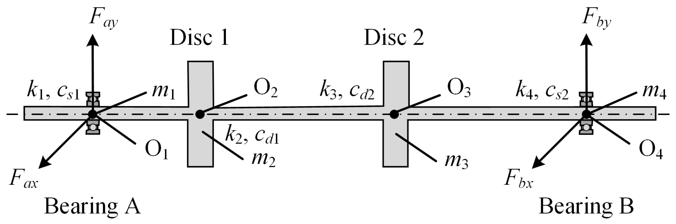
2.1. Preliminary
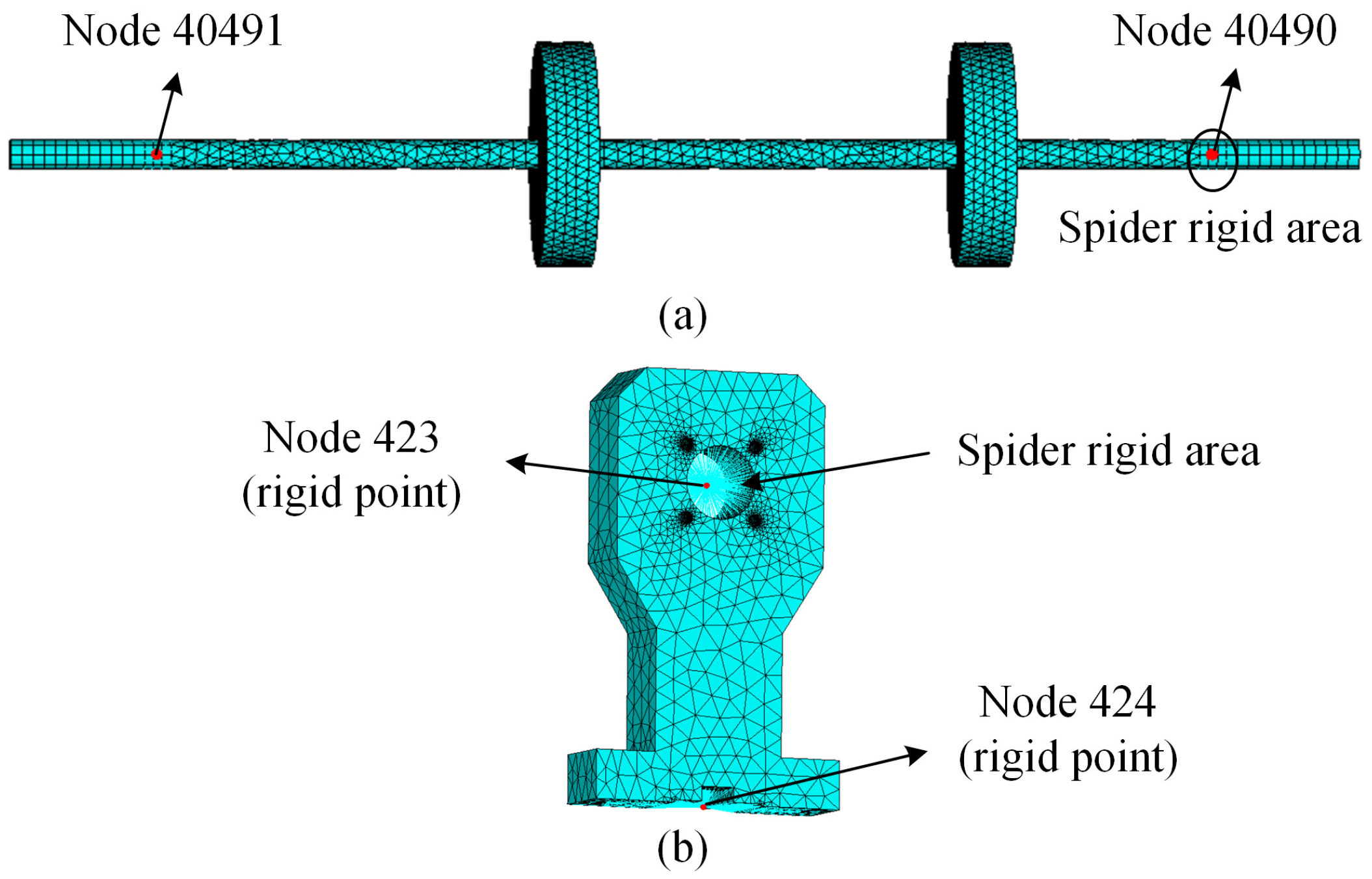
2.2. Numerical Simulation Implementation Using Physics-Based Model
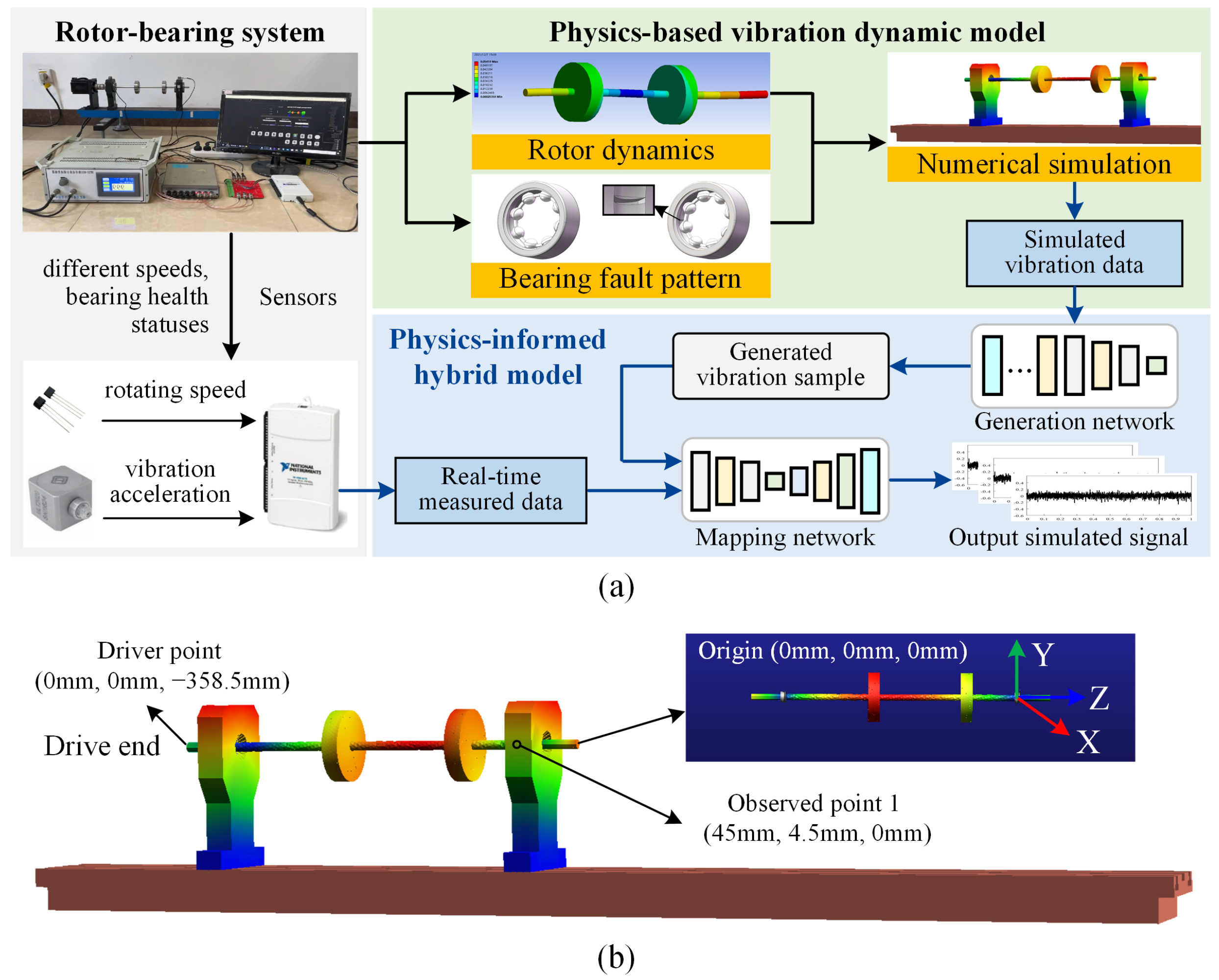
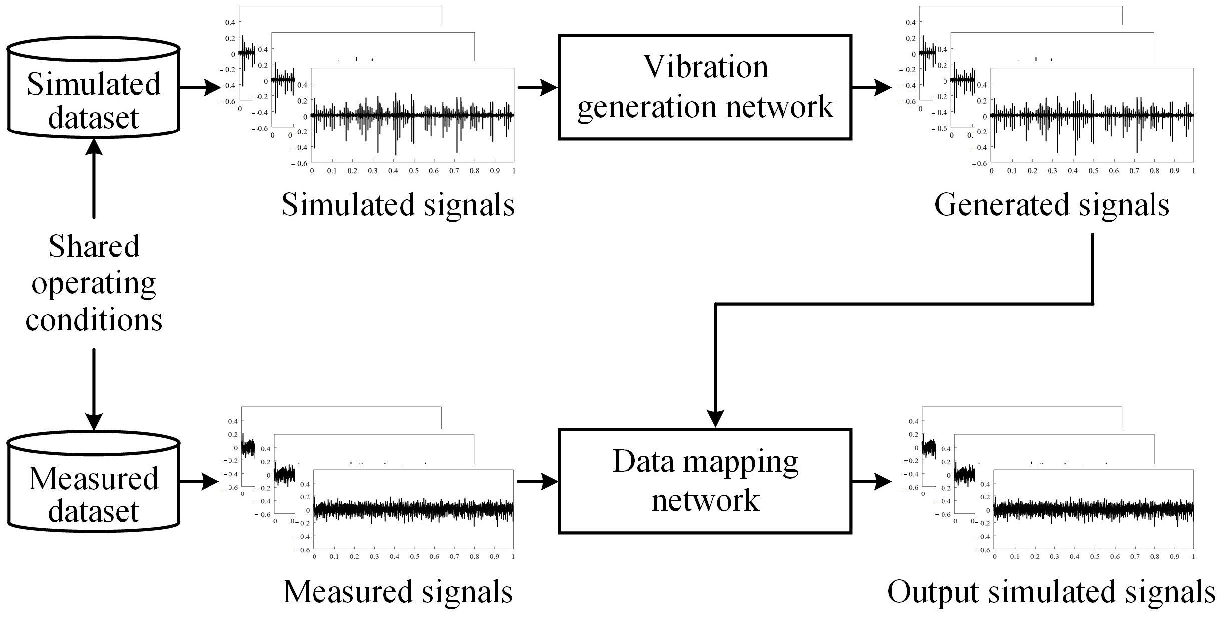
3. Physics-Informed Hybrid Modeling Method
3.1. Description of Simulated and Measured Vibration Datasets
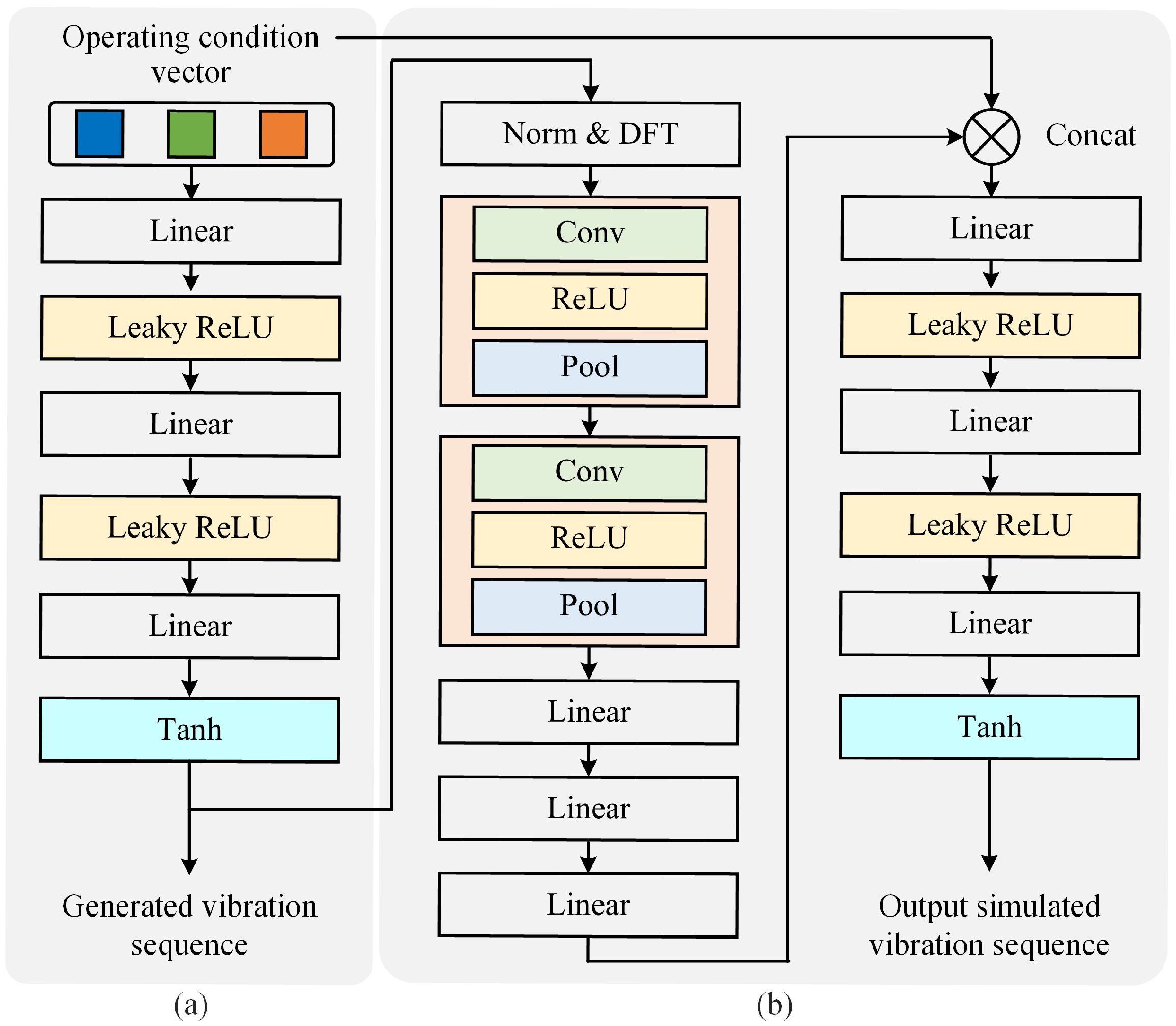
3.2. Construction of Vibration Generation Network
3.3. Construction of Data Mapping Network
4. Experimental Verification
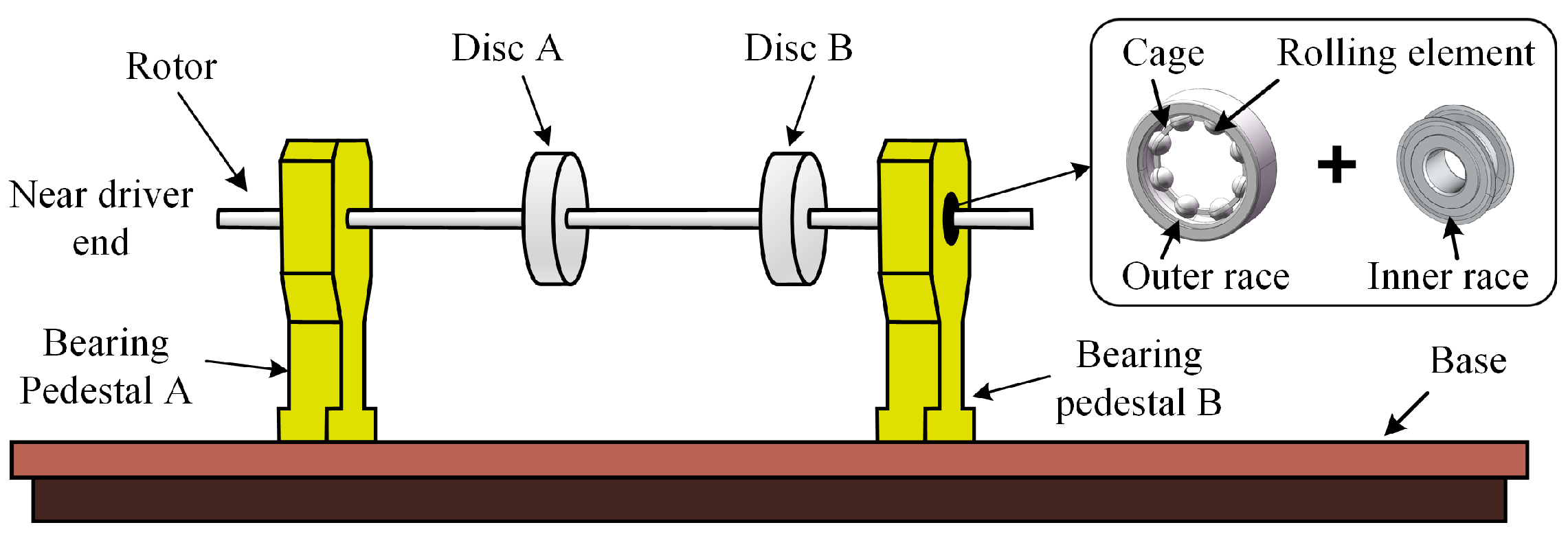
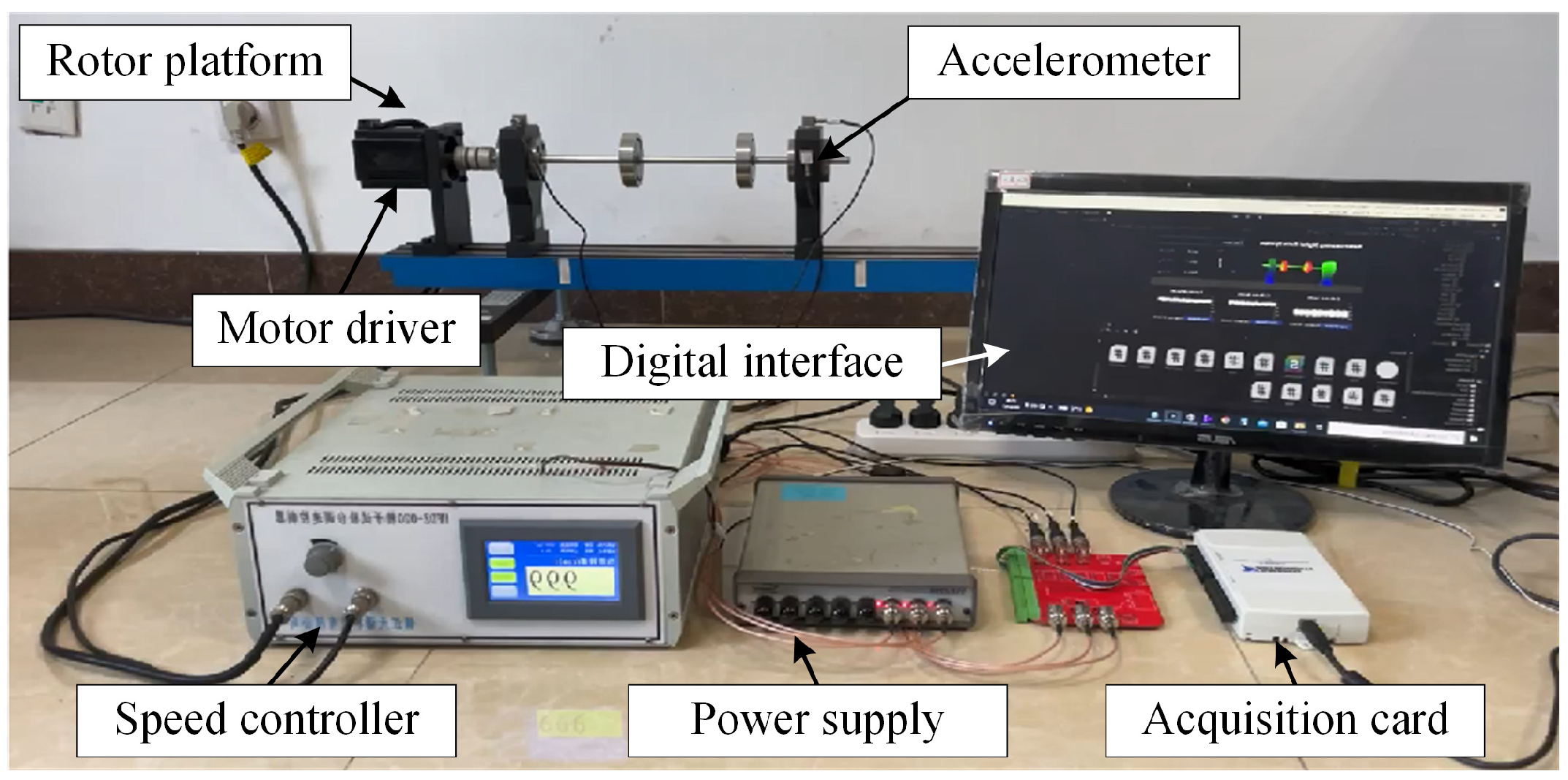
4.1. Experimental Setup
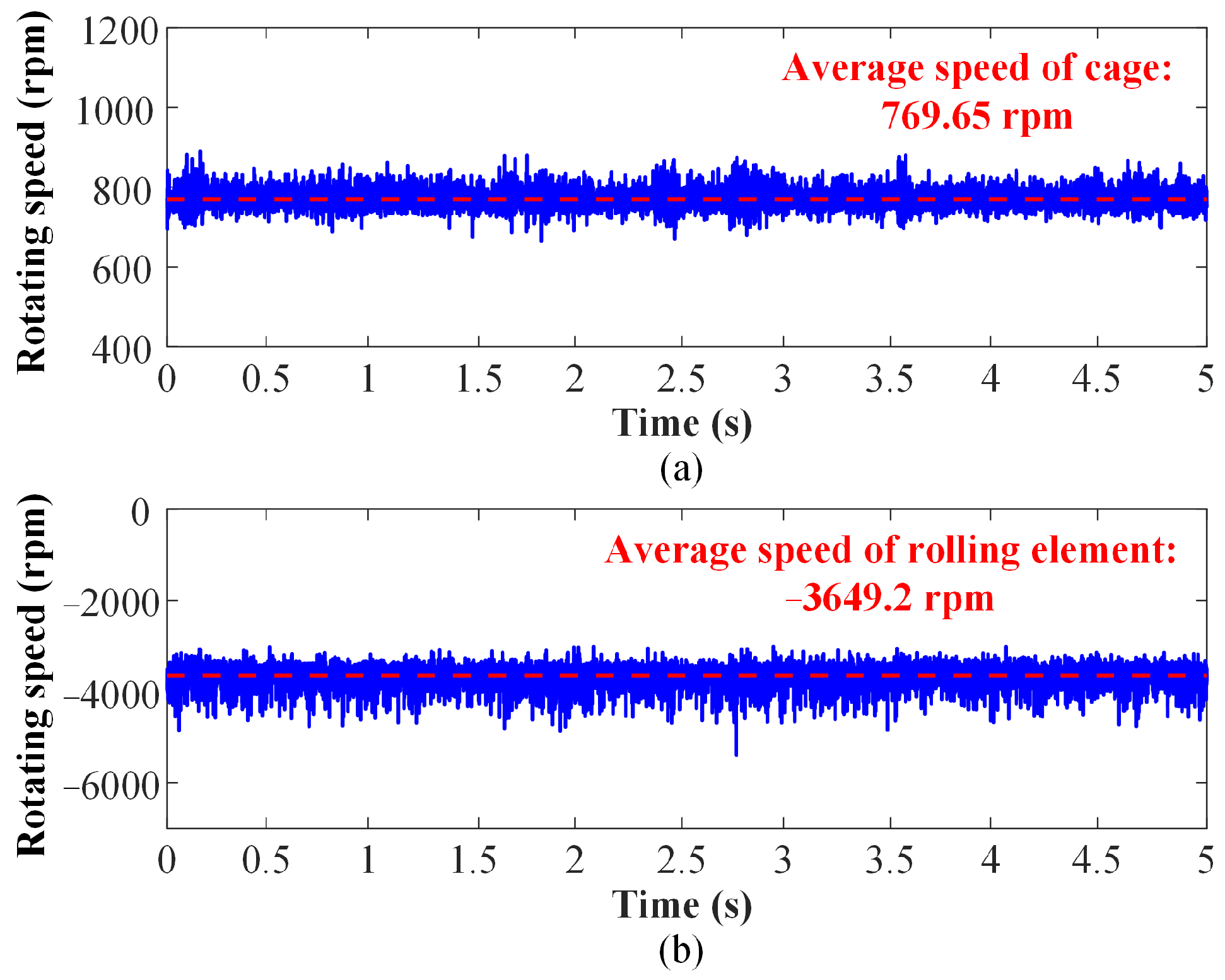
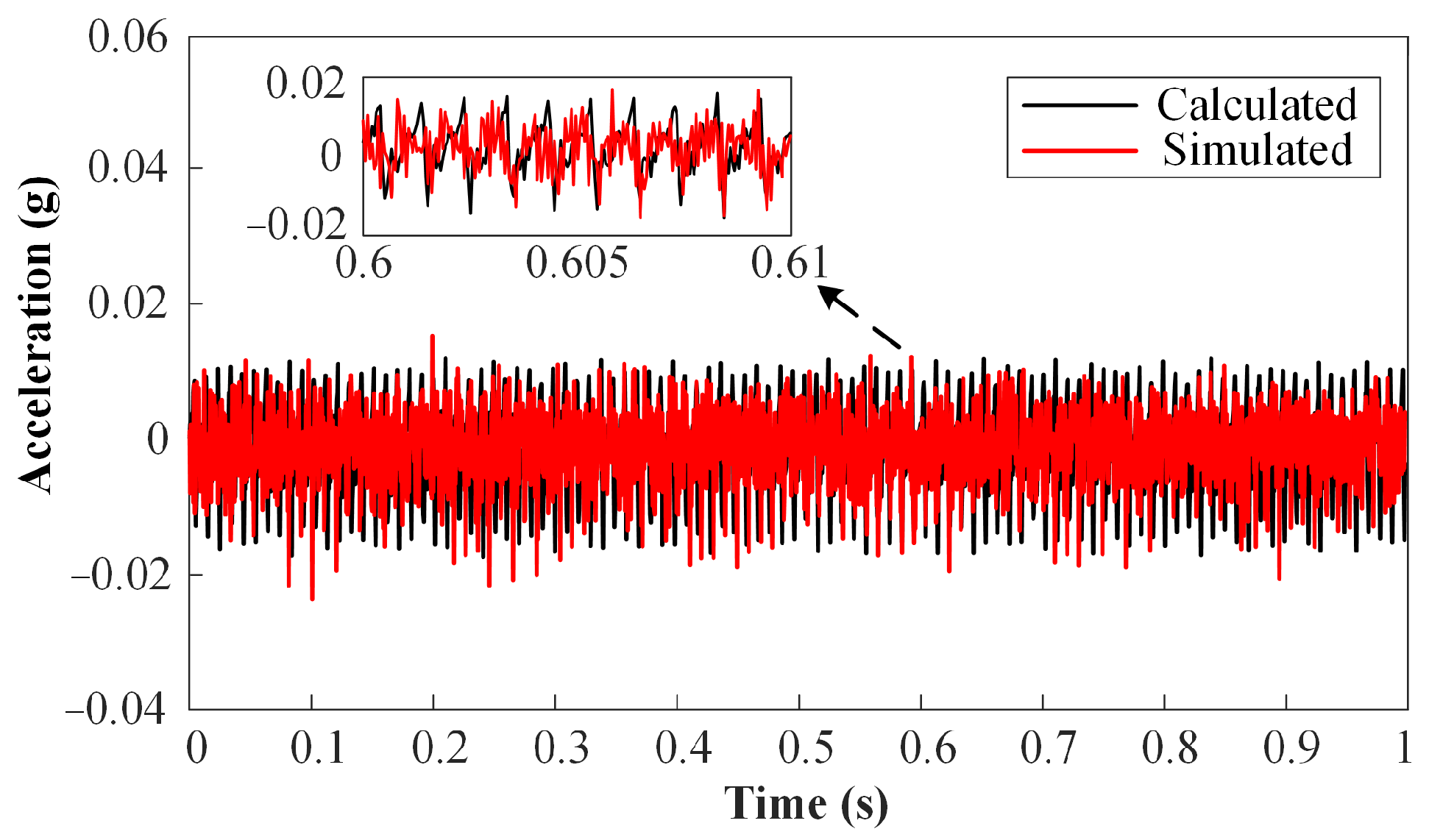
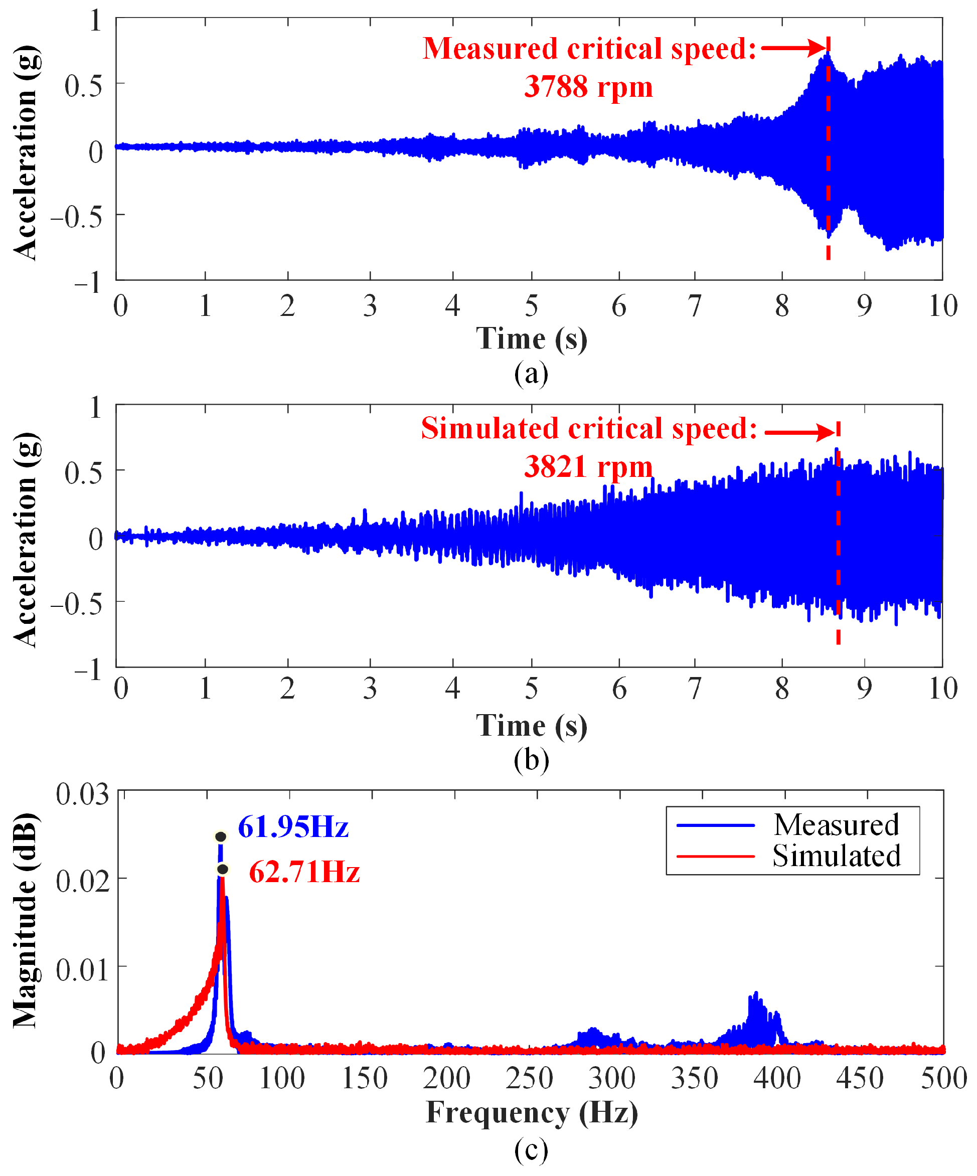
4.2. Numerical Analysis of Physics-Based Dynamic Vibration Model
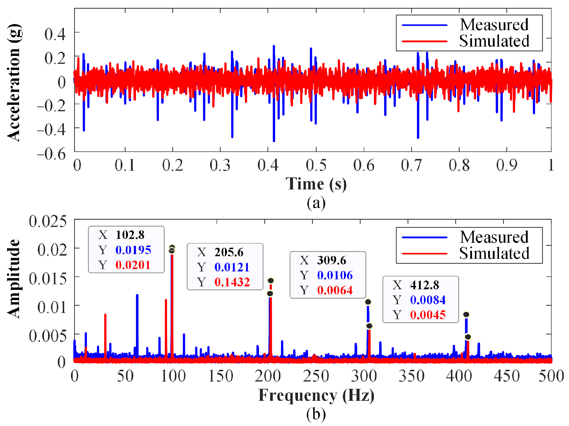
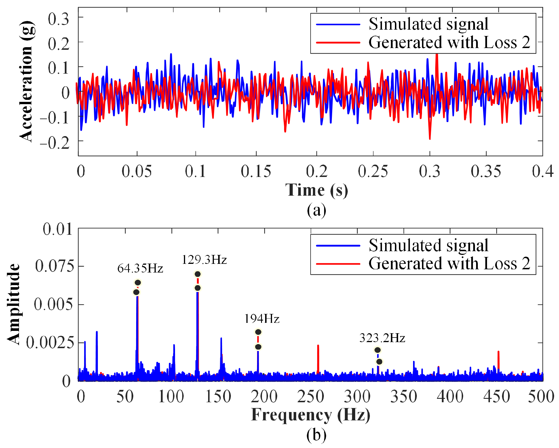
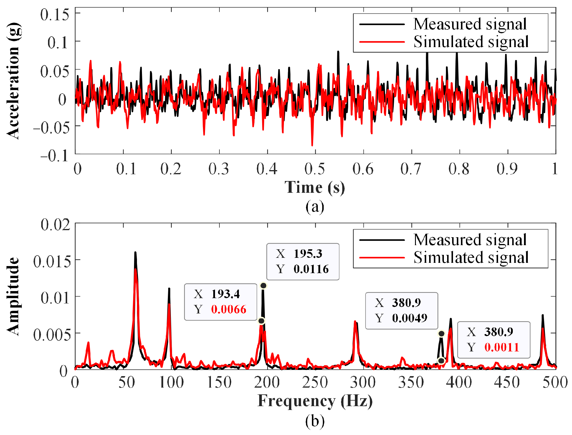
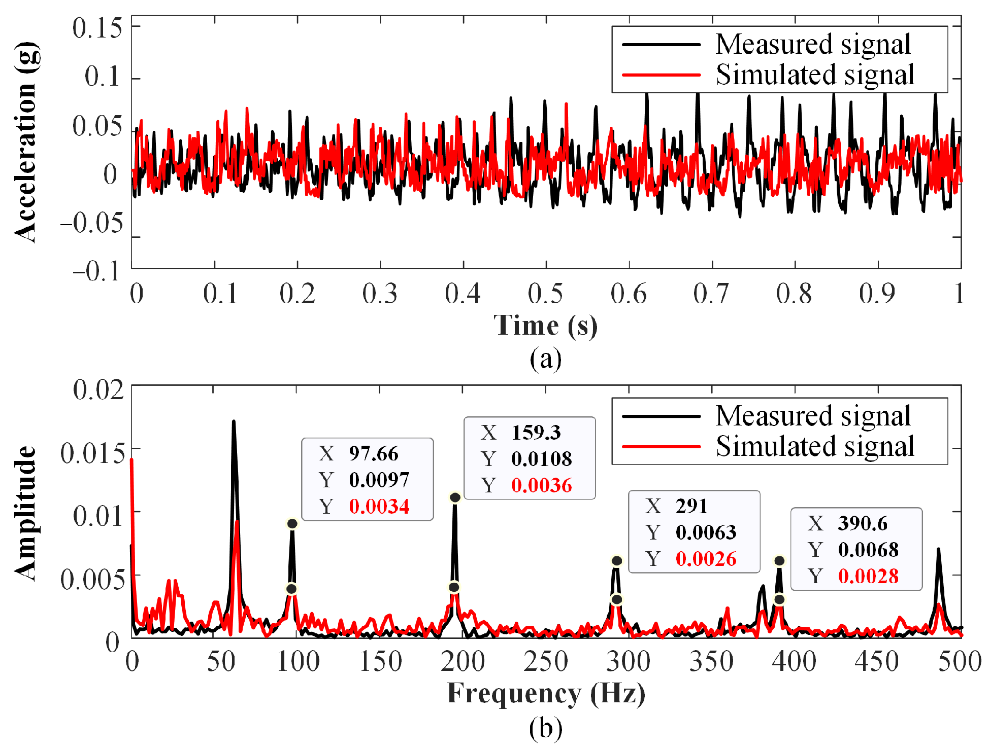
4.3. Generation of Simulated Vibration Samples and Their Validation
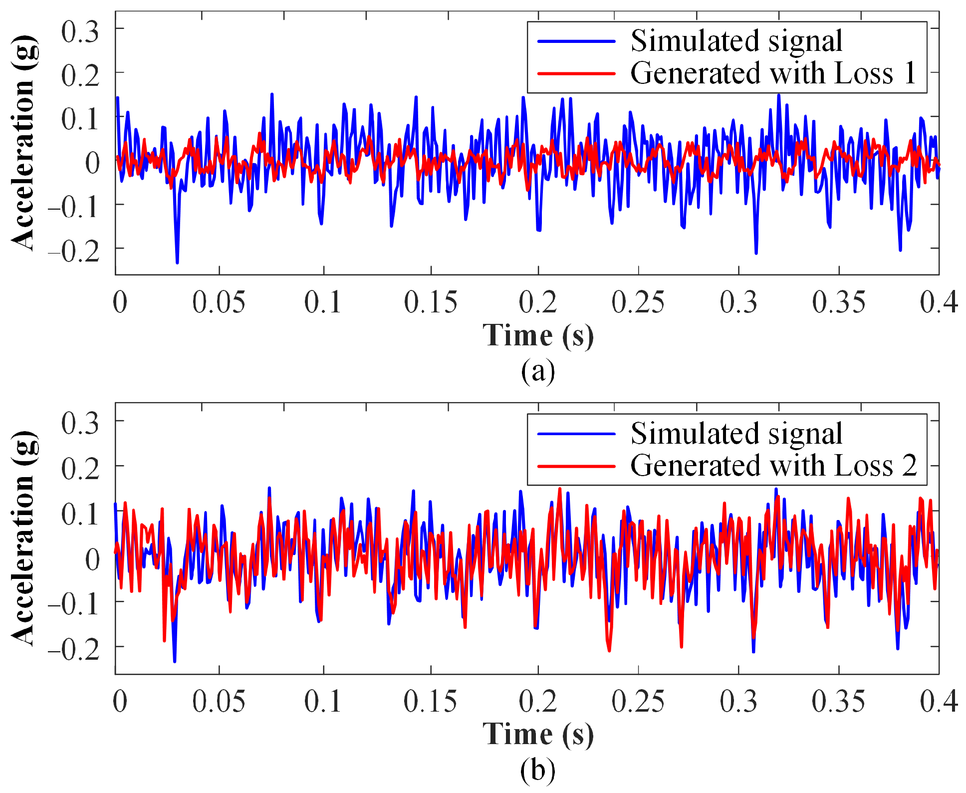
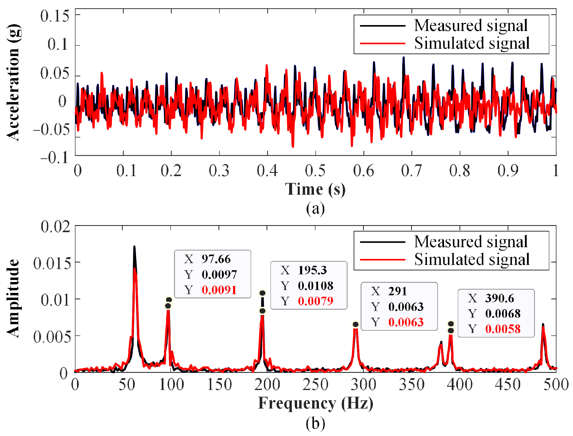
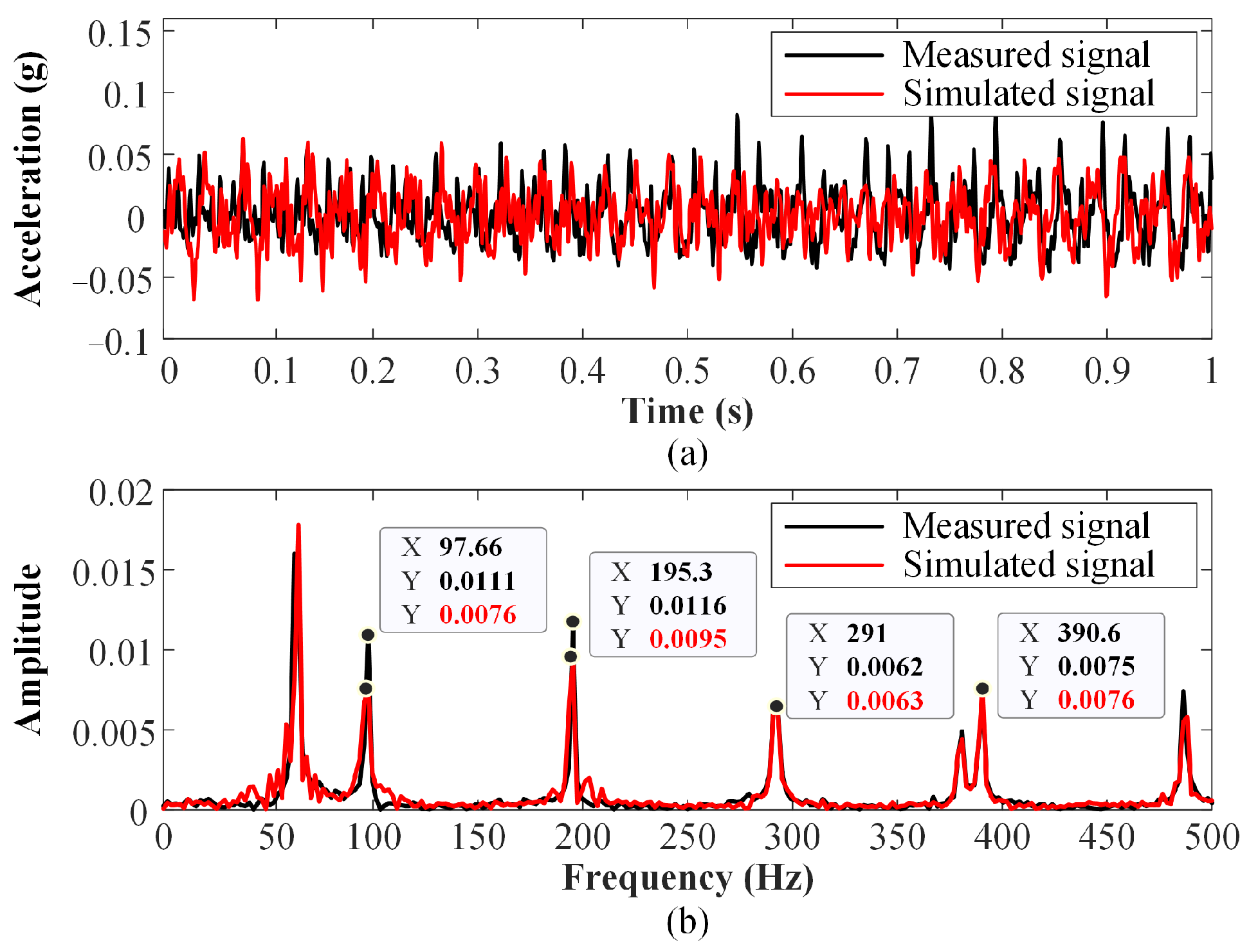
4.4. Performance Analysis of Physics-Informed Hybrid Modeling Method
5. Conclusions
Author Contributions
Funding
Data Availability Statement
Conflicts of Interest
Nomenclature
| , | equivalent masses of rotor at O and O |
| , | masses of discs |
| , | damping of rotor at O and O |
| , | damping of rotor at O and O |
| , , , | stiffness of rotor at O, O, O and O |
| g | acceleration due to gravity |
| , | supporting forces of bearing in radial x and y directions |
| Hertz elastic coefficient | |
| j | index of rolling elements |
| number of rolling elements | |
| rotating angular at time t of the jth rolling element | |
| contact deformation of the jth rolling element | |
| initial radial clearance of rolling bearing | |
| , | displacements of the inner race in radial x and y directions |
| , | displacements of the outer race in radial x and y directions |
| switching variable indicating the health status of the bearing | |
| displacement excitation caused by outer-race bearing fault | |
| initial angular of defect area | |
| span angular of defect area | |
| maximum value of the displacement excitation | |
| r | radius of rolling element |
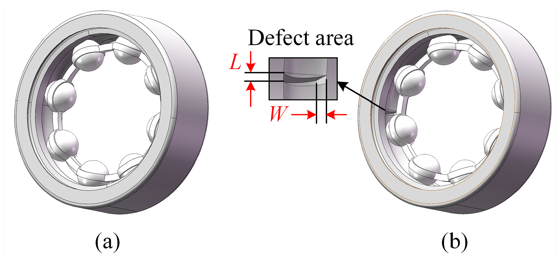
| L | length of defect area |
| stiffness coefficient of rolling bearing | |
| damping coefficient of rolling bearing | |
| preload of spring | |
| displacement caused by preload | |
| normal contact force | |
| d | penetration depth |
| force exponent | |
| K | equivalent contact stiffness |
| C | equivalent contact damping |
| distance from geometry center of the jth rolling element to raceway | |
| slip velocity | |
| coefficient of friction | |
| static coefficient of friction | |
| dynamic coefficient of friction | |
| static transition velocity | |
| dynamic transition velocity | |
| rotor angular speed | |
| W | width of defect area |
| optional weight coefficients | |
| T | discrete Fourier transform |
| rotating speed of cage | |
| rotating speed of rolling element | |
| center-circle radius of rolling element | |
| ratio of rolling element radius r to its center-circle radius | |
| rotating speed of bearing outer race | |
| fault characteristic frequency of outer-race fault |
References
- Zhu, W.; Lin, H.; Sun, W.; Wei, J. Vibration performance of traction gearbox of a high-speed train: Theoretical analysis and experiments. Actuators 2023, 12, 103. [Google Scholar] [CrossRef]
- Jafarian, M.; Nazarzadeh, J. Spectral analysis for diagnosis of bearing defects in induction machine drives. IET Electr. Power Appl. 2019, 13, 340–348. [Google Scholar] [CrossRef]
- Zhao, D.; Li, J.; Cheng, W.; Wen, W. Bearing multi-fault diagnosis with iterative generalized demodulation guided by enhanced rotational frequency matching under time-varying speed conditions. ISA Trans. 2023, 133, 518–528. [Google Scholar] [CrossRef] [PubMed]
- Zhu, D.; Gao, Q.; Sun, D.; Lu, Y. A detection method for bearing faults using complex-valued null space pursuit and 1.5-dimensional teager energy spectrum. IEEE Sens. J. 2020, 20, 8445–8454. [Google Scholar] [CrossRef]
- Rezamand, M.; Kordestani, M.; Orchard, M.E.; Carriveau, R.; Ting, D.S.K.; Saif, M. Improved remaining useful life estimation of wind turbine drivetrain bearings under varying operating conditions. IEEE Trans. Ind. Inform. 2020, 17, 1742–1752. [Google Scholar] [CrossRef]
- Wrzochal, M.; Adamczak, S. The problems of mathematical modelling of rolling bearing vibrations. Bull. Pol. Acad. Sci.-Tech. Sci. 2020, 68, 1363–1372. [Google Scholar]
- Singh, S.; Howard, C.; Hansen, C. An extensive review of vibration modelling of rolling element bearings with localised and extended defects. J. Sound Vibr. 2015, 357, 300–330. [Google Scholar] [CrossRef]
- McFadden, P.; Smith, J. Model for the vibration produced by a single point defect in a rolling element bearing. Bull. Pol. Acad. Sci.-Tech. Sci. 1984, 96, 69–82. [Google Scholar] [CrossRef]
- Su, Y.; Lin, S. On initial fault detection of a tapered roller bearing: Frequency domain analysis. J. Sound Vibr. 1992, 155, 75–84. [Google Scholar] [CrossRef]
- Liu, J. A dynamic modelling method of a rotor-roller bearing-housing system with a localized fault including the additional excitation zone. J. Sound Vibr. 2020, 469, 115144. [Google Scholar] [CrossRef]
- Wang, N.; Liu, M.; Yao, J.; Ge, P.; Wu, H. Numerical study on unbalance response of dual-rotor system based on nonlinear bearing characteristics of active magnetic bearings. Actuators 2023, 12, 86. [Google Scholar] [CrossRef]
- Li, Y.; Cao, H.; Niu, L.; Jin, X. A general method for the dynamic modeling of ball bearing-rotor systems. J. Manuf. Sci. Eng.-Trans. ASME 2015, 137, 021016. [Google Scholar] [CrossRef]
- Brouwer, M.; Sadeghi, F.; Ashtekar, A.; Archer, J.; Lancaster, C. Combined explicit finite and discrete element methods for rotor bearing dynamic modeling. Tribol. Trans. 2015, 58, 300–315. [Google Scholar] [CrossRef]
- Mishra, C.; Samantaray, A.K.; Chakraborty, G. Ball bearing defect models: A study of simulated and experimental fault signatures. J. Sound Vibr. 2017, 400, 86–112. [Google Scholar] [CrossRef]
- Liu, J.; Ni, H.; Li, X.; Xing, Q.; Pan, G. A simulation analysis of ball bearing lubrication characteristics considering the cage clearance. J. Tribol. 2023, 145, 044301. [Google Scholar] [CrossRef]
- Yu, Y.; Gao, H.; Zhou, S.; Pan, Y.; Zhang, K.; Liu, P.; Yang, H.; Zhao, Z.; Madyira, D.M. Rotor faults diagnosis in PMSMs based on branch current analysis and machine learning. Actuators 2023, 12, 145. [Google Scholar] [CrossRef]
- Popescu, T.; Aiordachioaie, D. Fault detection of rolling element bearings using optimal segmentation of vibrating signals. Mech. Syst. Signal Proc. 2019, 116, 370–391. [Google Scholar] [CrossRef]
- Yan, T.; Wang, D.; Xia, T.; Xi, L. A generic framework for degradation modeling based on fusion of spectrum amplitudes. IEEE Trans. Autom. Sci. Eng. 2020, 19, 308–319. [Google Scholar] [CrossRef]
- Wang, Y.; Yang, M.; Li, Y.; Xu, Z.; Wang, J.; Fang, X. A multi-input and multi-task convolutional neural network for fault diagnosis based on bearing vibration signal. IEEE Sens. J. 2021, 21, 10946–10956. [Google Scholar] [CrossRef]
- Wang, H.; Li, C.; Du, W. Coupled hidden Markov fusion of multichannel fast spectral coherence features for intelligent fault diagnosis of rolling element bearings. IEEE Trans. Instrum. Meas. 2021, 70, 1–10. [Google Scholar] [CrossRef]
- Shao, S.; Wang, P.; Yan, R. Generative adversarial networks for data augmentation in machine fault diagnosis. Comput. Ind. 2019, 106, 85–93. [Google Scholar] [CrossRef]
- Zhou, Q.; Hu, Y.; Liu, J. A novel assessable data augmentation method for mechanical fault diagnosis under noisy labels. Measurement 2022, 198, 111114. [Google Scholar]
- Liu, S.; Jiang, H.; Wu, Z.; Li, X. Data synthesis using deep feature enhanced generative adversarial networks for rolling bearing imbalanced fault diagnosis. Mech. Syst. Signal Proc. 2022, 163, 108139. [Google Scholar] [CrossRef]
- Jeong, H.; Bai, J.; Batuwatta-Gamage, C.P.; Rathnayaka, C.; Zhou, Y.; Gu, Y. A physics-informed neural network-based topology optimization (PINNTO) framework for structural Optimization. Eng. Struct. 2023, 278, 115484. [Google Scholar] [CrossRef]
- Chaiprabha, K.; Chancharoen, R. A deep trajectory controller for a mechanical linear stage using digital twin concept. Actuators 2023, 12, 91. [Google Scholar] [CrossRef]
- Li, L.; Li, Y.; Du, Q.; Liu, T.; Xie, Y. ReF-nets: Physics-informed neural network for Reynolds equation of gas bearing. Comput. Meth. Appl. Mech. Eng. 2022, 391, 115484. [Google Scholar] [CrossRef]
- Thelen, A.; Zhang, X.; Fink, O.; Lu, Y.; Ghosh, S.; Youn, B.D.; Todd, M.D.; Mahadevan, S.; Hu, C.; Hu, Z. A comprehensive review of digital twin—Part 1: Modeling and twinning enabling technologies. Struct. Multidiscip. Optim. 2022, 65, 354. [Google Scholar] [CrossRef]
- Lai, X.; Wang, S.; Guo, Z.; Zhang, C.; Sun, W.; Song, X. Designing a shape-performance integrated digital twin based on multiple models and dynamic data: A boom crane example. J. Mech. Des. 2021, 143, 071703. [Google Scholar] [CrossRef]
- Piltan, F.; Kim, J. Crack size identification for bearings using an adaptive digital twinn. Sensors 2021, 21, 5009. [Google Scholar] [CrossRef]
- Qin, Y.; Wu, X.; Luo, J. Data-model combined driven digital twin of life-cycle rolling bearing. IEEE Trans. Ind. Inform. 2021, 18, 1530–1540. [Google Scholar] [CrossRef]
- Wang, J.; Ye, L.; Gao, R.X.; Li, C.; Zhang, L. Digital Twin for rotating machinery fault diagnosis in smart manufacturing. Int. J. Prod. Res. 2019, 57, 3920–3934. [Google Scholar] [CrossRef]
- MSC ADAMS Reference Manual; MSC Software Corp.: Newport Beach, CA, USA, 2012; Available online: https://www.mscsoftware.com/product/adams (accessed on 21 February 2017).
- Giesbers, J. Contact Mechanics in MSC Adams—A Technical Evaluation of the Contact Models in Multibody Dynamics Software MSC Adams. Bachelor’s Thesis, University of Twente, Enschede, The Netherlands, 2012. [Google Scholar]
- Tu, W.; Liang, J.; Yu, W.; Shi, Z.; Liu, C. Motion stability analysis of cage of rolling bearing under the variable-speed condition. Nonlinear Dyn. 2023, 111, 11045–11063. [Google Scholar] [CrossRef]


| 1st Body | 2nd Body | Constraint Type |
|---|---|---|
| Base | Ground | Fixed joint |
| Bearing pedestal | Base | Spring-damping |
| Outer race | Bearing pedestal | Fixed joint |
| Inner race | Rotor | Fixed joint |
| Rolling element | Outer race, inner race | Contact force |
| Rolling element | Cage | Spherical joint |
| Parameter Type | Parameter | Value |
|---|---|---|
| Opecrating conditions | Rotor angular speed (/rpm) | 1000–2000 |
| Bearing health status () | 0, 1 | |
| Process-dependent parameters | Width of defect area (W/mm) | 1 |
| Length of defect area (L/mm) | 0.5 | |
| Observed Cartesian generalized coordinates (mm) | (45, 4.5, 0) | |
| Simulation parameters | Length per sample (s) | 1 |
| Step size per sample | 1/2000 |
| Network Layer | Output Size | Operator |
|---|---|---|
| Linear1 | 11 × 1 × 128 | Leaky_ReLU |
| Linear2 | 11 × 1 × 256 | Leaky_ReLU |
| Linear3 | 11 × 1 × 512 | Leaky_ReLU |
| Linear4 | 11 × 1 × 1000 | Tanh |
| Module | Network Layer | Output Size | Operator |
|---|---|---|---|
| Encoder | Conv1 | 11 × 3 × 501 | ReLU, MaxPool |
| Conv2 | 11 × 6 × 249 | ReLU, MaxPool | |
| Linear1 | 11 × 512 | ReLU | |
| Linear2 | 11 × 256 | ReLU | |
| Linear3 | 11 × 10 | – | |
| Decoder | Linear4 | 11 × 128 | Leaky_ReLU |
| Linear5 | 11 × 256 | Leaky_ReLU | |
| Linear6 | 11 × 512 | Leaky_ReLU | |
| Linear7 | 11 × 1000 | Tanh |
| Parameter | Numerical Value |
|---|---|
| Length of shaft (mm) | 460 |
| Radius of shaft (mm) | 5 |
| Radius of disc (mm) | 38 |
| Thickness of disc (mm) | 18 |
| Diameter of rolling element (mm) | 4.76 |
| Diameter of inner race (mm) | 10 |
| Diameter of outer race (mm) | 30 |
| Number of rolling elements | 8 |
| Contact angle () | 49.3 |
| Operating Condition | Dataset | Rotating Speed (rpm) | Number of Samples |
|---|---|---|---|
| Constant-speed | Simulated dataset | 1900 | 120 |
| Measured dataset | 1900 | 120 | |
| Variable-speed | Simulated dataset | 1800 1900 2000 | 120 120 120 |
| Measured dataset | 1800 1900 2000 | 120 10 120 |
Disclaimer/Publisher’s Note: The statements, opinions and data contained in all publications are solely those of the individual author(s) and contributor(s) and not of MDPI and/or the editor(s). MDPI and/or the editor(s) disclaim responsibility for any injury to people or property resulting from any ideas, methods, instructions or products referred to in the content. |
© 2023 by the authors. Licensee MDPI, Basel, Switzerland. This article is an open access article distributed under the terms and conditions of the Creative Commons Attribution (CC BY) license (https://creativecommons.org/licenses/by/4.0/).
Share and Cite
Zhu, M.; Peng, C.; Yang, B.; Wang, Y. A Novel Physics-Informed Hybrid Modeling Method for Dynamic Vibration Response Simulation of Rotor–Bearing System. Actuators 2023, 12, 460. https://doi.org/10.3390/act12120460
Zhu M, Peng C, Yang B, Wang Y. A Novel Physics-Informed Hybrid Modeling Method for Dynamic Vibration Response Simulation of Rotor–Bearing System. Actuators. 2023; 12(12):460. https://doi.org/10.3390/act12120460
Chicago/Turabian StyleZhu, Mengting, Cong Peng, Bingyun Yang, and Yu Wang. 2023. "A Novel Physics-Informed Hybrid Modeling Method for Dynamic Vibration Response Simulation of Rotor–Bearing System" Actuators 12, no. 12: 460. https://doi.org/10.3390/act12120460
APA StyleZhu, M., Peng, C., Yang, B., & Wang, Y. (2023). A Novel Physics-Informed Hybrid Modeling Method for Dynamic Vibration Response Simulation of Rotor–Bearing System. Actuators, 12(12), 460. https://doi.org/10.3390/act12120460