Model-Independent Observer-Based Current Sensorless Speed Servo Systems with Adaptive Feedback Gain

Abstract

This study proposes a solution to the speed control problem of servo machines in the form of multi-loop current sensorless control with a reduction in the system model dependence level and the number of feedback loops, which provides the two contributions: first, a model-independent observer estimates speed and acceleration using only the position measurement, thereby ensuring the first-order estimation error dynamics; second, the active damping acceleration stabilizes the inner loop with the adaptive feedback gain increasing and decreasing automatically according to the transient and steady-state operation modes. The experimental study highlighted the effectiveness of the acceleration loop adaptation technique, which used an actual servo system comprising the QUBE-servo2 and myRIO-1900.

1. Introduction

Industrial machines that need high accuracy (such as conveyor belts, roll-to-rolls and electric vehicles) require their servo systems to increase their reliability and power efficiency under severe and uncertain operating conditions. These concerns can be addressed by the engineering in software and hardware layers. Fortunately, it has been reported that the closed-loop performance of servo systems significantly depends on the embedded system engineering (software layer) [1,2,3,4,5,6].

The multi-loop feedback system structure that contains a current controller (as the inner loop) and a speed controller (as the outer loop) has been widely adopted as the soft layer of speed servo system applications. Their hardware layers have been implemented using a (single-phase) DC motor or (three-phase) brushless DC, permanent magnet synchronous and induction motors, according to the output power specifications [7]. Proportional–integral (PI) regulators have mainly been implemented in each loop through the error signal feedback that is weighted by the gain and treated as the tuning factor. The desired specifications for each loop are provided by the cut-off frequency from the reference and output (current and speed) signals and the PI gains satisfy these requirements by applying Bode and Nyquist plots (frequency domain design techniques) [8,9]. However, servo system parameters and load uncertainties limit the resulting closed-loop performance, which can be addressed by the gain scheduler involving online membership tests [10]. Additionally, the signal error of the speed sensor or the speed control of the servo motor problems may be solved by the use of a speedless sensing solution [11].

As a nonlinear approach, an integral back-stepping controller that forms part of the multi-loop structure can yield the current and voltage commands for each loop, including the parameter-dependent feedback gains of the system and the feed-forward compensator, which cancels the open-loop zero to render the first-order current and speed transfer function to the closed-loop [12]. These novel online parameter estimation techniques can help to alleviate the parameter dependence levels of the system by increasing computational complexity and the number of tuning factors [13,14,15]. Optimal adaptive controllers that directly handle model–plant mismatches have been be considered as alternatives [16,17,18]. An online auto-tuning mechanism has been presented as a subsystem for the adaptive back-stepping controller to boost the feedback gain during transient periods; however, the increased feedback gain value has raised concerns regarding a reduction in stability margins [17]. The recently developed disturbance observer (DOB)-based controller has adopted an energy-shaping technique that addresses this concern by incorporating the damping terms into the auto-tuning system [19,20]. The DOB controller depends on system parameters improving the closed-loop performance by producing the state and disturbance estimates that are used for the nonlinear control actions [21]. A nonlinear DOB-based multi-loop passive damping controller has solved these system parameter dependence problems, thereby ensuring performance recovery properties by analyzing the closed-loop dynamics using the Lyapunov analysis technique [22]. A sliding mode controller into which a nonlinear DOB was embedded has achieved the finite convergence time of the desired performance by reducing the steady-state chattering level; however, the discontinuous feedback loop was still maintained [23]. The finite control set model predictive controls (FCSMPCs) select the optimal current and voltage commands for the performance of each loop by involving online membership tests and predicting the behavior of the current and speed using a mathematical model of the servo system [24,25].

From the aforementioned literature survey, practical challenges are identified, such as (a) the model dependence levels of the control and the observer and (b) the high gain of the inner loop. The proposed solution forms a multi-loop structure to solve these practical problems and presents the following contributions:

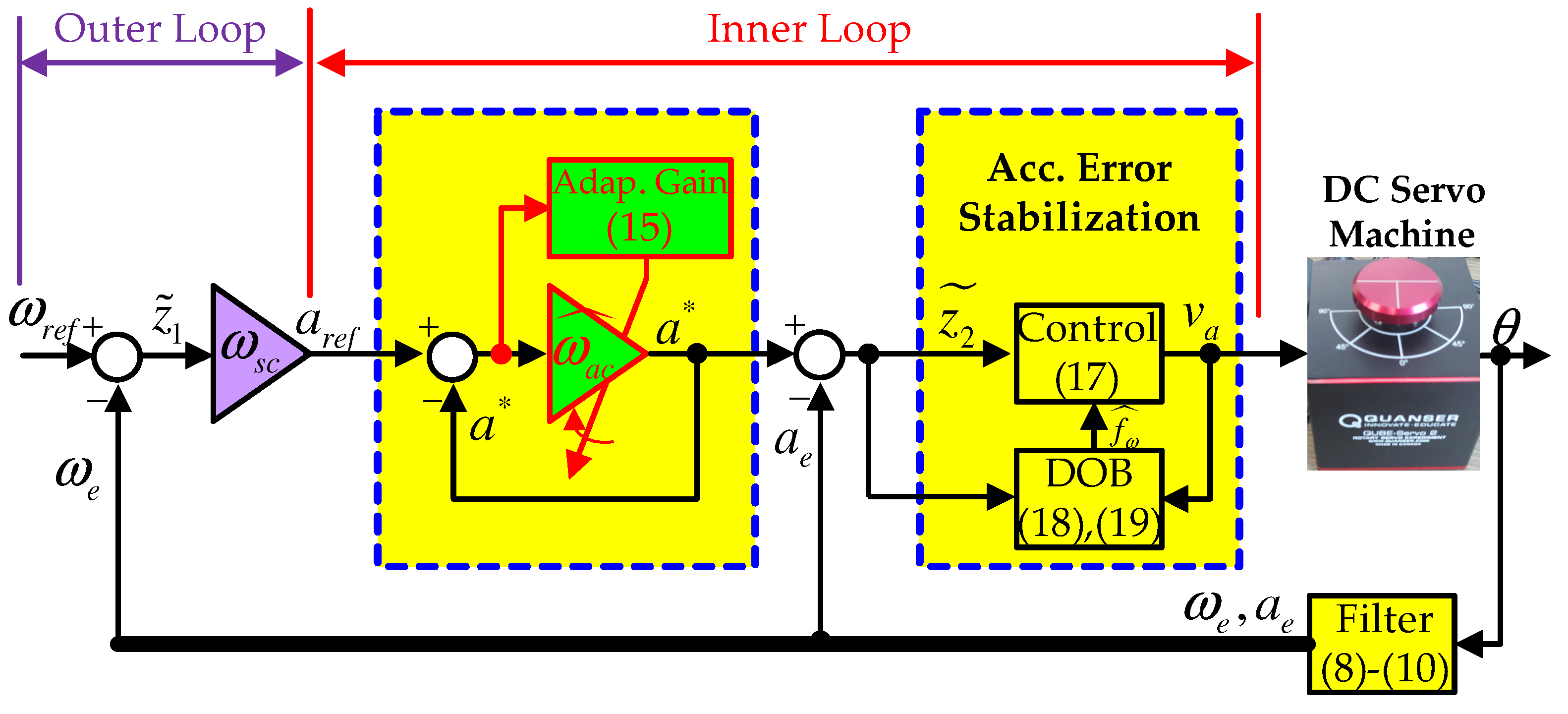
• For the entire loop, the observer gain is obtained by allowing each control loop, without addressing the matrix algebra using a model-independent observer, to estimate speed and acceleration as the pivotal subsystems;
• For the inner loop, the robust acceleration error stabilization loop is driven by the active damping, according to the first-order dynamics, which leads to the pole-zero cancellation;
• For the inner loop, the adaptive acceleration feedback gain is governed by the analytic law with the nonlinear excitation term of the acceleration error, thereby boosting and reducing its value according to the transient and steady-state operations.

The actual performance improvement of the proposed solution in terms of these contributions is validated using experimental studies on servo systems that consisted of QUBE-servo2 (hardware) and myRIO-1900 (software).

2. Servo Machine Dynamics

The electrical and mechanical motions of three-phase servo machines (permanent magnet synchronous and induction motors) can be expressed similarly to the DC servo machine by applying the time-varying coordinate transform that is synchronized to the machine position [26]. Thus, this study considers the DC servo machine to be the simplest case to demonstrate the main idea of this work. The system dynamics are described as a third-order linear system that is perturbed by a mismatched disturbance from the load torque $T_L\left(t\right)$ (in Nm):

$$\begin{array}{ccc}\hfill \frac{d\theta \left(t\right)}{dt}& =& \omega \left(t\right),\hfill \end{array}$$

(1)

$$\begin{array}{ccc}\hfill J\frac{d\omega \left(t\right)}{dt}& =& -B\omega \left(t\right)+T_e\left(i_a\left(t\right)\right)-T_L\left(t\right),\hfill \end{array}$$

(2)

$$\begin{array}{ccc}\hfill L\frac{d{i}_a\left(t\right)}{dt}& =& -R{i}_a\left(t\right)-k_e\omega \left(t\right)+v_a\left(t\right),\forall t\ge 0,\hfill \end{array}$$

(3)

where the armature voltage $v_a\left(t\right)$ (in V) excites the armature current $i_a\left(t\right)$ (in A), the electrical torque $T_e\left(i_a\left(t\right)\right)=k_T{i}_a\left(t\right)$ (in Nm) with coefficient $k_T>0$, the rotational speed $\omega \left(t\right)$ (in rad/s), and the position $\theta \left(t\right)$ (in rad), sequentially. The rotor inertia J (in kgm²), viscous friction B (in Nm/rad/s), armature inductance L (in H), armature resistance R (in $\Omega$) and back electromotive force coefficient $k_e$ characterizes the actual dynamics of servo machines, which involve uncertainties depending on the operating conditions, such as $J=J_0+\Delta J$ with a known nominal value $J_0$ (provided by the manufacturer) and unknown variation $\Delta J$.

A system parameter decomposition such that $(·)={(·)}_0+\Delta (·)$ simplifies the dynamic relationship between the armature voltage $v_a\left(t\right)$ and the speed $\omega \left(t\right)$ using the original dynamics in (2) and (3) as:

$$\begin{array}{c}\hfill c_{\omega ,0}\frac{d^2\omega \left(t\right)}{d{t}^2}=v_a\left(t\right)+{\overline{f}}_{\omega }\left(t\right),\forall t\ge 0,\end{array}$$

(4)

where the known coefficient $c_{\omega ,0}:=\frac{J_0{L}_0}{k_{T,0}}>0$ and the unknown time-varying lumped disturbance ${\overline{f}}_{\omega }\left(t\right):=-R{i}_a\left(t\right)-k_e\omega \left(t\right)-\frac{BL}{k_T}\frac{d\omega \left(t\right)}{dt}-\frac{d{T}_L\left(t\right)}{dt}+(\frac{J_0{L}_0}{k_{T,0}}-\frac{JL}{k_T})\frac{d^2\omega \left(t\right)}{d{t}^2}$, which not only reduces the model dependence of the control algorithm compared to the use of the original dynamics in (2) and (3) but also eliminates the requirement for the current feedback. The following sections present the observer-based speed control law that is based on the second-order open-loop dynamics (4) and analyze the resulting feedback system using the notation $\dot{f}\left(t\right):=\frac{df\left(t\right)}{dt}$ for any differentiable functions $f\left(t\right)$, $\forall t\ge 0$.

3. Proposed Solution

The two signals ${\omega }^{*}\left(t\right)$ and ${\omega }_{ref}\left(t\right)$ are defined as the desired closed-loop speed trajectory and reference signal with their Laplace transforms ${\Omega }^{*}\left(s\right)$ and ${\Omega }_{ref}\left(s\right)$, respectively. This study defines the target closed-loop performance in the low-pass filter form, which is given as:

$$\begin{array}{c}\hfill \frac{{\Omega }^{*}\left(s\right)}{{\Omega }_{ref}\left(s\right)}=\frac{{\omega }_{sc}}{s+{\omega }_{sc}},\forall s\in \mathbb{C},\end{array}$$

(5)

where the tracking performance ${\omega }_{sc}$ represents the cut-off frequency of the system (5) in rad/s (e.g., $f_{sc}=\frac{{\omega }_{sc}}{2\pi }$ Hz). The application of inverse Laplace transform to (5) yields

$$\begin{array}{c}\hfill {\dot{\omega }}^{*}\left(t\right)={\omega }_{sc}({\omega }_{ref}\left(t\right)-{\omega }^{*}\left(t\right)),\forall t\ge 0,\end{array}$$

(6)

defining the control objective as the exponential convergence

$$\begin{array}{c}\hfill \underset{t\to \infty }{lim}\omega \left(t\right)={\omega }^{*}\left(t\right)\end{array}$$

(7)

to assign the target transfer function (5) to the closed-loop, incorporating the adaptive feedback gain into the inner loop, thus stabilizing the acceleration error.

3.1. Model-Independent Observer

The speed $\omega \left(t\right)$ could be estimated using the servo system models in (1) and (2) by applying the Luenberger observer design technique, depending on the machine parameter information, as could the acceleration $a\left(t\right)$ using the models in (1)–(3). The model dependence could degrade not only the accuracy of the speed and acceleration estimation but also the transient performance, which is a main challenge of this subsection.

Regarding the observer output ${\theta }_e\left(t\right)$ with its error $e_{\theta }\left(t\right):=\theta \left(t\right)-{\theta }_e\left(t\right)$, the speed and acceleration estimates are defined as ${\omega }_e\left(t\right)$ and $a_e\left(t\right)$ for their actual measurements, with $\omega \left(t\right)(=\dot{\theta }\left(t\right))$ and $a\left(t\right)(=\dot{\omega }\left(t\right))$ leading to the estimation errors $e_{\omega }\left(t\right):=\omega \left(t\right)-{\omega }_e\left(t\right)$ and $e_a\left(t\right):=a\left(t\right)-a_e\left(t\right)$, and the augmented observer error is defined as ${\mathbf{e}}_{\theta }:={\left[\begin{array}{ccc}{e}_{\theta }\left(t\right)& e_{\omega }\left(t\right)& e_a\left(t\right)\end{array}\right]}^T$. Based on these notations, this subsection presents the proposed observer:

$$\begin{array}{ccc}\hfill {\dot{\theta }}_e\left(t\right)& =& (2k_{d,e}+{\lambda }_e)e_{\theta }\left(t\right)+{\omega }_e\left(t\right),\hfill \end{array}$$

(8)

$$\begin{array}{ccc}\hfill {\dot{\omega }}_e\left(t\right)& =& (k_{d,e}^2+2{\lambda }_e{k}_{d,e})e_{\theta }\left(t\right)+a_e\left(t\right),\hfill \end{array}$$

(9)

$$\begin{array}{ccc}\hfill {\dot{a}}_e\left(t\right)& =& k_{d,e}^2{\lambda }_e{e}_{\theta }\left(t\right),\forall t\ge 0,\hfill \end{array}$$

(10)

where the two tuning parameters $k_{d,e}>0$ and ${\lambda }_e>0$ define the gains for each subsystem such that $l_1:=2k_{d,e}+{\lambda }_e$ (for (8)), $l_2:=k_{d,e}^2+2{\lambda }_e{k}_{d,e}$ (for (9)) and $l_3:=k_{d,e}^2{\lambda }_e$ (for (10)). The proposed observer comprising (8)–(10) requires no model information, including the structure and coefficient values, and it ensures the beneficial convergence property:

$$\begin{array}{c}\hfill \underset{t\to \infty }{lim}{e}_x\left(t\right)=e_x^{*}\left(t\right),x=\theta ,\omega ,a,\end{array}$$

exponentially for the desired output and estimation error trajectories that satisfies the desired system ${\dot{e}}_x^{*}\left(t\right)=-{\lambda }_e{e}_x^{*}\left(t\right)$ with $e_x^{*}\left(t\right):=x\left(t\right)-x_e^{*}\left(t\right)$, $x=\theta ,\omega ,a$, $\forall t\ge 0$, as shown in Section 4.

3.2. Outer Loop: Speed Control

The outer loop determines the desired acceleration reference signal $a_{ref}\left(t\right)$ according to the speed error ${\omega }_{ref}\left(t\right)-\omega \left(t\right)$. Consequently, the new variables are defined as $z_1\left(t\right):={\omega }_e\left(t\right)$ and $z_2\left(t\right):=a_e\left(t\right)$, which yields the dynamics using (8):

$$\begin{array}{ccc}\hfill {\dot{z}}_1\left(t\right)& =& l_2{e}_{\theta }\left(t\right)+a_e\left(t\right)\hfill \\ & =& a_{ref}\left(t\right)-\Delta z_2\left(t\right)+l_2{e}_{\theta }\left(t\right),\forall t\ge 0,\hfill \end{array}$$

(11)

where $a_{ref}\left(t\right)$ denotes the additional design variable and $\Delta z_2\left(t\right):=a_{ref}\left(t\right)-z_2\left(t\right)$. This study chooses to use the update rule for $a_{ref}\left(t\right)$ as the simple proportional feedback control:

$$\begin{array}{c}\hfill a_{ref}\left(t\right)={\omega }_{sc}{\tilde{z}}_1\left(t\right),\forall t\ge 0,\end{array}$$

(12)

with the error ${\tilde{z}}_1\left(t\right):={\omega }_{ref}\left(t\right)-z_1\left(t\right)$, which result in a controlled outer loop system by substituting (12) into the open-loop dynamics (11):

$$\begin{array}{c}\hfill {\dot{z}}_1\left(t\right)={\omega }_{sc}{\tilde{z}}_1\left(t\right)-\Delta z_2\left(t\right)+{\mathbf{c}}_1^T{\mathbf{e}}_{\theta }\left(t\right),\forall t\ge 0,\end{array}$$

(13)

where ${\mathbf{c}}_1:={\left[\begin{array}{ccc}{l}_2& 0& 0\end{array}\right]}^T$. See Section 4 for a further analysis of the controlled outer loop ${\omega }_{ref}\left(t\right)\mapsto \omega \left(t\right)$.

3.3. Inner Loop: Acceleration Error Stabilizer

The inner loop determines the desired commands for the armature voltage $v_a\left(t\right)$ according to the input signal $a_{ref}\left(t\right)$ from the outer loop (e.g., $a_{ref}\left(t\right)\mapsto v_a\left(t\right)$), which comprises two parts: a desired acceleration trajectory generator that was driven by the adaptive feedback gain (Section 3.3.1) and an error stabilizer (Section 3.3.2).

3.3.1. Desired Acceleration Trajectory Generator

For the input signal $a_{ref}\left(t\right)$ from the outer loop, the error ${\tilde{a}}^{*}\left(t\right):=a_{ref}\left(t\right)-a^{*}\left(t\right)$ is defined as driving the subsystem that generates the desired acceleration trajectory $a^{*}\left(t\right)$ such that

$$\begin{array}{c}\hfill {\dot{a}}^{*}\left(t\right)={\widehat{\omega }}_{ac}\left(t\right){\tilde{a}}^{*}\left(t\right),\forall t\ge 0,\end{array}$$

(14)

subject to the adaptive feedback gain ${\widehat{\omega }}_{ac}\left(t\right)$ that is updated by the rule:

$$\begin{array}{c}\hfill {\dot{\widehat{\omega }}}_{ac}\left(t\right)={\gamma }_{ac}({\left({\tilde{a}}^{*}\left(t\right)\right)}^2+{\rho }_{ac}{\tilde{\omega }}_{ac}\left(t\right)),\forall t\ge 0,\end{array}$$

(15)

where ${\tilde{\omega }}_{ac}\left(t\right):={\omega }_{ac}-{\widehat{\omega }}_{ac}\left(t\right)$ for some steady-state gains and ${\omega }_{ac}>0$, which initializes ${\widehat{\omega }}_{ac}\left(0\right)={\omega }_{ac}$. The first tuning parameter ${\gamma }_{ac}>0$ adjusts the excitation level of ${\widehat{\omega }}_{ac}\left(t\right)$ and the remaining ${\rho }_{ac}>0$ determines the decay ratio to the steady-state gain ${\omega }_{ac}$. The two subsystems of (14) and (15) constitute the input–output mapping $a_{ref}\left(t\right)\mapsto a^{*}\left(t\right)$ along the adaptive feedback gain ${\widehat{\omega }}_{ac}\left(t\right)$. Owing to the time-varying nature of the feedback gain ${\widehat{\omega }}_{ac}\left(t\right)$ for the subsystem in (14) and the nonlinear excitation term ${\left({\tilde{a}}^{*}\left(t\right)\right)}^2$ for the subsystem in (15), the stability issue of the system $a_{ref}\left(t\right)\mapsto a^{*}\left(t\right)$ remains questionable. See Section 4 for a further analysis.

3.3.2. Acceleration Error Stabilizing Control

For the input signal $a^{*}\left(t\right)$ from the subsystem in (14), the error ${\tilde{z}}_2\left(t\right):=a^{*}\left(t\right)-z_2\left(t\right)$ is defined as yielding the dynamics (using (4) and (10)):

$$\begin{array}{ccc}\hfill c_{\omega ,0}{\dot{\tilde{z}}}_2\left(t\right)& =& -c_{\omega ,0}{\dot{a}}_e\left(t\right)+c_{\omega ,0}{\dot{a}}^{*}\left(t\right)\hfill \\ & =& -v_a\left(t\right)+f_{\omega }\left(t\right)+c_{\omega ,0}{\dot{e}}_a\left(t\right),\forall t\ge 0,\hfill \end{array}$$

(16)

with the newly defined lumped disturbance $f_{\omega }\left(t\right):=c_{\omega ,0}{\dot{a}}^{*}\left(t\right)-{\overline{f}}_{\omega }\left(t\right)$, which is stabilized using the proposed active damping control:

$$\begin{array}{c}\hfill v_a\left(t\right)=(k_{d,ac}+c_{\omega ,0}{\lambda }_{ac}){\tilde{z}}_2\left(t\right)+k_{d,ac}{\lambda }_{ac}{\int }_0^t{\tilde{z}}_2\left(\tau \right)d\tau +{\widehat{f}}_{\omega }\left(t\right),\forall t\ge 0,\end{array}$$

(17)

with the two tuning parameters: active damping $k_{d,ac}>0$ and stabilization rate ${\lambda }_{ac}>0$. The DOB governs the dynamics of the feed-forward compensation term ${\widehat{f}}_{\omega }\left(t\right)$ as:

$$\begin{array}{ccc}\hfill {\dot{q}}_{\omega }\left(t\right)& =& -l_{\omega }{q}_{\omega }\left(t\right)-l_{\omega }^2{c}_{\omega ,0}{\tilde{z}}_2\left(t\right)+l_{\omega }{v}_a\left(t\right),\hfill \end{array}$$

(18)

$$\begin{array}{ccc}\hfill {\widehat{f}}_{\omega }\left(t\right)& =& q_{\omega }\left(t\right)+l_{\omega }{c}_{\omega ,0}{\tilde{z}}_2\left(t\right),\forall t\ge 0,\hfill \end{array}$$

(19)

where the gain $l_{\omega }>0$. The substitution of the control law (17) into the open-loop dynamics (16) produces the closed-loop dynamics for ${\tilde{z}}_2\left(t\right)$:

$$\begin{array}{ccc}\hfill c_{\omega ,0}{\dot{\tilde{z}}}_2\left(t\right)& =& -k_{d,ac}{\tilde{z}}_2\left(t\right)+c_{\omega ,0}{\lambda }_{ac}(r\left(t\right)-{\tilde{z}}_2\left(t\right))+k_{d,ac}{\lambda }_{ac}{\int }_0^t(r\left(\tau \right)-{\tilde{z}}_2\left(\tau \right))d\tau \hfill \\ & & +e_{f_{\omega }}\left(t\right)+c_{\omega ,0}{\dot{e}}_a\left(t\right),\forall t\ge 0,\hfill \end{array}$$

(20)

where the dummy signal $r\left(t\right):=0$ and the disturbance estimation error $e_{f_{\omega }}\left(t\right):=f_{\omega }\left(t\right)-{\widehat{f}}_{\omega }\left(t\right)$, $\forall t\ge 0$.

The proposed controller (17) improves the acceleration error stabilization performance by assigning the first-order dynamics to the system $r\left(t\right)\mapsto {\tilde{z}}_2\left(t\right)$, which invokes the pole-zero cancellation that is inherent from the active damping term $k_{d,ac}{\tilde{z}}_2\left(t\right)$, the formal analysis of which is presented in Section 4. Figure 1 visualizes the configuration of the proposed solution.

4. Analysis

Figure 1 shows the resultant closed-loop system within the multi-loop structure, which comprises the observer, the outer loop to control speed and the inner loop to stabilize the acceleration error. This system is sequentially analyzed in the following subsections to guarantee the accomplishment of the control objective (7).

4.1. Observer

The specialized design parameter structure that is adopted in the proposed observer (8)–(10) drives the observer output error dynamics according to the first-order perturbed system due to its order-reduction property, which is formally analyzed in Lemma 1.

Lemma 1.

The observer that is driven by a system consisting of (8)–(10) ensures:

$$\begin{array}{c}\hfill {\dot{e}}_{\theta }=-{\lambda }_e{e}_{\theta }+x_2,\end{array}$$

(21)

with the perturbation term $x_2$ filtered from $f_a$, such that:

$$\begin{array}{c}\hfill {\dot{x}}_2=-k_{d,e}{x}_2+x_1,{\dot{x}}_1=-k_{d,e}{x}_1+f_a,\end{array}$$

(22)

where $a=a_0$ (DC component) $+\Delta a$ (AC component) and $f_a:=\Delta \dot{a}$ and $|f_a|\le {\overline{f}}_a$, $\forall t\ge 0$.

Proof. 

The two additional time derivatives in the subsystem (8) leads to the dynamics along the remaining subsystems (9) and (10):

$$\begin{array}{ccc}\hfill {\stackrel{⃛}{e}}_{\theta }& =& -(2k_{d,e}+{\lambda }_e){\ddot{e}}_{\theta }-(k_{d,e}^2+2{\lambda }_e{k}_{d,e}){\dot{e}}_{\theta }-{\lambda }_e{k}_{d,e}^2{e}_{\theta }+f_a\hfill \\ & =& -2k_{d,e}{\ddot{e}}_{\theta }-k_{d,e}^2{\dot{e}}_{\theta }+{\lambda }_e(\ddot{r}-{\ddot{e}}_{\theta })+2{\lambda }_e{k}_{d,e}(\dot{r}-{\dot{e}}_{\theta })+{\lambda }_e{k}_{d,e}^2(r-e_{\theta })+f_a,\forall t\ge 0,\hfill \end{array}$$

where $f_a=\dot{a}$ and $r=0$ (so that $\dot{r}=\ddot{r}=0$). The other form is obtained after applying the Laplace transform (${\Theta }_e\left(s\right)$, $R\left(s\right)$ and $F_a\left(s\right)$ denote the Laplace transforms of ${\theta }_e$, r and $f_a$):

$$\begin{array}{c}\hfill (s^3+(2k_{d,e}+{\lambda }_e)s^2+(k_{d,e}^2+2{\lambda }_e{k}_{d,e})s+{\lambda }_e{k}_{d,e}^2){\Theta }_e\left(s\right)={\lambda }_e(s^2+2k_{d,e}s+k_{d,e}^2)R\left(s\right)+F_a\left(s\right),\end{array}$$

which results in order-reduction (using the two factorization $(s^3+(2k_{d,e}+{\lambda }_e)s^2+(k_{d,e}^2+2{\lambda }_e{k}_{d,e})s+{\lambda }_e{k}_{d,e}^2)={(s+k_{d,e})}^2(s+{\lambda }_e)$ and $(s^2+2k_{d,e}s+k_{d,e}^2)={(s+k_{d,e})}^2$):

$$\begin{array}{c}\hfill (s+{\lambda }_e){\Theta }_e\left(s\right)={\lambda }_{e}R\left(s\right)+X_2\left(s\right),\forall s\in \mathbb{C},\end{array}$$

with the filters $X_2\left(s\right)=\frac{1}{s+k_{d,e}}{X}_1\left(s\right)$ and $X_1\left(s\right)=\frac{1}{s+k_{d,e}}{F}_a\left(s\right)$, which completes the proof by taking the inverse Laplace transform. □

According to Lemma 2, the perturbation term $x_2$ rapidly vanishes, such that a first-order convergence system governs the observer output motion, subject to a specific tuning parameter range for $k_{d,e}$.

Lemma 2.

The observer that is driven by a system comprising (8)–(10) ensures:

$$\begin{array}{c}\hfill \underset{t\to \infty }{lim}{e}_{\theta }=e_{\theta }^{*},\end{array}$$

(23)

exponentially, where $e_{\theta }^{*}:=\theta -{\theta }_e^{*}$ satisfies:

$$\begin{array}{c}\hfill {\dot{e}}_{\theta }^{*}=-{\lambda }_e{e}_{\theta }^{*},\forall t\ge 0,\end{array}$$

(24)

for any tuning parameter setting $k_{d,e}>0$, such that $\frac{2{\overline{f}}_a}{k_{d,e}}\approx 0$.

Proof. 

The error ${ϵ}_{\theta }:={\theta }_e^{*}-{\theta }_e$ is defined to satisfy the dynamics (using (24) and (21)) as ${\dot{ϵ}}_{\theta }=-{\lambda }_e{ϵ}_{\theta }-x_2$ with its expanded version for ${\mathbf{x}}_{\theta }:={\left[\begin{array}{cc}{ϵ}_{\theta }& x_2\end{array}\right]}^T$ being given by (using (22)):

$$\begin{array}{c}\hfill {\dot{\mathbf{x}}}_{\theta }={\mathbf{A}}_{\theta }{\mathbf{x}}_{\theta }+{\mathbf{b}}_{\theta }{x}_1,\forall t\ge 0,\end{array}$$

(25)

where the stable system matrix ${\mathbf{A}}_{\theta }:=\left[\begin{array}{cc}-{\lambda }_e& -1\\ 0& -k_{d,e}\end{array}\right]$ and the input matrix ${\mathbf{b}}_{\theta }:=\left[\begin{array}{c}0\\ 1\end{array}\right]$.

This system guarantees the existence of a unique solution ${\mathbf{P}}_{\theta }={\mathbf{P}}_{\theta }^T>\mathbf{0}$ to the matrix problem (called the Lyapunov equation) ${\mathbf{A}}_{\theta }^T{\mathbf{P}}_{\theta }+{\mathbf{P}}_{\theta }{\mathbf{A}}_{\theta }=-\mathbf{I}$. The Lyapunov function candidate is defined as:

$$\begin{array}{c}\hfill V_{\theta }:=\frac{1}{2}{\mathbf{x}}_{\theta }^T{\mathbf{P}}_{\theta }{\mathbf{x}}_{\theta }+\frac{{\kappa }_{x_1}}{2}{x}_1^2,{\kappa }_{x_1}>0,\end{array}$$

(26)

whose time derivative ${\dot{V}}_{\theta }$ is obtained along the trajectories (22) and (25):

$$\begin{array}{ccc}\hfill {\dot{V}}_{\theta }& =& {\mathbf{x}}_{\theta }^T{\mathbf{P}}_{\theta }({\mathbf{A}}_{\theta }{\mathbf{x}}_{\theta }+{\mathbf{b}}_{\theta }{x}_1)+{\kappa }_{x_1}{x}_1(-k_{d,e}{x}_1+f_a)\hfill \\ & =& -\parallel {\mathbf{x}}_{\theta }{\parallel }^2+{\mathbf{x}}_{\theta }^T{\mathbf{b}}_{\theta }{x}_1-\frac{{\kappa }_{x_1}{k}_{d,e}}{2}{x}_1^2+{\kappa }_{x_1}{x}_1(-\frac{k_{d,e}}{2}{x}_1+f_a)\hfill \\ & \le & -\frac{1}{2}\parallel {\mathbf{x}}_{\theta }{\parallel }^2-\frac{1}{2}({\kappa }_{x_1}{k}_{d,e}-\parallel {\mathbf{b}}_{\theta }{\parallel }^2)x_1^2,\forall t\ge 0,\forall \left|x_1\right|\ge \frac{2{\overline{f}}_a}{k_{d,e}},\hfill \end{array}$$

where the Young’s inequality shows the inequality above. The selection ${\kappa }_{x_1}=\frac{1}{k_{d,e}}(\parallel {\mathbf{b}}_{\theta }{\parallel }^2+1)$ eliminates the indefinite term in the upper bound of ${\dot{V}}_{\theta }$, such that:

$$\begin{array}{ccc}\hfill {\dot{V}}_{\theta }& \le & -\frac{1}{2}{\parallel {\mathbf{x}}_{\theta }\parallel }^2-\frac{1}{2}{x}_1^2\hfill \\ & \le & -{\alpha }_{\theta }{V}_{\theta },\forall t\ge 0,\hfill \end{array}$$

(27)

where ${\alpha }_{\theta }:=min\{\frac{1}{{\lambda }_{min}\left({\mathbf{P}}_{\theta }\right)},\frac{1}{{\kappa }_{x_1}}\}$ and the tuning parameter setting $k_{d,e}>0$ satisfies $\frac{2{\overline{f}}_a}{k_{d,e}}\approx 0$, which completes the proof. □

Remark 1.

The exponential convergence (23) as a result of Lemma 2 shows that the proposed observer constrains the output error dynamics to $|e_{\theta }-e_{\theta }^{*}|\approx 0$ with the setting $k_{d,e}>0$, such that $\frac{2{\overline{f}}_a}{k_{d,e}}\approx 0$. Thus, the use of the observer output error dynamics is acceptable:

$$\begin{array}{c}\hfill {\dot{e}}_{\theta }=-{\lambda }_e{e}_{\theta },\forall t\ge 0,\end{array}$$

(28)

which leads to the results (using the observer subsystem (8)):

$$\begin{array}{ccc}\hfill {\ddot{e}}_{\theta }=-{\lambda }_e{\dot{e}}_{\theta }& \iff & (\dot{\omega }-(l_1{\dot{e}}_{\theta }+{\dot{\omega }}_e))=-{\lambda }_e(\omega -(l_1{e}_{\theta }+{\omega }_e))\hfill \\ & \iff & {\dot{e}}_{\omega }+l_1{\lambda }_e{e}_{\theta }=-{\lambda }_e{e}_{\omega }+l_1{\lambda }_e{e}_{\theta },\hfill \end{array}$$

which indicates:

$$\begin{array}{c}\hfill {\dot{e}}_{\omega }=-{\lambda }_e{e}_{\omega },\forall t\ge 0,\end{array}$$

(29)

leading to the following result by using the same process above (using the observer subsystem (9)):

$$\begin{array}{c}\hfill {\dot{e}}_a=-{\lambda }_e{e}_a,\forall t\ge 0.\end{array}$$

(30)

Therefore, this remark concludes this subsection by showing the estimation error dynamics for $e_{\theta }$ through the combination of (28)–(30) as:

$$\begin{array}{c}\hfill {\dot{e}}_{\theta }=-{\lambda }_e{e}_{\theta },\forall t\ge 0.\end{array}$$

(31)

4.2. Outer Loop

According to Lemma 3, the outer loop in the form of the proportional feedback with gain ${\omega }_{sc}$ ensures a conditional stability from the input ${\omega }_{ref}$ to output $z_1$ considering the observer error dynamics (31). The analysis result is adopted to show the guarantee of the control objective (7) in Theorem 1.

Lemma 3.

The outer loop system that is shown in Figure 1 ensures the ${\mathcal{L}}_2$ stability of the input–output mapping $({\tilde{z}}_2+{\tilde{a}}^{*}+{\dot{\omega }}_{ref})\mapsto {\tilde{z}}_1$.

Proof. 

Regarding the relationship $\Delta z_2={\tilde{z}}_2+{\tilde{a}}^{*}$, the closed-loop system (13) yields the error dynamics for ${\tilde{z}}_1$ as:

$$\begin{array}{c}\hfill {\dot{\tilde{z}}}_1=-{\omega }_{sc}{\tilde{z}}_1+{\tilde{z}}_2+{\tilde{a}}^{*}-{\mathbf{c}}_1^T{\mathbf{e}}_{\theta }+{\dot{\omega }}_{ref},\forall t\ge 0,\end{array}$$

which turns the time derivative of the Lyapunov function candidate:

$$\begin{array}{c}\hfill V_{{\tilde{z}}_1}:=\frac{1}{2}{\tilde{z}}_1^2+\frac{{\kappa }_{{\tilde{z}}_1}}{2}{\parallel {\mathbf{e}}_{\theta }\parallel }^2,{\kappa }_{{\tilde{z}}_1}>0,\forall t\ge 0,\end{array}$$

(32)

into (using (31) and Young’s inequality ($xy\le \frac{ϵ}{2}{x}^2+\frac{1}{2ϵ}{y}^2$, $\forall x,y\in \mathbb{R}$, $\forall ϵ>0$)):

$$\begin{array}{ccc}\hfill {\dot{V}}_{{\tilde{z}}_1}& =& {\tilde{z}}_1(-{\omega }_{sc}{\tilde{z}}_1+{\tilde{z}}_2+{\tilde{a}}^{*}-{\mathbf{c}}_1^T{\mathbf{e}}_{\theta }+{\dot{\omega }}_{ref})-{\kappa }_{{\tilde{z}}_1}{\lambda }_e{\parallel {\mathbf{e}}_{\theta }\parallel }^2\hfill \\ & \le & -\frac{{\omega }_{sc}}{2}{\tilde{z}}_1^2-({\kappa }_{{\tilde{z}}_1}{\lambda }_e-\frac{\parallel {\mathbf{c}}_1{\parallel }^2}{2{\omega }_{sc}}){\parallel {\mathbf{e}}_{\theta }\parallel }^2+({\tilde{z}}_2+{\tilde{a}}^{*}+{\dot{\omega }}_{ref}){\tilde{z}}_1,\forall t\ge 0.\hfill \end{array}$$

Its indefinite term is cleared by choosing ${\kappa }_{{\tilde{z}}_1}=\frac{1}{{\lambda }_e}(\frac{\parallel {\mathbf{c}}_1{\parallel }^2}{2{\omega }_{sc}}+\frac{1}{2})$ as:

$$\begin{array}{ccc}\hfill {\dot{V}}_{{\tilde{z}}_1}& \le & -\frac{{\omega }_{sc}}{2}{\tilde{z}}_1^2-\frac{1}{2}{\parallel {\mathbf{e}}_{\theta }\parallel }^2+({\tilde{z}}_2+{\tilde{a}}^{*}+{\dot{\omega }}_{ref}){\tilde{z}}_1\hfill \\ & \le & -{\alpha }_{{\tilde{z}}_1}{V}_{{\tilde{z}}_1}+({\tilde{z}}_2+{\tilde{a}}^{*}+{\dot{\omega }}_{ref}){\tilde{z}}_1,\forall t\ge 0,\hfill \end{array}$$

(33)

where ${\alpha }_{{\tilde{z}}_1}:=min\{{\omega }_{sc},\frac{1}{{\kappa }_{{\tilde{z}}_1}}\}$, which indicates the strict passivity of the input–output mapping $({\tilde{z}}_2+{\tilde{a}}^{*}+{\dot{\omega }}_{ref})\mapsto {\tilde{z}}_1$, ensuring the ${\mathcal{L}}_2$ stability of this system [27]. □

4.3. Inner Loop

The inner loop exponentially stabilizes the acceleration error ${\tilde{z}}_2$ that involves the active damping, DOB and adaptive feedback gain, which is formally provided as the result of Lemma 8. Lemma 4 begins with the analysis of the adaptive gain system (15) to ensure the existence of its lower bound.

Lemma 4.

The acceleration feedback gain ${\widehat{\omega }}_{ac}$ from the subsystem in (15) ensures the existence of ${\omega }_{ac}$ as its lower bound, e.g.:

$$\begin{array}{c}\hfill {\widehat{\omega }}_{ac}\ge {\omega }_{ac},\forall t\ge 0.\end{array}$$

(34)

Proof. 

The acceleration feedback gain ${\widehat{\omega }}_{ac}$ solves the differential Equation (15), which is given by:

$$\begin{array}{ccc}\hfill {\widehat{\omega }}_{ac}& =& e^{-{\gamma }_{ac}{\rho }_{ac}t}{\omega }_{ac}+{\int }_0^t{e}^{-{\gamma }_{ac}{\rho }_{ac}(t-\tau )}({\gamma }_{ac}{\rho }_{ac}{\omega }_{ac}+{\gamma }_{ac}{\tilde{\omega }}_{ac}^2)d\tau \hfill \\ & \ge & {\omega }_{ac},\forall t\ge 0,\hfill \end{array}$$

owing to the property ${\gamma }_{ac}{\tilde{\omega }}_{ac}^2>0$. This validates the result of this lemma. □

Lemma 5 determines an energy function with a dissipation property for the desired acceleration reference trajectory generator that is driven by the two systems in (14) and (15), which clarifies the stability issue of the time-varying system in (14) by incorporating the dynamics in (15) within the analysis task.

Lemma 5.

The subsystems in (14) and (15) ensure the two boundedness properties: the adaptive feedback gain boundedness $|{\widehat{\omega }}_{ac}|<\infty$, $\forall t\ge 0$ and the desired acceleration trajectory boundedness:

$$\begin{array}{c}\hfill |{\tilde{a}}^{*}|\le b_1{e}^{-b_{2}t},\forall t\ge 0,\forall \left|{\tilde{a}}^{*}\right|\ge \frac{2{\overline{f}}_{a_{ref}}}{{\widehat{\omega }}_{ac}},\end{array}$$

for some $b_i>0$ and $i=1,2$, where $f_{a_{ref}}:={\dot{a}}_{ref}$, $|f_{a_{ref}}|\le {\overline{f}}_{a_{ref}}$ and $\forall t\ge 0$.

Proof. 

The system consisting of (14) and (15) yields the dynamics for errors ${\tilde{a}}^{*}=a_{ref}-a^{*}$ and ${\tilde{\omega }}_{ac}={\omega }_{ac}-{\widehat{\omega }}_{ac}$:

$$\begin{array}{ccc}\hfill {\dot{\tilde{a}}}^{*}& =& -{\widehat{\omega }}_{ac}{\tilde{a}}^{*}+f_{a_{ref}}\hfill \\ & =& -\frac{{\omega }_{ac}}{2}{\tilde{a}}^{*}+\frac{{\tilde{\omega }}_{ac}}{2}{\tilde{a}}^{*}-\frac{{\widehat{\omega }}_{ac}}{2}{\tilde{a}}^{*}+f_{a_{ref}},\hfill \\ \hfill {\dot{\tilde{\omega }}}_{ac}& =& -{\gamma }_{ac}({\left({\tilde{a}}^{*}\right)}^2+{\rho }_{ac}{\tilde{\omega }}_{ac}),\forall t\ge 0,\hfill \end{array}$$

where $f_{a_{ref}}={\dot{a}}_{ref}$, $|f_{a_{ref}}|\le {\overline{f}}_{a_{ref}}$ and $\forall t\ge 0$, which turns the time derivative of the Lyapunov function candidate:

$$\begin{array}{c}\hfill V_{{\tilde{a}}^{*}}:=\frac{1}{2}{\left({\tilde{a}}^{*}\right)}^2+\frac{1}{4{\gamma }_{ac}}{\tilde{\omega }}_{ac}^2,\forall t\ge 0,\end{array}$$

(35)

into:

$$\begin{array}{ccc}\hfill {\dot{V}}_{{\tilde{a}}^{*}}& =& {\tilde{a}}^{*}(-\frac{{\omega }_{ac}}{2}{\tilde{a}}^{*}+\frac{{\tilde{\omega }}_{ac}}{2}{\tilde{a}}^{*})+{\tilde{a}}^{*}(-\frac{{\widehat{\omega }}_{ac}}{2}{\tilde{a}}^{*}+f_{a_{ref}})-\frac{{\tilde{\omega }}_{ac}}{2}({\left({\tilde{a}}^{*}\right)}^2+{\rho }_{ac}{\tilde{\omega }}_{ac})\hfill \\ & \le & -{\alpha }_{{\tilde{a}}^{*}}{V}_{{\tilde{a}}^{*}},\forall t\ge 0,\forall \left|{\tilde{a}}^{*}\right|\ge \frac{2{\overline{f}}_{a_{ref}}}{{\widehat{\omega }}_{ac}}\hfill \end{array}$$

(36)

where ${\alpha }_{{\tilde{a}}^{*}}:=min\{{\omega }_{ac},2{\gamma }_{ac}{\rho }_{ac}\}$, which confirms the result of this lemma using the comparison principle [27]. □

Remark 2.

The feedback gain magnification property (34) (e.g., ${\widehat{\omega }}_{ac}\ge {\omega }_{ac}$ and $\forall t\ge 0$) means that a set of tuning parameters ${\gamma }_{ac}>0$ and ${\rho }_{ac}>0$ could be chosen, such that $\frac{2{\overline{f}}_{a_{ref}}}{{\widehat{\omega }}_{ac}}\approx 0$ during transient periods. Thus, it roughly follows from (36) that:

$$\begin{array}{c}\hfill {\dot{V}}_{{\tilde{a}}^{*}}\le -{\alpha }_{{\tilde{a}}^{*}}{V}_{{\tilde{a}}^{*}},\forall t\ge 0,\end{array}$$

(37)

which is used to prove Theorem 1.

The DOB in (18) and (19) does not explicitly identify the disturbance estimation dynamics, which is addressed using Lemma 6 by applying the additional time derivative to the output (19), considering the dynamics (18).

Lemma 6.

The DOB that is driven by a subsystem comprising (18) and (19) ensures the disturbance estimation error dynamics for $e_{f_{\omega }}$:

$$\begin{array}{c}\hfill {\dot{e}}_{f_{\omega }}=-l_{\omega }{e}_{f_{\omega }}+{\mathbf{c}}_{f_{\omega }}^T{\mathbf{e}}_{\theta }+d_{f_{\omega }},\forall t\ge 0,\end{array}$$

(38)

where $d_{f_{\omega }}:={\dot{f}}_{\omega }$, $|d_{f_{\omega }}|\le {\overline{d}}_{f_{\omega }}$, $\forall t\ge 0$ and ${\mathbf{c}}_{f_{\omega }}:={\left[\begin{array}{ccc}0& 0& l_{\omega }{c}_{\omega ,0}{\lambda }_e\end{array}\right]}^T$.

Proof. 

The output (19) satisfies the dynamics along the trajectory (18):

$$\begin{array}{ccc}\hfill {\dot{\widehat{f}}}_{\omega }& =& {\dot{q}}_{\omega }+l_{\omega }{c}_{\omega ,0}{\dot{\tilde{z}}}_2\hfill \\ & =& -l_{\omega }({\widehat{f}}_{\omega }-l_{\omega }{c}_{\omega ,0}{\tilde{z}}_2)-l_{\omega }^2{c}_{\omega ,0}{\tilde{z}}_2+l_{\omega }{v}_a+l_{\omega }{c}_{\omega ,0}{\dot{\tilde{z}}}_2\hfill \\ & =& l_{\omega }(c_{\omega ,0}{\dot{\tilde{z}}}_2+v_a-{\widehat{f}}_{\omega })\hfill \\ & =& l_{\omega }(f_{\omega }-{\widehat{f}}_{\omega })-l_{\omega }{c}_{\omega ,0}{\lambda }_e{e}_a,\forall t\ge 0,\hfill \end{array}$$

where $f_{\omega }=c_{\omega ,0}{\dot{\tilde{z}}}_2+v_a-c_{\omega ,0}{\dot{e}}_a$ (obtained from the open-loop dynamics in (16)) and (30) are applied for the last equality, which is equivalent to the result in (38) from $e_{f_{\omega }}=f_{\omega }-{\widehat{f}}_{\omega }$, thereby confirming the result of this lemma. □

The proposed controller (17) in the inner loop assigns the first-order dynamics to the acceleration error stabilization task by incorporating the active damping term into the feed-forward loop through the use of specialized design parameters, which is shown in Lemma 7.

Lemma 7.

The acceleration stabilization loop from the subsystem of the stabilizer in (17) and the DOB in (18) and (19) ensures the first-order dynamics:

$$\begin{array}{c}\hfill {\dot{\tilde{z}}}_2=-{\lambda }_{ac}{\tilde{z}}_2-e_F+a_{{\tilde{z}}_2,1}(e_{f_{\omega }}+c_2^T{e}_{\theta })\end{array}$$

(39)

perturbed by the filtered signal $e_F$, such that:

$$\begin{array}{c}\hfill {\dot{e}}_F=-a_{{\tilde{z}}_2,2}{e}_F+a_{{\tilde{z}}_2,3}(e_{f_{\omega }}+c_2^T{e}_{\theta }),\forall t\ge 0,\end{array}$$

(40)

for some $a_{{\tilde{z}}_2,i}>0$ and $i=1,2,3$.

Proof. 

Using the result in (31) of the closed-loop dynamics in (20), it holds that:

$$\begin{array}{c}\hfill c_{\omega ,0}{\dot{\tilde{z}}}_2=-k_{d_{a}c}{\tilde{z}}_2+c_{\omega ,0}{\lambda }_{ac}(r-{\tilde{z}}_2)+k_{d,ac}{\lambda }_{ac}{\int }_0^t(r-{\tilde{z}}_2)d\tau +e_{f_{\omega }}\left(t\right)+{\mathbf{c}}_2^T{\mathbf{e}}_{\theta },\forall t\ge 0,\end{array}$$

where ${\mathbf{c}}_2:={\left[\begin{array}{ccc}0& 0& -c_{\omega ,0}{\lambda }_e\end{array}\right]}^T$, which yields the Laplace transform after applying the additional time derivative to this system as:

$$\begin{array}{c}\hfill (c_{\omega ,0}{s}^2+(k_{d_{a}c}+c_{\omega ,0}{\lambda }_{ac})s+k_{d,ac}{\lambda }_{ac}){\tilde{Z}}_2\left(s\right)={\lambda }_{ac}(c_{\omega ,0}s+k_{d,ac})R\left(s\right)+s(E_{f_{\omega }}\left(s\right)+{\mathbf{c}}_2^T{\mathbf{E}}_{\theta }\left(s\right)),\end{array}$$

$\forall s\in \mathbb{C}$, with ${\tilde{Z}}_2\left(s\right)$, $R\left(s\right)$, $E_{f_{\omega }}\left(s\right)$ and ${\mathbf{E}}_{\theta }\left(s\right)$ representing the Laplace transforms of ${\tilde{z}}_2$, $r=0$, $e_{f_{\omega }}$ and ${\mathbf{e}}_{\theta }$, respectively. The factorization $(c_{\omega ,0}{s}^2+(k_{d,ac}+c_{\omega ,0}{\lambda }_{ac})s+k_{d,ac}{\lambda }_{ac})=(s+{\lambda }_{ac})(c_{\omega ,0}s+k_{d,ac})$ results in:

$$\begin{array}{c}\hfill (s+{\lambda }_{ac}){\tilde{Z}}_2\left(s\right)=-E_F\left(s\right)+\frac{1}{c_{\omega ,0}}(E_{f_{\omega }}\left(s\right)+{\mathbf{c}}_2^T{\mathbf{E}}_{\theta }\left(s\right))\end{array}$$

with the filter $E_F\left(s\right)=\frac{1}{c_{\omega ,0}}\left(\frac{\frac{k_{d,ac}}{c_{\omega ,0}}}{s+\frac{k_{d,ac}}{c_{\omega ,0}}}\right)(E_{f_{\omega }}\left(s\right)+{\mathbf{c}}_2^T{\mathbf{E}}_{\theta }\left(s\right))$, owing to $R\left(s\right)=0$ and $\forall s\in \mathbb{C}$. This validates the claim of this lemma. □

As the main result of this subsection, Lemma 8 proves the exponential acceleration error stabilization using the observer and disturbance estimation error dynamics and the pole-zero cancellation result from Lemma 7.

Lemma 8.

The subsystem comprising the acceleration error stabilizer in (17), the DOB in (18) and (19) and the observer in (8)–(10) ensures:

$$\begin{array}{c}\hfill \underset{t\to \infty }{lim}{\tilde{z}}_2=0,\end{array}$$

exponentially for any DOB gain setting of $l_{\omega }>0$, such that $\frac{2{\overline{d}}_{f_{\omega }}}{l_{\omega }}\approx 0$.

Proof. 

Consider the vector ${\mathbf{x}}_{{\tilde{z}}_2}:={\left[\begin{array}{cc}{\tilde{z}}_2& e_F\end{array}\right]}^T$ obtaining the dynamics:

$$\begin{array}{c}\hfill {\dot{\mathbf{x}}}_{{\tilde{z}}_2}={\mathbf{A}}_{{\tilde{z}}_2}{\mathbf{x}}_{{\tilde{z}}_2}+{\mathbf{b}}_{{\tilde{z}}_2}(e_{f_{\omega }}+{\mathbf{c}}_2^T{\mathbf{e}}_{\theta }),\forall t\ge 0,\end{array}$$

(41)

where the stable system matrix ${\mathbf{A}}_{{\tilde{z}}_2}:=\left[\begin{array}{cc}-{\lambda }_{ac}& -1\\ 0& -a_{{\tilde{z}}_2,2}\end{array}\right]$ and the input matrix ${\mathbf{b}}_{{\tilde{z}}_2}:=\left[\begin{array}{c}{a}_{{\tilde{z}}_2,1}\\ a_{{\tilde{z}}_2,3}\end{array}\right]$. This system guarantees the existence of a unique solution ${\mathbf{P}}_{{\tilde{z}}_2}={\mathbf{P}}_{{\tilde{z}}_2}^T>\mathbf{0}$ to the Lyapunov equation ${\mathbf{A}}_{{\tilde{z}}_2}^T{\mathbf{P}}_{{\tilde{z}}_2}+{\mathbf{P}}_{{\tilde{z}}_2}{\mathbf{A}}_{{\tilde{z}}_2}=-\mathbf{I}$. The Lyapunov function candidate is defined for the augmented vector ${\mathbf{x}}_{acc}:={\left[\begin{array}{ccc}{\mathbf{x}}_{{\tilde{z}}_2}^T& e_{f_{\omega }}& {\mathbf{e}}_{\theta }^T\end{array}\right]}^T$ using the positive definite matrix ${\mathbf{P}}_{acc}:=\mathrm{diag}\{{\mathbf{P}}_{{\tilde{z}}_2},{\kappa }_{f_{\omega }},{\kappa }_{\theta }\mathbf{I}\}$ with ${\kappa }_{f_{\omega }}>0$ and ${\kappa }_{\theta }>0$ as:

$$\begin{array}{ccc}\hfill V_{acc}& :=& \frac{1}{2}{\mathbf{x}}_{acc}^T{\mathbf{P}}_{acc}{\mathbf{x}}_{acc},\forall t\ge 0,\hfill \\ \hfill (& =& \frac{1}{2}{\mathbf{x}}_{{\tilde{z}}_2}^T{\mathbf{P}}_{{\tilde{z}}_2}{\mathbf{x}}_{{\tilde{z}}_2}+\frac{{\kappa }_{f_{\omega }}}{2}{e}_{f_{\omega }}^2+\frac{{\kappa }_{\theta }}{2}{\parallel {\mathbf{e}}_{\theta }\parallel }^2,{\kappa }_{f_{\omega }}>0,{\kappa }_{\theta }>0)\hfill \end{array}$$

(42)

whose time derivative ${\dot{V}}_{acc}$ is obtained along the trajectories in (31), (38) and (41):

$$\begin{array}{ccc}\hfill {\dot{V}}_{acc}& =& {\mathbf{x}}_{{\tilde{z}}_2}^T{\mathbf{P}}_{{\tilde{z}}_2}({\mathbf{A}}_{{\tilde{z}}_2}{\mathbf{x}}_{{\tilde{z}}_2}+{\mathbf{b}}_{{\tilde{z}}_2}(e_{f_{\omega }}+{\mathbf{c}}_2^T{\mathbf{e}}_{\theta }))+{\kappa }_{f_{\omega }}{e}_{f_{\omega }}(-l_{\omega }{e}_{f_{\omega }}+{\mathbf{c}}_{f_{\omega }}^T{\mathbf{e}}_{\theta }+d_{f_{\omega }})-{\kappa }_{\theta }{\lambda }_e{\parallel {\mathbf{e}}_{\theta }\parallel }^2\hfill \\ & =& -\frac{1}{2}{\parallel {\mathbf{x}}_{{\tilde{z}}_2}\parallel }^2+{\mathbf{x}}_{{\tilde{z}}_2}^T{\mathbf{P}}_{{\tilde{z}}_2}{\mathbf{b}}_{{\tilde{z}}_2}(e_{f_{\omega }}+{\mathbf{c}}_2^T{\mathbf{e}}_{\theta })+{\kappa }_{f_{\omega }}{e}_{f_{\omega }}(-\frac{l_{\omega }}{2}{e}_{f_{\omega }}+{\mathbf{c}}_{f_{\omega }}^T{\mathbf{e}}_{\theta })\hfill \\ & & +{\kappa }_{f_{\omega }}{e}_{f_{\omega }}(-\frac{l_{\omega }}{2}{e}_{f_{\omega }}+d_{f_{\omega }})-{\kappa }_{\theta }{\lambda }_e{\parallel {\mathbf{e}}_{\theta }\parallel }^2\hfill \\ & \le & -\frac{1}{6}\parallel {\mathbf{x}}_{{\tilde{z}}_2}{\parallel }^2-\frac{1}{2}({\kappa }_{f_{\omega }}{l}_{\omega }-3\parallel {\mathbf{P}}_{{\tilde{z}}_2}{\parallel }^2\parallel {\mathbf{b}}_{{\tilde{z}}_2}{\parallel }^2-1)e_{f_{\omega }}^2\hfill \\ & & -({\kappa }_{\theta }{\lambda }_e-\frac{3}{2}\parallel {\mathbf{P}}_{{\tilde{z}}_2}{\parallel }^2\parallel {\mathbf{b}}_{{\tilde{z}}_2}{\parallel }^2\parallel {\mathbf{c}}_2{\parallel }^2-\frac{{\kappa }_{f_{\omega }}^2{\parallel {\mathbf{c}}_{f_{\omega }}\parallel }^2}{2})\parallel {\mathbf{e}}_{\theta }{\parallel }^2,\forall t\ge 0,\forall \left|e_{f_{\omega }}\right|\ge \frac{2{\overline{d}}_{f_{\omega }}}{l_{\omega }},\hfill \end{array}$$

where Young’s inequality obtains the inequality above. The selection of ${\kappa }_{f_{\omega }}=\frac{1}{l_{\omega }}(3\parallel {\mathbf{P}}_{{\tilde{z}}_2}{\parallel }^2\parallel {\mathbf{b}}_{{\tilde{z}}_2}{\parallel }^2+2)$ and ${\kappa }_{\theta }=\frac{1}{{\lambda }_e}(\frac{3}{2}\parallel {\mathbf{P}}_{{\tilde{z}}_2}{\parallel }^2\parallel {\mathbf{b}}_{{\tilde{z}}_2}{\parallel }^2\parallel {\mathbf{c}}_2{\parallel }^2+\frac{{\kappa }_{f_{\omega }}^2{\parallel {\mathbf{c}}_{f_{\omega }}\parallel }^2}{2}+\frac{1}{2})$ eliminates the indefinite terms in the upper bound of ${\dot{V}}_{{\tilde{z}}_2}$, such that:

$$\begin{array}{ccc}\hfill {\dot{V}}_{acc}& \le & -\frac{1}{6}\parallel {\mathbf{x}}_{{\tilde{z}}_2}{\parallel }^2-\frac{1}{2}{e}_{f_{\omega }}^2-\frac{1}{2}{\parallel {\mathbf{e}}_{\theta }\parallel }^2\hfill \\ & \le & -{\alpha }_{acc}{V}_{acc},\forall t\ge 0,\hfill \end{array}$$

(43)

with ${\alpha }_{acc}>0$ defined as ${\alpha }_{acc}:=min\{\frac{1}{3{\lambda }_{max}\left({\mathbf{P}}_{{\tilde{z}}_2}\right)},\frac{1}{{\kappa }_{f_{\omega }}},\frac{1}{{\kappa }_{\theta }}\}$ and the DOB gain setting $l_{\omega }>0$ satisfying $\frac{2{\overline{d}}_{f_{\omega }}}{l_{\omega }}\approx 0$, which completes the proof. □

4.4. Entire Loop

Theorem 1 concludes this analysis section by proving the accomplishment of control objective (7) using the energy functions that are obtained from (32), (35) and (42).

Theorem 1.

The feedback system that is shown in Figure 1 accomplishes the control objective (7), e.g., ensuring exponential convergence:

$$\begin{array}{c}\hfill \underset{t\to \infty }{lim}\omega ={\omega }^{*}.\end{array}$$

Proof. 

Consider the performance error ${ϵ}_{\omega }={\omega }^{*}-z_1$ leading to the closed-loop motion along the trajectories in (6) and (13):

$$\begin{array}{c}\hfill {\dot{ϵ}}_{\omega }=-{\omega }_{sc}{ϵ}_{\omega }+{\tilde{z}}_2+{\tilde{a}}^{*}-{\mathbf{c}}_1^T{\mathbf{e}}_{\theta },\forall t\ge 0,\end{array}$$

(44)

with the identity $\Delta z_2={\tilde{z}}_2+{\tilde{a}}^{*}$. Define the function using (32) as:

$$\begin{array}{c}\hfill V_{{ϵ}_{\omega }}:=V_{{\tilde{z}}_1}{|}_{{\tilde{z}}_1={ϵ}_{\omega }},\end{array}$$

(45)

leading to its time derivative along (44):

$$\begin{array}{c}\hfill {\dot{V}}_{{ϵ}_{\omega }}\le -{\alpha }_{{\tilde{z}}_1}{V}_{{ϵ}_{\omega }}+{ϵ}_{\omega }({\tilde{z}}_2+{\tilde{a}}^{*}),\forall t\ge 0.\end{array}$$

(46)

The Lyapunov function candidate is defined by compositing (35), (42) and (45) as:

$$\begin{array}{c}\hfill V^{*}:=V_{{ϵ}_{\omega }}+{\eta }_{{\tilde{a}}^{*}}{V}_{{\tilde{a}}^{*}}+{\eta }_{acc}{V}_{acc},{\eta }_{{\tilde{a}}^{*}}>0,{\eta }_{acc}>0,\forall t\ge 0,\end{array}$$

which yields its time derivative using the inequalities (37), (43) and (46) and the Young’s inequality as:

$$\begin{array}{ccc}\hfill {\dot{V}}^{*}& =& {\dot{V}}_{{ϵ}_{\omega }}+{\eta }_{{\tilde{a}}^{*}}{\dot{V}}_{{\tilde{a}}^{*}}+{\eta }_{acc}{\dot{V}}_{acc}\hfill \\ & \le & -{\alpha }_{{ϵ}_{\omega }}{V}_{{ϵ}_{\omega }}+{ϵ}_{\omega }({\tilde{z}}_2+{\tilde{a}}^{*})-{\eta }_{{\tilde{a}}^{*}}{\alpha }_{{\tilde{a}}^{*}}{V}_{{\tilde{a}}^{*}}-{\eta }_{acc}{\alpha }_{acc}{V}_{acc}\hfill \\ & \le & -\frac{{\alpha }_{{ϵ}_{\omega }}}{3}{V}_{{ϵ}_{\omega }}-({\eta }_{{\tilde{a}}^{*}}{\alpha }_{{\tilde{a}}^{*}}-\frac{3}{{\alpha }_{{ϵ}_{\omega }}})V_{{\tilde{a}}^{*}}-({\eta }_{acc}{\alpha }_{acc}-\frac{3}{{\alpha }_{{ϵ}_{\omega }}{\lambda }_{min}\left({\mathbf{P}}_{acc}\right)})V_{acc},\forall t\ge 0.\hfill \end{array}$$

The settings ${\eta }_{{\tilde{a}}^{*}}=\frac{1}{{\alpha }_{{\tilde{a}}^{*}}}(\frac{3}{{\alpha }_{{ϵ}_{\omega }}}+1)$ and ${\eta }_{acc}=\frac{1}{{\alpha }_{cc}}(\frac{3}{{\alpha }_{{ϵ}_{\omega }}{\lambda }_{min}\left({\mathbf{P}}_{acc}\right)}+1)$ show the upper bound of ${\dot{V}}^{*}$ to be:

$$\begin{array}{ccc}\hfill {\dot{V}}^{*}& \le & -\frac{{\alpha }_{{ϵ}_{\omega }}}{3}{V}_{{ϵ}_{\omega }}-V_{{\tilde{a}}^{*}}-V_{acc}\hfill \\ & \le & -{\alpha }^{*}{V}^{*},\forall t\ge 0,\hfill \end{array}$$

where ${\alpha }^{*}:=min\{\frac{{\alpha }_{{ϵ}_{\omega }}}{3},\frac{1}{{\eta }_{{\tilde{a}}^{*}}},\frac{1}{{\eta }_{acc}}\}$, which completes the proof. □

5. Experimental Results

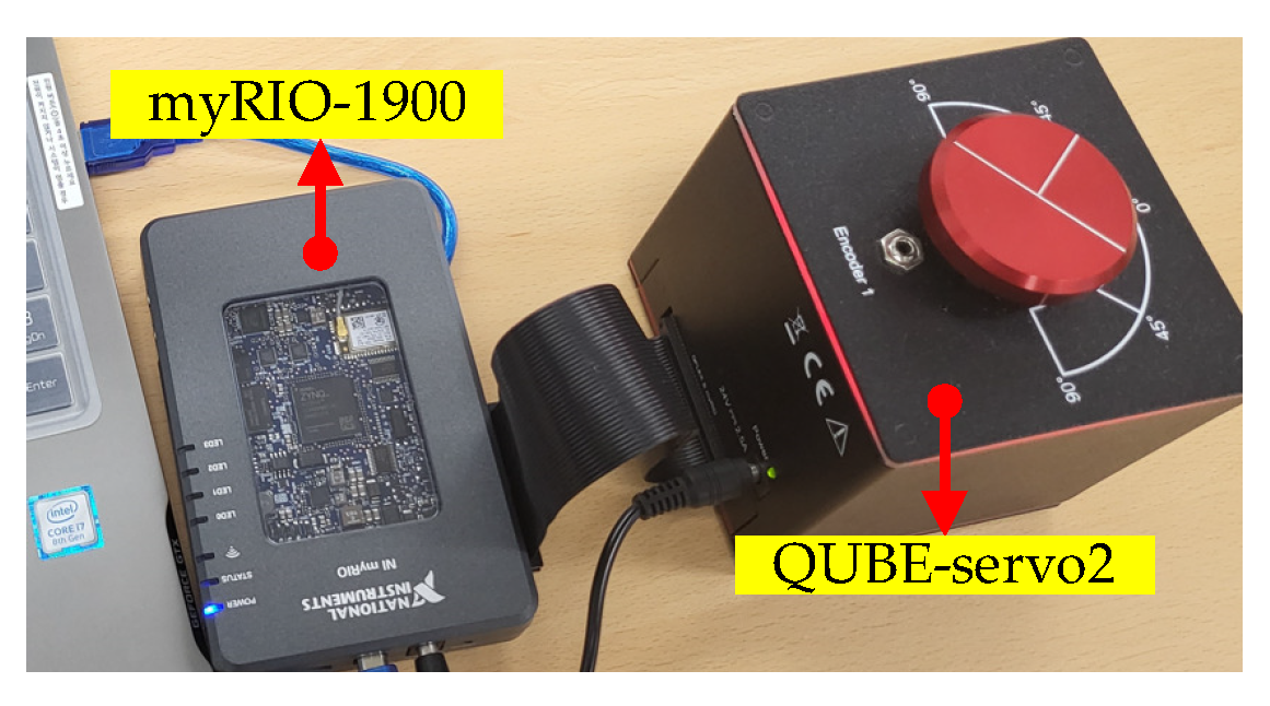
5.1. Set-Up

In this section, the servo system comprising the QUBE-servo2 and myRIO-1900 was used to validate the effectiveness of the proposed technique in reference tracking tasks, which is shown in Figure 2. The datasheet of QUBE-servo2 provided the identification results of the servo machine parameters for J, B, $k_T$, L, R and $k_e$. This section chose their nominal values as $J_0=0.6J$, $B_0=1.2B$, $R_0=0.7R$, $L_0=1.2L$ and $k_{T,0}=k_{e,0}=1.2k_T$, so as to consider the effects of the lumped disturbance $f_{\omega }$ from the model–plant mismatches and load variations. The internal interrupt $0.1$ ms implements the controller (both the inner and outer loops) through a pulse-width modulation of 10 kHz using the LabVIEW software including the MathScript.

This experiment tuned the proposed solution as: $k_{d,e}=3000$ and $f_{{\lambda }_e}=95$ Hz for ${\lambda }_e=600$ for the observer; $f_{sc}=3$ Hz for ${\omega }_{sc}=6\pi$ rad/s for the outer loop control; ${\gamma }_{ac}=5$, ${\rho }_{ac}=2/{\gamma }_{ac}$ and ${\omega }_{ac}=6$ for the adaptive feedback gain; $l_{\omega }=300$ for the DOB; and $k_{d,ac}=0.1$ and ${\lambda }_{ac}=10$ for the acceleration error stabilizer. The following experiments were conducted by comparing the proposed solution to the integral back-stepping controller including the recent active damping compensator (called ADBSC), which was given by: $i_{a,ref}=\frac{1}{k_{T,0}}\left(-k_{d,sc}\omega +J_0{\omega }_{sc}({\omega }_{ref}-\omega )+k_{d,sc}{\int }_0^t({\omega }_{ref}-\omega )d\tau \right)$ for the stator current reference; $v_a=-k_{d,cc}{i}_a+L_0{\omega }_{cc}(i_{a,ref}-i_a)+k_{d,cc}{\omega }_{cc}{\int }_0^t(i_{a,ref}-i_a)d\tau$ for the control input; and the tuned results $k_{d,sc}=0.1$, ${\omega }_{sc}=2\pi f_{sc}$ rad/s with $f_{sc}=3$ Hz and ${\omega }_{cc}=2\pi f_{cc}$ rad/s with $f_{cc}=100$ Hz for the current-loop cut-off frequency for the best performance.

5.2. Tracking Comparison for Stair Speed Reference

This experiment evaluated the stair reference tracking performance of the proposed controller and the ADBSC and the main comparison results for the speed and stator current responses are presented in Figure 3. The left-hand side of Figure 3 shows that the current-loop independence when using the proposed solution not only effectively reduced the steady-state ripples but also lowered the over/undershoot in transient operations. Meanwhile, the right-hand side of this figure indicates that the adaptive feedback gain reduced the required current level in transient periods by automatically adjusting the inner loop gain (as shown in Figure 4). This benefit (the reduction in maximum current level) could be enlarged for high-power servo system applications and could lead to an increase in power efficiency when using the proposed solution. Figure 5 presents the proposed model-independent observer performance, which shows its capability for rapid estimation error removal. The desired adaptive feedback gain response is shown on the left-hand side of Figure 4, where lowering the steady-state gain improved the closed-loop stability margin. The right-hand side of this figure presents the estimated disturbance that aided the performance of the main control action.

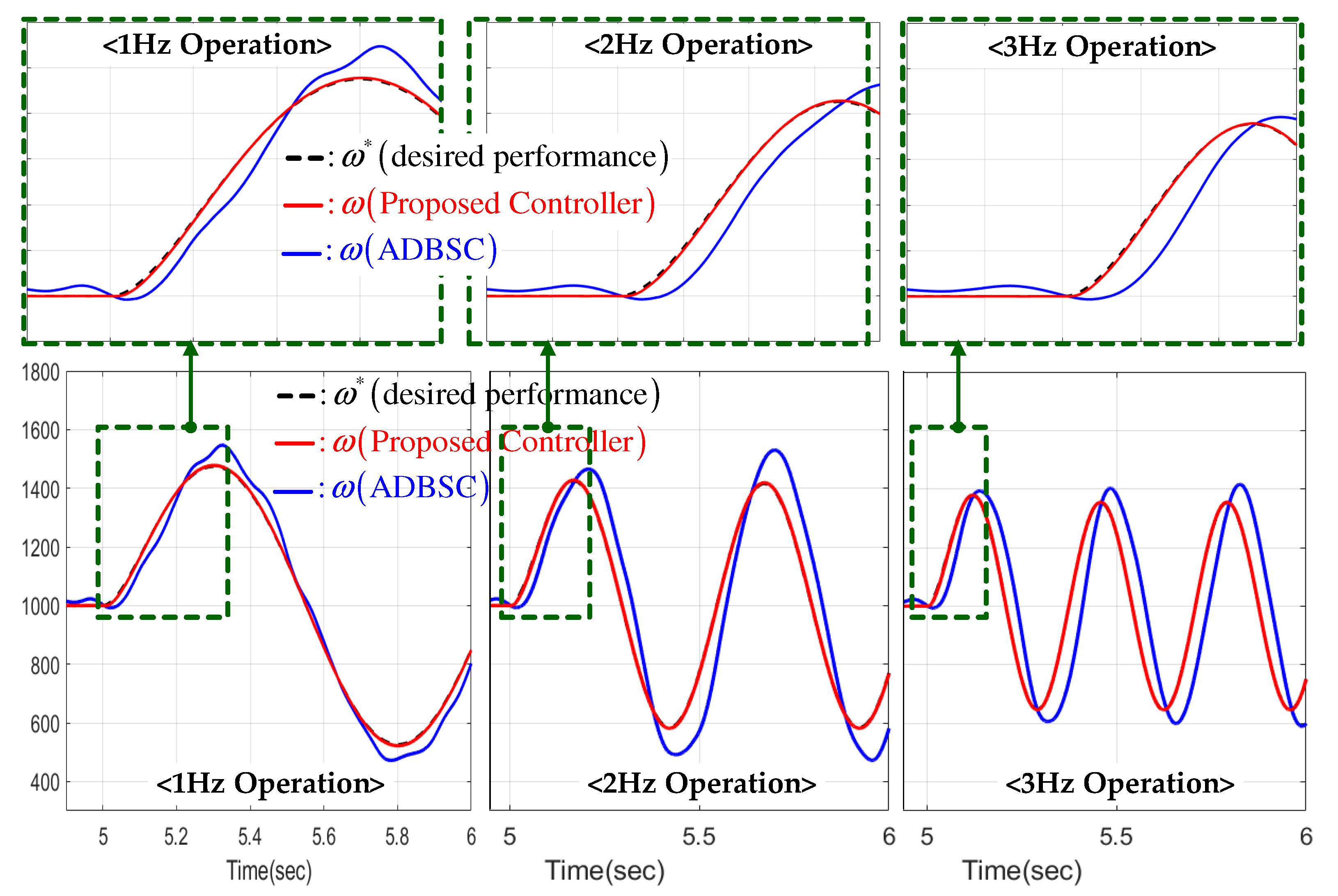
5.3. Frequency Response Comparison

This experiment demonstrated the effectiveness of the proposed solution for the increasing sinusoidal speed references of 1, 2 and 3 Hz. Figure 6 presents the main comparison results. These results show that the proposed controller successfully drove the actual output speed to be almost equal to the desired trajectory ${\omega }^{*}$ from the system in (6) owing to the collaboration of the novel subsystems (the model-independent observer for feedback-free current, active damping and adaptive feedback gain). The ADBSC, however, failed to show this desired performance due to the dependence of the current feedback, which required the additional low-pass filter and caused the phase and magnitude distortions in the current measurements. Figure 7 reveals the decreased stator current using the proposed controller, which resulted in improved power efficiency and was similar to the case of the stair reference tracking comparison in the previous subsection.

6. Conclusions

This study presented a current-feedback independent speed servo system, which included analog to digital converer (ADC) sensitivity for current sensing and a model-independent observer for ensuring order reduction properties in order to eliminate current feedback and strengthen measurement noise. The various closed-loop properties were derived by analyzing the closed-loop dynamics using the Lyapunov stability criterion. The resultant beneficial property (performance recovery) used a low inner loop feedback gain, which was experimentally verified using an experimental servo system comprising QUBE-servo2 and myRIO-1900, and demonstrated the actual robustness improvements, even with errors in the current sensor. However, the proposed controller needed to tune the numerous design factors via an ad-hoc process, which will be solved in a future study incorporating the optimization problems and the constraints that were described by the linear and bilinear matrix inequalities.

References

1. You, S.; Kim, S.K.; Choi, H. Output-Feedback Position Tracking Servo System with Feedback Gain Learning Mechanism via Order-Reduction Speed-Error-Stabilization Approach. Actuators 2021, 10, 324. [Google Scholar] [CrossRef]
2. Chen, Q.; Chen, H.; Zhu, D.; Li, L. Design and Analysis of an Active Disturbance Rejection Robust Adaptive Control System for Electromechanical Actuator. Actuators 2021, 10, 307. [Google Scholar] [CrossRef]
3. Gil, J.; You, S.; Lee, Y.; Kim, W. Back Electro Motive Force Estimation Method for Cascade Proportional Integral Control in Permanent Magnet Synchronous Motors. Actuators 2021, 10, 319. [Google Scholar] [CrossRef]
4. Zakharov, V.; Minav, T. Influence of Hydraulics on Electric Drive Operational Characteristics in Pump-Controlled Actuators. Actuators 2021, 10, 321. [Google Scholar] [CrossRef]
5. Kim, S.K.; Ahn, C.K. Active-damping Speed Tracking Technique for Permanent Magnet Synchronous Motors with Transient Performance Boosting Mechanism. IEEE Trans. Ind. Inf. 2021, 1, 1–9. [Google Scholar] [CrossRef]
6. Park, J.K.; Lee, J.H.; Kim, S.K.; Ahn, C.K. Output-Feedback Speed-Tracking Control Without Current Feedback for BLDCMs Based on Active-Damping and Invariant Surface Approach. IEEE Trans. Circuits Syst. II Express Briefs 2021, 68, 2528–2532. [Google Scholar] [CrossRef]
7. Krause, P.; Wasynczuk, O.; Sudhoff, S. Analysis of Electric Machinery and Drive Systems; Wiley: Hoboken, NJ, USA, 2013. [Google Scholar]
8. Andeescu, G.D.; Pitic, C.; Blaabjerg, F.; Boldea, I. Combined flux observer with signal injection enhancement for wide speed range sensorless direct torque control of IPMSM drives. IEEE Trans. Energy Convers. 2008, 23, 393–402. [Google Scholar] [CrossRef]
9. Tang, L.; Zhong, L.; Rahman, M.; Hu, Y. A novel direct torque control for interior permanent-magnet synchronous machine drive with low ripple in torque and flux - a speed-senseroless approach. IEEE Trans. Ind. Appl. 2003, 39, 1748–1756. [Google Scholar] [CrossRef]
10. Olalla, C.; Leyva, R.; Queinnec, I.; Maksimovic, D. Robust Gain-Scheduled Control of Switched-Mode DC-DC Converters. IEEE Trans. Power Electron. 2012, 27, 3006–3019. [Google Scholar] [CrossRef]
11. Sun, X.; Li, T.; Zhu, Z.; Lei, G.; Guo, Y.; Zhu, J. Speed Sensorless Model Predictive Current Control Based on Finite Position Set for PMSHM Drives. IEEE Trans. Transp. Electrif. 2021, 7, 2743–2752. [Google Scholar] [CrossRef]
12. Sul, S.K. Control of Electric Machine Drive Systems; Wiley: Hoboken, NJ, USA, 2011; Volume 88. [Google Scholar]
13. Kwon, B.; Kim, S.I. Recursive Optimal Finite Impulse Response Filter and Its Application to Adaptive Estimation. Appl. Sci. 2022, 12, 2757. [Google Scholar] [CrossRef]
14. Zhang, Y.; Zhang, S.; Gao, Y.; Li, S.; Jia, Y.; Li, M. Adaptive Square-Root Unscented Kalman Filter Phase Unwrapping with Modified Phase Gradient Estimation. Remote Sens. 2022, 14, 1229. [Google Scholar] [CrossRef]
15. Lin, C.Y.; Yao, W.S. Analysis and Design Multiple Layer Adaptive Kalman Filter Applied to Electro-Optical Infrared Payload Vision System. Electronics 2022, 11, 677. [Google Scholar] [CrossRef]
16. Kim, S.K.; Lee, J.S.; Lee, K.B. Self-Tuning Adaptive Speed Controller for Permanent Magnet Synchronous Motor. IEEE Trans. Power Electron. 2017, 32, 1493–1506. [Google Scholar] [CrossRef]
17. Kim, S.K. Robust adaptive speed regulator with self-tuning law for surfaced-mounted permanent magnet synchronous motor. Control Eng. Pract. 2017, 61, 55–71. [Google Scholar] [CrossRef]
18. El-Sousy, F.F.M.; Abuhasel, K.A. Nonlinear Robust Optimal Control via Adaptive Dynamic Programming of Permanent-Magnet Linear Synchronous Motor Drive for Uncertain Two-Axis Motion Control System. IEEE Trans. Ind. Appl. 2020, 56, 1940–1952. [Google Scholar] [CrossRef]
19. Kim, S.K.; Kim, Y.; Ahn, C.K. Energy-Shaping Speed Controller With Time-Varying Damping Injection for Permanent-Magnet Synchronous Motors. IEEE Trans. Circuits Syst. II Express Briefs 2021, 68, 381–385. [Google Scholar] [CrossRef]
20. Kim, S.K.; Ahn, C.K. Position Regulator With Variable Cut-Off Frequency Mechanism for Hybrid-Type Stepper Motors. IEEE Trans. Circuits Syst. I Regul. Pap. 2020, 67, 3533–3540. [Google Scholar] [CrossRef]
21. Errouissi, R.; Ouhrouche, M.; Chen, W.H.; Trzynadlowski, A.M. Robust Cascaded Nonlinear Predictive Control of a Permanent Magnet Synchronous Motor With Antiwindup Compensator. IEEE Trans. Ind. Electron. 2012, 59, 3078–3088. [Google Scholar] [CrossRef]
22. Son, Y.I.; Kim, I.H.; Choi, D.S.; Shim, H. Robust Cascade Control of Electric Motor Drives Using Dual Reduced-Order PI Observer. IEEE Trans. Ind. Electron. 2015, 62, 3672–3682. [Google Scholar] [CrossRef]
23. Corradini, M.L.; Ippoliti, G.; Longhi, S.; Orlando, G. A Quasi-Sliding Mode Approach for Robust Control and Speed Estimation of PM Synchronous Motors. IEEE Trans. Ind. Electron. 2012, 59, 1096–1104. [Google Scholar] [CrossRef]
24. Ahmed, A.A.; Koh, B.K.; Lee, Y.I. A Comparison of Finite Control Set and Continuous Control Set Model Predictive Control Schemes for Speed Control of Induction Motors. IEEE Trans. Ind. Inf. 2018, 14, 1334–1346. [Google Scholar] [CrossRef]
25. Tao, T.; Zhao, W.; Du, Y.; Cheng, Y.; Zhu, J. Simplified Fault-Tolerant Model Predictive Control for a Five-Phase Permanent-Magnet Motor With Reduced Computation Burden. IEEE Trans. Power Electron. 2020, 35, 3850–3858. [Google Scholar] [CrossRef]
26. Park, R.H. Two-Reaction Theory of Synchronous Machines Generalized Method of Analysis. AIEE Trans. 1929, 48, 716–727. [Google Scholar] [CrossRef]
27. Khalil, H.K. Nonlinear Systems; Prentice Hall: Hoboken, NJ, USA, 2002. [Google Scholar]
Figure 1. Configuration of the proposed solution.
Actuators 11 00126 g001
Figure 2. Servo system implementation for the experimental study.
Actuators 11 00126 g002
Figure 3. Comparison of speed and stator current responses in stair speed reference tracking mode.
Actuators 11 00126 g003
Figure 4. Comparison of adaptive feedback gain and DOB responses in stair speed reference tracking mode.
Actuators 11 00126 g004
Figure 5. Comparison of observer responses in stair speed reference tracking mode.
Actuators 11 00126 g005
Figure 6. Comparison of speed responses for increasing sinusoidal speed references of 1, 2 and 3 Hz.
Actuators 11 00126 g006
Figure 7. Comparison of stator current responses for increasing sinusoidal speed references of 1, 2 and 3 Hz.
Actuators 11 00126 g007
Publisher’s Note: MDPI stays neutral with regard to jurisdictional claims in published maps and institutional affiliations.