Communication

Nonlinear Gaussian Filter with Multi-Step Colored Noise

1
College of Automation Engineering, Nanjing University of Aeronautics and Astronautics, Nanjing 210016, China
2
School of Electronic and Information Engineering, Changshu Institute of Technology, Changshu 215500, China
3
Institute of Changshu, Dalian University of Technology, Changshu 215500, China
*
Author to whom correspondence should be addressed.
Actuators 2022, 11(4), 103; https://doi.org/10.3390/act11040103
Submission received: 6 February 2022 / Revised: 22 March 2022 / Accepted: 23 March 2022 / Published: 29 March 2022
(This article belongs to the Special Issue Resilient Control and Estimation in Networked Systems)

Abstract

:
Color noise is a special kind of noise often occurring in localization systems, and it is more suitable than the general Gaussian white noise to model time dependence due to time delay or high-frequency sampling. This paper derives a nonlinear Gaussian filtering framework for multi-step colored noise systems using noise whitening techniques and Bayes rule. Meanwhile, the cubature rule is used to solve the Gaussian-weighted integral in the proposed Gaussian filtering framework, resulting in an analytic form of posterior state estimate. Compared with the existing nonlinear filtering algorithms, the proposed method has obvious advantages in colored noise systems because it fully takes into account the time dependence of colored noise. Finally, the effectiveness and advantages of the proposed algorithm are verified with a classical target tracking system.

1. Introduction

Nonlinear estimation is a hot problem in engineering and has a wide range of applications in robot control [1,2], fault diagnosis [3], and mobile communications [4]. In the sense of minimum mean square error (MMSE), the optimal state estimate is the mean of its posterior probability density function (PDF). For the linear Gaussian case, the Kalman filter (KF) [5] gives the recursive form of the posterior PDF. However, for the nonlinear systems, the analytic solution of the posterior PDF is difficult to be obtained, in which case one has to find the suboptimal solution. The nonlinear Gaussian filter (GF) [6] derives the approximate state posteriori PDF through a series of Gaussian assumptions, but it involves a series of Gaussian weighted integrals, which are computationally significant. For this reason, a great deal of work has been devoted to search for high-precision numerical methods to approximate the Gaussian weighted integral [7,8,9,10,11]. Unscented Kalman filter (UKF) [8] makes use of unscented transformation (UT) to approximate the Gaussian weighted integral, which is comparable in accuracy to the third-order Taylor expansion. However, the weights of UKF can be negative at high state dimensions, which makes it numerical unstable. Cubature Kalman filter (CKF) [7] uses the three-degree radial rule to compute Gaussian weighted integrals, which has the same accuracy as UKF, and the weights are all positive, making it more stable than UKF. Moreover, there are also Gauss-Hermite quadrature filter (GHQF) [9], High-degree CKF (HCKF) [10] and Sparse-grid quadrature filter (SGQF) [11], etc., all of which are proposed for the idea of improving the accuracy of numerical integration.
However, the above algorithm is only applicable to the system with Gaussian white noise, which is difficult to be satisfied in real-world environments. For example, in complex underwater environments, gravity sensors that commonly used for navigation are susceptible to outliers, which cause their measurement noise to be heavy-tailed. To reflect the heavy-tailed characteristic, the student-t distribution is often used to model the statistical properties of the noise [12]. In channel estimation, no radio links are individually assigned and there is interference between different links, which makes the noise in the channel often a mixture of multiple Gaussian noises, i.e., Gaussian mixture noise [13]. In addition, in GPS navigation systems, the sensors suffer from unavoidable random delays, which makes the noise present at one moment have an impact on the measurements at multiple later moments, i.e., the system suffers from colored noise [14]. In addition, in high-frequency sampling systems and networked systems, color noise can occur. To reduce the impact of color noise on the system, a large amount of literature has been contributed. Refs. [15,16] considered the speech signals with the multi-order colored measurement noise, and respectively proposed the dual perceptually constrained UKF and the modified unscented particle filter (UPF). Refs. [17,18] modelled the measurement noise as the coloured first-order AR process, and proposed the improved UKFs to estimate the multi-path parameter of weak signal from GPS and track the target, respectively. However, the algorithm mentioned above are only applicable to the case of first-order colored noise. In the fields of target tracking, the system noise may be multi-step colored noise [19].
Motivated by the aforementioned analysis, this paper aims to propose a nonlinear filtering algorithm that is applicable to arbitrary order colored noise. The main contributions are summarized as follows: (i) A new system whose noise item is Gaussian white noise is developed by whitening and dimension expansion; (ii) A nonlinear Gaussian filter for the new system is designed by using Gaussian update rule. Finally, a target localization system are used to show the effectiveness and advantages of the proposed methods.
Notations: R r and R r × s denote the r-dimensional and r × s dimensional Euclidean spaces, respectively. E { · } denotes mathematical expectation. diag { · } stands for block diagonal matrix. blk { · } denotes block matrix. O i j R i j is zero matrix. I stands for identity matrix. e i denotes the i-th column of I. Superscript T represents transpose. | · | denotes absolute value. The symmetric terms in a symmetric matrix are denoted by “*”. A A T A ( * ) T , where A is an arbitrary matrix. N ( a ; a ¯ , b ) indicates that random vector a follows Gaussian distribution with mean a ¯ and covariance b.

2. Problem Statement

Consider a nonlinear system described by the following state-space model:
x k + 1 = f ( x k ) + ω k z k + 1 = h ( x k + 1 ) + υ k k = 0 , 1 , 2 ,
where x k + 1 R n x and z R n z are the state vector and measurement, respectively. f ( · ) and h ( · ) represent the nonlinear vector function. ω k and υ k are multi-step colored noise with multi-step autoregressive models, witch can be formulated as
ω k = i = 0 n a k i ω k i + ξ k υ k = i = 0 m b k i υ k i + η k k = 0 , 1 , 2 ,
where n = m i n { k , s } and m = m i n { k , t } are the known correlated step, a k 0 = O n x × n x , b k 0 = O n z × n z , k = 1 , 2 , ξ k and η k are uncorrelated white Gaussian noise with covariance Q k and R k , respectively. a k i , i = 1 , 2 , , n and b k j , j = 1 , 2 , , m are known correlation parameters. Gaussian filtering is done by approximating the system with Gaussian distribution to obtain posteriori estimates
x k | k = E [ x k | z 1 : k ] , P k , k | k x x = E [ ( x k x k | k ) ( * ) T | z 1 : k ]
based on the measurement information z 1 : k = { z 1 , z 2 , , z k } . However, ω k and υ k in system (1) are not Gaussian white noise, and the classical Gaussian filtering is no longer applicable here. Our aim is to design a new Gaussian filter to obtain a posteriori estimates of system (1).
Remark 1: 
It should be emphasized that a k 0 and b k 0 are only added to facilitate the modeling of the case where the colored noise is of order 0. Although it appears in the model, the computational procedure for the terms associated with these two values will not be given later since they are equal to zero matrices and remain zero matrices when multiplied by any matrix.
Remark 2: 
When the sampling frequency of the system is sufficiently high, the noise at a given moment can have an effect on several adjacent sampling periods, and the noise is correlated in the time direction, which is referred to as multi-step colored noise [18]. In addition, feedback control is also one of the causes of colored noise, for example, in the GPS multi-path delay nonlinear estimation, the formation process of the colored noise is shown in Fig. 1 of Ref. [18]. ζ ( t ) = n c ( t ) is the result of input noise n ( t ) spread over the local code, ψ ( t ) = B I p f is the low-pass filter bandwidth equivalent to the integral totalizer.

3. Main Results

3.1. Colored Noises Whitening

In order to process the colored noise in system (1), it is first necessary to whiten it:
y k + 1 = z k + 1 b k + 1 0 z k + 1 b k + 1 1 z k b k + 1 m z k + 1 m = h ( x k + 1 ) b k + 1 0 h ( x k + 1 ) b k + 1 1 h ( x k ) b k + 1 m h ( x k + 1 m ) + η k .
We can see that the noise term of y k + 1 is Gaussian white noise. Moreover, notice that the new measurement y k + 1 becomes a function of x k + 1 m , x k + 2 m ,…, x k + 1 , and the process noise is colored noise. In this case an expansion of the state is required:
X k + 1 = x k + 1 ρ k ω k θ k 1 = f ( x k ) + i = 0 n a k i ω k i ρ k i = 0 n a k i ω k i θ k 1 + ξ k O m n x × 1 ξ k O m n x × 1
where
ρ k = x k x k + 1 m , θ k 1 = ω k 1 ω k n .
The noise term of X k + 1 becomes Gaussian white noise after dimension expansion, and it is clear that y k + 1 is a function of X k + 1 . Let us define
H ( X k + 1 ) h ( x k + 1 ) b k + 1 0 h ( x k + 1 ) b k + 1 1 h ( x k ) b k + 1 m h ( x k + 1 m ) ,
then
y k + 1 = H ( X k + 1 ) + η k .
Equations (5) and (8) constitute the system with noise whitening processing, and notice that { y 1 , y 2 , , y k } can be transformed back into { z 1 , z 2 , , z k } by the linear transformation in Equation (4), which means that the information contained in y 1 : k and z 1 : k is equivalent, so Equation (3) is equivalent to
x k | k = E [ x k | y 1 : k ] , P k , k | k x x = E [ ( x k x k | k ) ( * ) T | y 1 : k ] .

3.2. Design Gaussian Filter with Multi-Step Colored Noise

In this section, in the case of multi-step colored noise, a posteriori estimates of the k + 1 moments are derived based on the posteriori estimates of the k moments. Firstly, for arbitrary random variable α and β , we define
α i | j = E [ α i | y 1 : j ] α ˜ i | j = α i α i | j P i , j | r α β = E [ α ˜ i | r β ˜ j | r T | y 1 : r ] .
The following Lemma will be used later.
Lemma 1 [20]. 
When the joint PDF of α k and β k conditioned on β l : k 1 is Gaussian, that is, p ( α k , β k | β 1 : k ) is Gaussian, then p ( α k | β 1 : k ) can be computed as Gaussian with mean α k | k and corresponding covariance matrix P k , k | k α α as the unified form:
α k | k = α k | k 1 + K k α ( β k β k | k 1 ) ,
P k , k | k α α = P k , k | k 1 α α K k α P k , k | k 1 β β ( K k α ) T ,
K k α = P k , k | k 1 α β ( P k , k | k 1 β β ) 1 ,
where α k | k 1 = E [ α k | β 1 : k 1 ] , P k , k | k 1 α α = E [ ( α k α k | k 1 ) ( * ) T ] , β k | k 1 = E [ β k | β 1 : k 1 ] , P k , k | k 1 β β = E [ ( β k β k | k 1 ) ( * ) T ] . P k , k | k 1 α β = E [ ( α k α k | k 1 ) ( β k β k | k 1 ) T ] .
Assumption 1: 
Based on the measurement from moments 1 to k, the one-step predictive PDF for X k + 1 and y k + 1 are Gaussian, that is
p ( X k + 1 | y 1 : k ) = N ( X k + 1 ; X k + 1 | k , P k + 1 | k X X ) ,
p ( y k + 1 | y 1 : k ) = N ( y k + 1 ; y k + 1 | k , P k + 1 | k y y ) ,
where X k + 1 | k = E [ X k + 1 | y 1 : k ] , P k + 1 | k X X = E [ ( X k + 1 X k + 1 | k ) ( * ) T ] , y k + 1 | k = E [ y k + 1 | y 1 : k ] , P k + 1 | k y y = E [ ( y k + 1 y k + 1 | k ) ( * ) T ] .

3.2.1. One-Step Prediction

According to the definition in Equation (5), the one-step predictive estimate X k + 1 | k can be given by
X k + 1 | k = E [ X k + 1 | y 1 : k ] = E [ x k + 1 | y 1 : k ] E [ ρ k | y 1 : k ] E [ ω k | y 1 : k ] E [ θ k 1 | y 1 : k ] = x k + 1 | k ρ k | k ω k | k θ k 1 | k
where
x k + 1 | k = E [ x k + 1 | y 1 : k ] = E [ f ( x k ) + ω k | y 1 : k ] = f ( x k ) N ( X k ; X k | k , P k , k | k X X ) d X k + ω k | k .
Since ξ k is uncorrelated with y 1 : k , we have
ω k | k = E [ ω k | y 1 : k ] = E [ a k 0 ω k + a k 1 ω k 1 + + a k n ω k n + ξ k | y 1 : k ] = i = 0 n a k i ω k i | k .
Notice that the posteriori estimate of X k at the previous moment is
X k | k = E [ X k | y 1 : k ] = E [ x k | y 1 : k ] E [ ρ k 1 | y 1 : k ] E [ ω k 1 | y 1 : k ] E [ θ k 2 | y 1 : k ] = E [ ρ k | y 1 : k ] E [ x k m | y 1 : k ] E [ θ k 1 | y 1 : k ] E [ ω k 1 n | y 1 : k ] .
According to Equation (6), we have
E [ θ k 1 | y 1 : k ] = ω k 1 | k ω k 2 | k ω k n | k .
In this case, ρ k | k , θ k 1 | k and ω k i , i = 1 , 2 , , n can be obtained from the posteriori estimate at the previous moment, i.e, X k | k .
Moreover, according to the definition in Equation (5), the one-step predictive error covariance P k + 1 | k X X has the following expressions:
P k + 1 , k + 1 | k X X = E [ ( x ˜ k + 1 | k ρ ˜ k | k ω ˜ k | k θ ˜ k 1 | k ) ( * ) T | y 1 : k ] = P k + 1 , k + 1 | k x x P k + 1 , k | k x ρ P k + 1 , k | k x ω P k + 1 , k 1 | k x θ * P k , k | k ρ ρ P k , k | k ρ ω P k , k 1 | k ρ θ * * P k , k | k ω ω P k , k 1 | k ω θ * * * P k 1 , k 1 | k θ θ .
Next, the terms in Equation (21) will be calculated. The error of state one-step prediction can be represented as
x ˜ k + 1 | k = x k + 1 x k + 1 | k = f ( x k ) E [ f ( x k ) | y 1 : k ] + ω ˜ k | k ,
utilizing the Equation (22), we can obtain
P k + 1 , k + 1 | k x x = E [ ( f ( x k ) E [ f ( x k ) | y 1 : k ] + ω ˜ k | k ) ( * ) T | y 1 : k ] = ( f ( x k ) E [ f ( x k ) | y 1 : k ] ) ( ) T N ( X k ; X k | k , P k | k X X ) ) d X k + i = 0 n ( f ( x k ) E [ f ( x k ) | y 1 : k ] ) ω ˜ k i | k T ( a k i ) T N ( X k ; X k | k , P k | k X X ) d X k + ( i = 0 n ( f ( x k ) E [ f ( x k ) | y 1 : k ] ) ω ˜ k i | k T ( a k i ) T N ( X k ; X k | k , P k , k | k X X ) d X k ) T + P k , k | k ω ω
P k + 1 , k | k x ρ = E [ x ˜ k + 1 | k ρ ˜ k | k T | y 1 : k ] = E [ ( f ( x k ) E [ f ( x k ) | y 1 : k ] + ω ˜ k | k ) ρ ˜ k | k T | y 1 : k ] = ( f ( x k ) E [ f ( x k ) | y 1 : k ] ) ρ ˜ k | k T N ( X k ; X k | k , P k , k | k X X ) d X k + P k , k | k ω ρ
P k + 1 , k | k x ω = E [ x ˜ k + 1 | k ω ˜ k | k T | y 1 : k ] = E [ ( f ( x k ) E [ f ( x k ) | y 1 : k ] + ω ˜ k | k ) ω ˜ k | k T | y 1 : k ] = i = 0 n ( f ( x k ) E [ f ( x k ) | y 1 : k ] ) ω ˜ k i | k T ( a k i ) T N ( X k ; X k | k , P k | k X X ) d X k + P k , k | k ω ω
P k + 1 , k 1 | k x θ = E [ x ˜ k + 1 | k θ ˜ k 1 | k T | y 1 : k ] = E [ ( f ( x k ) E [ f ( x k ) | y 1 : k ] + ω ˜ k | k ) θ ˜ k 1 | k T | y 1 : k ] = ( f ( x k ) E [ f ( x k ) | y 1 : k ] ) θ ˜ k 1 | k T N ( X k ; X k | k , P k , k | k X X ) d X k + P k , k 1 | k ω θ .
According to Equations (2) and (6), the P k , k 1 | k ω θ , P k , k | k ω ω and P k , k | k ρ ω can be given by
P k , k 1 | k ω θ = E [ ω ˜ k | k θ ˜ k 1 | k T | y 1 : k ] = E [ ω ˜ k | k [ ω ˜ k 1 | k ω ˜ k n | k ] T | y 1 : k ] = P k , k 1 | k ω ω P k , k n | k ω ω
P k , k | k ω ω = E [ ω ˜ k | k ω ˜ k | k T | y 1 : k ] = i = 0 n E [ ω ˜ k | k ω ˜ k i | k T | y 1 : k ] ( a k i ) T + Q k = i = 0 n P k , k i | k ω ω ( a k i ) T + Q k
P k , k | k ρ ω = E [ ρ ˜ k ω ˜ k T | y 1 : k ] = i = 0 n E [ ρ ˜ k ω ˜ k i | k T | y 1 : k ] ( a k i ) T = i = 0 n P k , k i | k ρ ω ( a k i ) T ,
where
P k , k j | k ω ω = E [ ω ˜ k | k ω ˜ k j | k T | y 1 : k ] = i = 0 n a k i E [ ω ˜ k i | k ω ˜ k j | k T | y 1 : k ] = i = 0 n a k i P k i , k j | k ω ω , j = 0 , 1 , , n .
In addition, using Equation (19) one can obtain
P k , k | k X X = E [ X ˜ k | k X ˜ k | k T | y 1 : k ] = E [ x ˜ k | k ρ ˜ k 1 | k ω ˜ k 1 | k θ ˜ k 2 | k ( * ) T | y 1 : k ] = E [ ρ ˜ k | k x ˜ k m | k θ ˜ k 1 | k ω ˜ k 1 n | k ( * ) T | y 1 : k ] = P k , k | k ρ ρ P k , k m | k ρ x P k , k 1 | k ρ θ P k , k 1 n | k ρ ω * P k m , k m | k x x P k , k | k x θ P k m , k 1 n | k x ω * * P k 1 , k 1 | k θ θ P k 1 , k 1 n | k θ ω * * * P k 1 n , k 1 n | k ω ω .
Comparing Equations (21) and (31), it can be seen that P k , k | k ρ ρ , P k , k 1 | k ρ θ , and P k 1 , k 1 | k θ θ in Equation (21) can be obtained from Equation (31). Moreover, utilizing Equation (6), one obtains
P k 1 , k 1 | k θ θ = E [ θ ˜ k | k θ ˜ k | k T | y 1 : k ] = P k 1 , k 1 | k ω ω P k 1 , k 2 | k ω ω P k 1 , k n | k ω ω * P k 2 , k 2 | k ω ω P k 2 , k n | k ω ω * * * * * P k n , k n | k ω ω
P k , k 1 | k ρ θ = E [ ρ ˜ k | k ω ˜ k 1 | k ω ˜ k 2 | k ω ˜ k n | k T | y 1 : k ] = P k , k 1 | k ρ ω P k , k 2 | k ρ ω P k , k n | k ρ ω
Therefore, P k i , k j | k ω ω , i , j = 1 , 2 , , n and P k , k i | k ρ ω , i = 1 , 2 , n in Equations (21) and (28) can also be derived from P k , k | k X X .

3.2.2. Measurement Update

Based on Assumption 1 and the previous analysis, we have
p ( X k + 1 | y 1 : k ) = N ( X k + 1 ; X k + 1 | k , P k + 1 , k + 1 | k X X ) .
η k + 1 is uncorrelated with y 1 : k , so, measurement one-step prediction can be obtained by
y k + 1 | k = E [ y k + 1 | y 1 : k ] = E [ H ( X k + 1 ) + η k + 1 | y 1 : k ] = H ( X k + 1 ) N ( X k + 1 ; X k + 1 | k , P k + 1 , k + 1 | k X X ) d X k + 1
The error of measurement one-step prediction is
y ˜ k + 1 | k = y k + 1 y k + 1 | k = H ( X k + 1 ) E [ H ( X k + 1 ) | y 1 : k ] + η k + 1 ,
and thus, we have
P k + 1 , k + 1 | k y y = E [ y ˜ k + 1 | k y ˜ k + 1 | k T | y 1 : k ] = ( H ( X k + 1 ) E [ H ( X k + 1 ) | y 1 : k ] ) ( * ) T × N ( X k + 1 ; X k + 1 | k , P k + 1 , k + 1 | k X X ) d X k + 1 .
P k + 1 , k + 1 | k X y = E [ X ˜ k + 1 | k y ˜ k + 1 | k T | y 1 : k ] = ( X k + 1 X k + 1 | k ) ( H ( X k + 1 ) E [ H ( X k + 1 ) | y 1 : k ] ) T × N ( X k + 1 ; X k + 1 | k , P k + 1 , k + 1 | k X X ) d X k + 1 .
Substituting Equations (34), (35), (37) and (38) into Lemma 1, we have
X k + 1 | k + 1 = X k + 1 | k + K k + 1 X ( y k + 1 y k + 1 | k ) ,
P k + 1 , k + 1 | k + 1 X X = P k + 1 , k + 1 | k X X K k + 1 X P k + 1 , k + 1 | k y y ( K k + 1 X ) T ,
K k + 1 X = P k + 1 , k + 1 | k X y ( P k + 1 , k + 1 | k y y ) 1 .
Obviously, x k + 1 | k + 1 and P k + 1 , k + 1 | k x x can be obtained from X k + 1 | k + 1 and P k + 1 , k + 1 | k X X .

3.3. Implementing the Gaussian Filter Using Third-Degree Spherical-Radial Rule

The previous section derived the posteriori estimate at k + 1 moment based on the posteriori estimate at moment k. However, notice that Equations (23)–(26), (35), (37) and (38) contain integral operations, which have a uniform form:
g ( ϕ ) N ( ϕ ; ϕ ¯ , P ) d ϕ
where ϕ R L , g ( · ) is an arbitrary function. The core of the Gaussian filter is the calculation of the integral in the form of Equation (42). Various methods have been proposed in Refs. [6,7,8,9,10,11] to calculate the above equation. The third-degree spherical-radial rule [7] has been widely used to approximate Equation (42) because of its good integration accuracy, stability, and ease of implementation:
g ( ϕ ) N ( ϕ ; ϕ ¯ , P ) d ϕ i = 1 2 L 1 2 L g ( S μ i + ϕ ¯ )
where
P = S S T , μ i = L e i , i = 1 , 2 , , L L e i n , i = L + 1 , L + 2 , , 2 L .
Using Equation (44) to compute the Gaussian weighted integral in Equations (23)–(26), (35), (37) and (38) yields the Cubature Kalman filter with multi-step colored noise (CKF-MCN) easily, and we summarize the algorithmic procedure of the CKF-MCN in Algorithm 1. In addition, to better understand the operation of CKF-MCN, its main steps are summarized in the form of a flow chart in Figure 1.
Algorithm 1:Cubature Kalman filter with multi-step colored noise.
1:
At k + 1 moment, input X k | k and P k | k X X
2:
Obtain ρ k | k , θ k 1 | k and ω k i | k , i = 1 , 2 , , n from X k | k ;
3:
Calculate ω k | k by Equation (18);
4:
Calculate f ( x k ) N ( X k ; X k | k , P k , k | k X X ) d X k using Equation (42), then get x k + 1 | k ;
5:
Get P k , k | k ρ ρ , P k , k 1 | k ρ θ , P k 1 , k 1 | k θ θ , P k i , k j | k ω ω , i , j = 1 , 2 , , n and P k , k i | k ρ ω , i = 1 , 2 , n from P k | k X X ;
6:
Calculate P k , k 1 | k ω θ and P k , k j | k ω ω , j = 1 , 2 , , n using Equations (27) and (30);
7:
Calculate P k , k | k ρ ω and P k , k | k ω ω using Equations (29) and (28);
8:
Calculate
( f ( x k ) E [ f ( x k ) | y 1 : k ] ) ( ) T × N ( X k ; X k | k , P k | k X X ) ) d X k , ( f ( x k ) E [ f ( x k ) | y 1 : k ] ) ρ ˜ k | k T × N ( X k ; X k | k , P k , k | k X X ) d X k , i = 0 n ( f ( x k ) E [ f ( x k ) | y 1 : k ] ) ω ˜ k i | k T × N ( X k ; X k | k , P k | k X X ) d X k × ( a k i ) T , and
( f ( x k ) E [ f ( x k ) | y 1 : k ] ) θ ˜ k 1 | k T × N ( X k ; X k | k , P k , k | k X X ) d X k by Equation (42);
9:
Obtain P k + 1 , k + 1 | k x x , P k + 1 , k | k x ρ , P k + 1 , k | k x ω and P k + 1 , k 1 | k x θ from Equations (23)–(26), then P k + 1 , k + 1 | k X X can be given by Equation (21);
10:
Calculate H ( X k + 1 ) N ( X k + 1 ; X k + 1 | k , P k + 1 , k + 1 | k X X ) d X k + 1 by Equation (42), and then get y k + 1 | k from Equation (35);
11:
Calculate y k + 1 | k , P k + 1 , k + 1 | k y y and P k + 1 , k + 1 | k X y by Equation (42).
12:
Calculate K k + 1 X from Equation (41);
13:
Calculate X k + 1 | k + 1 and P k + 1 , k + 1 | k + 1 X X ;
14:
x k + 1 | k + 1 and P k + 1 , k + 1 | k + 1 x x can be obtained from X k + 1 | k + 1 and P k + 1 , k + 1 | k + 1 X X
15:
Return to step 1 and implement steps 1–14 for obtaining the estimation of next time;
Remark 3: 
Compared with the extended Kalman filter (EKF), the proposed CKF-MCN has two main advantages: (1). Higher accuracy. The EKF utilizes Taylor expansion to approximate the first-order and second-order moments of the random variable with an accuracy of 1st-order Taylor expansion. However, the CKF-MCN uses cubature rules to approximate the statistical properties of random variables with an accuracy of 3rd-order Taylor expansion; (2). Better application prospects. The EKF is only applicable to white noise systems, while the CKF-MCN is applicable to multi-step colored noise systems.

4. Simulation Examples

In this section, the effectiveness of the proposed CKF-MCN is verified by a target tracking simulation. The motion model [7] of the target is
x k + 1 = 1 sin ( Ω T ) Ω 0 ( 1 cos ( Ω T ) Ω ) 0 0 cos ( Ω T ) 0 sin ( Ω T ) 0 0 1 cos ( Ω T ) Ω 1 sin ( Ω T ) Ω 0 0 sin ( Ω T ) 0 cos ( Ω T ) 0 0 0 0 0 1 x k + ω k
z k + 1 = d k + 1 β k + 1 = ( s x , k + 1 a ) 2 + ( s y , k + 1 b ) 2 tan 1 ( s y , k + 1 s x , k + 1 ) + υ k
where the state of the target x k = [ s x , k v x , k s y , k v y , k η ] T , s x , k and s y , k are respectively the coordinates of x-axis and y-axis direction. v x , k and v y , k denote the velocities of x-axis and y-axis direction, respectively. Ω is the turn rate. a and b are respectively the location of the sensor in the x- and y-coordinates. T is the sample period.
The simulation parameters are selected as follows: initial state is x ^ 0 = [ 1000   m 300   m/s 1000   m 0   m/s 3 π 180 rad/s ] T , P 0 = [ 100   m 2 10   m 2 / s 2 100   m 2 / s 2 10   m 2 / s 2 100   mrad 2 / s 2 ] , T = 0.25   s , R k = [ 100   m 2 10   mrad 2 / m 2 ] , Q k = d i a g ( q 1 G q 1 G q 2 T ) where
G = T 3 3 T 2 2 T 2 2 T q 1 = 0.1   m 2 / s 3 , q 2 = 1.75 × 10 4 / s 3 .
We consider the following scenario:
ω k = i = 0 m i n ( 2 , k ) a k i ω k i + ξ k , a k 1 = 0.25 I , a k 2 = 0.05 I υ k = i = 0 m i n ( 2 , k ) b k i υ k i + η k , b k 1 = 0.6 I , b k 2 = 0.2 I .
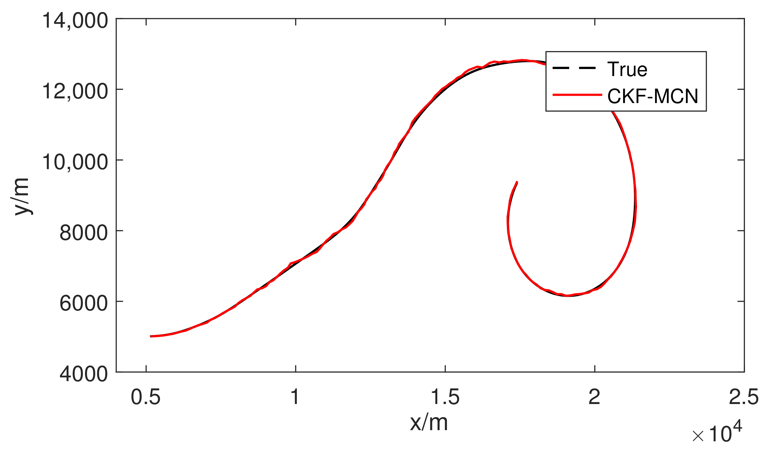
By implementing Algorithm 1, the true and estimated trajectories are plotted in Figure 2. As can be seen from this figure, the CKF-MCN can track the target well. Moreover, position root mean square error (RMSE) is selected as performance indicator to compare the different algorithms, which is given by
RMSE k = 1 m i = 1 m ( s x , k ( i ) s ^ y , k ( i ) ) 2 + ( s y , k ( i ) s ^ y , k ( i ) ) 2
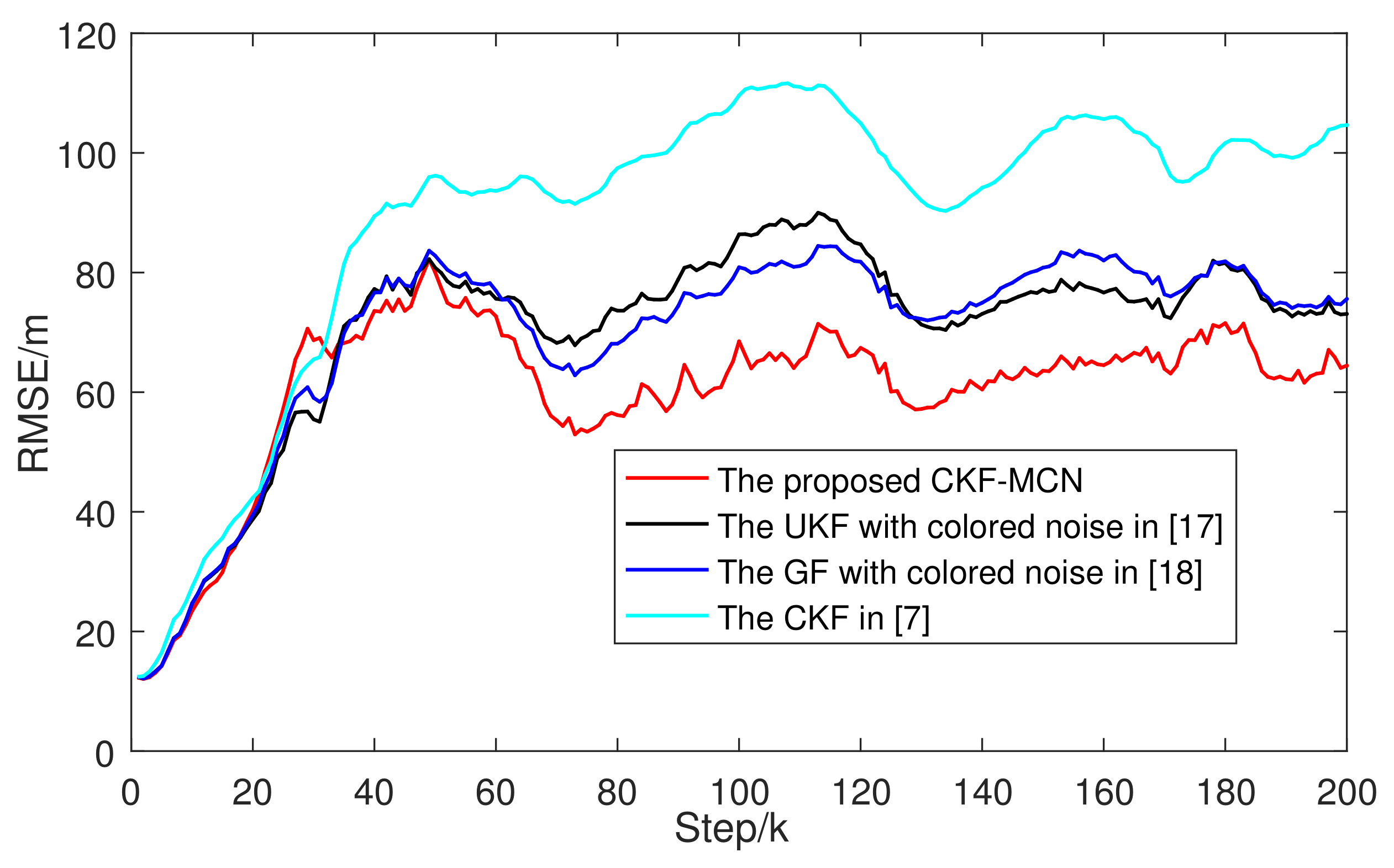
where ( s x , k ( i ) , s y , k ( i ) ) T and ( s ^ x , k ( i ) , s ^ y , k ( i ) ) T are the true and estimated coordinate of target at k instant of the i-th Monte carlo run. To obtain the exact position RMSE, 100 Monte Carlo runs were performed and the simulation results are shown in Figure 3. As can be seen from Figure 3, the CKF-MCN has the highest accuracy in several different methods, which indicates the superior performance of our proposed algorithm in handling multi-step colored noise.

5. Conclusions

In this paper, the problem of state estimation for nonlinear systems with multi-step colored noise is studied. A linear-transform-based technique is proposed to whiten the system with colored noise by which the colored noise system can be transform to an equivalent Gaussian white noise system. A nonlinear Gaussian filtering framework is designed for the whitened system, which is suitable for multi-step colored noise systems. Compared with existing methods that only apply to white noise or first-order colored noise, the proposed method has a wider application scope. Simulation results verify the effectiveness and advantages of the proposed algorithm. Furthermore, it should be emphasized that the proposed menthod expands the dimension of the state, which often leads to the instability of numerical integration. Therefore, in the future work, we aim to propose a new method to solve the state estimation problem under colored noise without dimensionality expansion.

Author Contributions

Conceptualization, software, validation, writing and editing, Y.T.; methodology and review S.S.; funding acquisition, Y.Z. All authors have read and agreed to the published version of the manuscript.

Funding

This work was supported by the Natural Science Foundation of Jiangsu Province under Grant BK20211100.

Conflicts of Interest

The authors declare no conflict of interest.

Abbreviations

x k True state
z k Measurement
w k Color process noise
v k Color measurement noise
X k Whitening state
y k Whitening measurement
ξ k Whitening process noise
η k Whitening measurement noise
y 1 : k The set of measurement from moment 1 to k
X k + 1 | k State one-step prediction of X k + 1
P k + 1 , k + 1 | k X X Covariance one-step prediction of X k + 1
ρ k Augmented state
θ k Augmented process noise
a i | j Mean of a i given y 1 : j
P i , j | k a b Cross-covariance between a i and b j given y 1 : k

References

  1. Aljuboury, A.S.; Hameed, A.H.; Ajel, A.R.; Humaidi, A.J.; Alkhayyat, A.; Mhdawi, A.K.A. Robust Adaptive Control of Knee Exoskeleton-Assistant System Based on Nonlinear Disturbance Observer. Actuators 2022, 11, 78. [Google Scholar] [CrossRef]
  2. Su, Y.; Zheng, C.; Mercorelli, P. Robust approximate fixed-time tracking control for uncertain robot manipulators. Mech. Syst. Sig. Process. 2020, 135, 106379. [Google Scholar] [CrossRef]
  3. Zhou, Y.; Xin, Z.; Fan, Y. Nonlinear filtering application in fault diagnosis. In Proceedings of the 2017 Chinese Automation Congress (CAC), Jinan, China, 20–22 October 2017; pp. 2789–2792. [Google Scholar]
  4. Nunes, F.D.; Leitao, J.M.N. A nonlinear filtering approach to estimation and detection in mobile communications. IEEE J. Sel. Areas Commun. 1998, 16, 1649–1659. [Google Scholar] [CrossRef]
  5. Kalman, R.E. A new approach to linear filtering and prediction problems. ASME J. Basic Eng. 1960, 82, 34–45. [Google Scholar] [CrossRef] [Green Version]
  6. Ito, K.; Xiong, K. Gaussian filters for nonlinear filtering problems. IEEE Trans. Autom. Control 2000, 45, 910–927. [Google Scholar] [CrossRef] [Green Version]
  7. Arasaratnam, I.; Haykin, S. Cubature Kalman filters. IEEE Trans. Autom. Control 2009, 54, 1254–1269. [Google Scholar] [CrossRef] [Green Version]
  8. Julier, S.J.; Uhlmann, J.K. Unscented filtering and nonlinear estimation. IEEE Trans. Autom. Control 2004, 92, 401–422. [Google Scholar] [CrossRef] [Green Version]
  9. Arasaratnam, I.; Haykin, S.; Elliott, R.J. Discrete-time nonlinear filtering algorithms using Gauss-Hermite quadrature. Proc. IEEE 2007, 95, 953–977. [Google Scholar] [CrossRef]
  10. Jia, B.; Xin, M.; Cheng, Y. High-degree cubature Kalman filter. Automatica 2013, 49, 510–518. [Google Scholar] [CrossRef]
  11. Jia, B.; Xin, M. Sparse-grid quadrature nonlinear filtering. Automatica 2012, 48, 327–341. [Google Scholar] [CrossRef]
  12. Wang, Z.; Huang, Y.; Wang, M.; Wu, J.; Zhang, Y. A Computationally Efficient Outlier-Robust Cubature Kalman Filter for Underwater Gravity Matching Navigation. IEEE Trans. Instrum. Meas. 2022, 71, 8500418. [Google Scholar] [CrossRef]
  13. Chen, B.; Petropulu, A.P. Frequency domain blind MIMO system identification based on second- and higher order statistics. IEEE Trans. Signal Process. 2001, 49, 1677–1688. [Google Scholar]
  14. Yuan, G.; Xie, Y.; Song, Y.; Liang, H. Multipath parameters estimation of weak GPS signal based on new colored noise unscented Kalman filter. In Proceedings of the 2010 IEEE International Conference on Information and Automation, Harbin, China, 20–23 June 2010; pp. 1852–1856. [Google Scholar]
  15. Ning, M.; Bouchard, M.; Goubran, R.A. Dual perceptually constrained unscented Kalman filter for enhancing speech degraded by colored noise. In Proceedings of the 7th International Conference on Signal ProcessingSignal Processin, Beijing, China, 31 August–4 September 2004; pp. 2522–2525. [Google Scholar]
  16. Yin, W.; Yi, B.; Shen, X. Speech enhancement based unscented particle filter with non-Gaussian noises. Chin. J. of Radio 2009, 24, 476–481. [Google Scholar]
  17. Xiong, W.; Chen, L.; He, Y.; Zhang, J. Unscented Kalman Filter with Colored Noise. J. Electron. Inf. Technol. 2007, 29, 598–600. [Google Scholar]
  18. Wang, X.; Pan, Q. Nonlinear Gaussian filter with the colored measurement noise. In Proceedings of the 17th International Conference on Information Fusion (FUSION), Salamanca, Spain, 7–10 July 2014; pp. 1–7. [Google Scholar]
  19. Gu, X.; Wang, X.; Zhang, Q.; Zhao, Y. Study on the Filtration and Forecast of Helicopter Tracks under Color Noise Background. J. Detect. Control 2000, 22, 49–53. [Google Scholar]
  20. Zhang, Y.; Huang, Y. Gaussian approximate filter for stochastic dynamic systems with randomly delayed measurements and colored measurement noises. Sci. Chin. (Inf. Sci.) 2016, 59, 161–178. [Google Scholar] [CrossRef] [Green Version]
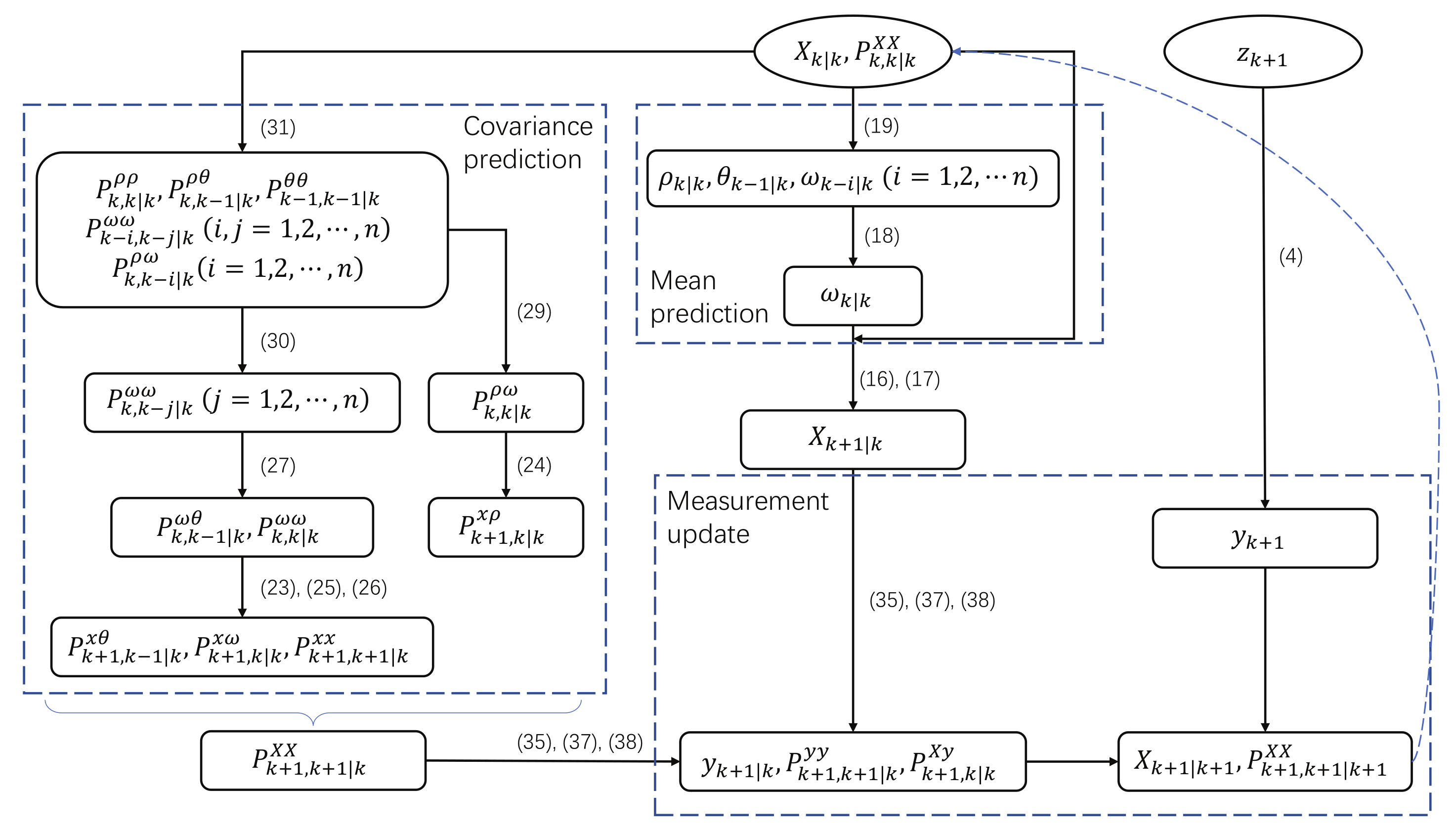
Figure 1. The flowchart of the CKF-MCN.
Actuators 11 00103 g001
Figure 2. True and estimated trajectories by using CKF-MCN.
Actuators 11 00103 g002
Figure 3. Comparisons of the position RMSE obtained by the proposed CKF-MCN, the UKF with colored noise in Ref. [17], the GF with colored noise in Ref. [18] and the CKF in Ref. [7].
Actuators 11 00103 g003
Publisher’s Note: MDPI stays neutral with regard to jurisdictional claims in published maps and institutional affiliations.