Article

Deep Reinforcement Learning for Stability Enhancement of a Variable Wind Speed DFIG System †

Department of Electronics, Carleton University, Ottawa, ON K1S 5B6, Canada
*
Author to whom correspondence should be addressed.
This paper is an extended version of our paper published in: Kosuru, R.; Chen, P.; Liu, S. A Reinforcement Learning based Power System Stabilizer for a Grid Connected Wind Energy Conversion System. In Proceedings of the 2020 IEEE Electric Power and Energy Conference (EPEC); IEEE: Edmonton, AB, Canada, 9 November 2020; pp. 1–5.
Actuators 2022, 11(7), 203; https://doi.org/10.3390/act11070203
Submission received: 1 June 2022 / Revised: 14 July 2022 / Accepted: 15 July 2022 / Published: 20 July 2022
(This article belongs to the Special Issue Resilient Control and Estimation in Networked Systems)

Abstract

:
Low-frequency oscillations are a primary issue for integrating a renewable source into the grid. The objective of this study was to find sensitive parameters that cause low-frequency oscillations and design a Twin Delayed Deep Deterministic Policy Gradient (TD3) agent controller to damp the oscillations without requiring an accurate system model. In this work, a Q-learning (QL)-based model-free wind speed DFIG was designed on the rotor-side converter (RSC), and a QL-based model-free DC-link voltage regulator was designed on the grid-side converter (GSC) to enhance the stability of the system. In the next step, the TD3 agent was trained to learn the system dynamics by replacing the inner current controllers of the RSC, which replaced the QL-based model. In the first stage, the conventional PSS and Proportional–Integral (PI) controllers were introduced to both the RSC and GSC. Then, the system was trained to become model-free by replacing the PSS and the PI controller with a QL algorithm under very small wind speed variations. In the second stage, the QL algorithm was replaced with the TD3 agent by introducing large variations in wind speed. The results reveal that the TD3 agent can sustain the stability of the DFIG system under large variations in wind speed without assuming a detailed control structure beforehand, while QL-based controllers can stabilize the doubly fed induction generator (DFIG)-equipped wind energy conversion system (WECS) under small variations in wind speed.

1. Introduction

Based on the type of generator and the grid interface, wind energy systems can be categorized into four types [1]:
(a)
Squirrel-cage induction generator (SCIG) or fixed speed system.
(b)
Wound-rotor induction generator (WRIG) with variable rotor resistance.
(c)
Doubly fed induction generator.
(d)
Full-power converter generator.
SCIGs are mainly used for smaller wind turbines, as they are simple and economical compared to other generators. In a squirrel-cage induction generator, the rotor bars are permanently short-circuited; therefore, the rotor voltage is zero. The stator is connected to a soft starter and is connected to the grid through a transformer. A capacitor bank is employed to compensate for the reactive power, and a soft starter is employed to mitigate high starting currents and to produce a smooth grid connection [2]. In a WRIG, the stator is directly connected to the grid, and the wound rotor winding is connected to a variable resistor via slip rings. In a WRIG, it is possible for the rotor to have configurations such as slip power recovery, the use of cyclo-converters, and rotor resistance chopper control [3]. In both WRIGs and SCIGs, by controlling the rotor resistance, the slip of the machine can be changed to 2–10% [1], through which the generator output can be controlled. The third type of generator used is the DFIG. The constructional features of DFIGs are like those of WRIGs, except that in a DFIG, the rotor winding of the WRIG is connected to the grid through an AC-DC-AC converter. In a fully converted synchronous generator or fully converted squirrel-cage induction generator (SCIG), the total power is interchanged between the wind system and the grid through a power electronic converter system, whereas in some systems, it can be transmitted to the grid directly [1]. Figure 1a,b show the configuration of a wind system with a synchronous generator and with a permanent-magnet synchronous generator (PMSG) [1]. It can be recognized that in Figure 1a, the synchronous generator is excited by using the power electronic converter externally, while in Figure 1b, it is excited by a permanent magnet, as the generator is a permanent-magnet synchronous generator. For large wind farms, both DFIGs and PMSGs are preferred due to increased power control.
There are many advantages and superior characteristics of using a PMSG machine over a DFIG. A PMSG machine has better performance, higher reliability, and wider speed control [4]. Due to the PMSG’s better performance, most of the current research work focus has shifted to topologies utilizing synchronous generators with permanent-magnet excitation. However, DFIGs are still dominant in modern wind power generation systems, as DFIGs can operate under variable speeds, regulate active and reactive power independently, and have a low converter cost [5]. The reason for the lower converter cost in DFIG wind turbines is that the power electronic devices are fed with power generated only by the rotor (25–30% of rated power), and due to this, the lower converter rating compromise offers significant cost savings over a PMSG [6].
The doubly fed induction generator (DFIG) model is considered one of the best solutions for wind energy conversion systems (WECSs). The two main reasons for using a DFIG in a WECS are its asynchronous characteristics and the flexibility of utilizing power electronic converters, which results in cost savings due to a lower converter rating. In DFIG-based grid-connected wind systems, the stator is directly connected to the grid, whereas the rotor is connected to the grid by using a back-to-back power electronic converter. Figure 2 depicts the schematic model of a grid-connected DFIG-based WECS [7].
Every power network (grid) experiences a lot of disturbances, as there may be a great number of variations, such as voltage, frequency, active power, and reactive power, at the load end or at power generating stations (renewable or non-renewable). For any system to operate without disturbances, power system stability and voltage regulation are critical control issues that need to be considered [8]. The importance of power system stability can be illustrated clearly by investigating [9], which presents a clear description of power system instability as the primary grounds for any major blackout. The main objective of any power system stabilizer is to provide stable power to the grid and to improve the damping of oscillations. Especially when connecting any renewable energy conversion system to the grid, supplying stable power is always challenging due to fluctuating frequencies and voltages.

2. Literature Review

In a DFIG-equipped WECS, decoupled controllers are used to control the active and reactive power on both the rotor and grid sides, the rotor speed, and DC voltage and to track the maximum power. Low-frequency oscillations were observed for a WECS with weak grid interconnections; this oscillation mode caused torsional interconnections with a remote synchronous generator and led to the shutdown of the power plant [10]. To overcome the problem of low-frequency oscillations, a power system stabilizer can be applied at the output or the input of the controller. As per [11], a PSS can be employed for any DFIG variable that is influenced by network oscillations, such as rotor speed, stator electrical power, and voltage or network frequency. In [11,12,13,14,15,16,17,18], the importance of employing a PSS and improving the damping of oscillations in a grid network fed by a DFIG-WES using slip signal and rotor speed deviations are discussed. Various oscillations that are damped using a PSS are: electromechanical oscillations [19], inter-area power system oscillations [20,21], network damping capability [22], and oscillations caused by DFIG when integrated into a network that is already fed by a synchronous generator [17,18]. These papers clearly illustrate the need for a PSS to damp the oscillations and show that a PSS can be used to improve the stability of the grid-integrated wind system.
Most of the conventional PSSs (CPSSs) employed for wind energy systems are classical designs in which the system is linearized around an operating point. However, PSSs developed using Artificial Intelligence (AI) techniques have been used for design and stability studies of non-renewable-sourced power systems. Some of the frequently used techniques for a PSS design are ANN [23,24] and Fuzzy Logic [10,25,26], and support vector regression was used to design an adaptive PSS in [27]. The use of AI to solve stability issues has been categorized into three separate methodologies based on the techniques used: supervised learning, unsupervised learning, and reinforcement learning (RL) [28]. RL is completely different from supervised learning and unsupervised learning. Supervised learning alone is not adequate for learning from interactions, and in interactive problems, it is often impractical for supervised learning to obtain the desired behavior for all situations in which the agent must act [28]. In contrast, in an RL territory, an agent must be able to learn from its own experience. Unsupervised learning is typically focused on finding structures hidden in collections of unlabeled data, whereas the RL paradigm aims to maximize a reward signal instead of trying to find hidden structures [28]. Thus, an RL is a third machine learning paradigm, alongside supervised and unsupervised learning.
The current research used reinforcement learning to control the entire system, as there is a need for interaction between the mechanical system (wind turbine) and electrical system (DFIG and controllers) to supply stable power to the grid for wind speed variations. One of the main reasons for using the RL control method is its capability of adapting itself to evolving generation levels, load levels, and operating uncertainties and responding to arbitrary disturbances [29]. In [29], the RL method was used in online mode and applied to control a thyristor controller series capacitor (TCSC), aiming to damp power system oscillations. RL controllers were designed to stabilize the closed loop system after severe disturbances in [30]. A specific RL algorithm called Q-learning was utilized to control and adjust the gain of a conventional PSS in [31]. The RL algorithm was also used in generation control and voltage and reactive power control [32,33,34]. In [35], a control strategy was developed for a PSS using the Q-learning method to suppress low-frequency oscillations. In [36], a proportional resonance PSS (PR-PSS) was proposed using an actor-critic agent, one of the RL techniques for adaptive adjustment of parameters to suppress ultra-low-frequency oscillations. The RL techniques discussed in [35,36] were used for comparing the PSS results obtained with the Q-learning algorithm discussed in this paper. The TD3 method was implemented in [37,38] for continuous power disturbances to overcome low-frequency oscillations. In [38], the TD3 method was used to perform parameter estimation and the fine-tuning of PID controllers and to overcome the problem of low-frequency oscillations caused by load generation variations. Deep reinforcement learning methods were implemented for load frequency control of a multi-area power system and battery energy management. In [39], a multi-agent deep reinforcement learning method was proposed, which utilized the DDPG method to optimize load frequency control performance. In this study, in addition to the QL method, the TD3 method was explored and implemented to solve the low-frequency oscillations caused by huge variations in wind speed. In this research, the TD3 method and QL method were implemented by replacing the existing PI controller and PSS. This paper is an extension of [40], where a Q-learning algorithm was implemented on the rotor-side converter for a small range of changes in wind speeds. The major contributions of the current work are discussed in Section 3.

3. Contributions

In this work, a CPSS was first designed, and control strategies were applied at a fixed wind speed. The optimal PI gain values for both the rotor-side converter and the grid-side converter were obtained by using eigenvectors for the PSS, and the stability of the system was proved mathematically. In the next step, a Q-learning algorithm was implemented on the designed PSS on the RSC and PI controllers on the GSC for variable wind speeds. The objective of the Q-learning algorithm implemented on the RSC and GSC is to suppress the low-frequency oscillations of the DFIG-based WECS when variable speeds are applied to the system. Since the control objective is to stabilize the system with active power (P) and reactive power (Q) without low-frequency oscillations, this paper uses the active power change as the state of the agent and the control output of the RSC as the action of the agent to train the model. On the grid-side converter, the grid-side active power is controlled, which is a function of DC-link voltage ( V d c ), which acts as the state of the agent, and the reward function generates the input signal to the grid-side current ( i d g * ). Simulation results verify that the designed Q-learning-based model-free controllers can quickly stabilize the DFIG wind system under a small range of wind speeds. The terms action, state, and agent used in this section are explained in detail in Section 3 of this paper. With the Q-learning agent, the system becomes unstable under huge variations in wind speed. One of the solutions is to implement the system with an actor-critic method. In this research, the TD3 agent was trained to learn the system dynamics under huge variations in wind speed and control the active and reactive power. Real-time wind speed variations in the Ottawa region were used as the system input. The PI controller in the inner current control loop of the RSC was replaced with the TD3 agent. From the results discussed in Section 5, it is observed that the TD3 agent can mitigate the frequency changes under huge variations in wind speed and provide stable power to the grid. In both QL and TD3 implementations, the PSS and PI controllers were removed, and the agent was trained to learn the system dynamics and suppress low-frequency oscillations.

4. Wind Turbine System Structure and Model

Figure 2 shows the physical model of the grid-connected DFIG-based wind turbine system. This benchmark power system model was first introduced in [7] to study the effect of shaft systems and low-frequency oscillations by comparing the switching-level (SL) and Fundamental Frequency (FF) models. As illustrated in Figure 2, the system consists of mechanical and electrical models. The mechanical model has 3 different components: (1) wind turbine, (2) gearbox, and (3) pitch controller; all 3 of these components together provide a complete drivetrain model, which provides the required mechanical energy to the generator. The electrical model consists of a DFIG generator, of which the stator is directly connected to the grid, and the rotor is connected through back-to-back IGBT-based pulse-width modulation converters.

4.1. Design of Drivetrain Model

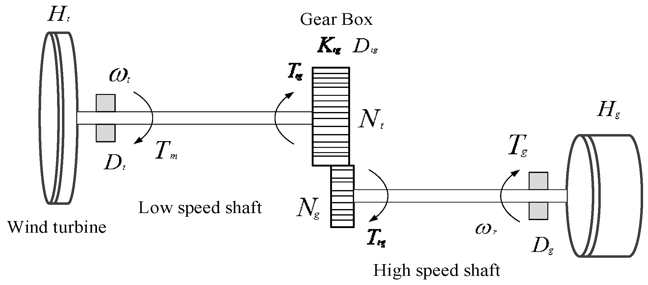
The mathematical representation of the drivetrain is formed by the turbine rotating mass, low-speed shaft, gearbox, high-speed shaft, and generator rotating mass. The model of the drivetrain is developed by neglecting the mechanical twisting and stresses, as these are more related to mechanical design and studies. Moreover, for power system stability studies, it is suggested in [41] to consider the turbine, gearbox, and generator as rigid disks and shafts as mass-less torsional springs. A two-mass model is recommended for power system stability studies; this is because there are more possibilities for the representation of shaft stiffness and inertia constants [42]. Figure 3 shows the physical representation of the two-mass model [7]. The dynamics of the two-mass model can be obtained by applying Newton’s equation of motion for each mass. The equations obtained are [7,43]:
2 H t p ω t = T m D t ω t T s h
2 H g p ω r = T s h D g ω r T e
where p = d / d t , and T s h is the shaft torque, which is given as:
p T t g = K t g ( ω t ω r )
T m = P t ω t
In Figure 3, ω t and ω r are the turbine and generator rotor speeds, respectively. T m and T e are the mechanical torque applied to the turbine and electrical torque, respectively; H t and H g are the turbine inertia constant and generator inertia constant, respectively; D t and D g are the damping coefficients of the turbine and generator, respectively; T t g is the internal torque of the model; D t g is the damping coefficient of the shaft between the two masses; K t g is the spring constant or shaft stiffness. Finally, N t / N g is the gear ratio of the gearbox.

4.2. DFIG Model

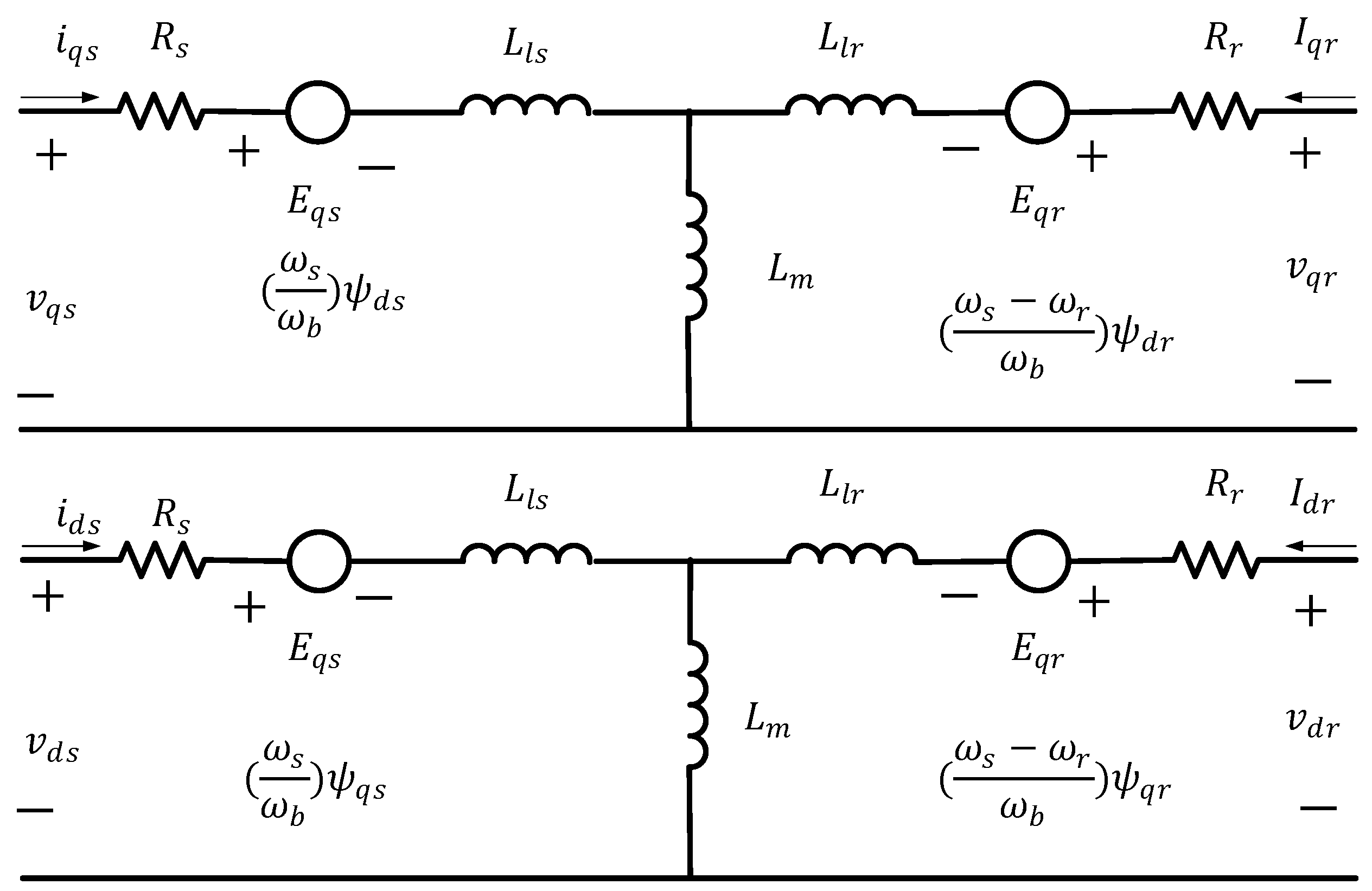
For power system stability studies, the DFIG machine is modeled by neglecting stator transients, as they do not affect the electromechanical oscillations [44], and by neglecting stator transients, it is easier to solve stator and grid equations [45]. Similarly, the rotor electrical transients are also neglected, as rotor winding is controlled by fast-acting converters [46]. In addition, other assumptions that are made for modeling the DFIG are: the skin effect, the saturation effect, and iron losses (hysteresis and eddy currents) are neglected, as these phenomena contribute more to conducting loss performance in transient fault analysis. For designing the DFIG, a synchronous reference frame is used. The reason for representing the DFIG model in a synchronous rotating reference frame is because the q d -axis model is convenient for conducting steady-state analysis and deriving a small-signal model [47]. The equivalent circuit of a DFIG in a synchronously rotating reference frame is given in Figure 4.
In Figure 5, the q - and d -axes are orthogonal to each other, rotating at an angular velocity of ω , whereas a s , b s , and c s represent stator variables displaced by 120 ° . To analyze the induction machine variable associated with the rotor, the reference frame also needs to be transformed to q d -axis reference frame. In Figure 5, a r , b r , and c r represent rotor variables displaced by 120 ° , rotating at an angular velocity of ω r .
The stator model is represented in the q d -axis reference frame.
v d s = R s i d s ω s ω b ψ q s + p ψ d s
v q s = R s i q s + ω s ω b ψ d s + p ψ q s
The rotor model is represented in the q d -axis reference frame.
v d r = R r i d r ( ω s ω r ω b ) ψ q r + p ψ d r
v q r = R r i q r + ( ω s ω r ω b ) ψ d r + p ψ q r
The mathematical model including the saturation effect is provided below [48].
i m d = i d s + i d r
i m q = i q s + i q r
i m = i m d 2 + i m q 2
L m s = ψ m i m   &   L m d = d d i m ( ψ m )
The voltage equations of the DFIG with flux saturation are:
v d s = R s i d s ω s ω b ( L s i q s + L m s i m q ) + L s p i d s + L m d p i m d
v q s = R s i q s + ω s ω b ( L s i d s + L m s i m d ) + L s p i q s + L m d p i m q
v d r = R r i d r ( ω s ω r ω b ) ( L r i q r + L m s i m q ) + L r p i d r + L m d p i m d
v q r = R r i q r + ( ω s ω r ω b ) ( L s i d r + L m s i m d ) + L r p i q r + L m d p i m d
where p = d d t .

4.3. Control Strategies

To develop control strategies for the converters, any one of the axes in two reference frames ( q d ) , rotating with synchronous speed, is aligned with either the flux or the voltages of the stator. The two commonly used control strategies are stator flux-oriented control and stator voltage-oriented control. In stator flux-oriented control, the d -axis is aligned with the stator flux linkage vector [7]. This results in ψ d s = ψ s and ψ q s = 0 . In contrast, in stator voltage-oriented control, the d -axis is aligned with the stator voltage linkage vector, resulting in V d s = V s and V q s = 0 . For rotor-side converter control, stator flux-oriented control is used, and for grid-side converter control, stator voltage-oriented control is adopted [7]. For this work, stator voltage-oriented control is implemented for both the rotor-side converter controller and grid-side converter controller, as discussed in [49]. Compared to flux-oriented control, voltage-oriented control has the advantage of deriving the model and aligning with the stator voltage space vector using the measured phase voltages. Another advantage is that, typically, the grid-side converter is controlled using the stator voltage orientation, so by choosing voltage-oriented control for the rotor-side controller, the model will be simpler to implement. The usage of voltage-oriented control on both the RSC and GSC can be observed in [49]. The objective of these control strategies is to decouple the control of active and reactive power [49].

4.4. Rotor-Side Controllers

The main objective of the rotor-side converter controller is to control both the active and reactive power of the stator. It consists of two control loops: the inner control loop regulates the d - and q -axis rotor currents, whereas the outer loop controls the active P s and reactive Q s power of the generator stator. By neglecting the transients in the stator flux linkages in the stator voltage orientation and under the assumption that resistive drops are negligible, it is observed that active power P s is independent of the q -axis rotor current. Under the same assumptions for the rotor model, the stator reactive power Q s is totally dependent on the q -axis rotor current, and it is independent of the d -axis rotor current. It can be concluded that, in the RSC, the stator active and reactive power can be controlled independently by rotor d -axis and q -axis currents, respectively, which generates stator active and reactive power reference current outputs i d r * and i q r * , respectively.
The generated reference currents are fed as inputs to the inner current loops of the rotor current controller. The final outputs of the rotor-side converter controller are v d r and v q r . The controller is designed based on the rotor voltage models, which can be expanded from Equations ( 17 ) and ( 18 ) and expressed as [49]:
v d r = R r i d r ( ω s ω r ) ( L r i q r + L m i q s ) + p ( L r i d r + L m i d s )
v q r = R r i q r + ( ω s ω r ) ( L r i d r + L m i d s ) + p ( L r i q r + L m i q s )
When designing the rotor-side controller with decoupling elements, if the transients of the machine are neglected, the derivative terms become zero. With this condition, the d -axis rotor voltage will be in terms of i d r ; similarly, the d -axis rotor voltage will be in terms of i q r . With these elements, a transfer function can be developed for the inner current control loops, and from this, the PI gains are obtained. From the mathematical models developed, it is observed that the design is the same for both control loops, so the P I control design is also the same for both inner current control loops. In these control loops, v d r 1 and v q r 1 are the outputs of the rotor current controller loops, and they are fed to the pulse-width modulator of the converter along with the decoupled elements. Finally, these obtained signals from the modulator are fed to the converter circuit, and this is connected to the DC link of the model.
In Figure 6, i d r and i q r are the rotor currents, and they are transformed from rotor three-phase currents i r a b c to i r d q by applying a transforming angle of ( θ s θ r ) , where θ s is the angle obtained from v s a b c at the grid frequency, and θ r is the rotor angle. P s is the stator active power, and Q s is the stator reactive power, and these are obtained from v s a b c and i s a b c . Reactive power reference Q s r e f is given as 0 , whereas stator active power reference P s r e f is generated using the maximum power tracking method. In this work, a simple lookup table is used, which tries to obtain the reference stator power by plotting power and speed. The other reference at v d r control is the generator reference value, which is set by the speed.

4.5. Grid-Side Controllers

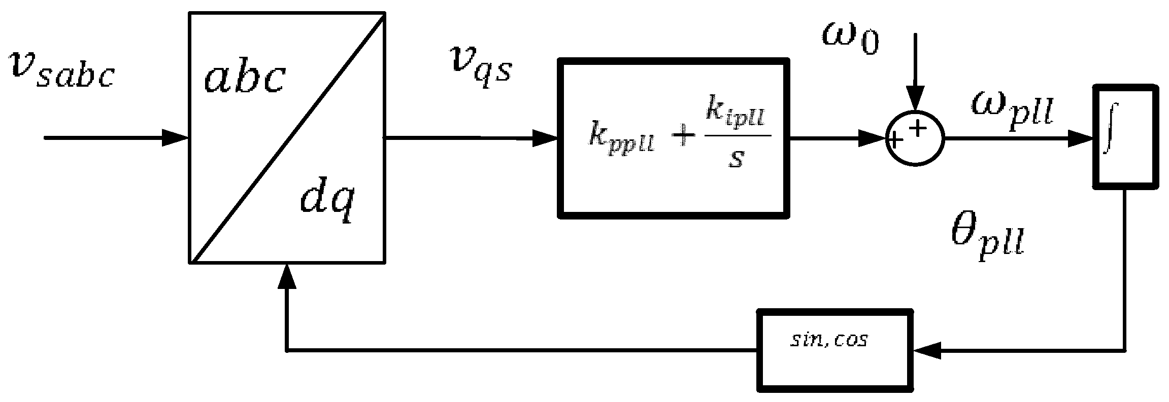
To design the grid-side converter controller, first, the grid model in the a b c reference frame is transformed into two reference frames by using a phase-locked loop (PLL), which provides the required transformation angle and the frequency for synchronizing the model with the grid. The design and operation of the PLL are derived from [50], and it is shown in Figure 7 [50]. The grid model in the a b c reference frame is transformed to the d q reference frame based on the transformation matrix from Equation ( 19 ) [50].
The transformation angle θ is the grid-side converter terminal voltage angle, and it is expressed as θ = ω 0 t + δ , where δ is given as p δ = ω ω 0 , where ω is the grid-side converter terminal frequency. The phase angle measured by the PLL is given as θ p l l , and the measured frequency is given as ω p l l ; this provides the transformation angle and the frequency to the grid-side converter controller design. The obtained angle and frequency information is used for both a b c d q and d q a b c transformation at the grid end.
[ v d v q ] = 2 3 [ cos θ cos ( θ 2 π 3 ) cos ( θ + 2 π 3 ) sin θ sin ( θ 2 π 3 ) sin ( θ + 2 π 3 ) ] [ v a v b v c ]
Initially, for operating the PLL, the q -axis voltage of the stator v q s is obtained by the a b c d q transformation technique. Once the grid-side converter terminal voltage is transformed and the transformation angle is θ p l l , then the obtained equation is v q s = V sin ( θ θ p l l ) = V sin ( δ δ p l l ) , where δ p l l is the measured phase angle and is expressed as δ p l l = θ p l l ω 0 t . The grid-side voltage frequency ω p l l is obtained by adding the error signal processed in the PI controller and ω 0 , and it is given as:
ω p l l = ( k p p l l + k i p l l s ) v q s + ω 0
p δ p l l = ω p l l ω 0
By using this three-phase PLL, the grid equations can be transformed into two reference frames. The d q -transformed equations of the grid model are as follows:
v d s = r i d + L p i d ω p l l L i q + e d
v q s = r i q + L p i q ω p l l L i d + e q
In Equations ( 22 ) and ( 23 ) , v d s and v q s are the stator voltages; r and L are the grid filter resistance and inductance, respectively; and i d and i q are the total currents supplied to the grid in the d q reference frame. Finally, e d and e q are the transformed voltages of the grid terminal. The model for the total current supplied to the grid, i.e., i d and i q , are given as the sum of the stator currents i d q s and grid-side converter currents i d q g . The grid-side converter voltages in the d q reference frame can be expressed as:
v d g = R g i d g + L g p i d g ω p l l L g i q g + v d s
v q g = R g i q g + L g p i q g + ω p l l L g i d g + v q s
Finally, the grid voltages are expressed as:
e d = E cos ( δ p l l )
e q = E sin ( δ p l l )
From the above-derived grid-side model, the grid-side converter controller can be designed. The main objective of the grid-side converter controller is to regulate the DC-link voltage and exchange power between the rotor-side converter and the grid. The other objective of this controller is to control the reactive power that is delivered to the grid at the grid-side converter. Like the rotor-side converter controller, the grid-side converter controller also consists of two cascaded control loops. The DC-link voltage and the reactive power are controlled by the outer control loop, whereas the inner current control loop regulates the current components in the grid-side converter. From the above-discussed grid model, the active power and the reactive power at the grid can be expressed as:
P g c = 3 2 ( v d s i d g + v q s i q g )
Q g = 3 2 ( v q s i d g v d s i q g )
For grid-side active power in these equations, by applying the synchronously rotating reference frame and aligning the d -axis on the grid voltage vector, the obtained results are v d s = v s and v q s = 0 . Applying this to Equations ( 24 ) and ( 25 ) yields:
v d g = R g i d g + L g p i d g ω p l l L g i q g + v d s
v q g = R g i q g + L g p i q g + ω p l l L g i d g
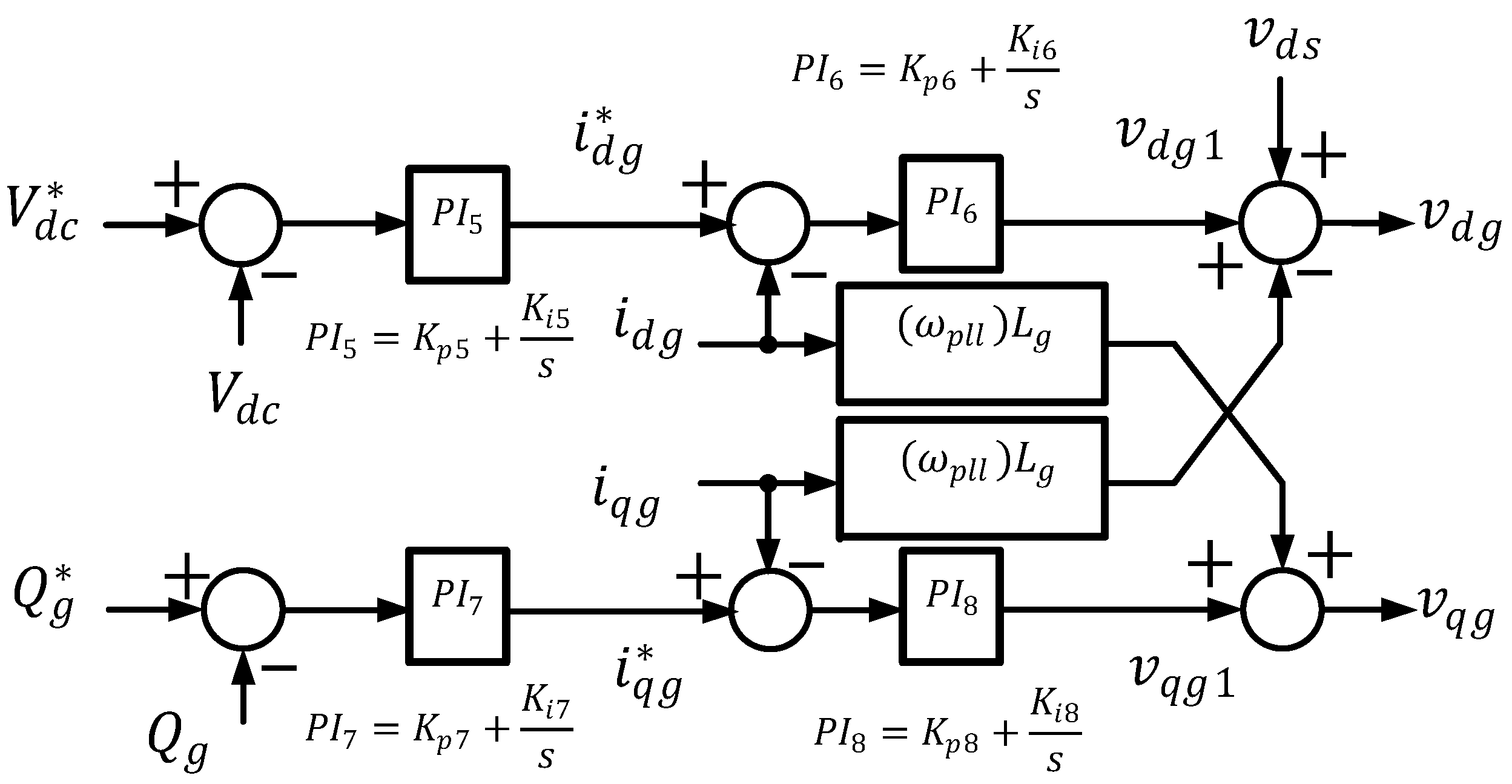
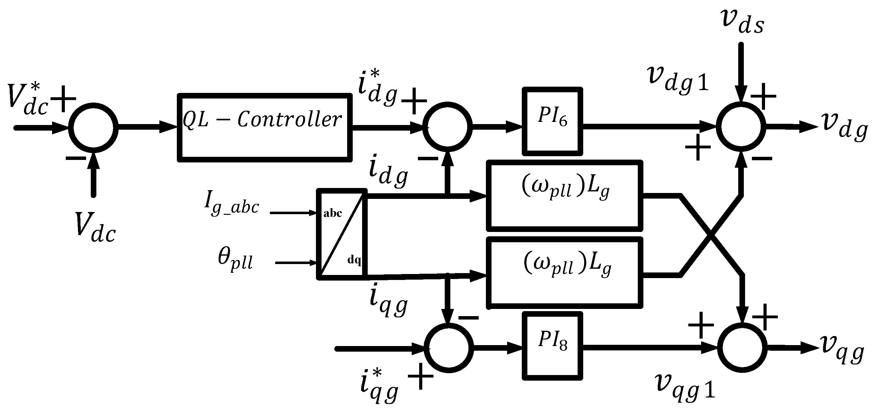
From the grid-side active ( P g c ) and reactive power ( Q g ) , the outer control loops can be designed; the obtained result will be a function of DC-link voltage v d c and the grid-side converter current i d g [7,49]. By using this, an independent control loop is developed for DC-link voltage v d c , with i d g * as its output. Similarly, the grid-side reactive power can also be controlled individually. From this outer loop, i q g * is obtained. Similarly, for the inner control loop design, the same reference frame is applied. The inner control loops are mainly designed as current control loops, which use grid-side currents as inputs. The GSC control block is given in Figure 8 [7].

4.6. Grid-Side Inner Current Control Loop

With Equations (30) and (31), the inner current control loop can be designed. In Equation (30), ω p l l L g i q g and v d s are fed as inputs at the outer end of the controller design, and in Equation (31), ω p l l L g i d g is fed at the outer end. ω p l l L g i q g and ω p l l L g i d g act as decoupling elements for the grid-side converter controller. The final obtained equations are:
v d g = R g i d g + L g p i d g
v q g = R g i q g + L g p i q g
From Equations (32) and (33), the PI controller can be designed, and it can be observed that both controllers have similar structures. Due to the very short sampling period and as the system requires a fast response rate, the controller is limited to a PI controller. Moreover, with the usage of power electronic devices and with huge variations in wind speed, which generate a lot of noise in the system, adding a derivative controller would result in an undesirable simulation result.

5. Q-Learning (QL) and Twin Delayed Deep Deterministic Policy Gradient (TD3)

Reinforcement learning (RL) algorithms are focused on goal-directed learning from iterations, which are mainly used to solve closed-loop problems. RL uses actions from learning systems that influence the later inputs [28]. An RL algorithm consists of a discrete set of environment states S , a discrete set of agent actions A , and a set of scalar reinforcement signals R . Here, the agent interacts with the environment through action, and the agent receives the current state as input; then, the agent chooses an action to generate an output. The final goal of any RL algorithm is to increase the long-run sum of values of the reinforcement signals, which can learn over time by the trial-and-error method and solve the problem [51].
The environment in reinforcement learning is fully observable and can be described as a Markov decision process (MDP), and most RL problems are formalized as MDPs. In an MDP, the action taken in the current state also affects the next state and not just the current state itself, so action plays a dominant role. Due to the action in the current state, a return reward will be assigned to the corresponding state–action pair [28].
Of the various available RL algorithms, the Q-learning algorithm is considered simple and easy to implement due to the simple way in which agents can learn and act optimally in controlled Markovian domains. The other main advantage of the Q-learning algorithm is that it is exploration-insensitive: Q values will converge to the optimal values, independently of how the agent behaves while the data are being collected [51,52]. With these advantages, this paper uses a Q-learning algorithm to train the agent to suppress oscillations and provide stable power to the grid under variable wind speeds. Assuming that the best action is taken initially, the Q-learning optimal value function is taken from [51].
Q ( s , a ) = R ( s , a ) + γ s ε S T ( s , a , s ) max Q ( s , a )
In the above equation, Q ( s , a ) is the expected discounted reinforcement of choosing action a in state s . Once the action is taken, the agent will be given a reward R for the effectiveness of the action by observing the resulting state, s , of the environment. Here, T is the probability of action a applied to state s that changes the state from s to s . For each action executed, the Q values will converge with a probability of 1 to Q * , and when the Q values are nearly converged to their optimal values, the agent will act greedily by taking the action with the highest Q value; from this greedy policy, the optimal action is determined. At any time step, there is at least one action whose estimated value is greatest or optimal; choosing the greatest value is called greedy action [28]. γ   ( 0 γ 1 ) is the discount factor, which discounts the rewards exponentially in the future [51]. Typically, an agent will look up the Q-memory lookup table, which has state s and action a and is updated as per [34,51,52]. The parameter α ( 0 α 1 ) in Equation (35) updates the Q-memory and affects the number of iterations [34].
Q ( s , a ) = ( 1 α ) . Q ( s , a ) + α ( r + γ max ( Q ( s , a ) )
Even though the Q-learning method is simple to implement, the agent cannot learn under conditions with huge variations, which is one of the observations from the current research work and a limitation of the QL agent. The other problem with the QL method is that the Q-table must be limited to certain states and actions, and the Q-table cannot be updated for a large state–action space. Therefore, the current research work explored and implemented the TD3 method so that the Q-table limitation can be overcome, and the agent can adapt to large variations in conditions.
The TD3 method is one of the model-free policy-based deep reinforcement learning algorithms built on the DDPG method [53]. The objective of the TD3 method is to increase the stability and performance by considering the function approximation error [53]. In an actor-critic setting, the learning target is:
y = r + γ Q θ ( s , π ( s ) )
where y is the learning target, r is the reward received for every action, s is the new state of the environment, γ is the discount factor, π is the optimal policy, and Q θ ( s , a ) is the function approximator with parameter θ .
The stability and performance are increased by applying three modifications [53]:
a.
Clipped double Q-learning:
In this update, the value target cannot introduce any additional overestimation using the standard Q-learning target. With a pair of actors ( π 1 , π 2 ) and critics ( Q θ 1 , Q θ 2 ) , the target update is
y 1 = r + γ m i n i = 1 , 2 Q θ ( s , π ( s ) )
In this update, the computational costs are reduced, as a single actor is optimized with respect to Q θ 1 , and the same target is used to update Q θ 2 .
b.
Target networks and delayed policy updates:
In this update, the target network is used to reduce the error over multiple updates. The policy network is updated at a lower frequency than the value network to minimize the error. The modification is made to update the policy and target networks after a fixed number of updates to the critic [53]. Thus, very few policy updates are made with this modification, and policy updates are not repeated for an unchanged critic.
c.
Target policy smoothing regularization:
In this approach, the relationship between similar actions is forced explicitly by modifying the training procedure, which is carried out by fitting the value of a small area around the target action. This will have the benefit of smoothing the value estimate by bootstrapping off a similar state-action value estimate [53]. The expectation over actions is approximated by adding a small amount of random noise to the target policy, where the noise is kept close to the original action.
The modified target update is:
y = r + γ Q θ ( s , π ( s ) ) + ϵ
ϵ ~ c l i p ( N ( 0 , σ ) , C , C )

6. Deep Reinforcement Learning-Based WECS

6.1. Design of PSS

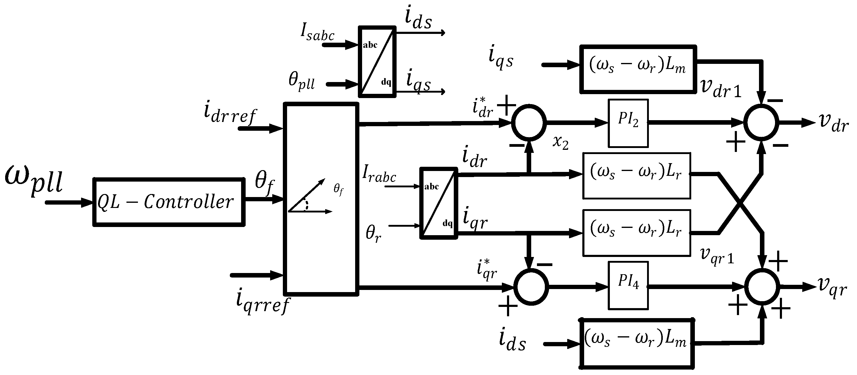
In this paper, the PSS is designed based on the transformation technique. The block diagram for the PSS with the transformation technique is shown in Figure 9.
The signal θ f is obtained from the PLL frequency ( ω p l l ):
θ f = ( K t ω p l l ) ( s T w 1 + s T w ) ( 1 1 + s T 1 )  
The transformation is defined as:
i d r * = cos ( θ f ) i d r r e f sin ( θ f ) i q r r e f
i q r * = sin ( θ f ) i d r r e f + cos ( θ f ) i q r r e f
The PSS developed with the transformation technique is implemented on the inner current controller of the RSC on both d - and q -axis control loops. The block diagram with the transformation technique is given in Figure 10.

6.2. Q-Learning Algorithm on RSC

The main motivation for using the Q-learning algorithm is to suppress low-frequency oscillations generated by variable wind speeds by searching for the best action in each state. To ensure continuous exploration and avoid tending to the local optimum, a pursuit algorithm based on the learning automata algorithm is utilized for the action policy. Initially, actions are determined with a uniform probability distribution. When the Q-table is updated, the probabilities of actions are updated as follows [54].
{ T s k + 1 ( a g ) = T s k ( a g ) + β ( 1 T s k ( a g ) ) T s k + 1 ( a ) = ( 1 β ) T s k ( a g )     a A ,   a a g T s ˜ k + 1 ( a ) = T s ˜ k ( a )   a A ,   s ˜ S ,   s ˜ s    
where T s k ( a g ) denotes the probability that an action–state pair ( a g , s ) is selected in iteration k, and β represents the action exploration rate. After the effect of this algorithm, Q k tends to Q * for a sufficiently large k , and an optimal policy is obtained. The specific Q-learning-based adaptive parameter algorithm proposed in this paper is summarized as follows:
An episode in Algorithm 1 is defined as a notion of the final time step when the agent–environment interaction breaks naturally into subsequences [28].
Algorithm 1 Q-learning-Based Adaptive Parameter in Rotor-Side Algorithm
For each episode do
     Initialize Q 0 ( x ,   a ) = 0 ,   a A ,   s S
     Initialize T x 0 ( a ) = 1 | A | ,   a A ,   s S
  For each step of episode do
       Choose a from s based on the current distribution T x ( a )
       Take action a, observe r, s
       Update Q ( x ,   a ) according to Equation (40)
    Update T x ( a ) according to Equation (43)
      s s ,   a a
  End for
End for
The damping of frequency oscillations discussed in this paper can be formulated as an MDP problem because the future state of the closed-loop controller is always dependent on the current state. Since the problems considered by reinforcement learning can be modeled as MDP models, we thus transform the adaptive parameter problem into an MDP model by designing a five-tuple ( S , A , P , γ , r ) as follows:
Design of state space S : S is a set of states that represent configurations of the system. It is assumed that all possible states are finite. To damp the low-frequency oscillations of the power system and obtain stable power output, we use active power Δ P as the state information.
The states of the MDP are described as follows: Δ P state-space (in per-unit value) is discretized into 11 spaces: ( , 0.5 ] , ( 0.5 , 0.3 ] , ( 0.3 , 0.1 ] , ( 0.1 , 0.05 ] , ( 0.05 , 0.02 ] , ( 0.02 , 0.01 ] , ( 0.01 , 0.005 ] , ( 0.005 , 0.002 ] , ( 0.002 , 0.002 ] , ( 0.002 , 0.01 ] , ( 0.01 , ) . We can see that the state distribution is unbalanced around zero, because the deviation of the active power at the rated value is also unbalanced with wind fluctuation. The QL agent is trained with 10 states and 10 action pairs. The state at iteration zero is chosen at random, and at each incremental step, the state will be in one of the intervals. Therefore, the states are divided into various sections based on the simulation results using a PSS with a PI controller, where the controlled variable is monitored. In this case, it is the active power that is a feedback parameter dependent on various other system parameters. The state space is divided into ten interval sates between an interval of -∞ to ∞. Each state consists of an interval; as the system is dynamic and continuous, the states are chosen between the intervals. The observation from the small-signal model and the simulation model with the PSS is that the change in power is within the range of −0.5 to 0.01. The intervals for each state are chosen randomly; however, the number of states is chosen based on the action.
Design of action space A : A is a set of actions that are executed by the agent to influence the environment. As mentioned before, the output of the agent should be the controller parameter at the rotor side. In this paper, we obtain the discrete action as follows: A = [−0.025 −0.02 −0.015 −0.01 −0.005 0.005 0.01 0.015 0.02 0.025]. The action space is chosen based on the output signals from the PSS controller, which are replaced by the QL agent. These are the list of actions that are provided to the agent to determine which action to choose at its corresponding state. In state 1, the action chosen can be any action and is not necessarily action 1. The Q-table, which is updated as per Algorithm 1, will choose either the action with max Q or a random Q, which is updated as per Equation (40). Even though any action can be chosen, the trained agent will use the Q values from the trained model. Therefore, under varying wind speeds, the agent will know which action to choose based on the chosen state from the updated Q values.
P : S × A   θ ( S ) is the state transition function that shows the distribution of the next state s k + 1 after executing an action a k in the environment with the current state s k . Since the parameter variation model is unknown, we can use the temporal-difference (TD) method to train the adaptive parameter policy. TD learning is a combination of Monte Carlo and dynamic programming ideas. Q-learning is an off-policy TD control algorithm [28]. In this paper, we apply a Q-learning algorithm to optimize the parameter of the rotor-side controller.
Design of reward function r ( s , a ) : r ( s , a ) is the function that maps the state–action pair ( s , a ) to a scalar, which represents the immediate reward after applying an action a to the environment with state s . In this paper, r k = k × | P P r e f | . This means that the more the active power deviates from the reference value, the smaller the immediate reward, which prompts the adjustment of the controller parameters so that the active power reaches the reference value. The parameter β used in Equation (43) is used to update the probability distribution. The value of β is 0.1. The value of α is 0.2.
The control application of QL on the RSC is employed as per Figure 11.
In Figure 11, it can be observed that the PI controller, which is developed for the PSS with the transformation technique, is completely replaced with the Q-learning algorithm.

6.3. Q-Learning Algorithm for DC-Link Voltage Control on GSC

As discussed in the above section, the primary objective of the Q-learning algorithm used is to suppress the low-frequency oscillations generated by variable wind speeds by searching for the best action in each state. On the GSC, the sensitive parameters are the DC-link voltage and grid-side current, which are observed from the small-signal model. For the action policy, a pursuit algorithm based on the learning automata algorithm is utilized. Initially, actions are determined with a uniform probability distribution. When the Q-table is updated, the probabilities of actions are updated using Equation (43). The Q-learning algorithm discussed for the RSC (Algorithm 1) is used to update the episodes on the GSC as well; the main difference is in the action and reward that are chosen for each controller. For the GSC, the action space is designed for control parameters K p 5 and K i 5 , and the reward function is defined from the DC-link voltage. The new controller design with QL on the grid-side converter is shown in Figure 12.
It can be observed that the PI controllers on the GSC are replaced with the QL algorithm. The adaptive parameter problem can be transformed into an MDP model by designing a five-tuple ( S , A , P , γ , r ) as follows:
Design of state space S : To damp low-frequency oscillations, the sensitive parameters observed from the GSC are the DC-link voltage and input reference current to the current control loop, so DC-link voltage Δ V d c is used as state information.
The states of the MDP are described as follows: On the GSC, the same state spaces defined for the RSC can be used, as the objective is to provide stable power to the grid, which is a function of active power from the RSC and GSC. In addition, the deviation of the active power at the grid-side converter is a function of V d c , which is also unbalanced with wind fluctuation. However, the action space will be completely different from the RSC action spaces, as the control parameters differ from each other.
Design of action space A : The output of the agent is a controller parameter K p 5 and K i 5 at the grid side. In this paper, we obtain the discrete action as follows:
A = [−0.19 −0.186 −0.18 −0.176 −0.172 −0.17 −0.168 −0.164 −0.16 −0.15].
The action space on the GSC is chosen based on the PI controllers, which are replaced with the QL agent. However, the state space will remain the same, as the end output is the active power, which is monitored and controlled by the agent.
P : S × A   θ ( S ) is the state transition function that shows the distribution of the next state s k + 1 after executing an action ak in the environment with the current state.
Design of reward function r ( s , a ) : In this paper, r k = k × | V d c V d c r e f | . This means that the more the grid-side active power deviates from the reference value, the smaller the immediate reward, which prompts the adjustment of the controller parameters so that the voltage reaches the reference value.
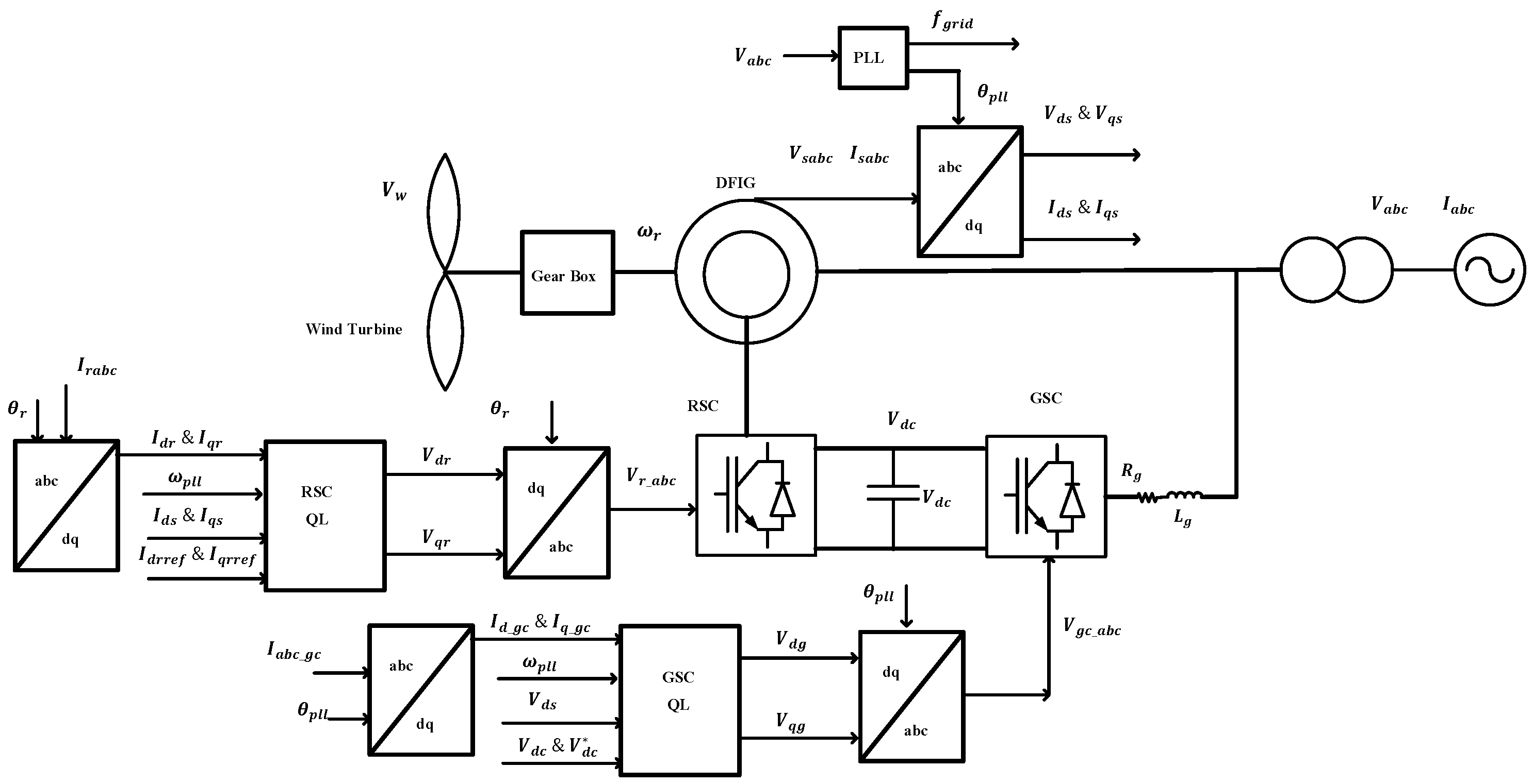
A complete block diagram with the QL-controller units discussed above can be observed in Figure 13.
In Figure 13, V w is the wind speed, ω r is the generator rotor speed, and θ r is the rotor angle, which is used for transformation from the a b c d q reference frame for rotor currents. V s a b c and I s a b c are stator voltage and currents, respectively, whereas V a b c and I a b c are grid voltage and currents, respectively. Grid voltage V a b c is provided as input to the phase-locked loop, which extracts the angle θ p l l . θ p l l is used for transformation from the a b c d q reference frame for stator voltage, stator current, grid voltage, and grid currents. In Figure 13, it can be observed that voltages fed to the rotor-side converter ( V r _ a b c ) and grid-side converter ( V g c _ a b c ) are provided by the QL controllers, which are discussed in this section.

6.4. TD3 Method

As discussed in Section 5, the TD3 method is derived from the DDPG method with a few modifications. In this section, the TD3 algorithm and its implementation are discussed. One of the objectives of this research work is to control the frequency under huge variations in speed by replacing the PI controllers, as the PI controllers cannot provide or produce satisfying tracking performance with huge variations in wind speed. Thus, the TD3 method is implemented, which provides nonlinear control. In this paper, the inner current PI controllers are completely replaced with the TD3 algorithm. The TD3 agent is implemented in an environment where the observation space is continuous or discrete, and the action space is continuous. In this experience, both the observation and action spaces are continuous. When it comes to the actor and critic, the actor is a deterministic policy actor, and the critic can be one or more Q-value function critics Q ( S , A ) . The training process consists of three steps. In step 1, the actor and critic properties are updated at each iteration by the agent. In step 2, the experience buffer is used to store past experiences. From the experience buffer, the actor and critic use a mini batch of experiences randomly. In step 3, noise is applied to the action chosen by the policy using the stochastic noise model at each episode.
TD3 implementation has four stages. In stage 1, the actor and critic functions are chosen. The actor is a deterministic actor that returns the action that maximizes the long-term reward with input with parameters θ and state S . Apart from the actor, to choose the best action, a target actor is also developed to improve the stability; the target actor parameter θ t is updated using the latest actor parameters. There are two critics: one is the value critic, and the second critic is the target critic. The value critic takes state S and action A as inputs and provides the expectation of the long-term reward. The target critic is responsible for improving the stability of the optimization. Target critic parameters are updated using the latest critic parameter values. In stage 2, the agent is created with the state and action specifications of the environment. As the agent has both actor and critic networks in the environment, in stage 3, the agent is now trained to learn and update the actor and critic models at each episode. Training is implemented as per Algorithm 2 [53]. In stage 4, the target actor and the target critic parameters are updated using one of the target update methods, such as periodic, smoothing, and periodic smoothing. However, for this research work, the smoothing update is chosen.
Algorithm 2 TD3 [53]
Initialize critic networks Q 1 , Q 2 with random parameters 1
Initialize target critic with same random parameters 2 ; so 1 = 2
Initialize actor network π θ with random parameters θ 1 , θ 2
Initialize target actor network π θ with same random parameters θ 2
So, for target networks θ 1 θ 1 ,   θ 2 θ 2 ,
Initialize replay buffer β
For t = 1 to T do
    For current state of observation S , select action with exploration noise a ~ π ( s ) + ε ,   ~ N ( 0 , σ ) . Here, is the stochastic noise from the noise model
Execute action and observe reward r and new state s .
Store the experience ( s , a , r , s ) in β (experience buffer)
Sample a random mini batch of   N transitions ( s , a , r , s ) from β
If s is a terminal state, set the value function target y i = r ; else
      a ˜ π ( s ) + ϵ ,   ϵ ~   c l i p ( N ( 0 , σ ) ,   C , C )
        y   r + γ m i n i = 1 , 2 Q θ ( s , a ˜ )  
Update critics θ i   a r g m i n θ i N 1   ( y Q θ i ( s , a ) ) 2
If t mod d then
    Update   by deterministic policy gradient:
         J ( ) = N 1 a Q θ 1 ( s , a ) | a = π ( s ) π ( s )
   Update target networks (smoothing):
    θ i τ θ i + ( 1 τ ) θ i
    τ + ( 1 τ )
end if
end for
In the current work, the inner current controller on the rotor-side controller is replaced with the TD3 agent. Therefore, the inputs for the TD3 agent are f ( i d r , i q r , i d r _ r e f , i q r _ r e f , ω r , ω r _ r e f ) . Here, i d r , i q r are rotor-side currents, and i d r _ r e f , i q r _ r e f are the outputs of the outer current control loop on the RSC. ω r and ω r _ r e f are the rotor speed and reference speed, respectively. Both the current and speed with their references are provided as inputs or are used as the parameters for observation. The reward is computed by taking the error between the reference values and the actual values of currents. The reward R is computed as shown in Equation (44).
R t = ( Q 1 ( i d r i d r r e f ) 2 + Q 2 ( i q r i q r r e f ) 2 + R ( a t 1 j ) 2 ) 100 d  
Therefore, the number of observations is six, which are the inputs to the TD3 agent, and the number of actions is two, v d r and v q r . As we have the observations and action space available, the next step is to create the agent block, as shown in Figure 14.
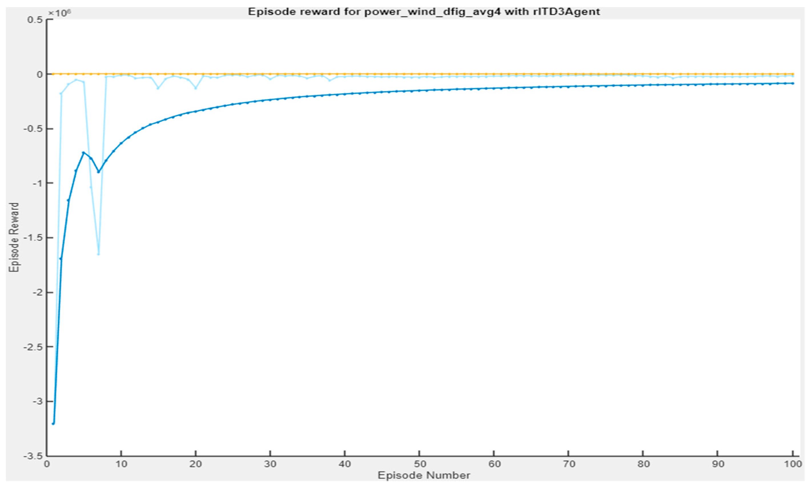
For the TD3 agent, two critic networks are created with a deep neural network with state and action as inputs and one output. The neural network developed is a fully connected layer for both state and action paths. In the same way, for both actor networks, fully connected layers are used. The TD3 agent will determine the action that needs to be taken for the given state. To train the agent, the TD3 agent is provided with its discount factor, the buffer length, mini-batch size, target smoothing factor, and finally, the target update frequency. For training, the agent is allowed to run each training for 1000 episodes and stop training when the agent receives a cumulative average reward ≥ −200 over 100 consecutive episodes. Training progress with the TD3 agent is shown in Figure 15, which shows that the average reward of each episode increases, and the policy becomes stable after 40 episodes. The training process was executed for a duration of 32 h, as it reached the specified maximum episode numbers. In Figure 15, the thick blue line represents the average reward, and the light blue line indicates the episode reward and the yellow line shows the episode Q 0 .

7. Results and Discussion

7.1. Simulation Results with the Newly Designed PSS

The model discussed in this paper was built in MATLAB/Simulink. The topology is shown in Figure 13. There have been extensive works published based on simulations [4,10,35,55]. A small-signal model was developed to identify the state variables that affect the stability of the overall system. From the small-signal model, the sensitive variables observed are i d r , i q r , i q s , x 7 , v d s , and θ p l l . The input given to the power system stabilizer is the frequency ω p l l . One of the main observations from small-signal stability analysis is that the state variables associated with the inner current control loop tend to move faster towards the real axis, making the system unstable. This is observed with the large-signal model as well when applying small faults. The performance evaluation of the system with a PSS and without a PSS can be observed from the small-signal model. The low-frequency mode of the system can be observed from the same small-signal model. Usage of the eigenvalue distribution of systems with and without a PSS to identify the ultra-low-frequency oscillation mode can be observed in [36]. The shift of eigenvalues with the new PSS implemented is noted in Table 1 below. The eigenvalues of ( E , A ) x 1   and   θ f are newly added signal inputs from the PSS. The time constants for the washout filter and compensator are determined from the small-signal model by observing the stability of the system. V d c and x 5 are the signal inputs of the outer current control loop of the grid-side converter. x 2 and x 4 are the input signals to the PI controllers ( P I 2   and   P I 4 ) at the inner current control loop of the RSC. x 7 is the input signal to the PI controller ( P I 7 ) at the inner current control loop of the GSC. Controller data, DFIG, and the complete system parameters are presented in Appendix A.
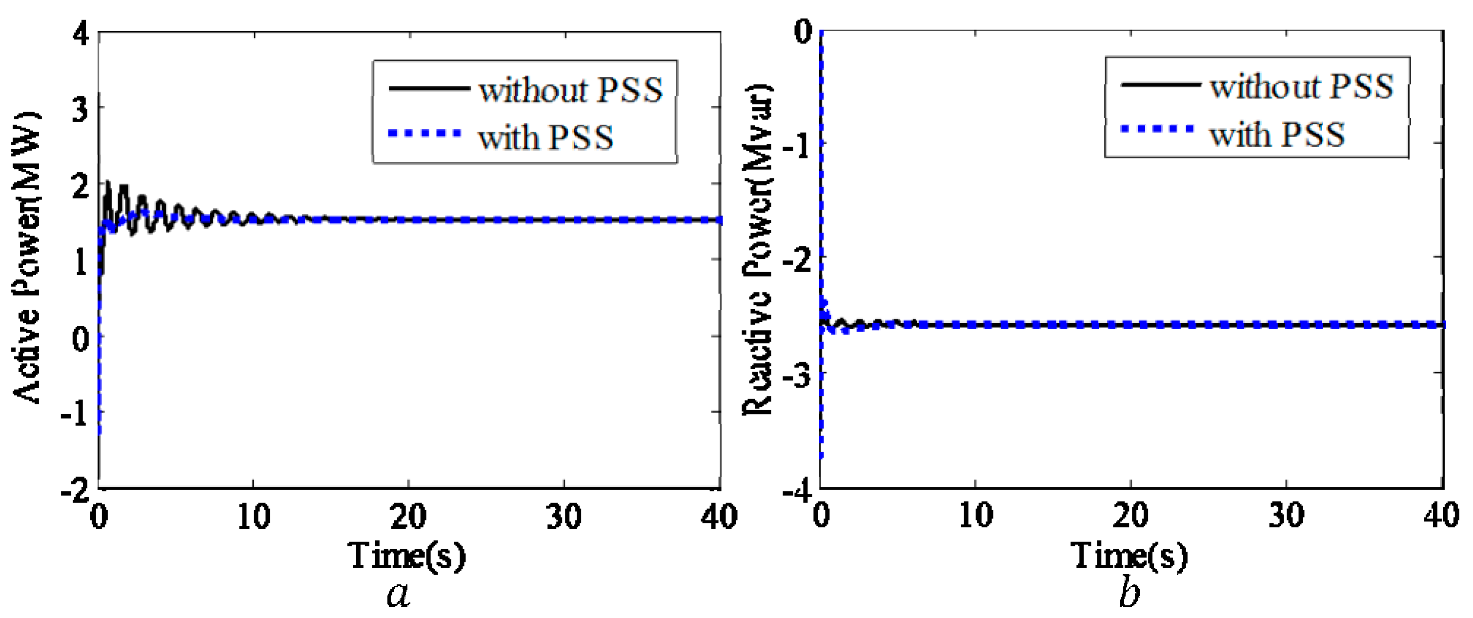
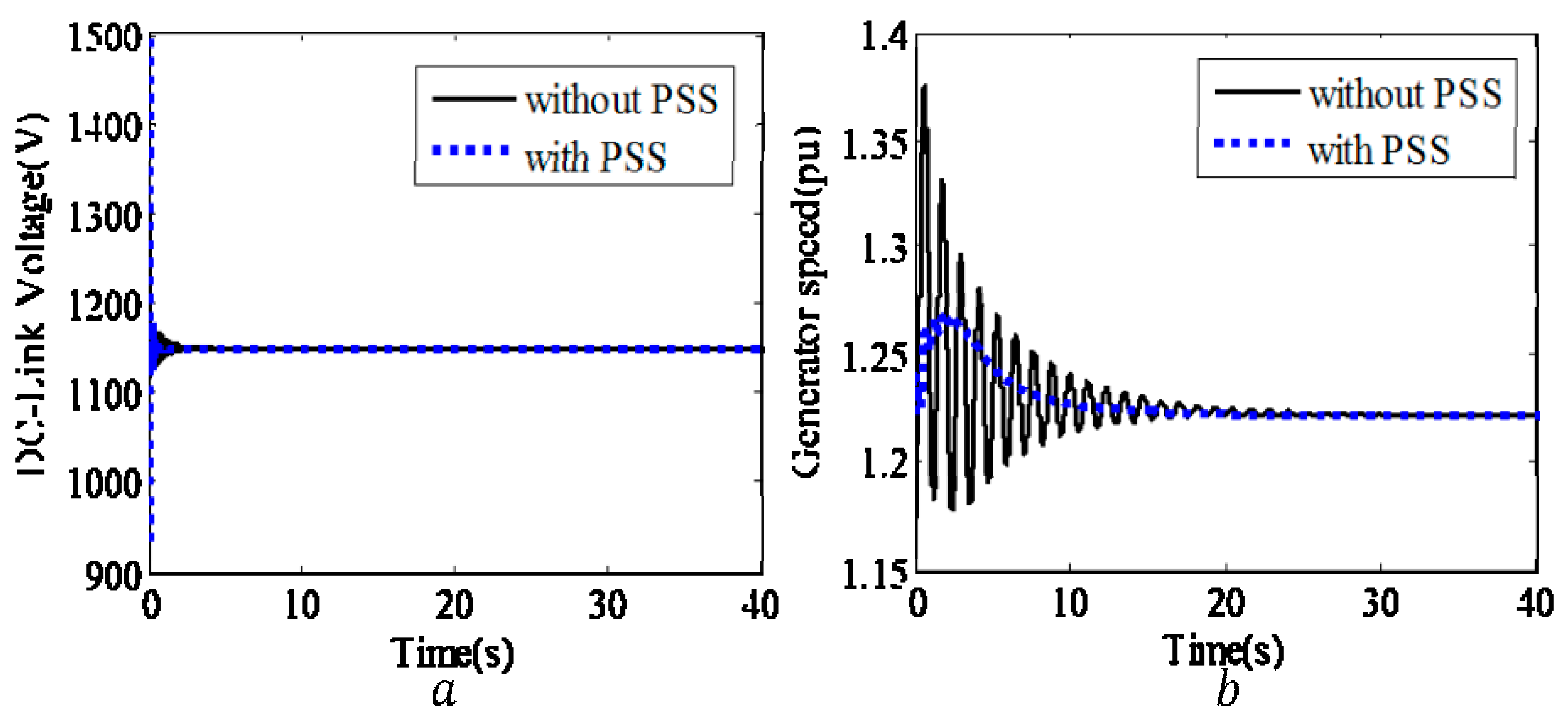
The results for the power system stabilizer with the transformation technique are shown below in Figure 16.
From Figure 16 and Figure 17, it can be observed that there is an increase in the damping of the oscillations for both active power and generator speed with the PSS implemented with the transformation technique.

7.2. Fault Analysis with Transformation PSS

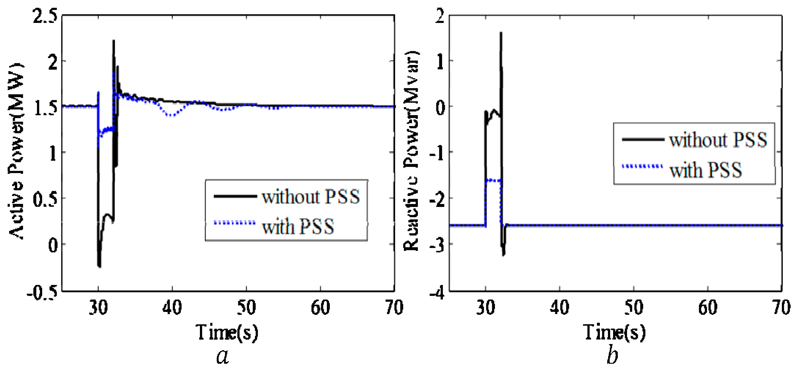
The plot of the transformation PSS during the fault condition is shown below. It can be observed that the oscillations are damped even during the fault condition. This can be more clearly observed from the power plot, in which the oscillations are damped, and the settling time is also much less. From this discussion, it can be concluded that the PSS is working effectively during the fault condition.
For fault analysis, a three-phase fault was applied to the system for a time of τ = 2 s between times τ = 30 s and τ = 32 s. The results obtained for active power and reactive power are shown in Figure 18a,b, respectively. In the above plot, it can be observed that the PSS with voltage as input is able to damp the oscillations during the fault, and the settling time after the fault is also much less.
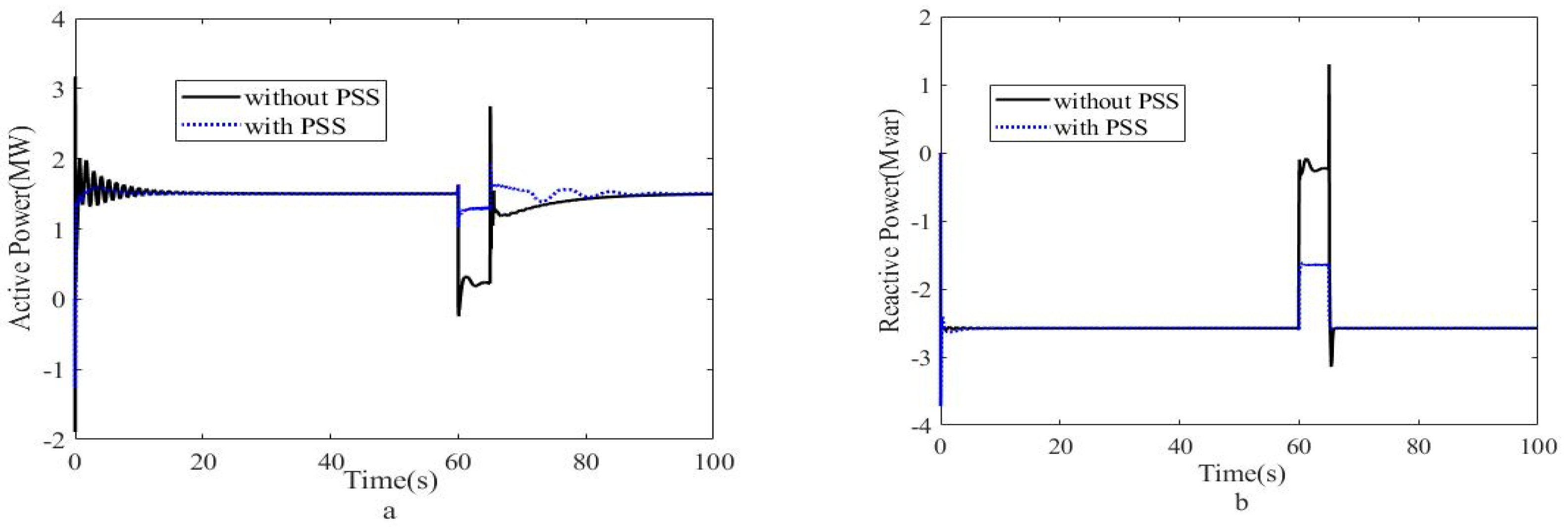
Figure 19 provides the simulation results for the system during a single-phase short circuit fault. The fault was applied to the system for τ = 5 s between times τ = 60 s and τ = 65 s. It can be observed that the PSS is able to damp the oscillations.

7.3. Results with Q-Learning Algorithm

Next, a Q-learning algorithm was implemented on the developed PSS at the RSC and the outer current control loop of the GSC with a variable wind speed. The algorithm model was applied at P s r e f and V d c r e f . Since the control objective is to stabilize the output of the power system with active and reactive power without low-frequency oscillations, this paper uses parameters that are directly related to the active power change in the power system as the state of the agent and the control output of the controller as the action of the agent to train the appropriate control strategy. After testing, when the wind speed fluctuates in a small range, it is easier to stabilize the system through the reinforcement learning controller. Therefore, the wind speed of this experiment was designed to be between 14 m/s and 15 m/s.
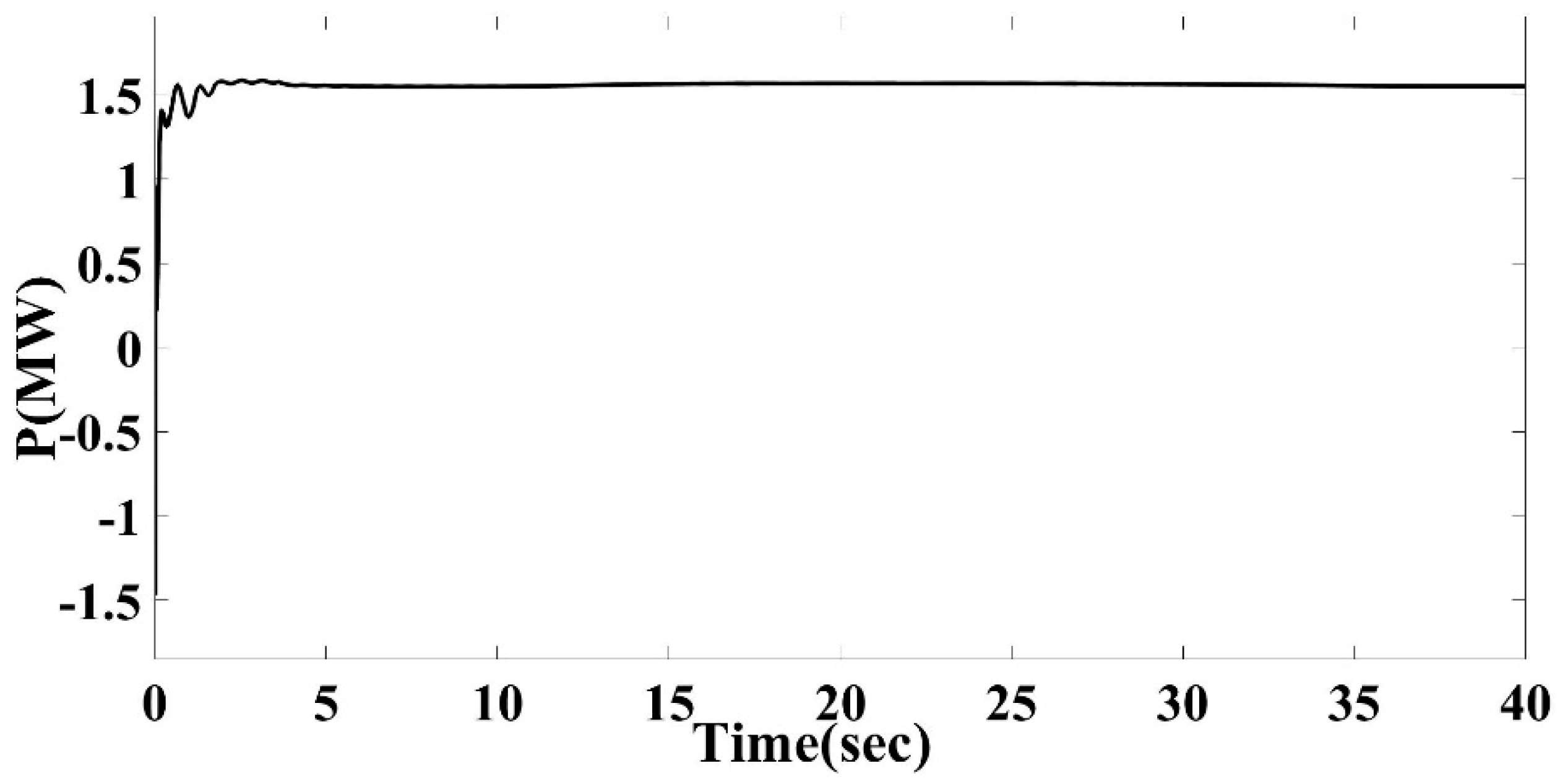
The following is the output waveform of the active power of the power system after several iterations of the reinforcement learning controller. The active power waveform is observed at iteration 18, which can be observed in Figure 20.
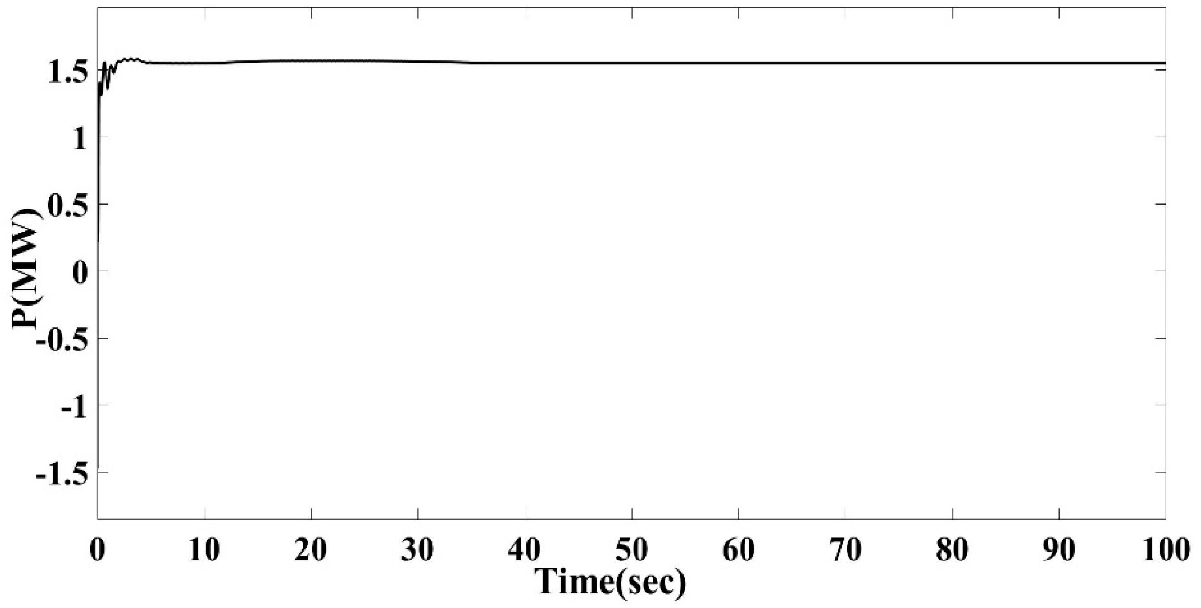
In Figure 20, it can be observed that the generated power tends to be smooth without any oscillations, which indicates that the QL algorithms implemented were able to learn from the system and provide the desired output.
However, the final active power is still not smooth. Next, the system was iterated until the desired active power was generated without any oscillations, which was observed at the 21st iteration. Figure 21 shows the response of the active power at the 25th iteration. After this point, the system response will not differ, as the Q-learning agent is able to learn about the system in various states and provide the required action at different states. In Figure 20, Figure 21, Figure 22, Figure 23 and Figure 24, it is observed that under the action of the trained reinforcement learning controller, the system can output stable active power without low-frequency oscillations. The total time taken for 25 episodes or iterations is 90 min.
Figure 22 shows the control of reactive power at the 25th iteration. It can be observed that the QL agent is able to learn from the environment and control reactive power as well.
The output speed and power as the wind speed changes are plotted in Figure 23. As can be seen in Figure 23a, when the wind speed changes, the speed and active power of the power system are stabilized.

7.4. Comparing Q-Learning Algorithm with PI Controllers

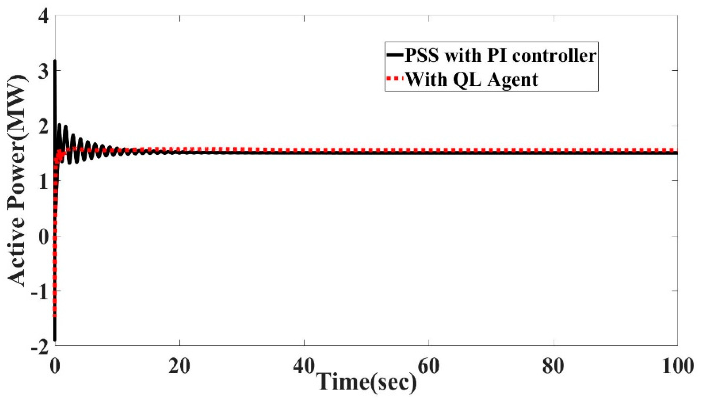
The Q-learning algorithm developed completely replaces the PI controllers both on the RSC and GSC and the power system stabilizer at the RSC. From the results, it is observed that the model-free algorithm can learn from the system environment and generate similar results to those of the PI controller.
In Figure 24, the dotted red line indicates the curve for active power with the QL algorithm, and the continuous curve shows the active power with PI controllers. It can be observed that the Q-learning algorithm controls the active power similarly to the PI controller. The advantage of the developed Q-learning model over the PI controller design is that the Q-learning agent provides the controller parameters dynamically, whereas the gains in the PI controller are fixed; moreover, the Q-learning algorithm is implemented with varying wind speeds, whereas the PI controller is implemented with a constant wind speed. Figure 25 shows a comparison of the reactive power for the developed PSS with the PI controller and Q-learning algorithm.

7.5. Comparing Q-Learning Algorithm with PI Controllers under Fault Conditions

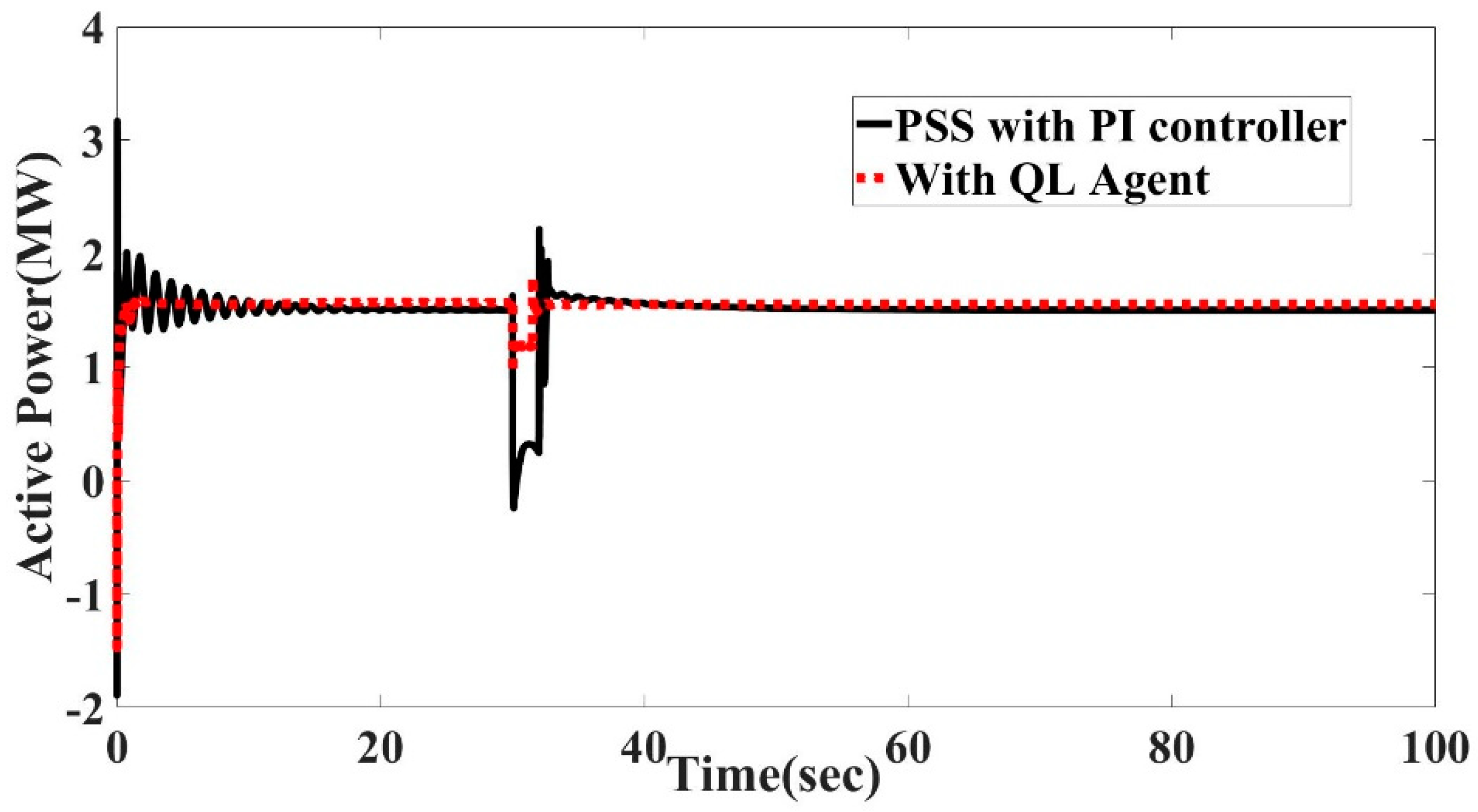
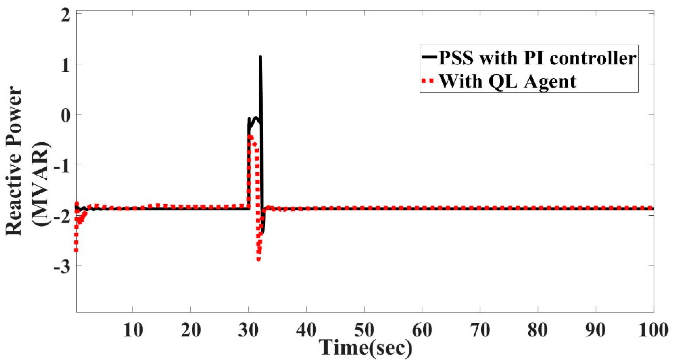
To evaluate the control of the Q-learning algorithm under fault conditions, a three-phase fault was employed at the grid end before the transformer. The clearing time was 2 s, starting at 30 s and clearing at 32 s. Figure 26 and Figure 27 show the active power and reactive power plots, respectively, under fault conditions. In Figure 26, the red dotted line is the active power with the Q-learning algorithm, and the continuous line shows the curve for the PI controller. It can be observed that the damping of oscillations is more effective with the Q-learning algorithm when compared to the PSS with PI controllers.
In Figure 27, the red dotted curve indicates the reactive power with the Q-learning algorithm, and the continuous curve is with the PI controller. In the figure, it can be observed that the damping of oscillations is more effective with the Q-learning algorithm when compared with the PI controllers.
The proposed Q-learning algorithm can be compared with the PSS using the Q-learning algorithm from [35]. In [35], the case study used is a four-machine two-area system where a Q-learning-based PSS is employed to damp the frequency oscillations. The same can be observed in the current paper; however, the systems used are completely different. Moreover, in the current paper, the performance of Q-learning is observed under fault conditions as well. In Figure 24, Figure 25, Figure 26 and Figure 27, a clear comparison can be observed between the PSS with the PI controller and Q-learning. Here, the PSS with the PI controller can be treated as a test case to evaluate the performance of the Q-learning-based model. In Figure 24, Figure 25, Figure 26 and Figure 27, the proposed Q-learning-based model reaches the steady state in a shorter time compared with the classical PI controller-based PSS.

7.6. Comparing TD3 Agent with Q-Learning Algorithm

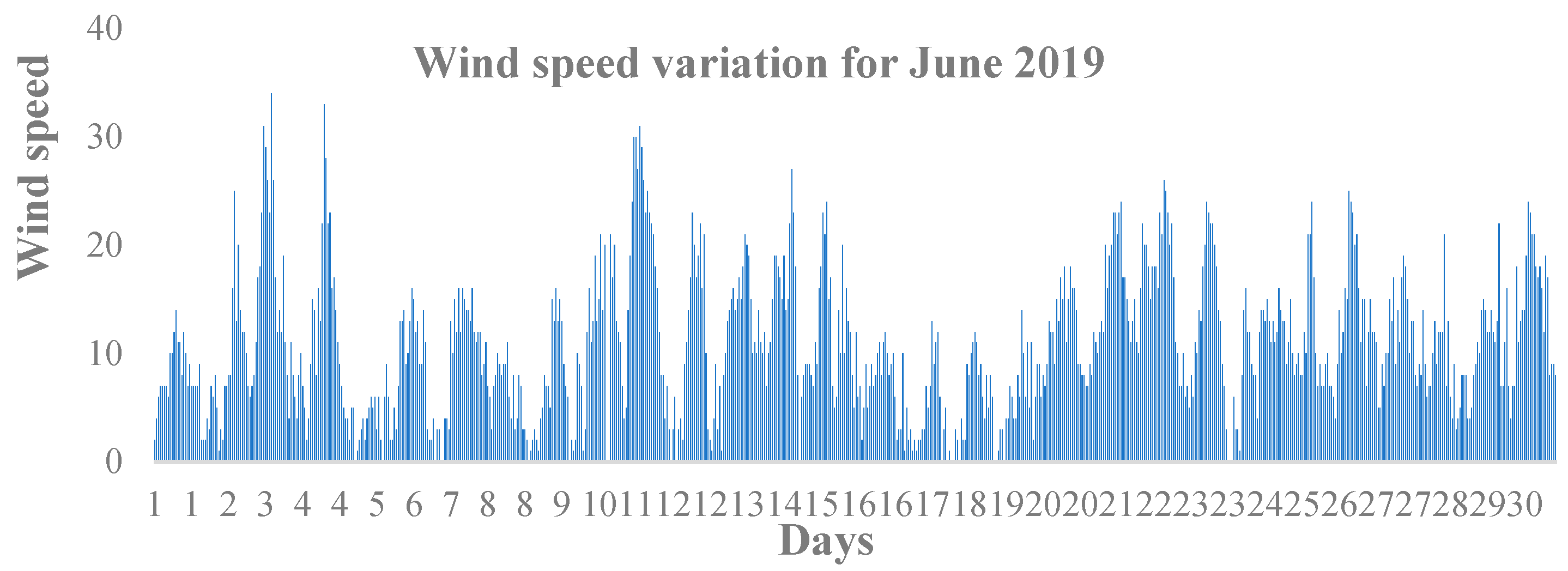
Simulations were carried out with large variations in wind speed using PI, Q-learning, and the TD3 agent. The wind speeds used are from the Ottawa region for the whole month of June 2019.
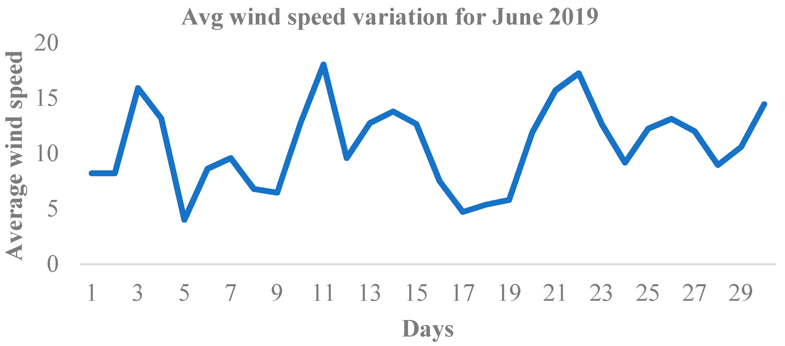
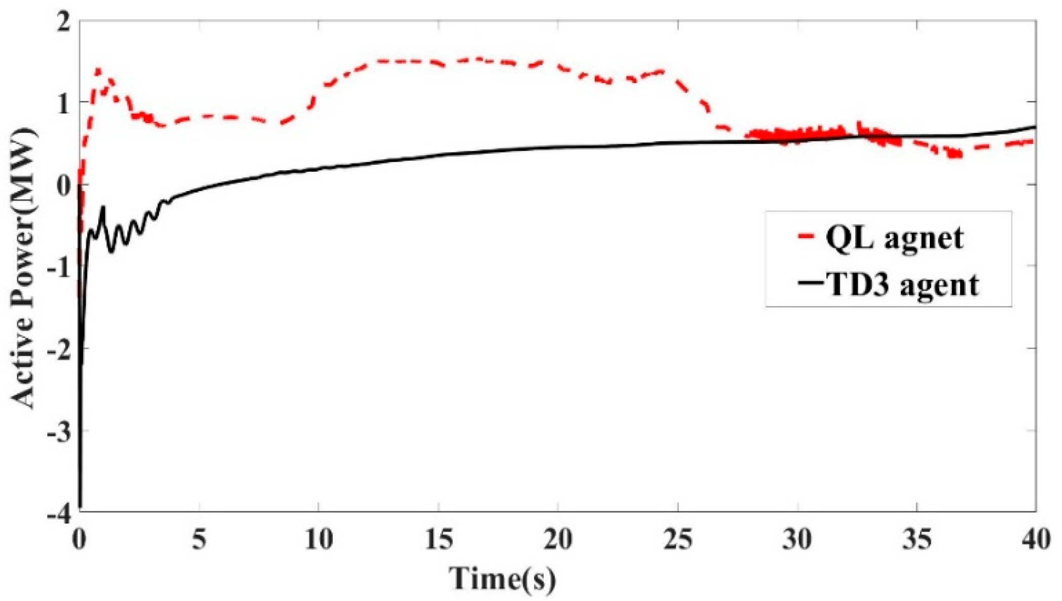
The wind speed variation shown in Figure 28 was used as an input to the DFIG WECS. With varying wind speeds, it is hard for the regular PI controller to maintain the frequency and, at the same time, provide a table output to the grid. The average wind speed variations can be observed in Figure 29. The active power and reactive power with the PSS with QL vs. the PSS with the TD3 agent can be seen in Figure 30 and Figure 31, respectively. It can be observed that both active power and reactive power are not stable with such huge wind speed variations in either the PSS with the PI controller or the Q-learning agent. However, once the TD3 agent implemented on the inner current control loop of the RSC learns the system dynamics, the agent can control the generator speed and inner currents with respect to their reference values. Therefore, with large variations in wind speed and without using an inner PI controller, with the TD3 agent, the system can produce stable active and reactive power with varying wind speeds by mitigating lower frequencies. The system with the PI controller does not even respond to large variations in wind speed, as it can work only for a constant wind speed.
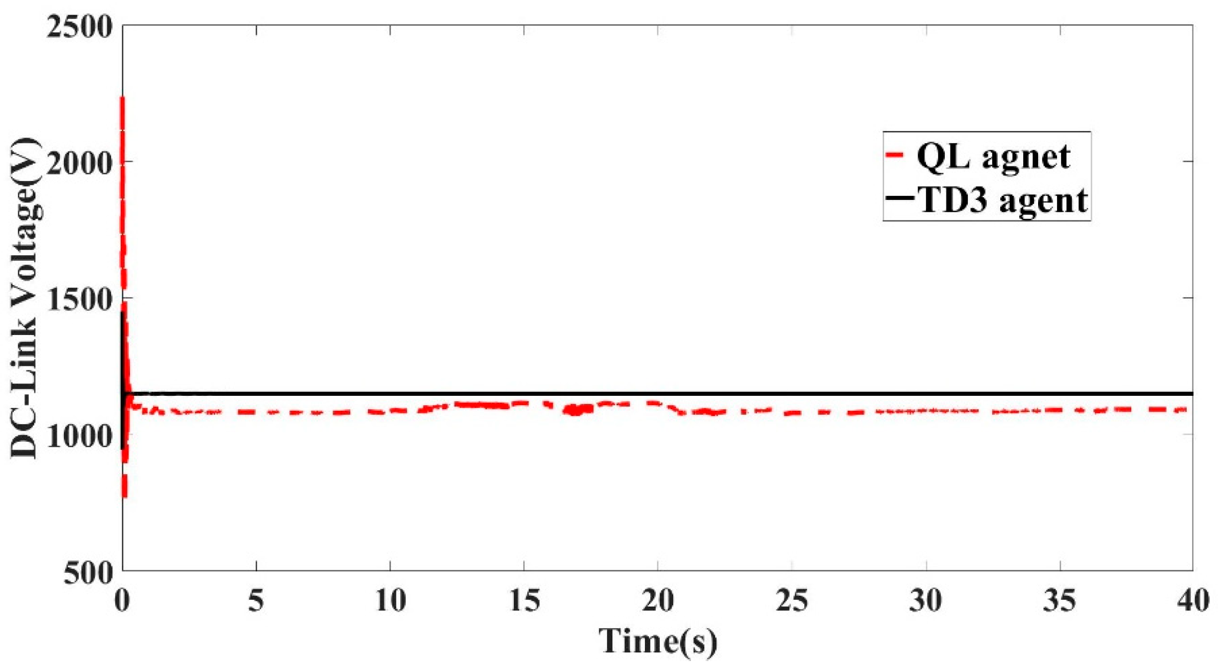
Figure 32 and Figure 33 show the DC-link voltage and generator speed comparison between the QL agent and TD3 agent. In the figures, it can be observed that the TD3 agent can learn and control the system under large variations in wind speed and performs better than the QL agent.

8. Limitation and Future Work

The wind DFIG system with the PSS and PI controllers works fine for a constant speed, which is observed under normal and fault conditions. If a varying wind speed is provided, then the PSS cannot suppress any oscillations, and the system is very unstable. The PSS with the PI controller cannot be adopted or used for large variations in wind speed. To overcome the limitation of varying wind speeds, reinforcement learning is used to learn the system dynamics and mitigate oscillations. For this, first, the PSS and the PI controllers from both the RSC and GSC are replaced with the QL agent. The Q-learning algorithm developed in this paper is implemented for a very small range of varying wind speeds and does not respond accurately for large variations in wind speed. The observation is that the QL agent is not successful in learning the system dynamics with huge variations in wind speed. To overcome the limitation of the application of an RL to large variations in wind speed, advanced RL techniques such as actor-critic (A2C or A3C) or policy gradient methods such as Deep Deterministic Policy Gradient (DDPG) will be helpful, as these methods are robust in learning about the environment. To handle large variations in wind speed, the TD3 method is introduced in this research. Usage of the A3C-based strategy can be observed in [36], where the PSS parameters were tuned to suppress low-frequency oscillations for a 10-machine 39-bus transmission network. Thus, A2C or A3C can be adopted to suppress low-frequency oscillations for large variations in wind speed in DFIG-based WECS. As discussed at the beginning of Section 7, the complete model was built in the MATLAB/Simulink environment. For this research work, there was no experimental hardware involved. The complete results and comparisons are discussed in Section 7.

9. Conclusions

In this work, a DFIG-equipped WECS was developed, and closed-loop controllers were designed to damp the oscillations by controlling both active and reactive power. First, a small-signal model was developed to identify the sensitive parameters that affect the stability of the system, and from the SS model, the proportional and integral gains were derived. The derived PI gains were used in the inner current control loops of the large-signal model. Next, the PI controllers were completely replaced with the Q-learning-based RL technique. The Q-learning-based model-free power system stabilizer and DC-link voltage regulator were developed on both the rotor side controller and grid side controller. From the results, it is observed that the designed model-free PSS can damp the oscillations under small wind speed variations and faulty conditions. The conclusion is that the QL algorithm agent can learn from the environment and control the active power by helping the system to operate under normal conditions with variable wind speeds by making the system model-free. However, the limitation of the QL method is that it cannot control under large variations in wind speed. To overcome this limitation, an actor-critic method called the TD3 method is introduced. From the results, it can be observed that the TD3 agent can learn the system dynamics under large variations in wind speed, and the agent can deliver the desired active and reactive power to the grid.

Author Contributions

Conceptualization, R.K. and S.L.; methodology, R.K. and S.L.; Software R.K.; Validation R.K., S.L. and W.S.; formal analysis R.K. and S.L.; investigation R.K.; data curation R.K. and S.L.; writing—original draft preparation R.K.; writing—review and editing, R.K, S.L. and W.S.; visualization, R.K.; supervision, S.L. and W.S.; funding acquisition, S.L. All authors have read and agreed to the published version of the manuscript.

Funding

This research was funded by Natural Sciences and Engineering Research Council of Canada, Discovery Grant.

Institutional Review Board Statement

Not applicable.

Informed Consent Statement

Not applicable.

Data Availability Statement

The data presented in this study are available on request from the corresponding author.

Conflicts of Interest

The authors declare no conflict of interest.

Appendix A. Parameters for the System

Base Quantities:
S b a s e = 1.5 ;   ( MVA ) Generator rated power
V b a s e = 120 2 ;   ( V ) Stator rated voltage
ω b a s e = 2 p i 60 ;   ( rad / s ) Electrical base speed
I b a s e = ( 2 3 ) ( S b a s e V b a s e ) ;   ( A ) Base current
Z b a s e = ( V b a s e I b a s e ) ;   ( Ω ) Base impedance
L b a s e = ( Z b a s e ω b a s e ) ;   ( H ) Base inductance
Ψ b a s e = L b a s e I b a s e ; ( w b t u r n s ) Base flux
P b a s e , Q b a s e = S b a s e ;   ( W ) ,   ( VAr ) Base active and reactive power
DFIG Parameters:
ω s = 1   [ pu ] Synchronous speed
r s = 0.00706   [ pu ] Stator resistance
r r = 0.005   [ pu ] Rotor resistance
L l s = 0.171   [ pu ] Stator inductance
L l r = 0.156   [ pu ] Rotor inductance
L m = 2.9   [ pu ] Mutual inductance
H g = 0.9   s Generator inertia constant
p = 3 No. of pairs of poles
Drivetrain data:
H t = 4.32   s Wind turbine inertia constant
K t g = 1.11 Shaft spring constant
D t g = 1.5 Shaft mutual damping
V w = 15   [ m / s ] rated wind speed
R = 33.3 Blade length
ρ = 1.225 [ kg / m 3 ] Air density
ω t r a t e d = V w r a t e d λ o p t i m a l R   [ rad / s ] Turbine rated speed
λ o p t i m a l = 9.94 Tip speed ratio
C p m a x = 0.5 Maximum value of C p
C 1 = 0.645 ; C 2 = 116 ; C 3 = 0.4 ; C 4 = 5 ; C 5 = 21 ; C 6 = 0.009 ; C 7 = 0.08 ; C 8 = 0.35 ;
DC-Link:
C = 10000 E 6   [ Frads ]
V d c n o m i n a l = 1150   [ V ]
Controller data:
Rotor-side converter controller:
K p 1 = 1.25 ;   K i 1 = 300 Active power loop
K p 2 = 0.6 ;   K i 2 = 8 Inner current controller loop ( d - axis )
K p 3 = 1.25 ;   K i 3 = 300 Stator reactive power loop
K p 4 = 0.6 ;   K i 4 = 8 Inner current controller loop ( q - axis )
Grid-side converter controller:
K p 5 = 8 ;   K i 5 = 400 DC-link controller
K p 6 = 0.83 ;   K i 6 = 5 Inner current controller loop ( d - axis )
K p 7 = 1.25 ;   K i 7 = 300 Grid-side reactive power controller
K p 8 = 0.83 ;   K i 8 = 5 Inner current controller loop ( q - axis )
PLL:
K p p l l = 50 ;   K i p l l = 5 00
Reference values:
Q s r e f = Q g r e f = 0 Reactive power reference values
V d c r e f = V d c n o m i n a l
PSS with voltage as input:
K p = 5 ; T w = T 1 = 1
PSS with frequency as input (transformation technique):
K f = 10 ;
T w = 2 ; and T 1 = 1 .
Pitch controller:
K p p = 150 ; K p c = 3 ; K i c = 30 ,   θ m a x = 27 ; θ m i n = 0

References

  1. Ellis, A.; Muljadi, E. Wind Power Plant Representation in Large-Scale Power Flow Simulations in WECC. In Proceedings of the 2008 IEEE Power and Energy Society General Meeting—Conversion and Delivery of Electrical Energy in the 21st Century, Pittsburgh, PA, USA, 20–24 July 2008; pp. 1–6. [Google Scholar] [CrossRef]
  2. Zobaa, A.F.; Bansal, R.C. Handbook of Renewable Energy Technology; World Scientific: Singapore, 2011; ISBN 978-981-4289-06-1. [Google Scholar]
  3. Nayar, C.V.; Islam, S.M.; Dehbonei, H.; Tan, K.; Sharma, H. Chapter 1—Power Electronics for Renewable Energy Sources. In Alternative Energy in Power Electronics; Rashid, M.H., Ed.; Butterworth-Heinemann: Oxford, UK, 2011; pp. 1–79. [Google Scholar]
  4. Zhou, F.; Liu, J. A Robust Control Strategy Research on PMSG-Based WECS Considering the Uncertainties. IEEE Access 2018, 6, 51951–51963. [Google Scholar] [CrossRef]
  5. Shang, L.; Hu, J. Sliding-Mode-Based Direct Power Control of Grid-Connected Wind-Turbine-Driven Doubly Fed Induction Generators under Unbalanced Grid Voltage Conditions. IEEE Trans. Energy Convers. 2012, 27, 362–373. [Google Scholar] [CrossRef]
  6. Zeng, H.; Zhu, Y.; Liu, J. Verification of DFIG and PMSG Wind Turbines’ LVRT Characteristics through Field Testing. In Proceedings of the 2012 IEEE International Conference on Power System Technology (POWERCON), Auckland, New Zealand, 30 October–2 November 2012; pp. 1–6. [Google Scholar]
  7. Qiao, W. Dynamic Modeling and Control of Doubly Fed Induction Generators Driven by Wind Turbines. In Proceedings of the 2009 IEEE/PES Power Systems Conference and Exposition, Seattle, WA, USA, 15–18 March 2009; pp. 1–8. [Google Scholar]
  8. Bevrani, H.; Watanabe, M.; Mitani, Y. Power System Monitoring and Control; Wiley: Hoboken, NJ, USA, 2014; ISBN 978-1-118-85247-7. [Google Scholar]
  9. Vassell, G.S. Northeast Blackout of 1965. IEEE Power Eng. Rev. 1991, 11, 4. [Google Scholar] [CrossRef]
  10. Dehghani, M.; Han, W.; Karimipour, H. Coordinated Fuzzy Controller for Dynamic Stability Improvement in Multi-Machine Power System. In Proceedings of the 2018 IEEE International Conference on Smart Energy Grid Engineering (SEGE), Oshawa, ON, Canada, 12–15 August 2018; pp. 165–170. [Google Scholar]
  11. Anaya-Lara, O. Power System Stabiliser for a Generic DFIG-Based Wind Turbine Controller. In Proceedings of the 8th IEE International Conference on AC and DC Power Transmission (ACDC 2006), London, UK, 28–31 March 2006; Volume 2006, pp. 145–149. [Google Scholar]
  12. Hughes, F.M.; Anaya-Lara, O.; Jenkins, N.; Strbac, G. Control of DFIG-Based Wind Generation for Power Network Support. IEEE Trans. Power Syst. 2005, 20, 1958–1966. [Google Scholar] [CrossRef]
  13. Hughes, F.M.; Anaya-Lara, O.; Jenkins, N.; Strbac, G. A Power System Stabilizer for DFIG-Based Wind Generation. IEEE Trans. Power Syst. 2006, 21, 763–772. [Google Scholar] [CrossRef]
  14. Hughes, F.M.; Anaya-Lara, O.; Ramtharan, G.; Jenkins, N.; Strbac, G. Influence of Tower Shadow and Wind Turbulence on the Performance of Power System Stabilizers for DFIG-Based Wind Farms. IEEE Trans. Energy Convers. 2008, 23, 519–528. [Google Scholar] [CrossRef]
  15. Mishra, Y.; Mishra, S.; Li, F.; Dong, Z.Y.; Bansal, R.C. Small-Signal Stability Analysis of a DFIG-Based Wind Power System under Different Modes of Operation. IEEE Trans. Energy Convers. 2009, 24, 972–982. [Google Scholar] [CrossRef]
  16. Mishra, Y.; Mishra, S.; Tripathy, M.; Senroy, N.; Dong, Z.Y. Improving Stability of a DFIG-Based Wind Power System With Tuned Damping Controller. IEEE Trans. Energy Convers. 2009, 24, 650–660. [Google Scholar] [CrossRef]
  17. Surinkaew, T.; Ngamroo, I. Coordinated Robust Control of DFIG Wind Turbine and PSS for Stabilization of Power Oscillations Considering System Uncertainties. IEEE Trans. Sustain. Energy 2014, 5, 823–833. [Google Scholar] [CrossRef]
  18. Iswadi, H.R.; Morrow, D.J.; Best, R.J. Small Signal Stability Performance of Power System during High Penetration of Wind Generation. In Proceedings of the 2014 49th International Universities Power Engineering Conference (UPEC), Cluj-Napoca, Romania, 2–5 September 2014; pp. 1–6. [Google Scholar]
  19. Mendonca, A.; Lopes, J.A.P. Simultaneous Tuning of Power System Stabilizers Installed in DFIG-Based Wind Generation. In Proceedings of the 2007 IEEE Lausanne Power Tech, Lausanne, Switzerland, 1–5 July 2007; pp. 219–224. [Google Scholar]
  20. Elkington, K.; Ghandhari, M.; Söder, L. Using Power System Stabilisers in Doubly Fed Induction Generators. In Proceedings of the Australasian Universities Power Engineering Conference, Sydney, NSW, Australia, 14–17 December 2008; p. 6. [Google Scholar]
  21. Ke, D.P.; Chung, C.Y.; Xue, Y. Controller Design for DFIG-Based Wind Power Generation to Damp Interarea Oscillation. In Proceedings of the 2010 5th International Conference on Critical Infrastructure (CRIS), Beijing, China, 20–22 September 2010; pp. 1–6. [Google Scholar]
  22. Gong, B.; Xu, D.; Wu, B. Network Damping Capability of DFIG-Based Wind Farm. In Proceedings of the 2010 IEEE Energy Conversion Congress and Exposition, Atlanta, GA, USA, 12–16 September 2010; pp. 4083–4090. [Google Scholar]
  23. Zhang, Y.; Chen, G.P.; Malik, O.P.; Hope, G.S. An Artificial Neural Network Based Adaptive Power System Stabilizer. IEEE Trans. Energy Convers. 1993, 8, 71–77. [Google Scholar] [CrossRef]
  24. Kahouli, O.; Alshammari, B.; Dhouib, B. Application of ANN and ANFIS Techniques for PSS Tuning in a Multimachine Power System. In Proceedings of the 2019 16th International Multi-Conference on Systems, Signals & Devices (SSD), Istanbul, Turkey, 21–24 March 2019; pp. 435–440. [Google Scholar]
  25. Hariri, A.; Malik, O.P. A Fuzzy Logic Based Power System Stabilizer with Learning Ability. IEEE Trans. Energy Convers. 1996, 11, 721–727. [Google Scholar] [CrossRef]
  26. Chaturvedi, D.K.; Malik, O.P. Neurofuzzy Power System Stabilizer. IEEE Trans. Energy Convers. 2008, 23, 887–894. [Google Scholar] [CrossRef]
  27. Boonprasert, U.; Theera-Umpon, N.; Rakpenthai, C. Support Vector Regression Based Adaptive Power System Stabilizer. In Proceedings of the 2003 International Symposium on Circuits and Systems, (ISCAS), Bangkok, Thailand, 25–28 May 2003; Volume 3, pp. III-371–III-374. [Google Scholar]
  28. Sutton, R.S.; Barto, A.G. Reinforcement Learning: An Introduction, 2nd ed.; MIT Press: Cambridge, MA, USA, 2018. [Google Scholar]
  29. Ernst, D.; Glavic, M.; Wehenkel, L. Power Systems Stability Control: Reinforcement Learning Framework. IEEE Trans. Power Syst. 2004, 19, 427–435. [Google Scholar] [CrossRef] [Green Version]
  30. Hadidi, R.; Jeyasurya, B. Reinforcement Learning Based Real-Time Wide-Area Stabilizing Control Agents to Enhance Power System Stability. IEEE Trans. Smart Grid 2013, 4, 489–497. [Google Scholar] [CrossRef]
  31. Hadidi, R.; Jeyasurya, B. Reinforcement Learning Approach for Controlling Power System Stabilizers. Can. J. Electr. Comput. Eng. 2009, 34, 99–103. [Google Scholar] [CrossRef]
  32. Imthias Ahamed, T.P.; Nagendra Rao, P.S.; Sastry, P.S. A Reinforcement Learning Approach to Automatic Generation Control. Electr. Power Syst. Res. 2002, 63, 9–26. [Google Scholar] [CrossRef] [Green Version]
  33. Tao, Y.; Bin, Z. A Novel Self-Tuning CPS Controller Based on Q-Learning Method. In Proceedings of the 2008 IEEE Power and Energy Society General Meeting—Conversion and Delivery of Electrical Energy in the 21st Century, Pittsburgh, PA, USA, 20–24 July 2008; pp. 1–6. [Google Scholar] [CrossRef]
  34. Vlachogiannis, J.G.; Hatziargyriou, N.D. Reinforcement Learning for Reactive Power Control. IEEE Trans. Power Syst. 2004, 19, 1317–1325. [Google Scholar] [CrossRef]
  35. Zhu, X.; Jin, T. Research of Control Strategy of Power System Stabilizer Based on Reinforcement Learning. In Proceedings of the 2020 IEEE 2nd International Conference on Circuits and Systems (ICCS), Chengdu, China, 10 December 2020; pp. 81–85. [Google Scholar]
  36. Zhang, G.; Hu, W.; Cao, D.; Huang, Q.; Yi, J.; Chen, Z.; Blaabjerg, F. Deep Reinforcement Learning-Based Approach for Proportional Resonance Power System Stabilizer to Prevent Ultra-Low-Frequency Oscillations. IEEE Trans. Smart Grid 2020, 11, 5260–5272. [Google Scholar] [CrossRef]
  37. Li, J.; Yu, T. Deep Reinforcement Learning Based Multi-Objective Integrated Automatic Generation Control for Multiple Continuous Power Disturbances. IEEE Access 2020, 8, 156839–156850. [Google Scholar] [CrossRef]
  38. Khalid, J.; Ramli, M.A.M.; Khan, M.S.; Hidayat, T. Efficient Load Frequency Control of Renewable Integrated Power System: A Twin Delayed DDPG-Based Deep Reinforcement Learning Approach. IEEE Access 2022, 10, 51561–51574. [Google Scholar] [CrossRef]
  39. Yan, Z.; Xu, Y. A Multi-Agent Deep Reinforcement Learning Method for Cooperative Load Frequency Control of a Multi-Area Power System. IEEE Trans. Power Syst. 2020, 35, 4599–4608. [Google Scholar] [CrossRef]
  40. Kosuru, R.; Chen, P.; Liu, S. A Reinforcement Learning Based Power System Stabilizer for a Grid Connected Wind Energy Conversion System. In Proceedings of the 2020 IEEE Electric Power and Energy Conference (EPEC), Edmonton, AB, Canada, 9 November 2020; pp. 1–5. [Google Scholar]
  41. Manwell, J.F.; Mcgowan, J.G.; Rogers, A.L. Wind Energy Explained, Theory, Design, and Applications; John Wiley & Sons Ltd.: Chichester, UK, 2009. [Google Scholar]
  42. Salman, S.K.; Teo, A.L.J.; Rida, I.M. The Effect of Shaft Modelling on the Assessment of Fault CCT and the Power Quality of a Wind Farm. In Proceedings of the Ninth International Conference on Harmonics and Quality of Power (Cat. No.00EX441), Orlando, FL, USA, 1–4 October 2000; Volume 3, pp. 994–998. [Google Scholar]
  43. Mei, F.; Pal, B.C. Modelling and Small-Signal Analysis of a Grid Connected Doubly-Fed Induction Generator. In Proceedings of the IEEE Power Engineering Society General Meeting, San Francisco, CA, USA, 16 June 2005; pp. 1503–1510. [Google Scholar]
  44. Kundur, P. Power System Stability and Control; McGraw-Hill: New York, NY, USA, 1994. [Google Scholar]
  45. Ledesma, P.; Usaola, J. Doubly Fed Induction Generator Model for Transient Stability Analysis. IEEE Trans. Energy Convers. 2005, 20, 388–397. [Google Scholar] [CrossRef]
  46. Slootweg, J.G.; Polinder, H.; Kling, W.L. Representing Wind Turbine Electrical Generating Systems in Fundamental Frequency Simulations. IEEE Trans. Energy Convers. 2003, 18, 516–524. [Google Scholar] [CrossRef] [Green Version]
  47. Ong, C.-M. Dynamic Simulation of Electric Machinery: Using MATLAB/SIMULINK; Prentice Hall: Upper Saddle River, NJ, USA, 1998. [Google Scholar]
  48. Song, Z.; Xia, C.; Shi, T. Assessing Transient Response of DFIG Based Wind Turbines during Voltage Dips Regarding Main Flux Saturation and Rotor Deep-Bar Effect. Appl. Energy 2010, 87, 3283–3293. [Google Scholar] [CrossRef]
  49. Vittal, V.; Ayyanar, R. Grid Integration and Dynamic Impact of Wind Energy; Springer: New York, NY, USA, 2013. [Google Scholar]
  50. Wang, X. Investigation of Positive Feedback Anti-Islanding Scheme for Inverter-Based Distributed Generation. Ph.D. Thesis, University of Alberta, Edmonton, AB, Canada, June 2008. [Google Scholar]
  51. Kaelbling, L.P.; Littman, M.L.; Moore, A.W. Reinforcement learning: A survey. J. Artif. Intell. Res. 1996, 4, 237–285. [Google Scholar] [CrossRef] [Green Version]
  52. Watkins, C.J.C.H.; Dayan, P. Q-learning. Mach. Learn. 1992, 8, 279–292. [Google Scholar] [CrossRef]
  53. Fujimoto, S.; van Hoof, H.; Meger, D. Addressing function approximation error in actor critic methods. arXiv 2018, arXiv:1802.09477. [Google Scholar]
  54. Yu, T.; Zhen, W.-G. A Reinforcement Learning Approach to Power System Stabilizer. In Proceedings of the 2009 IEEE Power & Energy Society General Meeting, Calgary, AB, Canada, 26–30 July 2009; pp. 1–5. [Google Scholar]
  55. Varma, R.K.; Siavashi, E.M. Enhancement of Solar Farm Connectivity with Smart PV Inverter PV-STATCOM. IEEE Trans. Sustain. Energy 2019, 10, 1161–1171. [Google Scholar] [CrossRef]
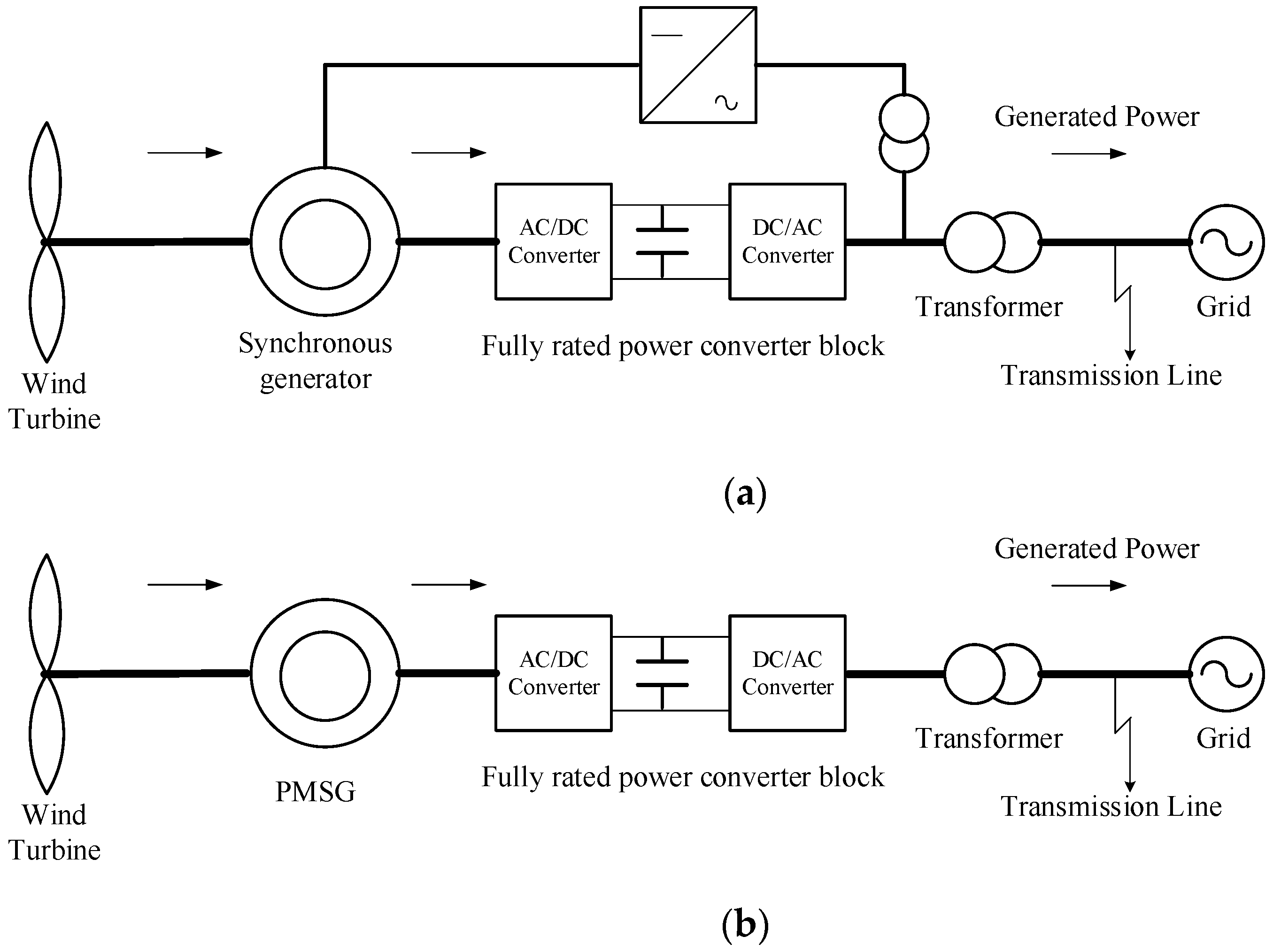
Figure 1. (a) Wind turbine system with full-power converter generator (synchronous generator); (b) Wind turbine system with full-power converter generator (permanent-magnet synchronous generator).
Actuators 11 00203 g001
Figure 2. Physical model of DFIG-based wind generation system.
Actuators 11 00203 g002
Figure 3. DFIG shaft system, represented by a two-mass model.
Actuators 11 00203 g003
Figure 4. Equivalent circuit of DFIG in synchronous reference frame.
Actuators 11 00203 g004
Figure 5. Two axis reference frames for DFIG.
Actuators 11 00203 g005
Figure 6. Rotor-side converter controller block.
Actuators 11 00203 g006
Figure 7. PLL model.
Actuators 11 00203 g007
Figure 8. Grid-side converter controller.
Actuators 11 00203 g008
Figure 9. Block diagram for PSS with transformation technique.
Actuators 11 00203 g009
Figure 10. RSC with transformation PSS.
Actuators 11 00203 g010
Figure 11. QL controller design on RSC.
Actuators 11 00203 g011
Figure 12. QL controller design on GSC.
Actuators 11 00203 g012
Figure 13. Block diagram with QL controller.
Actuators 11 00203 g013
Figure 14. TD3 agent implementation on RSC.
Actuators 11 00203 g014
Figure 15. TD3 agent training progress.
Actuators 11 00203 g015
Figure 16. (a) Active power and (b) reactive power with and without PSS.
Actuators 11 00203 g016
Figure 17. (a) DC-link voltage and (b) generator speed with PSS.
Actuators 11 00203 g017
Figure 18. (a) Active power and (b) reactive power with and without PSS during three-phase fault condition.
Actuators 11 00203 g018
Figure 19. (a) Active power and (b) reactive power with and without PSS during single-phase short circuit fault condition.
Actuators 11 00203 g019
Figure 20. Active power response at 18th iteration.
Actuators 11 00203 g020
Figure 21. Active power response at 25th iteration.
Actuators 11 00203 g021
Figure 22. Reactive power with QL.
Actuators 11 00203 g022
Figure 23. (a) Wind speed change and (b) generator speed per unit.
Actuators 11 00203 g023
Figure 24. Active power with PI controller vs. Q-learning.
Actuators 11 00203 g024
Figure 25. Reactive power with PI controller vs. Q-learning.
Actuators 11 00203 g025
Figure 26. Active power with PI controller vs. Q-learning under fault.
Actuators 11 00203 g026
Figure 27. Reactive power with PI controller vs. Q-learning under fault.
Actuators 11 00203 g027
Figure 28. Wind speed variation in Ottawa region.
Actuators 11 00203 g028
Figure 29. Average wind speed variation in Ottawa region.
Actuators 11 00203 g029
Figure 30. Active power with TD3 agent vs. Q-learning.
Actuators 11 00203 g030
Figure 31. Reactive power with TD3 agent vs. Q-learning.
Actuators 11 00203 g031
Figure 32. DC-link voltage with TD3 agent vs. Q-learning.
Actuators 11 00203 g032
Figure 33. Generator speed with TD3 agent vs. Q-learning.
Actuators 11 00203 g033
Table 1. Small-signal model eigenvalues and state variables.
λ = σ ± j ω State Variables Δ X
λ 4 , λ 5 5.02 ± 389.67 i i d r   and   i q r
λ 6 , λ 7 73.54 ± 376.36 i i q s   and   x 7
λ 8 , λ 9 64 ± 37.08 i V d c   and   x 5
λ 12 , λ 13 10.34 ± 8.47 i v q s   and   θ p l l
λ 19 , λ 20 0.0019 ± 0.93 i x 2 ,   x 4
λ 11 , λ 21 16.16 ± 1.79 i x 1   and   θ f
Publisher’s Note: MDPI stays neutral with regard to jurisdictional claims in published maps and institutional affiliations.