Output Feedback Tracking Sliding Mode Control for Systems with State- and Input-Dependent Disturbances

Abstract

In this paper, output feedback tracking sliding mode control was considered for uncertain multivariable linear systems. The uncertainties included external disturbance, the system state, and control input. A new property of the loop transfer recovery (LTR) observer was first established: the state estimation error of the LTR observer can be made arbitrarily small with respect to state- and input-dependent system uncertainties. Observer-based output feedback tracking sliding mode control using the LTR observer is presented. The proposed sliding mode control approach can maintain the boundedness of the system state and drive the system outputs arbitrarily close to the desired reference outputs; the degree of closeness was determined by a design parameter in the LTR observer. In the proposed approach, the most general and simple observer-based output feedback control formulation was used to achieve global tracking. Simulations with a two-degree-of-freedom (DOF) robotic manipulator application illustrated the claimed properties, and a peaking and chattering reduction technique was demonstrated to protect the actuator.

1. Introduction

Sliding mode control is a widely recognized and robust control method. For applications in robot manipulators, it has been developed over the past four decades [1,2,3,4,5,6]. In such a design, robustness against parametric uncertainties and unknown disturbances is achieved using a nonlinear switching control law. According to a review of such designs [7,8], early sliding mode control designs mostly operate under the assumption that full state information is available. However, because of technical or economic constraints, this assumption does not hold in actual settings; only output measurement is available in real applications. Therefore, developing output feedback sliding mode control designs is necessary.

Conventionally, the sliding surface is constructed as a static function of the output. To guarantee the existence of the control law, geometric conditions were given in [9] and relaxed in [10]. In [11,12,13], different sliding surfaces structured using a linear matrix inequality technique were used to synthesize the static output feedback control law. An artificial time delay was introduced in the output feedback control law in [14] to relax a stability assumption. Recently, the system structure has been reconsidered using the super-twisted algorithm with variable gain, and the first-order approximation filter has been used to estimate the upper bound for the norm of a partially unmeasured state vector [15]. Most related approaches are hampered by the constraints applied to relative-degree-one systems only.

In output feedback control, a key solution to such problems is the observer-based structure. In this design, the required state information of the control system is estimated by observers or differentiators. For a system with unknown disturbances or uncertainties, constructing a robust observer or differentiator that can provide exact state estimations is the first challenge to be overcome. Related studies aiming to address this matter have reported remarkable results. In [16], a reduced-order observer whose dynamics were decoupled from unknown disturbances was proposed. A sliding mode observer was proposed in [17] for the state estimation of systems subject to unknown disturbances. However, the system must still be a relative-degree-one system. The relative degree constraint was relaxed in [18,19,20] by using high-order sliding mode differentiators or high-gain observers. High-gain observer-based sliding mode control [21,22] can be used for multivariable nonlinear systems with stable zero dynamics, and a higher order sliding mode differentiator can be used to estimate the required output derivatives [23,24,25].

In the observer-based approach, a design branch has focused on combining sliding mode control with the standard model reference adaptive control formulation [26]. With this formulation, the design of output feedback sliding mode control for relative-degree-one systems is straightforward [27,28]. When the system relative degree is larger than one, the design becomes complicated, with too many filters required [29,30]. Some researchers have employed simpler approaches by using small-parameter filtering [31], a high-gain observer [32], a lead filter design [33], or a higher order sliding mode differentiator [34,35] to estimate the time derivatives of the system output. With the output derivatives available, the difficulty of the control problem for a system with a relative degree larger than one is reduced to that for a relative-degree-one system.

In this paper, a novel design was proposed for observer-based output feedback sliding mode control. The proposed design relies on a robust observer, termed the loop transfer recovery (LTR) observer. The LTR observer [36] was originally utilized to recover the robustness properties, such as the phase margin and gain margin, of linear quadratic Gaussian (LQG) control [37]. This paper exploited the novel advantage of having an LTR observer, namely, the state estimation error of the LTR observer can be arbitrarily small with respect to the state- and input-dependent system uncertainties. The resultant LTR observer-based output feedback sliding mode control drives the system state into a small residual set around the origin, with the size of the residual set controlled by a design parameter in the observer Riccati equation.

Most other output feedback sliding mode control designs constrain unknown uncertainties, thus depending on the system output or time [9,11,12,13,14,16,17,18,19,20,21,22,23,24,28,29,30,32,33,34]. However, state-dependent uncertainties are prevalent in mechanical systems [38], electronic circuits [39], and robot manipulators [6]; dealing with such uncertainties has become a pertinent research topic [15,35,38]. First, in this paper, unknown disturbances were further extended to input- and state-dependent disturbances, which are the most widely encountered related research. Such an endeavor is considerably challenging because such uncertainties are potentially unbounded, and the input-dependent uncertainties further complicate analysis when sliding mode control is used. Second, the output feedback sliding mode control method detailed in this paper offered global stability, whereas designs [23,24,25] based on higher order sliding mode differentiators are only locally or semiglobally stable. Third, the proposed sliding mode control design was intuitively and structurally simpler than the variable-structure model reference of adaptive control [27,28,29,30,31,32,33,34,35], high-gain observer sliding mode control [21,22], the super-twisted algorithm [15], and the design based on a higher order sliding mode differentiator [23,24,25]; hence, it can be easily accepted by control engineers with only fundamental control knowledge. In [15,34,35], multiple estimators were employed to guarantee global stability. By contrast, in they present study, only one Luenberger-type observer was used. Fourth, the approach described in this paper required minimum system information. The proposed design did not impose relative-degree-one constraints on the original controlled system structure as in [9,10,11,13,14,15,16,17,20,28,29] or require a priori knowledge of the system’s relative degree and upper bound of disturbance as in [27,28,29,30,31,32,33,34,35]. Furthermore, herein, assumptions on disturbance in [10,13] and the system structure in [10,11,13,14,21,22,23,40] were waived, and the design procedure proposed did not require any state transformation. The most general system structure was considered in this paper; the application of the related approach was therefore straightforward. In the application in a robot manipulator, the proposed design used only joint position and input torque command, whereas the information of system matrices in the dynamic equation [3,4] or the estimation of system matrices [5] were requested in the control design. Moreover, the stability analysis in this paper was independent with the matrices in the governing equation of robot dynamics, while [6] required the derivative of the state-dependent system matrix to prove the controller stability. In this paper, a given vector $x\in R^n$, $\parallel x\parallel$ denotes the usual Euclidean two-norm vector.

2. State Feedback Sliding Mode Control

Consider a linear multiple-input multiple-output (MIMO) system subject to unknown, but matched system uncertainties.

$$\begin{array}{cc}\hfill \dot{x}& =Ax+B(u+e_0),e_0=\Delta \kappa u+{\theta }^{T}x+d,\hfill \\ \hfill y& =Cx,\hfill \end{array}$$

(1)

where $x\in R^n$ is the system state, $u\in R^m$ is the control input, $y\in R^m$ is the system output, $(A,B,C)$ are nominal system matrices with proper dimensions, $d\in R^m$ is an unknown time-varying disturbance satisfying a matching condition [41], $\theta \in R^{n\times m}$ contains parametric uncertainty, and $\Delta \kappa \in R^{m\times m}$ is the uncertainty in the control gain matrix. The uncertainties, which may be arbitrarily time-varying and state- and input-dependent, satisfy the upper bounds:

$$\begin{array}{c}\hfill \parallel d\parallel \le D,\parallel \theta \parallel \le \overline{\theta },\parallel \Delta \kappa \parallel \le \overline{\kappa }<1.\end{array}$$

(2)

This condition on $\Delta \kappa$ is more stringent than the Hurwitz condition in [42], but the control in [42] applies to relative-degree-one systems only. The system matrix A may be stable or unstable; the matrix pair $(A,B)$ was assumed to be controllable; $(A,C)$ was assumed to be observable; the number of inputs was equal to that of the outputs; and the nominal system $(A,B,C)$ was assumed to be minimum phase (all finite zeros are stable). System state x was not accessible for measurement, and the only accessible signals were control input u and system output y. The control objective was to drive system output y to track, in the face of system uncertainty $e_0$, desired bounded reference output $y_m$ as closely as possible.

Remark 1.

In most previous research on output feedback sliding mode control, uncertainty was assumed to be a function of disturbance and output, $e_0=\theta y+d$; by contrast, in the proposed approach, uncertainty was allowed to be a function of state, input, and external disturbance: $e_0=\Delta \kappa u+{\theta }^{T}x+d$. This lumped uncertainty was potentially unbounded; the boundedness was uncertain when the stability of the control system (1) was not conclusively demonstrated.

The first step of control design is to transform the tracking control problem into a stabilizing control problem. This can be achieved by establishing a reference model for the bounded reference output $y_m$ as follows:

$$\begin{array}{cc}\hfill {\dot{x}}_m& =(A-BK)x_m+B{r}_m\hfill \\ \hfill y_m& =C{x}_m,\hfill \end{array}$$

(3)

where the reference state $x_m$ and the control command $r_m$ are all bounded but unavailable and the reference output $y_m$ is available for measurement. The system matrix $A-BK$ is stable for some stabilizing state feedback gain K (see the control law (7) below). The aforementioned reference model was temporarily used for analysis purposes. It can be written as:

$$\begin{array}{cc}\hfill {\dot{x}}_m& =A{x}_m+B{u}_m,u_m=-K{x}_m+r_m\hfill \\ \hfill y_m& =C{x}_m,\hfill \end{array}$$

(4)

where $u_m$ is a bounded signal. Defining the error signals $x_e=x-x_m$, $y_e=y-y_m$ and subtracting (4) from (1) yield:

$$\begin{array}{cc}\hfill {\dot{x}}_e& =A{x}_e+B(u+e),\hfill \\ \hfill y_e& =C{x}_e,\hfill \end{array}$$

(5)

where the uncertainty becomes:

$$\begin{array}{cc}\hfill e& =e_0-u_m=\Delta \kappa u+{\theta }^{T}x+d-u_m\hfill \\ \hfill & =\Delta \kappa u+{\theta }^T{x}_e+d-u_m+{\theta }^T{x}_m,\hfill \end{array}$$

(6)

in which ${\theta }^T{x}_e$ is potentially unbounded prior to obtaining the proof of the stability of the proposed control design, and $-u_m+{\theta }^T{x}_m$ is unknown but bounded. If a stabilizing control design u can be constructed to drive the error state $x_e$ in (5) to zero, the tracking mission is achieved. Thus, the tracking control problem for the system (1) is transformed into a stabilizing control problem for the error system (5).

In this section, a state feedback sliding mode control approach was reviewed for this error system (5) (assuming $x_e$ was accessible for measurement). In the next section, an observer-based output feedback sliding mode control design is presented (assuming only $y_e$ was accessible for measurement). A state feedback sliding mode control design for the error system was constructed as follows.

$$\begin{array}{c}\hfill u=-K{x}_e-\rho \left(x_e\right)\frac{\sigma }{\parallel \sigma \parallel },\end{array}$$

(7)

where $K\in R^{m\times n}$ is the state feedback gain that places the eigenvalues of $A-BK$ in the open left-half plane. As the nominal closed-loop system matrix $A-BK$ is stable, a positive definite matrix $P\in R^{n\times n}$ exists, satisfying the Lyapunov equation (Chapter 5.4 in [43]),

$$\begin{array}{c}\hfill {(A-BK)}^{T}P+P(A-BK)=-(1+\nu )I,\end{array}$$

(8)

where $\nu$ can be any small positive parameter and appears in the equation only for the purpose of conducting a theoretical analysis of closed-loop stability. Without loss of generality, it can be assumed that $\nu =1$. In the control law (7), $\sigma \in R^m$ is the sliding variable:

$$\begin{array}{c}\hfill \sigma =2B^{T}P{x}_e,\end{array}$$

(9)

where P is obtained from the Lyapunov Equation (8) and $\rho \left(x_e\right)\in R$ is a positive, time-varying control gain:

$$\begin{array}{c}\hfill \rho \left(x_e\right)=c_1\parallel x_e\parallel +c_0,c_1\ge \frac{\overline{\theta }}{1-\overline{\kappa }},c_0\ge \frac{\overline{d}}{1-\overline{\kappa }},\end{array}$$

(10)

where $\overline{d}$ is an upper bound of $d-u_m+{\theta }^T{x}_m$. Conducting stability analysis of the aforementioned state feedback sliding mode control approach (7) based on a Lyapunov function $x_e^{T}P{x}_e$ has become standard (details can be found in Chapter 14.2 in [44]). State feedback sliding mode control (7) can asymptotically drive the error state $x_e$ to zero despite system uncertainties. Thus, the tracking mission of the original system was achieved.

Remark 2.

In the reference model of (4), the structure naturally constrains the reference output $y_m$ to be sufficiently smooth, and the signal should have bounded derivatives for at least n-times differentiations. This property can be explicitly addressed if the reference model (4) is constructed in observable canonical form.

3. Robust Loop Transfer Recovery Observer

In the previous section, state feedback tracking sliding mode control was reviewed. In many real-world applications, full state information is unavailable, and the only accessible signal is the system output. It is therefore desirable to devise a sliding mode control approach that relies on output measurement only. First, a robust observer was constructed to obtain an estimate ${\widehat{x}}_e$ of the error state $x_e$ for the error system (5). Subsequently, all of state $x_e$ in the state feedback sliding mode control law (7) was replaced by state estimate ${\widehat{x}}_e$.

The robust observer proposed in this paper was the LTR observer. The original purpose of the LTR observer [36] was to recover the loop transfer function of the output feedback LQG control to that of the state feedback LQ control. Consequently, favorable and robust properties such as a large gain margin and phase margin were achieved against unstructured and unmodeled dynamics. However, related studies on the LTR observer have not revealed the upper bounds of the estimation errors when system uncertainties are present. In this paper, an upper bound of the state estimation error was explicitly derived. On the basis of this upper bound, the LTR observer can be used for robust sliding mode control of uncertain systems.

Consider the system (5) with accessible output $y_e$ but inaccessible state $x_e$. The LTR observer had the usual structure of a Luenberger observer and was constructed as follows:

$$\begin{array}{cc}\hfill {\dot{\widehat{x}}}_e& =A{\widehat{x}}_e+Bu+L(y_e-C{\widehat{x}}_e),L=Q{C}^T/\mu ,\hfill \end{array}$$

(11)

where ${\widehat{x}}_e$ is an estimation of the system state $x_e$ and $Q\in R^{n\times n}$ is the solution matrix of the observer Riccati equation:

$$\begin{array}{c}\hfill Q{(A+\delta I)}^T+(A+\delta I)Q-\frac{Q{C}^{T}CQ}{\mu }+\xi B{B}^T=0,\end{array}$$

(12)

where $\mu >0,\delta >0$, and $\xi >0$ are scalar design parameters. The initial condition of the observer, ${\widehat{x}}_e\left(0\right)$, can be of any finite value and does not affect the estimation error stability. Normally, ${\widehat{x}}_e\left(0\right)=0$ is chosen. In the LTR observer design, $\delta >0$ was used to control the convergent speed of the state estimation error, and a value for $\xi >0$ that was sufficiently large was selected to ensure a small estimation error with respect to system uncertainty e.

The following lemma presents a well-known result in the study of LTR observers. Because the system $(A,B,C)$ was a minimum-phase system, a positive number $\delta$ existed such that $(A+\delta I,B,C)$ was also a minimum phase system.

Lemma 1.

If $(A+\delta I,B,C)$ is the minimum phase, then the solution Q for the Riccati Equation (12) satisfies ${lim}_{\xi \to \infty }Q/\xi =0$.

Proof. 

See [45]. □

On the basis of Lemma 1, the theorem that follows proved that the LTR observer obtained only a small estimation error with respect to system uncertainty e in (5). The theorem enabled the derivation of an explicit upper bound of the state estimation error. According to this upper bound, the larger the design parameter $\xi$ in the observer Riccati Equation (12) is, the smaller the state estimation error is. This theorem was a novel addition to the literature. Previous research on the LTR observer [36,46] has only detailed the loop transfer function recovery property of the LTR observer, without an explicit upper bound of the estimation error.

Theorem 1.

The LTR observer (11) asymptotically (as time approached infinity) achieved a small estimation error ${\tilde{x}}_e=x_e-{\widehat{x}}_e$ for the error system (5) in the sense that:

$$\begin{array}{c}\hfill \parallel {\tilde{x}}_e\left(t\right)\parallel \le ϵ(\overline{\kappa }\parallel u\parallel +\overline{\theta }\parallel x_e\parallel +\overline{d})\end{array}$$

(13)

where:

$$\begin{array}{c}\hfill ϵ=\sqrt{\overline{\sigma }\left(\frac{Q}{\delta \xi }\right)}\to 0\mathrm{as}\xi \to \infty ,\end{array}$$

(14)

in which $\overline{\sigma }(·)$ denotes the maximum singular value.

Proof. 

Define the state estimation error ${\tilde{x}}_e=x_e-{\widehat{x}}_e$. From (5) and (11), the dynamics of ${\tilde{x}}_e$ is given as:

$$\begin{array}{c}\hfill {\dot{\tilde{x}}}_e=(A-LC){\tilde{x}}_e+Be.\end{array}$$

(15)

Choose the Lyapunov function $V={{\tilde{x}}_e}^T{Q}^{-1}{\tilde{x}}_e$, where Q is the solution matrix from the Riccati Equation (12). Checking the time derivative of V along the trajectory of ${\tilde{x}}_e$ gives:

$$\begin{array}{c}\hfill \dot{V}\le -2\delta V-\frac{1}{\mu }\parallel C{\tilde{x}}_e{\parallel }^2-\xi \parallel {\tilde{x}}_e^T{Q}^{-1}{B\parallel }^2+2\parallel {\tilde{x}}_e^T{Q}^{-1}B\parallel ·\parallel e\parallel .\end{array}$$

In the aforementioned equation, the maximum of the last two terms occurs when $\parallel {\tilde{x}}_e^T{Q}^{-1}B\parallel =\parallel e\parallel /\xi$, with the maximum being ${\parallel e\parallel }^2/\xi$. Hence,

$$\begin{array}{cc}\hfill \dot{V}& \le -2\delta V-\frac{1}{\mu }{\parallel C{\tilde{x}}_e\parallel }^2+\frac{{\parallel e\parallel }^2}{\xi }\hfill \\ \hfill & \le -2\delta V+\frac{{\parallel e\parallel }^2}{\xi }\hfill \\ \hfill & =-\delta V-\delta (V-\frac{{\parallel e\parallel }^2}{\delta \xi }).\hfill \end{array}$$

(16)

The last inequality shows that V decreases exponentially as long as $V\ge {\parallel e\parallel }^2/\left(\delta \xi \right)$; thus, it can be concluded that $V\left(t\right)\le {\parallel e\parallel }^2/\left(\delta \xi \right)$ as time approaches infinity. The use of $V\ge \underline{\sigma }\left(Q^{-1}\right)\parallel {\tilde{x}}_e{\parallel }^2={\parallel {\tilde{x}}_e\parallel }^2/\overline{\sigma }\left(Q\right)$ produces:

$$\begin{array}{cc}\hfill \parallel {\tilde{x}}_e\left(t\right)\parallel & \le \sqrt{\overline{\sigma }\left(\frac{Q}{\delta \xi }\right)}\parallel e\left(t\right)\parallel \hfill \\ \hfill & =ϵ\parallel \Delta \kappa u+{\theta }^T{x}_e+d-u_m+{\theta }^T{x}_m\parallel \hfill \\ \hfill & \le ϵ(\overline{\kappa }\parallel u\parallel +\overline{\theta }\parallel x_e\parallel +\overline{d})\hfill \end{array}$$

(17)

where:

$$\begin{array}{c}\hfill ϵ=\sqrt{\overline{\sigma }\left(\frac{Q}{\delta \xi }\right)},\mathrm{as}t\to \infty ,\end{array}$$

(18)

and the last inequality is obtained by substitution of the definition of $\overline{d}$ (10).

In the definition provided for $ϵ$, $\delta$ was fixed in the design. Hence, according to Lemma 1, $ϵ$ became arbitrarily small as the selected design parameter $\xi$ became sufficiently large. This proves the theorem. □

Remark 3.

In Theorem 1, the estimation error ${\tilde{x}}_e$ was bounded by the control signal $\parallel u\parallel$ and system state vector $\parallel x_e\parallel$; therefore, it can only be temporarily concluded that the estimation error can be potentially unbounded in this stage. Components u and $x_e$ have the potential to be unbounded because no conclusion on boundedness was made, and the convergency of the state estimation should be examined after stability analysis for the controlled system (5) has been completed.

Remark 4.

Previously, many researchers used a high-gain observer (see Chapter 14.5 of [44]) to estimate the system state in their sliding mode control design. However, the high-gain observer is subject to the constraint that the system must have no zero dynamics; that is, the system relative degree is equal to the system dimension. As a result, when the high-gain observer is applied to the sliding mode control design for systems with an arbitrary relative degree [21,22,32], the high-gain observer can estimate only the partial state (the external state) of the system, while the LTR observer in this paper can estimate the full state of the system, providing more monitoring information of the system.

Remark 5.

In (11), the design of the robust observer has the usual structure of the Luenberger observer, which is an intuitive and simple design of a linear state observer. By contrast, for example, the higher order sliding mode differentiator follows the nonlinear recursive algorithm [23]:

$$\begin{array}{cc}\hfill {\dot{z}}_0& =v_0,\hfill \\ \hfill v_0& =-{\lambda }_0{|z_0-y_e\left(t\right)|}^{n/(n+1)}sign(z_0-y_e\left(t\right))+z_1\hfill \\ \hfill {\dot{z}}_1& =v_1,\hfill \\ \hfill v_1& =-{\lambda }_1{|z_1-v_0|}^{(n-1)/\left(n\right)}sign(z_1-v_0)+z_2\hfill \\ \hfill ⋮& \\ \hfill {\dot{z}}_{n-1}& =v_{n-1},\hfill \\ \hfill v_{n-1}& =-{\lambda }_{n-1}{|z_{n-1}-v_{n-2}|}^{1/2}sign(z_{n-1}-v_{n-2})+z_n\hfill \\ \hfill {\dot{z}}_n& =-{\lambda }_{n}sign(z_n-v_{n-1}),\hfill \end{array}$$

(19)

where $z_i$ is an estimation of the ith-order derivative of $y_e\left(t\right)$, and ${\lambda }_i(i,L)$ is a function of i and L, in which L stands for the known Lipschitz constant of the nth derivative of $y_e\left(t\right)$. Comparing (11) and (19), it is seen that a higher order sliding mode differentiator (19) has a more complex structure and requires more computation effort to estimate the desired system information.

4. Output Feedback Sliding Mode Control

As detailed in the previous section, a state estimate ${\widehat{x}}_e$ was obtained from the LTR observer (11). Next, the observer-based output feedback tracking sliding mode control can be established by replacing $x_e$ in the state feedback control law (7) with its estimate ${\widehat{x}}_e$. The resultant output feedback sliding mode control equation is as follows:

$$\begin{array}{c}\hfill u=-K{\widehat{x}}_e-\rho \left({\widehat{x}}_e\right)\frac{\widehat{\sigma }}{\parallel \widehat{\sigma }\parallel },\end{array}$$

(20)

where the estimated sliding variable is:

$$\begin{array}{c}\hfill \widehat{\sigma }=2B^{T}P{\widehat{x}}_e,\end{array}$$

(21)

and the switching control gain is chosen as:

$$\begin{array}{c}\hfill \rho \left({\widehat{x}}_e\right)=c_1\parallel {\widehat{x}}_e\parallel +c_0,\end{array}$$

(22)

with:

$$\begin{array}{c}\hfill c_1\ge \frac{\overline{\kappa }\parallel K\parallel +\overline{\theta }}{\beta \gamma -\overline{\kappa }},c_0\ge \frac{\overline{d}}{\beta \gamma -\overline{\kappa }},\end{array}$$

(23)

in which $\beta$ and $\gamma$ are two positive constants to be defined. The choice of constants $c_0$ and $c_1$ in (22) is different from that in (10).

Given the uncertainty upper bounds $\overline{\kappa }\in [0,1)$, $\overline{\theta }$, the norm of state feedback gain $\parallel K\parallel$, and a sufficiently small $ϵ$ in Theorem 1, a constant $\beta \in (\overline{\kappa },1)$ exists such that:

$$\begin{array}{c}\hfill \beta ·\gamma >\overline{\kappa },\mathrm{where}\gamma =\frac{1-ϵ\overline{\theta }}{1+ϵ\parallel K\parallel }.\end{array}$$

(24)

The aforementioned inequality ensures that the denominator in (23) is positive. Given $\beta$ as chosen, define another constant $\alpha$:

$$\begin{array}{c}\hfill \alpha =\frac{1-\beta }{1+\beta },\mathrm{with}\alpha \in (0,1).\end{array}$$

(25)

The virtual constants $\alpha$ and $\beta$ were used only in the following closed-loop stability analysis for the MIMO system (1). The stability analysis was nontrivial for the MIMO system. In the case that the system is a single-input single-output system, the stability analysis can be considerably simplified, without the need to define the constants $\alpha$ and $\beta$.

To simplify the equation derivations in the stability analysis, the following lemma should be constructed in advance.

Lemma 2.

The following inequalities hold for the system (1) and sliding mode control (20).

(i) 

$\parallel {\tilde{x}}_e\parallel \le ϵ\left[\right(\overline{\kappa }\parallel K\parallel +\overline{\theta })\parallel {\widehat{x}}_e\parallel +\overline{\kappa }\rho \left({\widehat{x}}_e\right)+\overline{d}]/(1-ϵ\overline{\theta })$.

(ii) 

$\parallel K{\tilde{x}}_e+e\parallel \le \beta \rho \left({\widehat{x}}_e\right)$.

(iii) 

$\parallel {\tilde{x}}_e\parallel \le ϵ(f_1\parallel x_e\parallel +f_0)$ for some positive constants $f_1$ and $f_0$.

(iv) 

$\parallel \rho \left({\widehat{x}}_e\right)\parallel \le g_1\parallel x_e\parallel +g_0$ for some positive constants $g_1$ and $g_0$,

where ϵ is as in (14).

Proof. 

(i) The control law (20) suggests that:

$$\begin{array}{c}\hfill \parallel u\parallel \le \parallel K\parallel ·\parallel {\widehat{x}}_e\parallel +\rho \left({\widehat{x}}_e\right)\le (\parallel K\parallel +c_1)\parallel {\widehat{x}}_e\parallel +c_0.\end{array}$$

(26)

One continues to derive:

$$\begin{array}{cc}\hfill \parallel {\tilde{x}}_e\parallel & \le ϵ\overline{\kappa }\parallel u\parallel +ϵ\overline{\theta }\parallel x_e\parallel +ϵ\overline{d}\hfill \\ \hfill & \le ϵ\overline{\kappa }(\parallel K\parallel +c_1)\parallel {\widehat{x}}_e\parallel +ϵ\overline{\theta }\parallel x_e\parallel +ϵ(\overline{\kappa }{c}_0+\overline{d})\hfill \\ \hfill & \le ϵ(\overline{\kappa }\parallel K\parallel +\overline{\theta })\parallel {\widehat{x}}_e\parallel +ϵ\overline{\theta }\parallel {\tilde{x}}_e\parallel +ϵ\overline{\kappa }\rho \left({\widehat{x}}_e\right)+ϵ\overline{d}\hfill \\ \hfill & \le \frac{ϵ}{1-ϵ\overline{\theta }}\left[\right(\overline{\kappa }\parallel K\parallel +\overline{\theta })\parallel {\widehat{x}}_e\parallel +\overline{\kappa }\rho \left({\widehat{x}}_e\right)+\overline{d}],\hfill \end{array}$$

(27)

where the first inequality follows from Theorem 1, the second follows from (26), the third follows from the inequality $\parallel x_e\parallel \le \parallel {\widehat{x}}_e\parallel +\parallel {\tilde{x}}_e\parallel$ and (22), and the last is obtained by rearranging the equation;

(ii)

With the upper bound in (i), an upper bound for $K{\tilde{x}}_e+e$ can be derived,

$$\begin{array}{cc}\hfill \parallel K{\tilde{x}}_e& +e\parallel \le \parallel K\parallel \parallel {\tilde{x}}_e\parallel +\parallel e\parallel \hfill \\ \hfill & \le ϵ\parallel K\parallel (\overline{\kappa }\parallel u\parallel +\overline{\theta }\parallel x_e\parallel +\overline{d})+(\overline{\kappa }\parallel u\parallel +\overline{\theta }\parallel x_e\parallel +\overline{d})\hfill \\ \hfill & =(1+ϵ\parallel K\parallel )(\overline{\kappa }\parallel u\parallel +\overline{\theta }\parallel x_e\parallel +\overline{d})\hfill \\ \hfill & \le (1+ϵ\parallel K\parallel )[\overline{\kappa }(\parallel K\parallel +c_1)\parallel {\widehat{x}}_e\parallel +\overline{\theta }\parallel x_e\parallel +(\overline{\kappa }{c}_0+\overline{d})]\hfill \\ \hfill & \le (1+ϵ\parallel K\parallel )\left[\right(\overline{\kappa }\parallel K\parallel +\overline{\theta })\parallel {\widehat{x}}_e\parallel +\overline{\theta }\parallel {\tilde{x}}_e\parallel +\overline{\kappa }\rho \left({\widehat{x}}_e\right)+\overline{d}]\hfill \\ \hfill & \le \frac{1+ϵ\parallel K\parallel }{1-ϵ\overline{\theta }}\left[\right(\overline{\theta }+\overline{\kappa }\parallel K\parallel )\parallel {\widehat{x}}_e\parallel +\overline{\kappa }\rho \left({\widehat{x}}_e\right)+\overline{d}]\hfill \\ \hfill & \le \frac{1}{\gamma }\left[\right(\overline{\theta }+\overline{\kappa }\parallel K\parallel )\parallel {\widehat{x}}_e\parallel +\overline{\kappa }\rho \left({\widehat{x}}_e\right)+\overline{d}]\le \beta \rho \left({\widehat{x}}_e\right),\hfill \end{array}$$

where the second inequality results from (5) and (13), the third inequality follows from (26), the fourth inequality follows from the inequality $\parallel x_e\parallel \le \parallel {\widehat{x}}_e\parallel +\parallel {\tilde{x}}_e\parallel$ and (22), the fifth inequality results from Part (i) of the lemma, and $\gamma$ is as defined in (24). The last inequality is derived using the inequalities in (22) and (24);

(iii)

In this section, an alternative upper bound is presented for the estimation error ${\tilde{x}}_e$:

$$\begin{array}{cc}\hfill \parallel {\tilde{x}}_e\parallel & \le ϵ\overline{\kappa }\parallel u\parallel +ϵ\overline{\theta }\parallel x_e\parallel +ϵ\overline{d}\hfill \\ \hfill & \le ϵ\overline{\kappa }(\parallel K\parallel +c_1)\parallel {\widehat{x}}_e\parallel +ϵ\overline{\theta }\parallel x_e\parallel +ϵ(\overline{\kappa }{c}_0+\overline{d})\hfill \\ \hfill & \le ϵ\overline{\kappa }(\parallel K\parallel +c_1)\parallel {\tilde{x}}_e\parallel +(ϵ\overline{\theta }+ϵ\overline{\kappa }(\parallel K\parallel +c_1\left)\right)\parallel x_e\parallel +ϵ(\overline{\kappa }{c}_0+\overline{d})\hfill \\ \hfill & \le ϵ(f_1\parallel x_e\parallel +f_0),\hfill \end{array}$$

with

$$\begin{array}{c}\hfill f_1=\frac{\overline{\theta }+\overline{\kappa }\parallel K\parallel +\overline{\kappa }{c}_1}{1-ϵ(\overline{\kappa }\parallel K\parallel +\overline{\kappa }{c}_1)},f_0=\frac{\overline{\kappa }{c}_0+\overline{d}}{1-ϵ(\overline{\kappa }\parallel K\parallel +\overline{\kappa }{c}_1)}.\end{array}$$

(28)

In the aforementioned equations, the first inequality follows from Theorem 1, the second follows from (26), the third follows from the inequality $\parallel {\widehat{x}}_e\parallel \le \parallel x_e\parallel +\parallel {\tilde{x}}_e\parallel$, and the last is obtained by rearranging the equation;

(iv)

According to (22),

$$\begin{array}{cc}\hfill \rho \left({\widehat{x}}_e\right)& =c_1\parallel {\widehat{x}}_e\parallel +c_0\hfill \\ \hfill & \le c_1\parallel x_e\parallel +c_1\parallel {\tilde{x}}_e\parallel +c_0\hfill \\ \hfill & \le (c_1+ϵc_1{f}_1)\parallel x_e\parallel +c_0+ϵc_1{f}_0,\hfill \end{array}$$

where the second inequality is derived from $\parallel {\widehat{x}}_e\parallel \le \parallel x_e\parallel +\parallel {\tilde{x}}_e\parallel$ and the last inequality is obtained from Part (iii) of the lemma. Thus, Part (iv) is proven with $g_1=c_1+ϵc_1{f}_1$ and $g_0=c_0+ϵc_1{f}_0$. □

Before closed-loop stability was proven, the system uncertainty $e=\Delta \kappa u+{\theta }^{T}x+d-u_m+{\theta }^T{x}_m$ in (13) was potentially unbounded. Hence, the state estimation error $\parallel {\tilde{x}}_e\parallel$ in (13) was also potentially unbounded. Determining whether the proposed observer-based state feedback tracking sliding mode control (20) was stabilizing required a rigorous stability analysis. This was accomplished using the main theorem that follows.

Theorem 2.

The LTR observer-based output feedback tracking sliding mode control (20) stabilized an uncertain system (1) in that the system state $x_e$ was driven into an arbitrarily small residue set around the origin if the design parameter ξ in the observer Riccati Equation (12) was sufficiently large.

Proof. 

Choose a Lyapunov function candidate $W=x_e^{T}P{x}_e$ for the controlled error system (5), where the matrix P is from the Lyapunov Equation (8). Taking the time derivative of W along the trajectory of the error system (5) controlled by the output feedback sliding mode control (20) yields:

$$\begin{array}{cc}\hfill \dot{W}& =x_e^T[{(A-BK)}^{T}P+P(A-BK)]x_e+{\sigma }^T[-\rho \left({\widehat{x}}_e\right)\frac{\widehat{\sigma }}{\parallel \widehat{\sigma }\parallel }+K{\tilde{x}}_e+e]\hfill \\ \hfill & =-(1+\nu )\parallel x_e{\parallel }^2-\rho \left({\widehat{x}}_e\right)\frac{{\sigma }^T\widehat{\sigma }}{\parallel \widehat{\sigma }\parallel }+{\sigma }^T[K{\tilde{x}}_e+e],\hfill \end{array}$$

(29)

where e is the lumped system uncertainty $e=\Delta \kappa u+{\theta }^T{x}_e+d-u_m+{\theta }^T{x}_m$. With $\tilde{\sigma }=\sigma -\widehat{\sigma }$, two possible cases may exist in the above equation.

Case 1 (reaching mode): $\parallel \tilde{\sigma }\parallel <\alpha \parallel \sigma \parallel$, where $\alpha \in (0,1)$ is from (25). In this case, using the two inequalities $\parallel \widehat{\sigma }\parallel =\parallel \sigma -\tilde{\sigma }\parallel \le \parallel \sigma \parallel +\parallel \tilde{\sigma }\parallel <(1+\alpha )\parallel \sigma \parallel$ and ${\sigma }^T\tilde{\sigma }\le \parallel \sigma \parallel ·\parallel \tilde{\sigma }{\parallel <\alpha \parallel \sigma \parallel }^2$ can produce:

$$\begin{array}{c}\hfill -\frac{{\sigma }^T\widehat{\sigma }}{\parallel \widehat{\sigma }\parallel }=-\frac{{\sigma }^T\sigma -{\sigma }^T\tilde{\sigma }}{\parallel \sigma -\tilde{\sigma }\parallel }<-\frac{{\parallel \sigma \parallel }^2-\alpha {\parallel \sigma \parallel }^2}{\parallel \sigma \parallel +\alpha \parallel \sigma \parallel }=-\frac{1-\alpha }{1+\alpha }\parallel \sigma \parallel ,\end{array}$$

where $-\frac{1-\alpha }{1+\alpha }\parallel \sigma \parallel =-\beta \parallel \sigma \parallel$ from (25). The inequality (29) then becomes:

$$\begin{array}{cc}\hfill \dot{W}& <-(1+\nu )\parallel x_e{\parallel }^2-\rho \left({\widehat{x}}_e\right)\beta \parallel \sigma \parallel +\parallel K{\tilde{x}}_e+e\parallel ·\parallel \sigma \parallel \hfill \\ \hfill & \le -(1+\nu )\parallel x_e{\parallel }^2,\hfill \end{array}$$

(30)

where the second inequality is obtained from Part (ii) of Lemma 2. It can be concluded that in this case, the Lyapunov function W in (30) is strictly decreasing. Moreover, the sliding variable $\sigma$ fulfills the relation:

$$\begin{array}{c}\hfill {\parallel \sigma \parallel }^2={\sigma }^T\sigma =|4x_e^{T}PB{B}^{T}P{x}_e|\le 4\overline{\delta }·{\parallel x_e\parallel }^2\le \frac{4\overline{\delta }}{\underline{\sigma }\left(P\right)}V,\end{array}$$

(31)

where $\overline{\delta }$ is the maximum singular value of the square matrix $PB{B}^{T}P$ and $\underline{\sigma }\left(P\right)$ is the minimum singular value of matrix P. Combining (30) and (31) revealed that the absolute value of the sliding variable $\left|\sigma \right|$ was exponentially decreasing; in this case, the reaching law can be concluded as:

$$\begin{array}{c}\hfill \sigma \to \tilde{\sigma }.\end{array}$$

The statement implies that the sliding variable $\sigma$ reaches $\tilde{\sigma }$, the boundary layer of the sliding surface $\sigma =0$.

Case 2 (sliding mode): $\parallel \tilde{\sigma }\parallel \ge \alpha \parallel \sigma \parallel$. In this case, the system state was restricted in the boundary layer of the sliding surface, and the following can be derived from (29):

$$\begin{array}{cc}\hfill \dot{W}& \le -(1+\nu )\parallel x_e{\parallel }^2+(1+\beta )\rho \left({\widehat{x}}_e\right)\parallel \sigma \parallel \hfill \\ \hfill & <-\frac{1+\nu }{\overline{\lambda }}W+\frac{(1+\beta )}{\alpha }\rho \left({\widehat{x}}_e\right)\parallel \tilde{\sigma }\parallel \hfill \\ \hfill & =-\frac{\nu }{\overline{\lambda }}W-\frac{1}{\overline{\lambda }}[W-\frac{(1+\beta )\overline{\lambda }}{\alpha }\rho \left({\widehat{x}}_e\right)\parallel \tilde{\sigma }\parallel ],\hfill \end{array}$$

(32)

where the first inequality results from Part (ii) of Lemma 2; the second inequality results from the hypothesis of this case; and $\parallel W\parallel \le \overline{\lambda }{\parallel x_e\parallel }^2$, with $\overline{\lambda }$ being the maximum eigenvalue of matrix P. Equation (32) shows that if $W\ge \frac{(1+\beta )\overline{\lambda }}{\alpha }\rho \left({\widehat{x}}_e\right)\parallel \tilde{\sigma }\parallel$, then W decays exponentially. Hence, the following is eventually obtained:

$$\begin{array}{c}\hfill \underset{t\to \infty }{lim}W<\frac{(1+\beta )\overline{\lambda }}{\alpha }\rho \left({\widehat{x}}_e\right)\parallel \tilde{\sigma }\parallel .\end{array}$$

It follows from the definitions of sliding variables in (9) and (21) that $\parallel \tilde{\sigma }\parallel \le \parallel 2B^{T}P\parallel \parallel {\tilde{x}}_e\parallel$. With the inequality $\parallel W\parallel \ge \underline{\lambda }{\parallel x_e\parallel }^2$, where $\underline{\lambda }$ is the minimum eigenvalue of P, the above equation can be written as:

$$\begin{array}{cc}\hfill \parallel x_e{\parallel }^2& <\frac{(1+\beta )\overline{\lambda }}{\alpha \underline{\lambda }}\parallel 2B^{T}P\parallel ·\rho \left({\widehat{x}}_e\right)·\parallel {\tilde{x}}_e\parallel \hfill \\ \hfill & ={\eta }^2·\rho \left({\widehat{x}}_e\right)·\parallel {\tilde{x}}_e\parallel \hfill \\ \hfill & \le ϵ{\eta }^2(f_1\parallel x_e\parallel +f_0\left)\right(g_1\parallel x_e\parallel +g_0),\hfill \\ \hfill & \le ϵ{\eta }^2(h_1\parallel x_e{\parallel +h_0)}^2\mathrm{as}t\to \infty \hfill \end{array}$$

where:

$$\begin{array}{c}\hfill {\eta }^2=\frac{(1+\beta )\overline{\lambda }}{\alpha \underline{\lambda }}\parallel 2B^{T}P\parallel ;\end{array}$$

the second inequality results from Parts (iii) and (iv) of Lemma 2, and in the last inequality, $h_1=max(f_1,g_1)$ and $h_0=max(f_0,g_0)$. Taking the square root of both sides of the last inequality yields:

$$\begin{array}{c}\hfill \parallel x_e\parallel <\sqrt{ϵ}\eta (h_1\parallel x_e\parallel +h_0)<\frac{\sqrt{ϵ}\eta h_0}{1-\sqrt{ϵ}\eta h_1},\mathrm{as}t\to \infty \end{array}$$

(33)

where the second inequality is obtained by rearranging the first inequality. Because according to Theorem 1, ${lim}_{\xi \to \infty }\sqrt{ϵ}=0$, this ensured that the denominator in the above equation was always positive if the design parameter $\xi$ in the LTR observer was sufficiently large. Because $\sqrt{ϵ}$ also appears in the numerator, Equation (33) proves that, eventually, the error dynamic $x_e=x-x_m$ converges to a small residual set around the origin, with the size of the residual set controlled by the design parameter $\xi$ in the LTR observer design; thus, $x\to x_m$ and $y\to y_m$ are arbitrarily close. Furthermore, the result of (33) guaranteed that the estimation error ${\tilde{x}}_e$ in Theorem 1 was made arbitrarily small using Part (iii) of Lemma 2, and the state estimation ${\widehat{x}}_e$ was bounded and made arbitrarily small by the relation $\parallel {\widehat{x}}_e\parallel \le \parallel x_e\parallel +\parallel {\tilde{x}}_e\parallel$. Finally, the control signal u in (20) remained uniformly bounded because all components in it were bounded. □

The following section illustrates the effectiveness of the proposed output feedback sliding mode control scheme (20).

5. Application Example

A two-degree-of-freedom robotic manipulator studied in [4] was used here to illustrate the efficiency of the proposed control design. The dynamic equation of the two-link robot is defined as:

$$\begin{array}{c}\hfill M\left(q\right)\ddot{q}+C(q,\dot{q})\dot{q}+G\left(q\right)+F\dot{q}=\tau ,\end{array}$$

(34)

where $q={[q_1,q_2]}^T$ is the joint position and $\dot{q}$ and $\ddot{q}\in R^2$ are velocity and acceleration vectors; $M\left(q\right)$, $C(q,\dot{q})$, $G\left(q\right)$, and F are the inertia matrix, Coriolis matrix, gravity matrix, and frictional matrix with proper dimensions; $\tau \in R^2$ is the input torque vector. On the basis of the state-space realization proposed in [4], system matrices in the error dynamic (5) are given as:

$$\begin{array}{c}\hfill A=\left[\begin{array}{cccc}0& 1& 0& 0\\ 0& 0& 0& 0\\ 0& 0& 0& 1\\ 0& 0& 0& 0\end{array}\right],B=\left[\begin{array}{cc}0& 0\\ 1& 0\\ 0& 0\\ 0& 1\end{array}\right],C={\left[\begin{array}{cc}1& 0\\ 0& 0\\ 0& 1\\ 0& 0\end{array}\right]}^T\end{array}$$

with $y={[y_1,y_2]}^T={[q_1,q_2]}^T$, and the desired reference trajectory was assigned as $y_m={[y_{m_1},y_{m_2}]}^T={[2sin\left(t\right),sin\left(t\right)]}^T$. In the output feedback tracking sliding mode control algorithm, the design parameters in the observer Riccati Equation (12) were $\mu =1$, $\delta =10$, and $\xi ={10}^{16}$. According to (18) and (33), $\xi$ should be sufficiently large to guarantee estimating and tracking performance. The control law (20) was constructed with a state feedback gain:

$$\begin{array}{c}\hfill K=\left[\begin{array}{cccc}1& 2& 0& 0\\ 0& 0& 1& 2\end{array}\right],\end{array}$$

and positive constants were assigned as $\nu =1$ in (8) and $c_1=c_0=1000$ in (22) to achieve the desired convergent speed of (30) and to satisfy (23). Herein, the torque command was given as $\tau =u$ in (20) without the knowledge of the system matrices $M\left(q\right)$, $C(q,\dot{q})$, $G\left(q\right)$, and F in (34), and the unknown parameters were considered as the state- and input-dependent disturbances in the error dynamic (5). 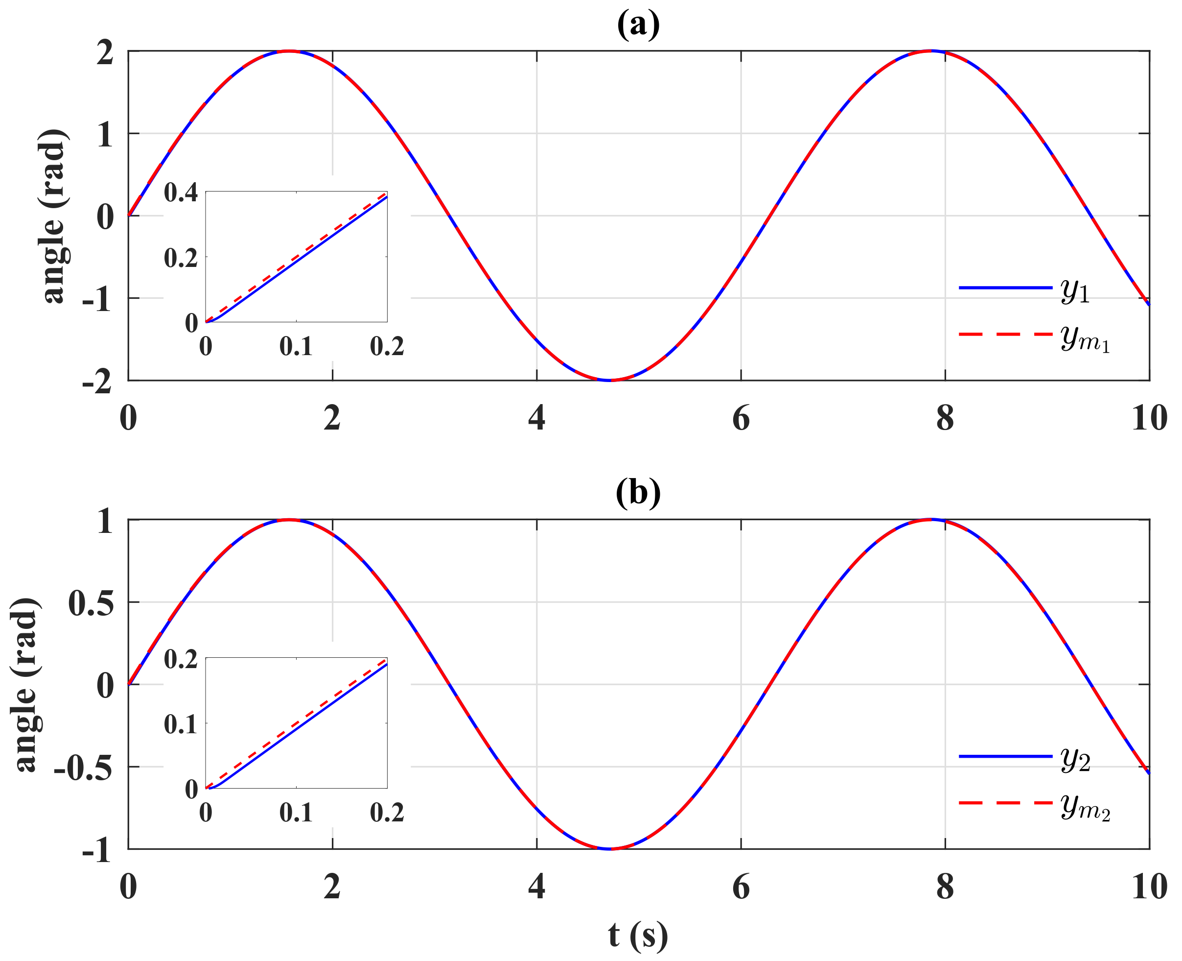Figure 1 shows the tracking performance of the controlled system. Because the initial condition of state estimation ${\widehat{x}}_e$ was set as zero, coinciding with the system error $x_e$, the control system reached the residue set (33) from the very beginning of the simulation. 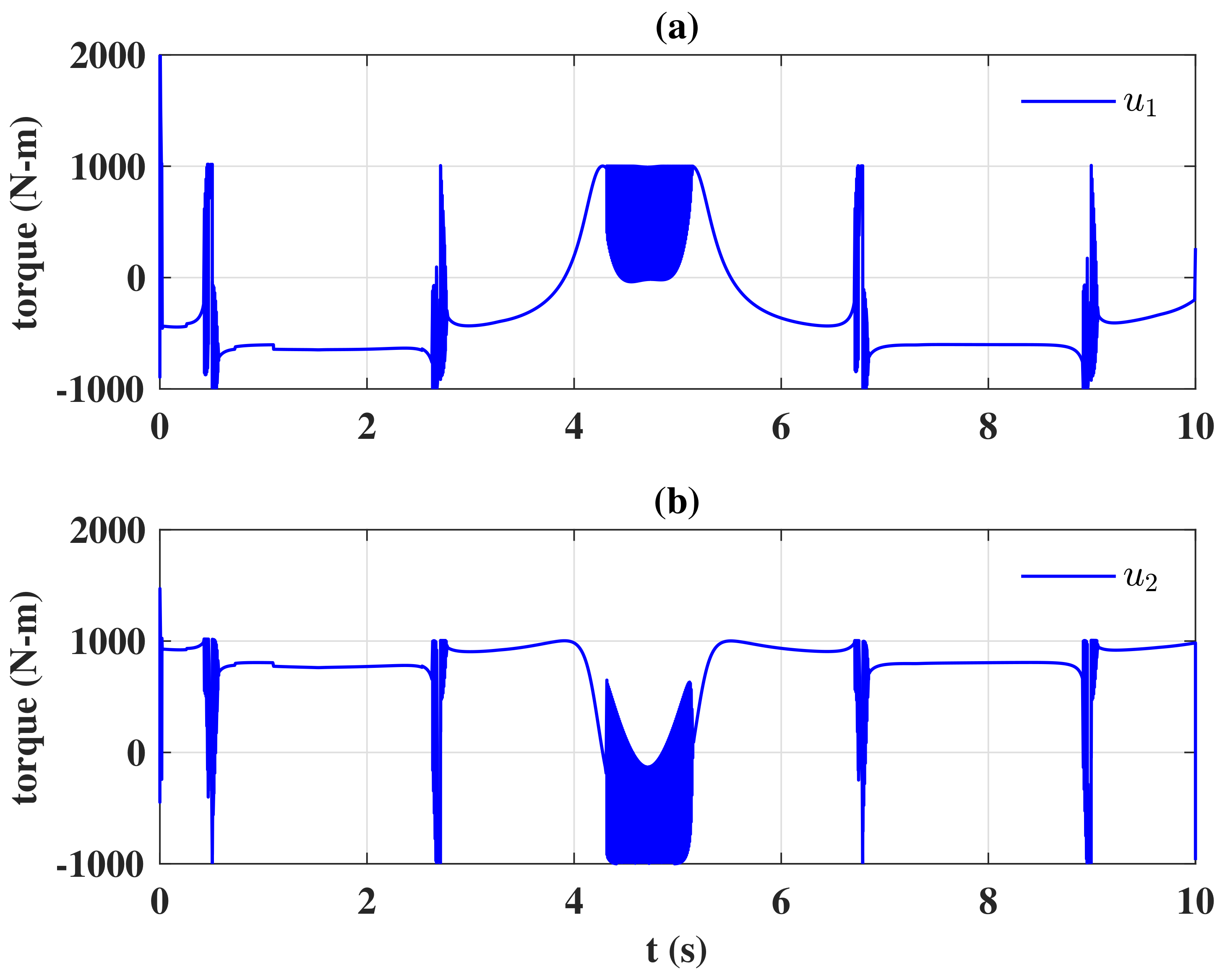Moreover, the parameters $\xi$ in (12) and $\rho$ in (22) were properly chosen; therefore, the system state was constrained in a sufficiently small residue set of error (33), and the two outputs precisely tracked their references; in Figure 1, it is seen the tracking error was a constant from the very initial time. 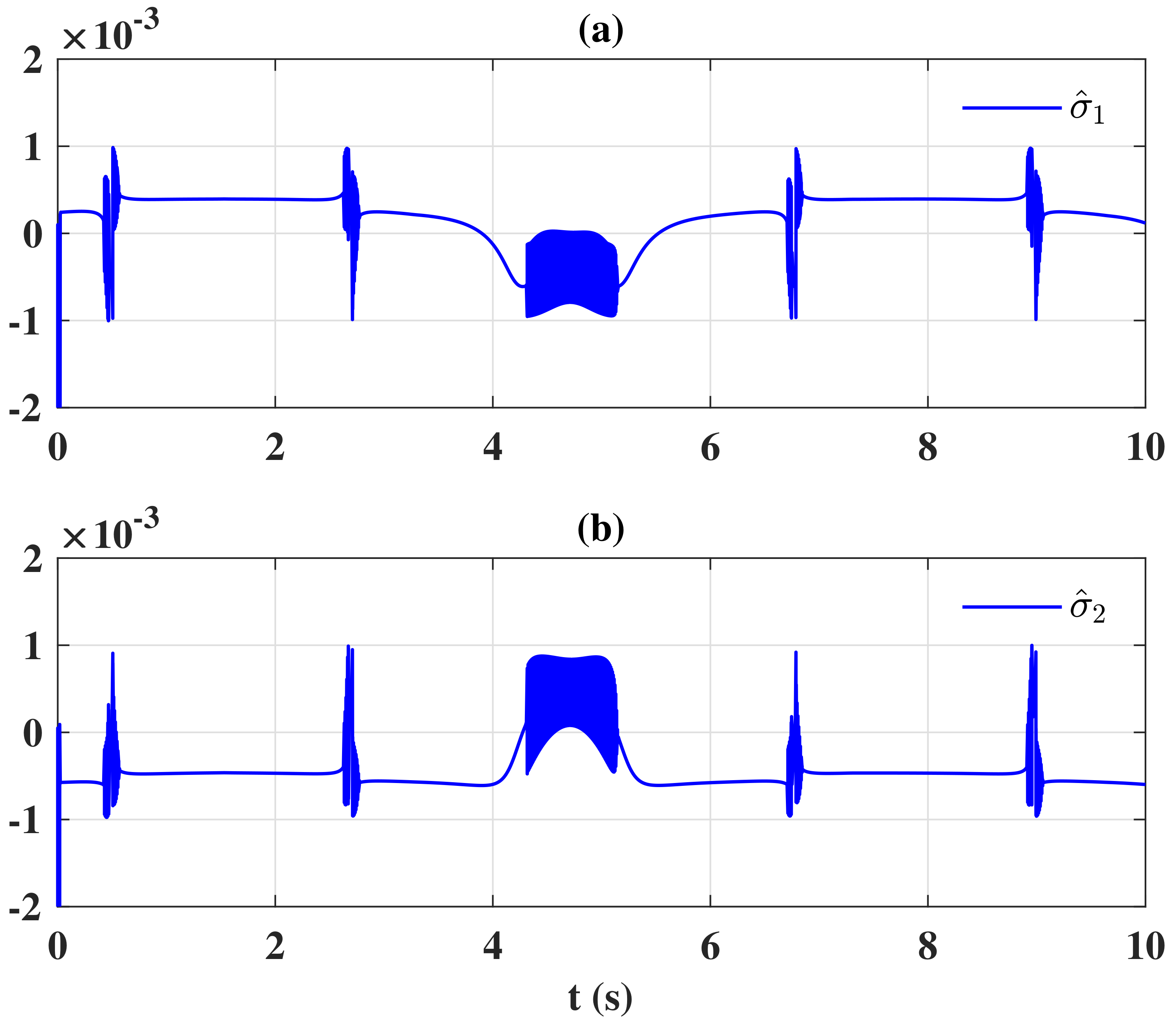The control signals are shown in Figure 2, and Figure 3 presents the sliding variable. It was seen that the control input u rapidly peaked in the very initial time interval; the actuators might be saturated when the control design was implemented. Moreover, because a nonlinear switching function was used in the control law, both control signals were subject to a high-frequency oscillation when the sliding variable $\widehat{\sigma }$ in Figure 3 chattered around $\widehat{\sigma }=0$, which is harmful for actuators in the real world.

To avoid the occurrence of the peaking and chattering phenomenon, the control design (20) was modified as:

$$\begin{array}{c}\hfill u=-K{\widehat{x}}_e-\rho \left({\widehat{x}}_e\right)\frac{\widehat{\sigma }}{\parallel \widehat{\sigma }\parallel +0.001},\end{array}$$

(35)

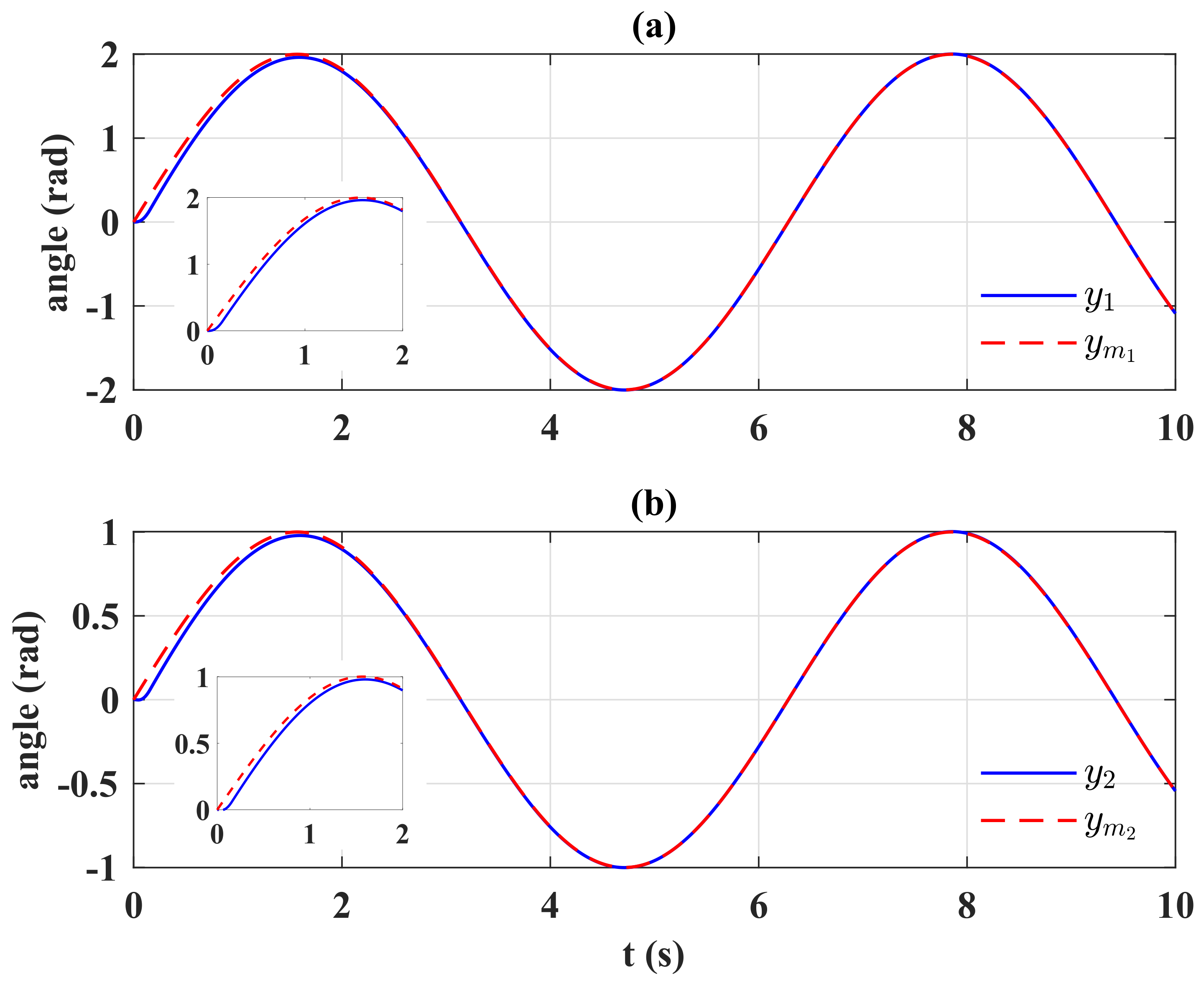
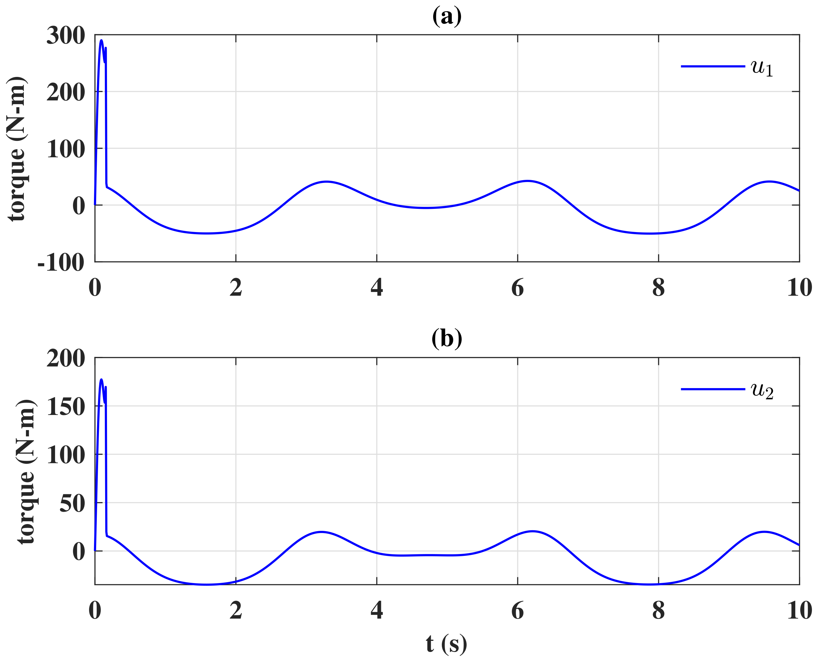
where the discontinuous function $\widehat{\sigma }/\parallel \widehat{\sigma }\parallel$ was replaced by the boundary layer [47] control $\widehat{\sigma }/(\parallel \widehat{\sigma }\parallel +0.001)$ and the constants in the switching control gain (22) were scheduled as $c_1=c_0=1000(1-e^{-2t})$. The system performance of the modified control design is depicted in Figure 4, and Figure 5 shows the control signals. In Figure 4, the references were reached more slowly since the switching gain in (22) was scheduled with time. When the constants $c_1$ and $c_0$ in (22) were small, the switching gain was incapable of completely suppressing the unknown disturbance, and the tracking performance was degraded; when the switching gain was increasing, the robustness of the control design was improved, and the references were therefore reached. With the modified control design, the control signals u exhibited no peaking phenomenon; the chattering was efficiently removed, thus protecting the actuators. It is worth noting that the boundary layer design [47] was sensitive to measurement noise [48], and an alternative approach to chattering reduction is to use dynamic sliding mode control [49], which can eliminate chattering, especially in noisy real-world environments. Moreover, the dynamic sliding mode control [49] was capable of alleviating the rapid spikes in control design since the control input was an integrated result.

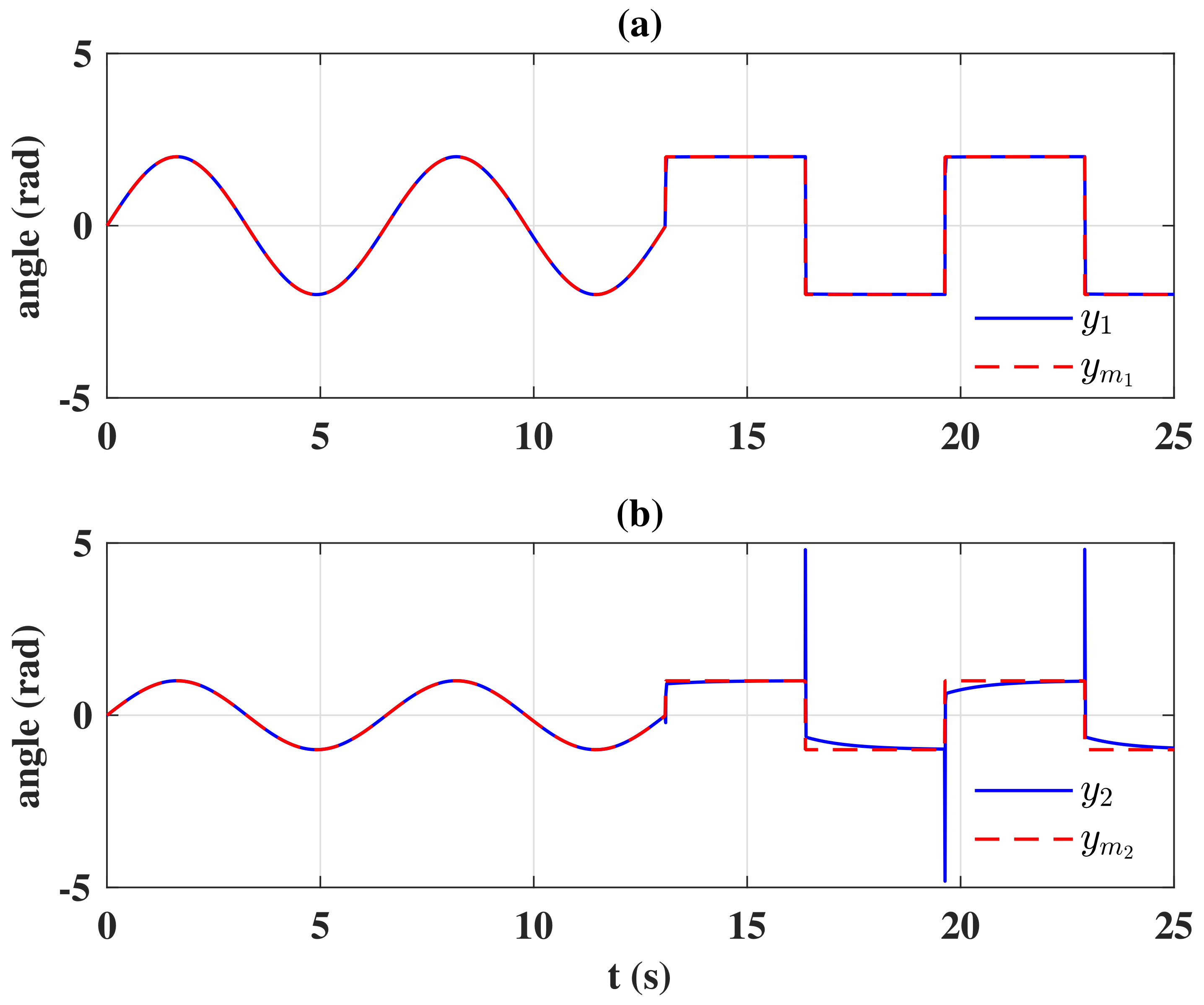
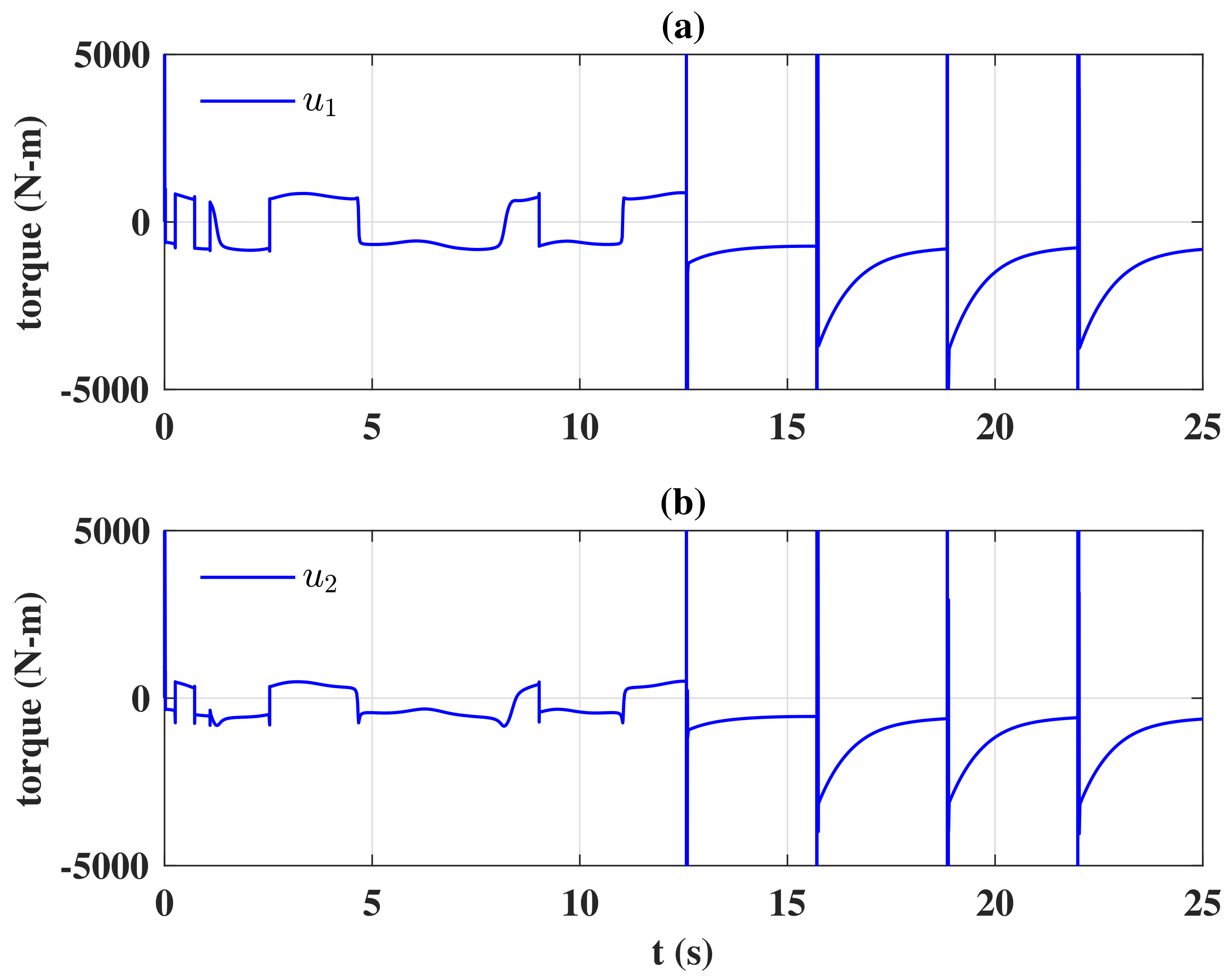
In order to provide a more complete set of validation experiments, the reference signal was extended as:

$$\begin{array}{c}\hfill y_m=\left[\begin{array}{c}{y}_{m_1}\\ y_{m_2}\end{array}\right]=\left\{\begin{array}{c}\left[\begin{array}{c}2sin\left(t\right)\\ sin\left(t\right)\end{array}\right],t\in [0,4\pi )\hfill \\ \\ \left[\begin{array}{c}2\\ 1\end{array}\right],t\in [4\pi ,5\pi ),[6\pi ,7\pi )\hfill \\ \\ \left[\begin{array}{c}-2\\ -1\end{array}\right],t\in [5\pi ,6\pi ),[7\pi ,25],\hfill \end{array}\right.\end{array}$$

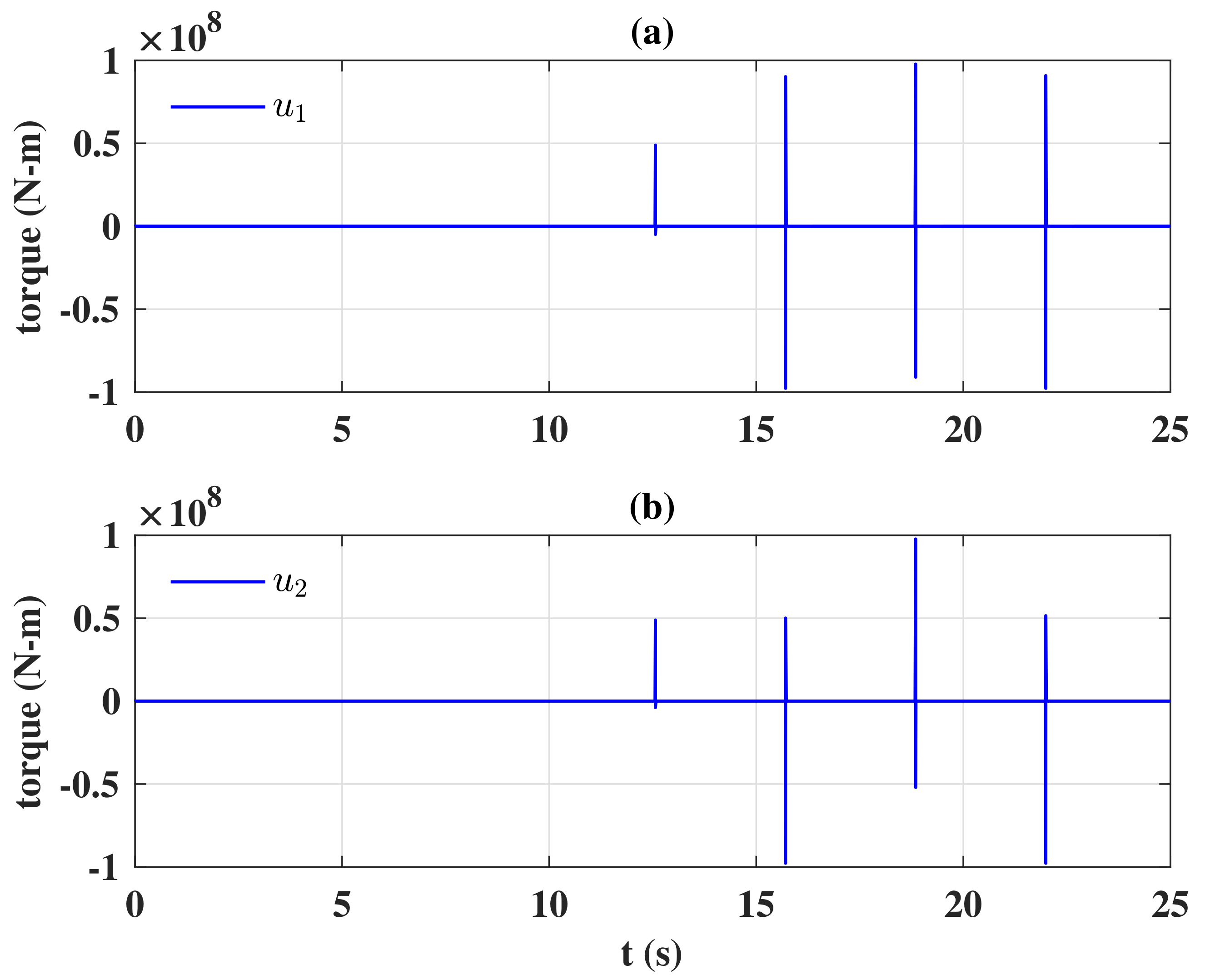
and the control design (35) was applied with the switching gains $c_1=7000$ and $c_0=3000$ in (22). The tracking performance is depicted in Figure 6, and Figure 7 presents the two control signals. In Figure 6, the desired references had discontinuities at $t=4\pi ,5\pi ,6\pi ,7\pi$, and system outputs, especially $y_2$, had a sudden jump at these moments. Likewise, the control signals in Figure 7 inevitably peaked at the time of discontinuities even if the smooth boundary layer control design (35) was implemented. According to (33), $\parallel x_e\parallel \to 0$ when $\xi$ was sufficiently large, and $\parallel {\tilde{x}}_e\parallel =\parallel x_e-{\widehat{x}}_e\parallel \to 0$ according to (13). Consequently, $\parallel {\widehat{x}}_e\parallel \to 0$, and the steady-state of control input (35) was approximated as:

$$\begin{array}{c}\hfill u=-K{\widehat{x}}_e-\rho \left({\widehat{x}}_e\right)\frac{\widehat{\sigma }}{\parallel \widehat{\sigma }\parallel +0.001}\approx -c_0\frac{\widehat{\sigma }}{0.001}.\end{array}$$

(36)

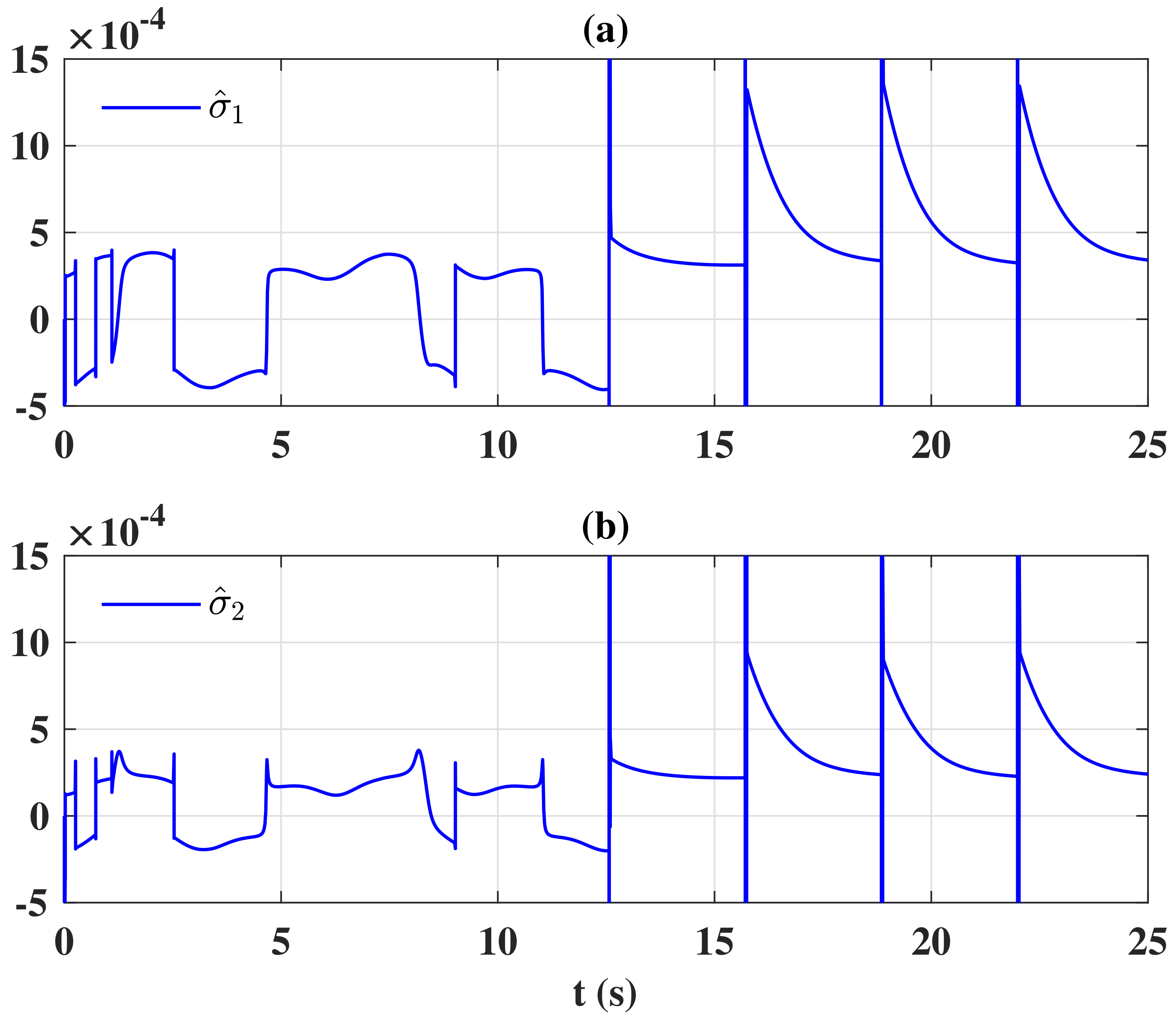
In Figure 8, the time history of the sliding variable is depicted, and the detail of control signal u is shown in Figure 9. In these figures, the approximation of the control signal (36) was confirmed with $c_0=3000$.

Remark 6.

According to (34), it was straightforward to derive the steady-state of input torque signal as:

$$\begin{array}{c}\hfill \tau =G\left(q_m\right)\end{array}$$

when the desired reference $q_m$ was constant. However, the system matrix $G\left(q\right)$ was assumed to be uncertain, and a robust control design (35) was proposed to suppress the unknown nonlinearity. In the sequel, the steady-state of control input (36) therefore depended on the switching gain (22) assigned by the user as in (36).

6. Conclusions

This paper presented an output feedback tracking sliding mode control approach for uncertain linear MIMO systems with uncertainties such as external disturbance, the system state, and control input. In this study, the tracking control problem was first transformed into a stabilizing control problem through the introduction of a reference model for the reference output. Subsequently, a new property of the LTR observer was established; it was revealed that the state estimation error of the LTR observer could be made arbitrarily small with respect to the system uncertainties. Finally, in this paper, observer-based output feedback tracking sliding mode control based on an LTR observer was proposed. The proposed sliding mode control can maintain the boundedness of the system state and drive the system output to track a desired reference output with any degree of accuracy, as determined by a design parameter in the LTR observer. The approach was applied to the case of a two-link robot to illustrate the efficiency of the control design, and a modified controller was presented to remove the harmful chattering and peaking phenomenon for the actuators.