Dynamic Modeling and Control of Antagonistic Variable Stiffness Joint Actuator

Abstract

This study aims to develop a novel decoupling method for the independent control of the position and stiffness of a variable stiffness joint actuator (VSJA), which has been proven to be able to vary its stiffness in a larger range than other variable stiffness actuators. Using static analysis and the Jacobian matrix, we obtained the model of the stiffness of the robot joint actuator and dynamics. Based on the hybrid dynamic model of position and stiffness, it is possible to compensate for the torque of the variable stiffness joint actuator (VSJA) to enhance position control. Finally, after describing the actuator prototype, the established compliance control method is verified using simulation and experimental analysis.

1. Introduction

Variable stiffness robot joints (VSJs) are a class of joints that differ from traditional rigid robot joints in the sense that they are flexible and can adjust their flexibility. Owing to their adjustable stiffness, they can ensure stable contact and safe operation. Therefore, these joints have been integrated into the development of several robots [1,2,3,4,5,6]. Some VSJ [7,8,9,10] have an antagonistic structure that is resemblant to the system of skeletal muscles that regulates stiffness and position in humans. In these, it is possible to separate a drive unit, a variable stiffness mechanism, and an output link. Such separation can significantly reduce the mass and inertia of the output link. It is well-known from the literature [11,12] that the variable stiffness capability of antagonistic structures is directly related to the output torque of the drive units. Therefore, the range of variable stiffness can be small when the torque provided by the motor is limited. In this study, we use a novel permanent magnet mechanism, already presented in [8], which increases the variable stiffness range without increasing the driving torque requirements.

However, introducing compliance to robot joints poses control problems, which have been extensively investigated [13,14,15]. The main motor controls the position or velocity in the traditional series variable stiffness joint. Stiffness is regulated by another auxiliary motor with a variable stiffness mechanism. Stiffness control and position control are independent. Therefore, the challenges linked to the position control problem, associated with mechanical compliance, are mainly related to the control of the main actuator. Previous studies used feedback linearization to control joints with constant compliance or with variable stiffness [16,17,18,19,20]. However, the control problem associated with the compliance of the wire-driven antagonistic VSJs is related to both motors, where a coupling of the joint compliance and position is present [21,22,23,24,25,26]. If the coupling is not dealt with, the control system is often fragile and not anti-disturbance. When the load changes or is subjected to an unknown shock load, problems such as instability of the control system become more prominent [27,28,29,30,31].

In this study, the VSJA is introduced based on the parallel configuration and permanent magnetic mechanism. The actuator stiffness model is obtained using the Jacobian matrix and the static relationship. The nonlinear equations composed of the mechanical model and the stiffness model are solved using the optimization method, which can be used to realize a nonlinear decoupling of the stiffness and position of the actuator, thus independently achieving position and stiffness control and unity of the compliance. Based on the hybrid dynamic model of VSJA’s position and stiffness, a torque observation method was proposed to realize the torque compensation, improving the position control ability under different joint stiffness. The above control method is simple, easy to implement, and practice.

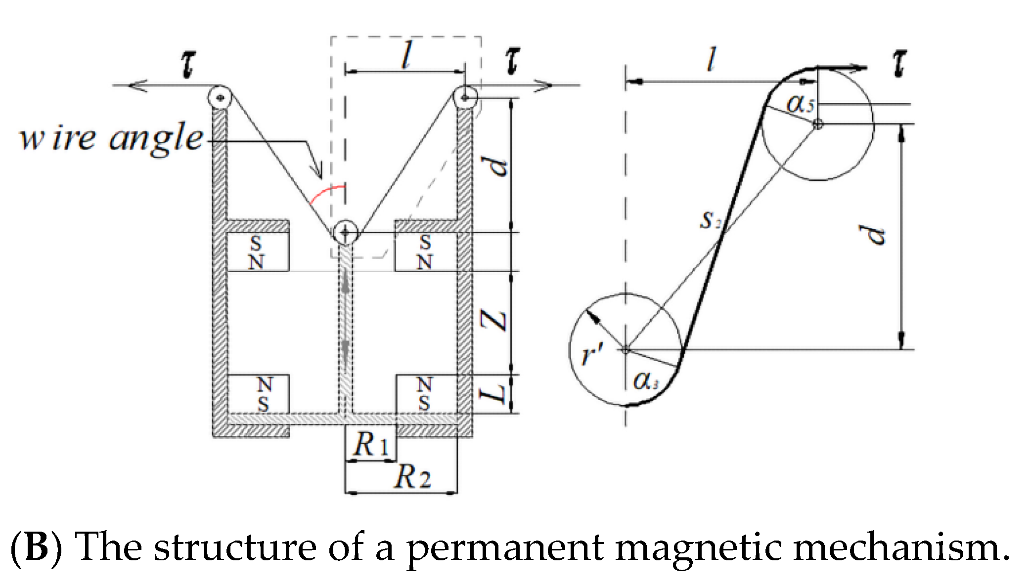
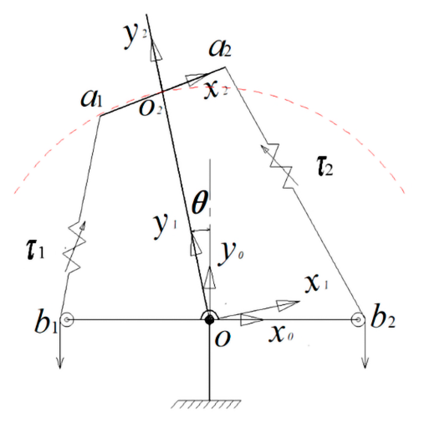
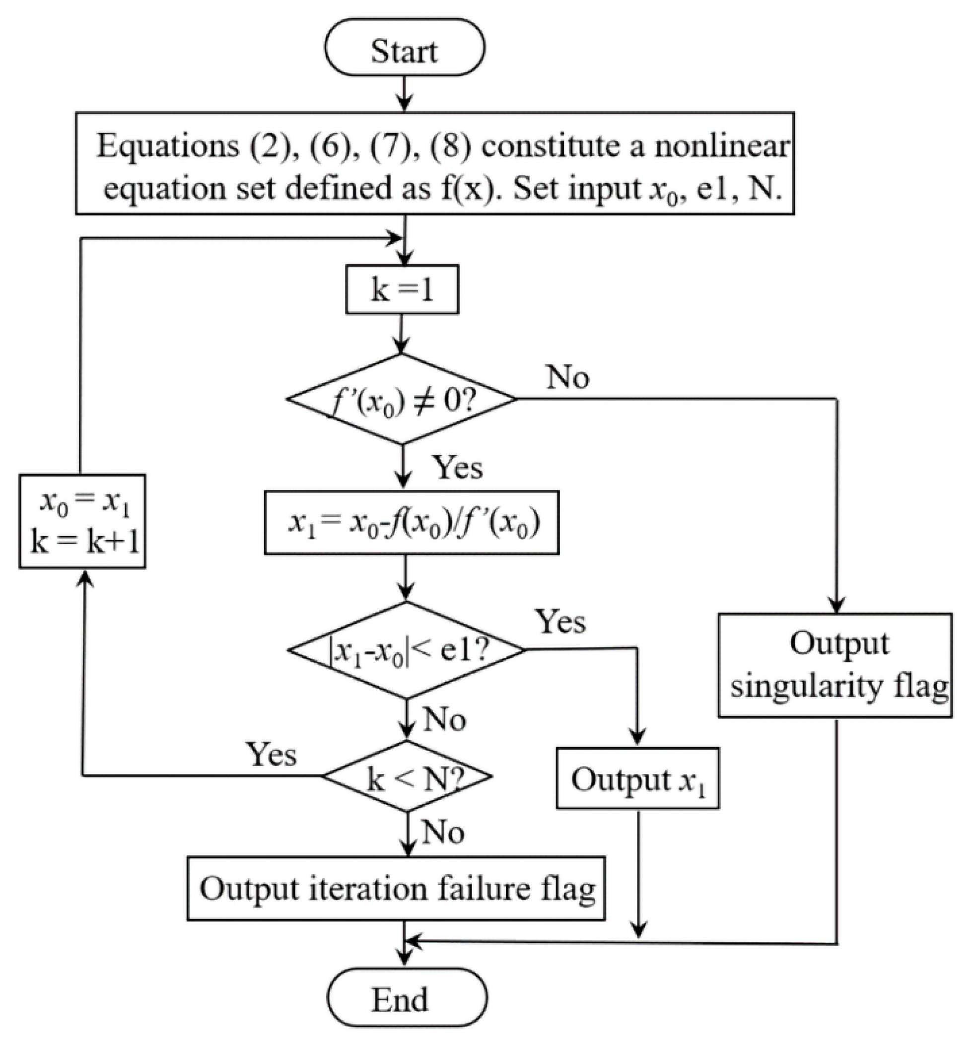
2. Working Principle and Stiffness Model

The VSJA is a parallel wire-driven structure similar to the antagonistic muscle drive-form, as shown in Figure 1A. The permanent magnetic mechanism consists of the permanent magnetic spring module and the wire-driven system [8], which can perform human-like flexible motions. The permanent magnetic spring module comprises of two same-annular permanent magnets, whose similar magnetic poles face each other as shown in Figure 1B. The wire-driven system is used for the VSJA drive. One end of the wire is fixed on one side of the output link through two fixed pulleys and a movable pulley in the permanent magnetic mechanism, while the other end of the wire is fixed on the wire winch of the servomotor. Two groups of the above structures are symmetrically arranged on both sides of the output link. The wire tension τ is applied to the movable pulley through the wire, then the air gap of the magnetic spring module decreases as the movable pulley is pulled up. The magnetic force and stiffness increase nonlinearly when the air gap decreases. The magnetic force acts on the output link through the wire, thus the increase of the magnetic force will increase the stiffness of the joint. A permanent magnet spring was used instead of a linear spring, increasing the variable stiffness performance without increasing the wire tension, unlike the wire-pulley system with a linear spring [14]. Therefore, the joint quality, inertia, and motor power can be reduced. When the two motors rotate in the same direction at a certain speed, the joint position can be changed without changing the stiffness. When the two motors rotate in opposite directions with a certain speed, the joint stiffness can be changed, and the position remains unchanged. The output link is rotated along the output shaft synchronously pulled by the wire. The encoder and output shaft are coaxial. The encoder can be used to determine the real-time position of the output link, evaluating the output link stiffness.

The VSJA coordinate is defined as shown in Figure 2. The coordinate system O₁{x₁, y₁} is fixed at one end of the output link, and the output link is coaxial with the y₁ axis of the O₁{x₁, y₁}. The z₁ axis of the coordinate system O₁{x₁, y₁} and the z₀ axis of the base coordinate system O₀{x₀, y₀} are coaxial. The coordinate system O₂{x₂, y₂} is set on another end of the output link gained by moving coordinate system O₁{x₁, y₁} a definite distance with the y₁ axis. In this coordinate system, the transformation relationship from the output link coordinate system to the base coordinate system can be described through homogeneous transformation. The wire length equation can be obtained.

$$l_i=\Vert \mathrm{rot}\left(z,\theta \right)\mathrm{trans}\left(0,H\right)\cdot P_{a_i}-P_{b_i}\Vert ,i=1,2$$

(1)

In the formula, P_ai is the position vector of the a_i point in coordinate system O₂{x₂, y₂}, and P_bi is the position vector of the b_i point in base coordinate system O₀{x₀, y₀}.

The gravitational force of the output link mg and all wire-tensions τ_j (j = 1~2), have the following static balanced relationship:

$${\displaystyle \sum _{j=1}^2{\tau }_j}\times r_j-mg\times r_g=0,j=1,2$$

(2)

where r_j is the moment arm of the jth wire-tension and r_g is the moment arm of the gravitational force.

Suppose that the joint actuator experiences an infinitesimal external torque ΔT, bringing a tiny variation in the joint actuator Δθ as follows:

$$\frac{\Delta T}{\Delta \theta }=K_{\theta }={\displaystyle \sum _{j=1}^2\left(\frac{\partial {\tau }_j}{\partial \theta }\times r_j+{\tau }_j\times \frac{\partial r_j}{\partial \theta }\right)}-mg\times \frac{\partial r_g}{\partial \theta }$$

(3)

ΔT/Δθ represents the stiffness of actuator K_θ. Representing the length of the jth wire as l_j, ∂τ_j/∂θ is expressed by the following equation:

$$\frac{\partial {\tau }_j}{\partial \theta }=\frac{\partial {\tau }_j}{\partial l_j}{\eta }_j\frac{\partial l_j}{\partial \theta }=k_j{\eta }_j\cdot z_j$$

(4)

K_j = ∂τ_j/∂l_j denotes the stiffness of the permanent magnetic mechanism, ∂l_j/∂θ is expressed by z_j, and η_j represents the vector direction of wire tension τ_j.

The relationship between wire velocity $\dot{l}={\left[{\dot{l}}_1{}_{}{\dot{l}}_2\right]}^T$ and output link velocity $\dot{\theta }$ can be rewritten as (4):

$$\dot{l}=J\dot{\theta }$$

(5)

J represents the Jacobian matrix from $\dot{\theta }$ to $\dot{l}$, which can be expressed by the following equation:

$$J=\left[\begin{array}{c}\frac{R^{\prime }(r\sin \theta -H\cos \theta )}{\sqrt{{R^{\prime }}^2+r^2+H^2-2R^{\prime }(r\cos \theta +H\sin \theta )}}\\ \frac{-R^{\prime }(r\sin \theta +H\cos \theta )}{\sqrt{{R^{\prime }}^2+r^2+H^2-2R^{\prime }(r\cos \theta -H\sin \theta )}}\end{array}\right]$$

(6)

where $\left|o_2{a}_i\right|=r$, $\left|o_2{o}_1\right|=H$ and $\left|o_1{b}_i\right|=R^{\prime }$, i = 1~2.

The relationship between stiffness k₁, k₂ of the permanent magnetic mechanism, and output link stiffness K_θ can be obtained by simplifying Equations (3), (5) and (6) as follows:

$$K_{\theta }=J^{\mathrm{T}}\left[\begin{array}{cc}{k}_1& \\ & k_2\end{array}\right]J$$

(7)

The best-fit mechanical model of wire tension τ(Δl) and wire stretch Δl of the permanent magnet variable stiffness mechanism in [8] was obtained as follows:

$$\tau (\Delta l)=0.0022\Delta l^4-0.0198\Delta l^3+0.0932\Delta l^2+0.3204\Delta l+1.5541$$

(8)

3. Joint Actuator Dynamic Model and Controller Design

The dynamic model of the flexible variable stiffness joint is mainly divided into three parts, including the output link, motor M₁, and motor M₂. The output link is non-linearly coupled, and the motor is linearly decoupled. The variable stiffness mechanism causes the elastic deformation of the joint, and the elastic deformation of the wire is ignored.

$$\{\begin{array}{c}{I}_M\left[\begin{array}{c}{\ddot{\theta }}_1\\ {\ddot{\theta }}_2\end{array}\right]+\left[\begin{array}{c}{r}_d{\xi }_1\\ r_d{\xi }_2\end{array}\right]=\left[\begin{array}{c}{T}_{m1}\\ T_{m2}\end{array}\right]\\ I_L\ddot{\theta }+B_L\dot{\theta }+G(\theta )-J^T\xi =0\end{array}$$

(9)

where I_L is the moment of inertia of the output link, B_L is the damping coefficient of the output link, G(θ) is the gravitational moment vector, I_M is the moment of inertia of the drive unit (including the motor, reducer, winch, etc.) transferred to the motor shaft, r_d is the radius of the winch, and θ_1,2 is the position vector of the 2 × 1 motor rotation angle. When the output link is at the initial position, θ_1,2 is 0. ξ is the tension vector of the wire. T_m is the motor output torque vector. Although there are six state variables θ, $\dot{\theta }$, θ₁, ${\dot{\theta }}_1$, θ₂,${\dot{\theta }}_2$ in the system, only two are independent, and the remaining state variables are determined by θ, $\dot{\theta }$ and stiffness K_θ of the output link.

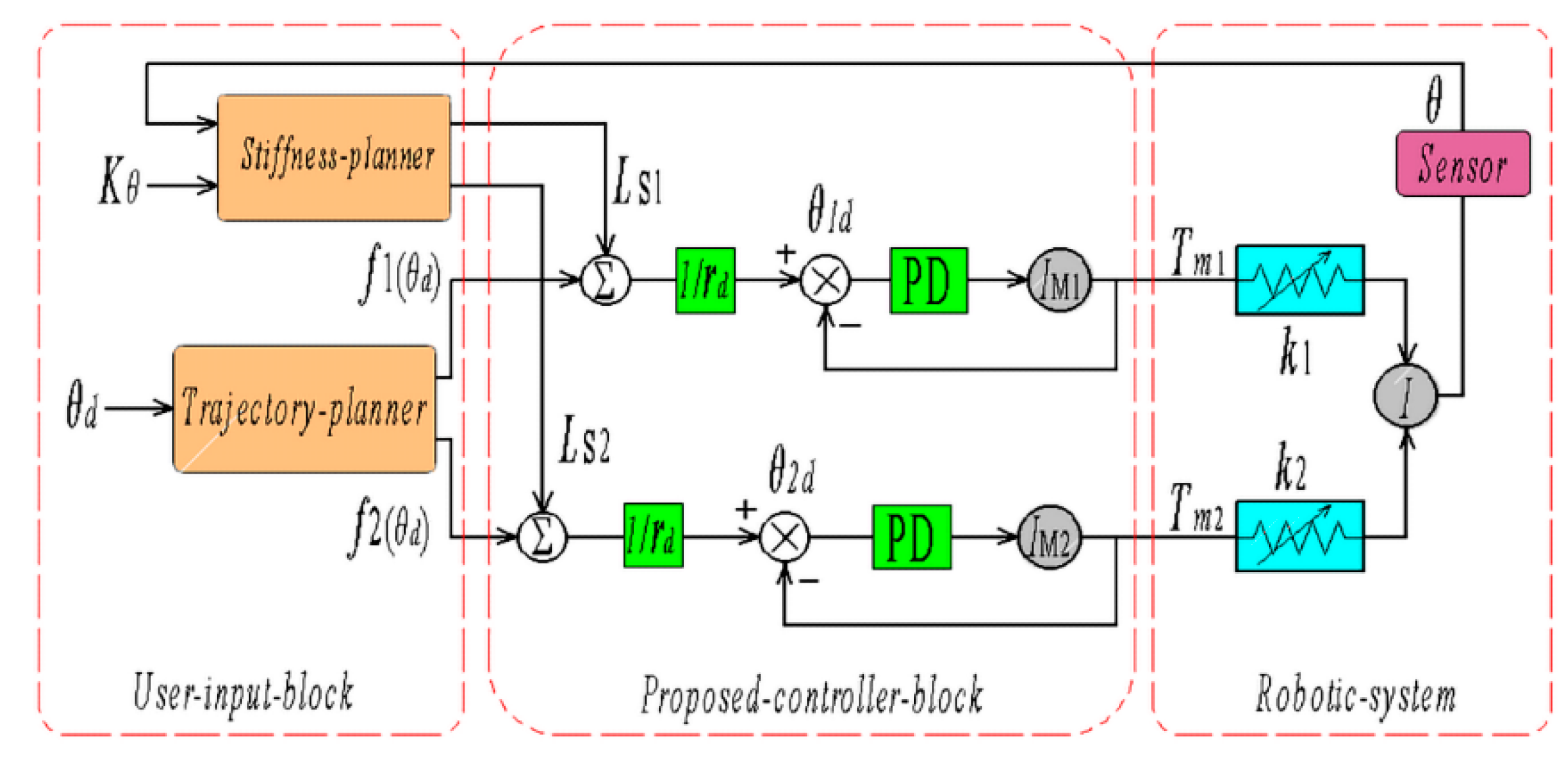
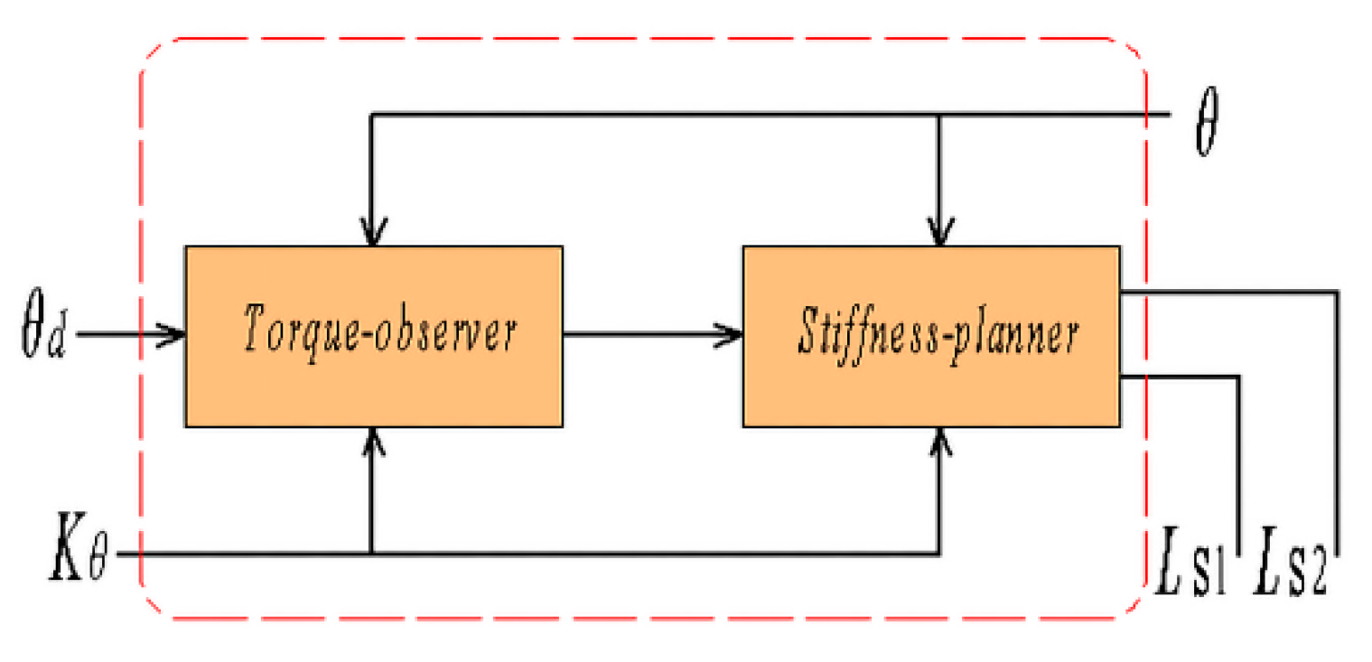
3.1. Controller Design

The gravity moment G(θ) was considered during the solving of the nonlinear equations with the Newton method to realize the stiffness decoupling control. The total input torque is $J^T{[{\xi }_1{}_{}{\xi }_2]}^T-G(\theta )$, the reference input stiffness is K_θ and the input position of the output link is θ_d. The VSJA can be reduced to a physical model consisting of the input torque, the output link, and the elastic part. The input position is θ_d, and the input torque acts on the elastic part first. Then, the torque transmitted to the output link, i.e., the actual output of the output link, is θ, as shown in Figure 3.

The input torque, gravity moment G(θ), and the elastic part have the following balance relationship:

$$J^T{\left[\begin{array}{cc}{\xi }_1& {\xi }_2\end{array}\right]}^T-G(\theta )=K_{\theta }\left({\theta }_d-\theta \right)$$

(10)

Then, the nonlinear dynamic equation of the VSJA can be simplified as follows:

$$I_L\ddot{\theta }+B_L\dot{\theta }=K_{\theta }({\theta }_d-\theta )$$

(11)

Following Laplace transformation of the above formula, the system transfer function is obtained as:

$$\frac{\theta }{{\theta }_d}=\frac{K_{\theta }}{I_L{s}^2+B_{L}s+K_{\theta }}$$

(12)

All the poles of the characteristic root of the system have negative real parts, making the system stable.

In the trajectory planner, the wire length change value fi(θ) that is used to control output link position θ can be obtained.

$$fi(\theta )=\Vert l_{i,0}-l_{i,\theta }\Vert ,i=1,2$$

(13)

Output link position θ and stiffness K_θ are given before calculating Equations (2), (7) and (8), and then the corresponding wire stretch values (L_s1 and L_s2) that realize the output link stiffness can be acquired (Figure 4).

The gravitational force of the output link was considered while determining the values of wire length. This did not require adding the gravity compensation again when controlling the stiffness and position of the output link. The controller of motor M₁ and M₂ are the conventional PD controllers used to regulate the wire length.

$$\{\begin{array}{c}{I}_M\left[\begin{array}{c}{\ddot{\theta }}_1\\ {\ddot{\theta }}_2\end{array}\right]+\left[\begin{array}{c}{r}_d{\xi }_1\\ r_d{\xi }_2\end{array}\right]=\left[\begin{array}{c}{k}_{mp1}({\theta }_{1d}-{\theta }_1)+k_{md1}({\dot{\theta }}_{1d}-{\dot{\theta }}_1)+r_d{\xi }_1\\ k_{mp2}({\theta }_{2d}-{\theta }_2)+k_{md2}({\dot{\theta }}_{2d}-{\dot{\theta }}_2)+r_d{\xi }_2\end{array}\right]\\ I_L\ddot{\theta }+B_L\dot{\theta }=K_{\theta }\left({\theta }_d-\theta \right)\end{array}$$

(14)

The controllers are used to control the actual rotation of the motors. The input term is the sum of the angle required to control the position of the output link and the angle needed to control the stiffness of output link θ_1d and θ_2d. The output term is the actual rotation angle of the motors θ₁ and θ₂.

After Laplace transformation, the closed-loop transfer function of the motor is obtained as:

$$G_M(\mathrm{s})=\frac{k_{d}s+k_P}{I_M{s}^2+k_{d}s+k_p}$$

(15)

To make the system stable, the value ranges of k_d and k_p can be obtained following the Routh-Hurwitz criterion.

The system adopts a position and stiffness hybrid control strategy. The structural block diagram is shown in Figure 5. Given the position of output link θ_d, the rigid parallel robot’s position transformation relationship is used to obtain the wire-length changes f1(θ_d) and f2(θ_d) that are caused by changing the output link’s position. Given the output link stiffness K_θ, using the Newton method to solve the nonlinear equations formed by Equations (2), (7) and (8), the corresponding L_s1 and L_s2 can be obtained. Then, the change in length of the two wires at this time is f1(θ_d) + L_s1 and f2(θ_d) + L_s2, realizing the decoupling control of position and stiffness. Two servo drive motors adopt PD position control. The above-mentioned decoupling controller entirely considers the difference in flexibility when the output link stiffness changes and realizes the position control accuracy and also realizes the stiffness control. This method is simple, easy to implement, and practical.

Next, when the output link is subjected to external torque T_ext, the dynamic equation of the output link becomes:

$$I_L\ddot{\theta }+B_L\dot{\theta }+T_{ext}=K_{\theta }\left({\theta }_d-\theta \right)$$

(16)

Then the final steady-state form of the system becomes:

$$T_{ext}=K_{\theta }\left({\theta }_d-\theta \right)$$

(17)

It can be seen from the final stable form of the system that as long as the stiffness of the joint is controlled accurately, compliance can be adjusted accurately.

When the output link is subjected to an external torque, the new balance relationship is formed as follows:

$${\displaystyle \sum _{j=1}^2{\xi }_j}\times r_j-mg\times r_g=T_{ext},j=1,2$$

(18)

From Equation (14), the external torque T_ext can be estimated. Solving the new nonlinear equations formed by Equations (7), (8) and (18), and obtaining new wire-length changes L_s1 and L_s2, the compensation of gravity and compensation of external torque can be realized, as shown in Figure 6. The advantage is that when an external force deforms the output link, it can be detected by the encoder in real-time, and then substituted into the decoupling calculation.

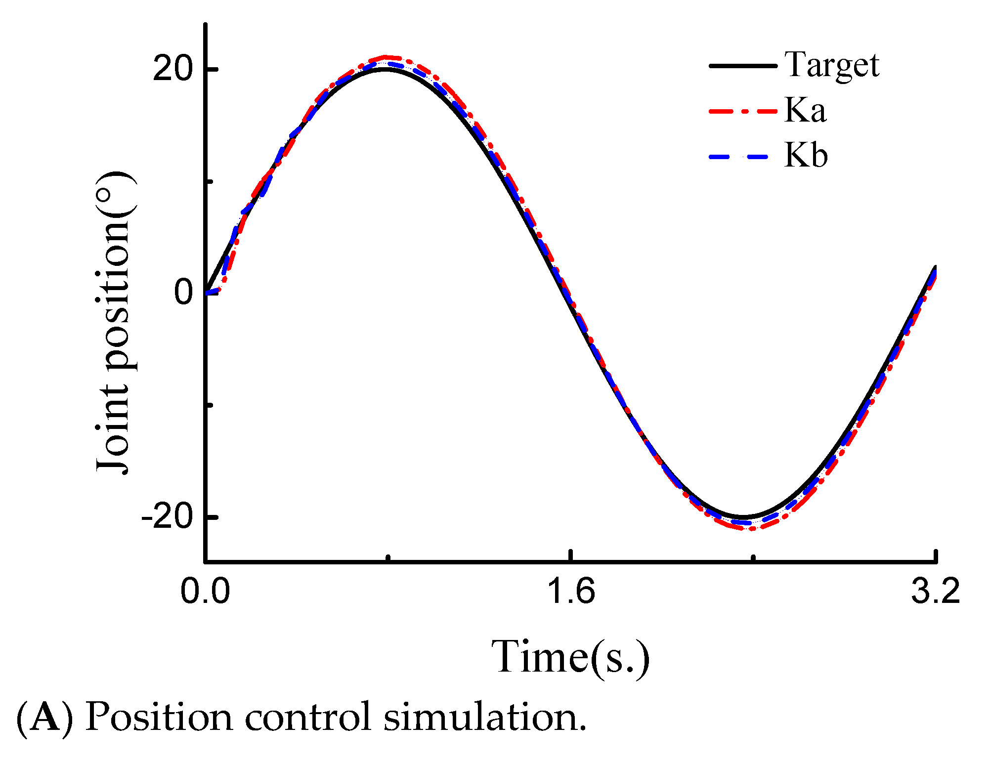
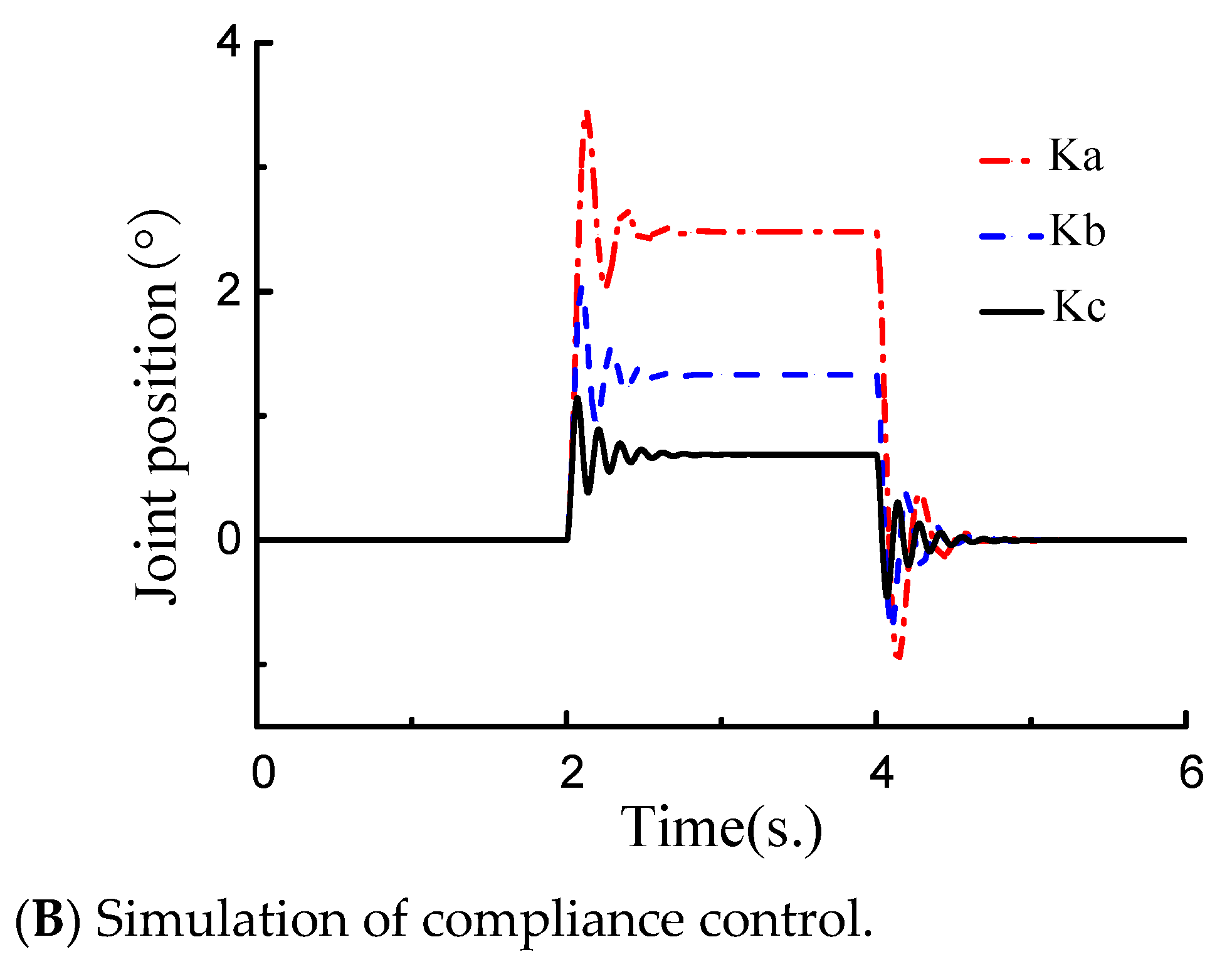
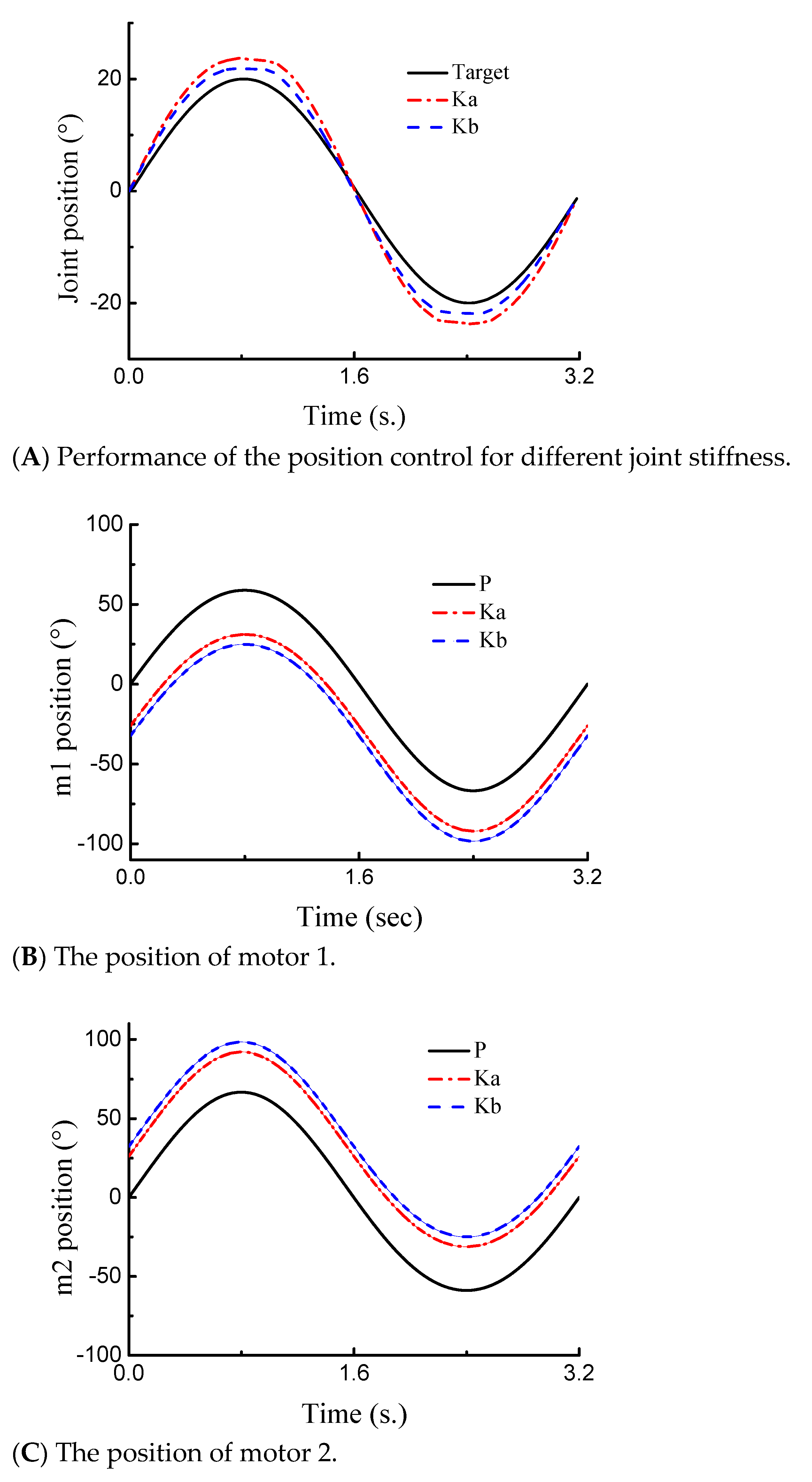
3.2. System Simulation Analysis

The structural parameters of the variable stiffness joint actuator are as shown in

Table 1. Datasheet of the joint actuator.

Mechanical Specification	Value	Unit
Stiffness range	0~∞	[N·m/rad]
Time for stiffness change	0.4	[s]
Range of joint rotation	140	[°]
Dimensions o2a1 = o2a2	0.024	[m]
oo2	0.072	[m]
ob1 = ob2	0.08	[m]
Winch radius rd	0.02	[m]
Winch inertia IM	0.0002	[kg·m2]
Output link inertia IL	1.2	[kg·m2]
Output link weight m	0.3	[kg]
Output link length L	0.25	[m]

. Using the S-Function module in MATLAB/Simulink for simulation analysis, we substituted the corresponding parameters of the joint actuator into the simulation block diagram.

The simulation result of the relationship between the joint position response and joint stiffness change is shown in Figure 7A. The stiffness of the VSJA was changed to Ka = 30 N·m/rad and Kb = 60 N·m/rad. Then, a sine signal with an amplitude of 20 degrees and a period of 3.2 s was given to the VSJA. The position response of the VSJA is as shown in Figure 7A. The dotted-and-dashed red line was the trajectory following the VSJA, when joint stiffness Ka = 30 N·m/rad. The dashed blue line was the trajectory following the VSJA, when joint stiffness Kb = 60 N·m/rad. The law of the change between position response and joint stiffness can be obtained from the simulation results. When the joint stiffness was low, the position error of the VSJA caused by inertia was large, and the position error was bigger than high joint stiffness. Meanwhile, with the increase in joint stiffness, the position error caused by inertia was suppressed.

The simulation result of the VSJA’s compliance is shown in Figure 7B. When the VSJA was in the initial position, the stiffness of the VSJA was changed to Ka, Kb and Kc (Ka = 30 N·m/rad, Kb = 60 N·m/rad and Kc = 90 N·m/rad). In the time period of 2 to 4 s, an external torque of 1.5 Nm was applied to the VSJA, the position change of the VSJA is shown in Figure 7B. When the joint stiffness is Ka, the joint position change is shown as a dotted-and-dashed red line. When the joint stiffness is Kb, the change in joint position is shown as a dashed blue line. When the joint stiffness is Kc, the change in joint position is shown as a solid black line. By analyzing the relationship between joint position and stiffness change, we found that the accurate control of VSJA compliance can be achieved through the change in joint stiffness.

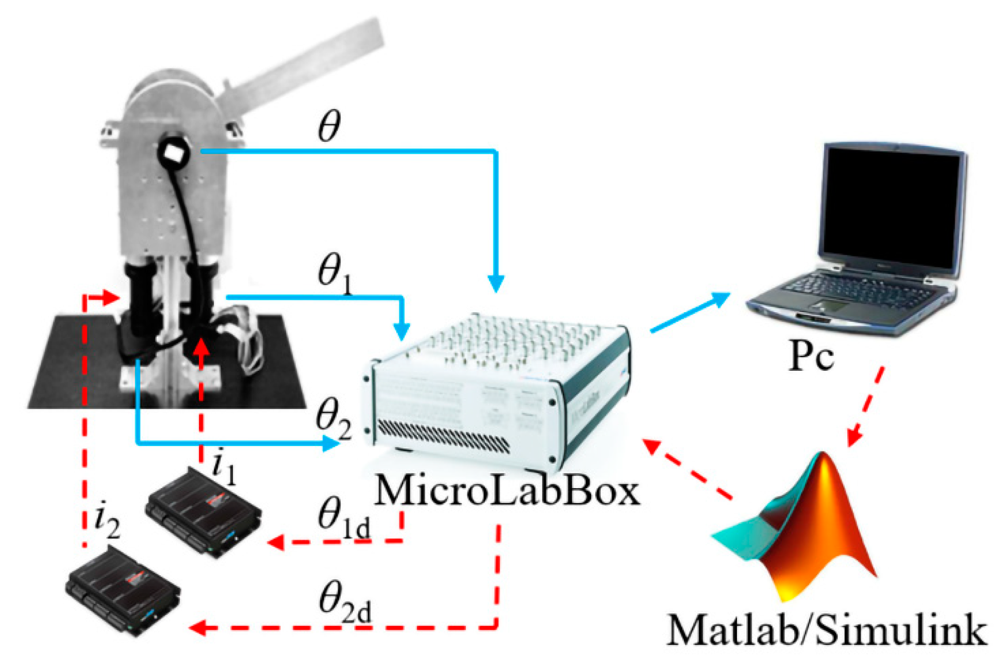
4. Experimental Analysis

The experimental setup, using a wire-driven variable stiffness robot joint actuator, was constructed as shown in Figure 8. The controller unit of the variable stiffness robot joint actuator was a MicroLabBox (MicroLabBox, dsPACE, Paderborn, Germany), regulating the motions of DC servo motors (M1 and M2) with the harmonic reducer (the reduction ratio is 50:1) at 1 kHz. The joint actuator control code was written directly in the real-time control software MATLAB/Simulink (2012).

4.1. Analysis of Position Control

To investigate the performance of the position control, sine signals with an amplitude of 20 degrees and a period of 3.2 s were investigated for different joint stiffness values. The motion direction of the joint actuator was perpendicular to the gravity direction. The dotted-and-dashed red lines represent the measured joint position for joint stiffness Ka (Ka = 30 N·m/rad), and the dashed blue lines represent the joint position for joint stiffness Kb (Kb = 60 N·m/rad), as shown in Figure 9A. This experimental result demonstrated the behavior of a compliant joint. As the joint stiffness increased, the overshoot decreased, and the response speed increased. The deviations at the peak position and valley position were higher than those in the other position. The corresponding DC servo motor (M1 and M2) rotations are shown in Figure 9B,C. The solid black line represents the theoretical motor rotation when only controlling the joint position. When controlling the joint stiffness, the two motors rotated in opposite directions. When controlling the joint position, the two motors rotated in the same direction. By adjusting the angle of the motor, the stiffness and position of the joint could be controlled independently.

4.2. Analysis of Compliance Control

A weight of 0.25 kg, with a 200 mm vertical height, affected the output link end of the variable stiffness joint actuator whose length was 250 mm. Meanwhile, the deflection angle of the variable stiffness joint actuator was recorded. The initial condition was that the output link of the joint actuator remained horizontal, and no external torque was applied to it. When the stiffness of the variable stiffness joint was Ka = 30 N·m/rad, Kb = 60 N·m/rad, and Kc = 90 N·m/rad, we repeated the collision experiment and recorded the maximum deflection angle and vibration time. As shown in Figure 10, when the stiffness of the variable stiffness joint was Ka, the maximum deflection angle (−8.49°) of the output link was much bigger than joint stiffness Kb (−6.48°) and joint stiffness Kc (−5.4°). When stiffness was at a higher level, the vibration was slight, and the vibration time was about 0.23 s. However, when stiffness was at a lower level, vibration was significant, and the vibration time (0.35 s) was much longer. The experiments demonstrated that vibration and vibration time increased with the decrease in joint stiffness.

The safety of the variable stiffness joint actuator was verified using collision experiments. The collision force between the output link end and the weight can be calculated by the maximum deflection angle and corresponding joint stiffness, as shown in Figure 10. The maximum collision force at stiffness level Ka was 4.44 N at the time of 0.477 s. The maximum collision force at stiffness level Kb was 6.78 N at the time of 1.278 s. The maximum collision force at stiffness level Kc was 8.48 N at the time of 2.057 s. The collision condition of the experiment was the same, and the collision force can be regulated easily by changing the stiffness of the variable stiffness joint actuator. This means that the variable stiffness joint can effectively absorb the collision force by changing the joint’s stiffness.

4.3. Analysis of Force Compensation

To investigate the control performance of the compensation of the external torque, a 0.5 kg weight was attached to the output link (length of 250 mm), to observe the deformation angle of the variable stiffness joint actuator using controller I (decoupling controller) and controller II (decoupling controller with compensation of external torque), respectively. The experiment was repeated at two joint stiffness levels, and the results are as listed in

Table 2. Deformation angle of variable-stiffness joint.

Weight (kg)	Stiffness (Nm/rad)	Compensation	Average Deflection Angle (°)	Each Deflection Angle (°)
0.5	30	No	3.32	3.4 3.2 3.3 3.4 3.3
0.5	30	Yes	0.32	0.3 0.4 0.3 0.2 0.4
0.5	60	No	1.58	1.7 1.6 1.6 1.5 1.5
0.5	60	Yes	0.28	0.4 0.3 0.3 0.2 0.2

. When the joint stiffness was 30 N·m/rad, using controller I, the average deformation angle of the variable stiffness joint was 3.32°, while using controller II, the average deformation angle was 0.32°. When the joint stiffness was 60 N·m/rad, using controller I, the average deformation angle of the variable stiffness joint was 1.58°, while using controller II, the average deformation angle was 0.28°. These results showed that the decoupling controller with an external force compensation could significantly improve the position control accuracy for the variable stiffness joint. The stiffness control effect of the decoupling controller can meet the working requirements, and the external force compensation link can be selected according to the position control accuracy requirements.

5. Conclusions

Aiming at the stability and safety of the interaction between users and robots, this study proposed a decoupling control method for the position and stiffness for the wire-driven variable stiffness robot joint actuator, realizing compliance control and position control. The joint actuator stiffness model is obtained using the Jacobian matrix and the static relationship between the models. The nonlinear equations composed of the mechanical model of the variable stiffness mechanism and the joint stiffness model were solved using the optimization method to realize a nonlinear decoupling of stiffness and position.

Based on the decoupling control method, the variable stiffness joint actuator torque compensation was realized, and the joint position tracking ability was improved. The joint prototype and control system of the variable stiffness joint actuator was established. The feasibility and effectiveness of the above compliant control and external torque compensation methods were verified via simulation and experimental analysis. The current study lays the foundation for a real-time control system considering dynamic modeling and disturbance uncertainty in the future.

References

1. Vu, H.-Q.; Yu, X.; Lida, F.; Pfeifer, R. Improving energy efficiency of hopping locomotion by using a variable stiffness actuator. IEEE/ASME Trans. Mechatron. 2016, 21, 472–486. [Google Scholar] [CrossRef]
2. Kim, B.-S.; Song, J.-B. Design and control of a variable stiffness actuator based on adjustable moment arm. IEEE Trans. Robot. 2012, 28, 1145–1151. [Google Scholar]
3. Tao, Y.; Wang, T.-M.; Wang, Y.-Q.; Guo, L.; Xiong, H.-G.; Xu, D. A new variable stiffness robotic joint. Ind. Robot. Int. J. 2015, 42, 371–378. [Google Scholar] [CrossRef]
4. Tsagarakis, N.-G.; Sardellitti, I.; Caldwell, D.-G. A new variable stiffness actuator (CompAct-VSA): Design and modelling. In Proceedings of the 2011 IEEE/RSJ International Conference on Intelligent Robots and Systems (IROS), San Francisco, CA, USA, 25–30 September 2011. [Google Scholar]
5. Park, J.; Song, J.-B. Safe joint mechanism using inclined link with springs for collision safety and position accuracy of a robot arm. In Proceedings of the IEEE International Conference on Robotics and Automation (ICRA), Anchorage, AK, USA, 3–7 May 2010; pp. 813–818. [Google Scholar]
6. Fang, L.; Wang, Y. Study on the stiffness property of a variable stiffness joint using a leaf spring. Proc. Inst. Mech. Eng. Part C: J. Mech. Eng. Sci. 2018, 233, 1021–1031. [Google Scholar] [CrossRef]
7. Shah, D.; Wu, Y.-Q.; Scalzo, A.; Metta, G.; Parmiggiani, A. A comparison of robot wrist implementations for the icub humanoid. Robotics 2019, 8, 11. [Google Scholar] [CrossRef] [Green Version]
8. Zhang, M.; Fang, L.-J.; Sun, F.; Sun, X.-W.; Gao, Y.; Oka, K. Realization of flexible motion of robot joint with a novel permanent magnetic spring. In Proceedings of the IEEE International Conference on Intelligence and Safety for Robotics, Shenyang, China, 24–27 August 2018; pp. 331–336. [Google Scholar]
9. Amir, J. Coupling between the output force and stiffness in different variable stiffness actuators. Actuators 2014, 3, 270–284. [Google Scholar]
10. Wang, W.; Zhao, Y.-W.; Li, Y.-M. Design and dynamic modeling of variable stiffness joint actuator based on archimedes spiral. IEEE Access 2018, 4, 43798–43807. [Google Scholar] [CrossRef]
11. Nakanishi, Y.; Ito, N.; Shirai, T.; Osada, M.; Izawa, T.; Ohta, S.; Urata, J.; Okada, K.; Inaba, M. Design and powerful and flexible musculoskeletal arm by using nonlinear spring unit and electromagnetic clutch opening mechanism. In Proceedings of the IEEE-RAS International Conference on Humanoid Robots, Bled, Slovenia, 26–28 October 2011; pp. 377–382. [Google Scholar]
12. Bi, S.-S.; Liu, C.; Zhao, H.-Z.; Wang, Y.-L. Design and analysis of a novel variable stiffness actuator based on parallel-assembled-folded serial leaf springs. Adv. Robot. 2017, 31, 990–1001. [Google Scholar] [CrossRef]
13. Wang, W.; Fu, X.-Y.; Li, Y.-M.; Yun, C. Design of variable stiffness actuator based on modified gear-rack mechanism. Mech. J. Mech. Robot. 2016, 8, 061008. [Google Scholar] [CrossRef]
14. Osada, M.; Ito, N.; Nakanishi, Y.; Inaba, M. Realization of flexible motion by musculoskeletal humanoid “Kojiro” with add-on nonlinear spring units. In Proceedings of the IEEE-RAS International Conference on Humanoid Robots, Nashville, TN, USA, 6–8 December 2010; pp. 174–179. [Google Scholar]
15. Alazmani, A.; Keeling, D.-G.; Walker, P.-G.; Abbas, S.-K.; Jaber, O.; Sivananthan, M.; Watterson, K.; Levesley, M.-C. Design and evaluation of a buckled strip compliant actuator. IEEE/ASME Trans. Mechatron. 2013, 18, 1819–1826. [Google Scholar] [CrossRef]
16. Palli, G.; Melchiorri, C.-J.; Luca, A.-D. On the feedback linearization of robots with variable stiffness. In Proceedings of the IEEE International Conference on Robotics and Automation, Pasadena, CA, USA, 19–23 May 2008; pp. 1753–1759. [Google Scholar]
17. Liu, L.; Leonhardt, S.; Misgeld, B.-J. Design and control of a mechanical rotary variable impedance actuator. Mechatronics 2016, 39, 226–236. [Google Scholar] [CrossRef]
18. Wang, W.; Fu, X.-Y.; Li, Y.-M.; Yun, C. Design and implementation of a variable stiffness actuator based on flexible gear rack mechanism. Robotica 2018, 36, 448–462. [Google Scholar] [CrossRef]
19. Zhou, X.-B.; Jun, S.-K.; Krovi, V. A cable based active variable stiffness module with decoupled tension. J. Mech. Robot. 2015, 7, 011005. [Google Scholar] [CrossRef]
20. Groothuis, S.; Carloni, R.; Stramigioli, S. A novel variable stiffness mechanism capable of an infinite stiffness range and unlimited decoupled output motion. Actuators 2014, 3, 107–123. [Google Scholar] [CrossRef]
21. Torrealba, R.-R.; Udelman, S.-B. Design of cam shape for maximum stiffness variability on a novel compliant actuator using differential evolution. Mech. Mach. Theory 2016, 95, 114–124. [Google Scholar] [CrossRef]
22. Zhakatayev, A.; Rubagotti, M.; Varol, H.-A. Closed-loop control of variable stiffness actuated robots via nonlinear model predictive control. IEEE Access 2015, 3, 235–248. [Google Scholar] [CrossRef] [Green Version]
23. Yu, J.; Zhao, Y.; Wang, H.; Chen, G.; Lai, X. The best-approximate realization of a spatial stiffness matrix with simple springs connected in parallel. Mech. Mach. Theory 2016, 103, 236–249. [Google Scholar] [CrossRef] [Green Version]
24. Chen, P.; Li, H.-Y. A decoupled control method based on MIMO system for flexible manipulators with FS-SEA. In Proceedings of the IEEE Conference on Robotics and Biomimetics, Zhuhai, China, 6–27 December 2015; pp. 662–667. [Google Scholar]
25. Florian, P.; Andreas, D.; Alin, A.-S. Backstepping control of variable stiffness robots. IEEE Trans. Control Syst. Technol. 2015, 23, 2195–2201. [Google Scholar]
26. Zhao, Y.; Yu, J.; Wang, H.; Chen, G.; Lai, X. Design of an electromagnetic prismatic joint with variable stiffness. Ind. Robot. Int. J. 2017, 44, 173–181. [Google Scholar] [CrossRef]
27. Jafari, A.; Tsagarakis, N.-G.; Caldwell, D.-G. A novel intrinsically energy efficient actuator with adjustable stiffness. IEEE/ASME Trans. Mechatron. 2013, 18, 355–365. [Google Scholar] [CrossRef]
28. Braun, D.-J.; Petit, F.; Huber, F.; Haddadin, S. Robots driven by compliant actuators: Optimal control under actuation constraints. IEEE Trans. Robot. 2013, 29, 1085–1101. [Google Scholar] [CrossRef] [Green Version]
29. Xie, H.-L.; Zhao, X.-F.; Sun, Q.-C.; Yang, K.; Li, F. A new virtual-real gravity compensated inverted pendulum model and adams simulation for biped robot with heterogeneous legs. J. Mech. Sci. Technol. 2020, 34, 401–412. [Google Scholar] [CrossRef]
30. Kim, Y.-J.; Kim, J.-I.; Jang, W. Quaternion joint: Dexterous 3-DOF joint representing quaternion motion for high-speed safe interaction. In Proceedings of the IEEE/RSJ International Conference on Intelligent Robots and Systems (IROS), Madrid, Spain, 1–5 October 2018; pp. 935–942. [Google Scholar]
31. Refour, E.-M.; Sebastin, B.; Chauhan, R.-J.; Tzvi, P.-B. A general purpose robotic hand exoskeleton with series elastic actuation. J. Mech. Robot. 2019, 11, 060902. [Google Scholar] [CrossRef] [PubMed]
Figure 1. The variable stiffness robot joint actuator prototype; (A) position control simulation, and (B) the structure of a permanent magnetic mechanism; (1) wire; (2) permanent magnetic mechanism; (3) wire reel; (4) harmonic reducer and DC servo motor with an encoder; (5) Base; (6) Encoder; and (7) output link.
Actuators 10 00116 g001aActuators 10 00116 g001b
Figure 2. Definition of the variable stiffness joint actuator coordinate.
Actuators 10 00116 g002
Figure 3. The physical model of a variable stiffness joint.
Actuators 10 00116 g003
Figure 4. The Newton method to realize nonlinear decoupling calculation.
Actuators 10 00116 g004
Figure 5. Structure of decoupling controller.
Actuators 10 00116 g005
Figure 6. Implementation of torque compensation.
Actuators 10 00116 g006
Figure 7. Simulation results of variable stiffness robot joint; (A) position control simulation, and (B) simulation of compliance control.
Actuators 10 00116 g007aActuators 10 00116 g007b
Figure 8. Experimental setup using a robot joint actuator.
Actuators 10 00116 g008
Figure 9. Sine trajectory tracking. (A) performance of the position control for different joint stiffness; (B) the position of motor 1; (C) the position of motor 2.
Actuators 10 00116 g009
Figure 10. Compliance analysis of variable-stiffness joint.
Actuators 10 00116 g010