A Robust Noise-Free Linear Control Design for Robot Manipulator with Uncertain System Parameters

Abstract

In robot control, the sliding mode control is known for its robustness against external disturbances and system uncertainties. However, it has the disadvantage of control chattering, which can damage the actuator and degrade system performance. With a new stability proof, this paper presents an alternative simple linear feedback control that can cope with large system uncertainties and suppress large external disturbances, doing so as effectively as sliding mode control does. The advantage of using linear control is that the control law is simple and control chattering can be avoided. Moreover, a noise-free control scheme is proposed as an improvement of the feedback control; the modified design preserves the advantages of linear control and generates a chattering-free control signal even in a noisy environment.

1. Introduction

The tracking control of robot manipulators is a mature field but still has many research possibilities, and a straightforward control scheme is known as computed-torque control [1]. Computed-torque control generally performs well in practice when the robot arm parameters are accurately known [1]. When uncertainties and unknown disturbances occur, conventional robust stability analysis shows that if the nominal system is exponentially stable, the system can tolerate “small” system uncertainties and external disturbances [2], therefore restricting the application of linear control to robot manipulators, which is a highly nonlinear system. In this case, adaptive control [3,4,5], sliding-mode control [6,7,8,9,10,11], and neural network control [12,13,14] were proposed to solve the problem.

Sliding mode control is known for its robustness against large system uncertainties and external disturbances [15,16]. However, the sliding mode control has a disadvantage of control chattering, which is due either to switching time delay [17] or unmodelled dynamics [18,19]. Boundary layer design has been proposed as a solution, in which the switching function is replaced with a continuous interpolation function [6,20]. In boundary layer design, control accuracy and control smoothness are ensured by a small and large boundary layer width, respectively, and thus trade off each other.

Other approaches have also been proposed to reduced control chattering in sliding mode control, such as higher-order sliding-mode (HOSM) control [21]. The application of HOSM control to robot manipulator can be found in [22,23,24,25]. However, the modified sliding mode controls are complicated. Moreover, the boundary layer control [26] and HOSM control [27] were proved to be sensitive to measurement noise; the control signal will inevitably have undesired chattering when the state or the estimation is corrupted by a stochastic noise, and only uniformly ultimate boundedness is guaranteed for both designs in a noisy environment.

The purpose of this paper is to demonstrate that simple linear control can deal with system uncertainties and external disturbances as effectively as sliding mode control can, especially in the robot control task. Furthermore, linear control has no side effect of control chattering, and its control law is simple. Disagreeing with the conventional belief that linear control can only cope with small linear or nonlinear system uncertainties [28,29], this paper formulates a framework where linear control can cope with large linear or nonlinear system uncertainties and suppress large external disturbances. With the new stability analysis, the linear control design is proposed as a modified computed-torque control that does not require the information of system parameters. Moreover, a noise-free control scheme is presented to efficiently eliminate the noise-induced chattering that often occurs in sliding-mode [27] of boundary layer controls [26].

The remainder of this paper proceeds as follows. The problem is formulated in Section 2, preliminary lemmas are presented in Section 3, the stability of the proposed linear control is analyzed in Section 4, the noise-free control scheme design is presented in Section 5, an application to a two degree-of-freedom (DOF) robot manipulator is demonstrated in Section 6, and conclusions are presented in Section 7.

2. Problem Description

Consider the dynamic equation of an n-DOF link robot

$$\begin{array}{c}\hfill M\left(q\right)\ddot{q}+C(q,\dot{q})\dot{q}+G\left(q\right)+F\dot{q}=\tau ,\end{array}$$

(1)

where $q={[q_1,\cdots ,q_n]}^T$ is joint position, $\dot{q}$, $\ddot{q}\in R^n$ are the joint velocity and acceleration vectors; $M\left(q\right)$, $C(q,\dot{q})$, $G\left(q\right)$, F are the inertia matrix, Coriolis matrix, gravity matrix, and frictional matrix with proper dimensions, $\tau \in R^n$ is the input torque vector. Defining the desired joint position $q_d={[q_{d_1},\cdots ,q_{d_n}]}^T$, velocity ${\dot{q}}_d$, and acceleration ${\ddot{q}}_d$, the position errors for each joint are given as $e_i=x_i=q_i-q_{d_i}$ for all $i=1\cdots n$, and the error vector $x={[x_1,{\dot{x}}_1,x_2,{\dot{x}}_2,\cdots ,x_n,{\dot{x}}_n]}^T$ is composed. When the system matrices $M\left(q\right)$, $C(q,\dot{q})$, $G\left(q\right)$, F in (1) are accurately known, the computed-torque control [1] gives

$$\begin{array}{c}\hfill \tau =M\left(q\right)({\ddot{q}}_d-Kx)+C(q,\dot{q})\dot{q}+G\left(q\right)+F\dot{q},\end{array}$$

(2)

where

$$\begin{array}{c}\hfill K=\left[\begin{array}{cccc}{\underline{K}}_1& {\varphi }_{1\times 2}& \cdots & {\varphi }_{1\times 2}\\ {\varphi }_{1\times 2}& {\underline{K}}_2& \ddots & ⋮\\ ⋮& \ddots & \ddots & {\varphi }_{1\times 2}\\ {\varphi }_{1\times 2}& \cdots & {\varphi }_{1\times 2}& {\underline{K}}_N\end{array}\right]\in R^{n\times \left(2n\right)}\end{array}$$

(3)

is the gain matrix to be determined with ${\underline{K}}_i=[k_{i_1},k_{i_2}]\in R^{1\times 2}$ for all $i=1,\cdots ,n$, and $\varphi \in R^{p\times q}$ is a $p\times q$ zero matrix. Substituting the torque commend (2) into (1) yields

$$\begin{array}{c}\hfill M\left(q\right)\ddot{e}+K_1\dot{e}+K_{0}e=0,\end{array}$$

(4)

which is the basic formulation of impedance control of a robot manipulator [30] with constant diagonal matrices $K_0=diag(k_{1_1},k_{2_1},\cdots ,k_{n_1})$ and $K_1=diag(k_{1_2},k_{2_2},\cdots ,k_{n_2})$.

When the system matrices $M\left(q\right)$, $C(q,\dot{q})$, $G\left(q\right)$, F in (1) are unknown, the error dynamic of the state vector x is described as

$$\begin{array}{c}\hfill \dot{x}=Ax+B(u+\Delta f\left(x\right)+d)\end{array}$$

(5)

on the basis of (1), where

$$\begin{array}{c}\hfill u\left(x\right)=\tau ,\Delta f\left(x\right)=M^{-1}\left(q\right)(\tau -C(q,\dot{q})\dot{q}-G\left(q\right)-F\dot{q})-\tau ,d=-{\ddot{q}}_d,\end{array}$$

(6)

and the system matrices are

$$\begin{array}{cc}\hfill A& =\left[\begin{array}{cccc}\underline{A}& {\varphi }_{2\times 2}& \cdots & {\varphi }_{2\times 2}\\ {\varphi }_{2\times 2}& \underline{A}& \ddots & ⋮\\ ⋮& \ddots & \ddots & {\varphi }_{2\times 2}\\ {\varphi }_{2\times 2}& \cdots & {\varphi }_{2\times 2}& \underline{A}\end{array}\right]\in R^{\left(2n\right)\times \left(2n\right)},\hfill \\ \hfill B& =\left[\begin{array}{cccc}\underline{B}& {\varphi }_{2\times 1}& \cdots & {\varphi }_{2\times 1}\\ {\varphi }_{2\times 1}& \underline{B}& \ddots & ⋮\\ ⋮& \ddots & \ddots & {\varphi }_{2\times 1}\\ {\varphi }_{2\times 1}& \cdots & {\varphi }_{2\times 1}& \underline{B}\end{array}\right]\in R^{\left(2n\right)\times n},\hfill \end{array}$$

(7)

with

$$\begin{array}{c}\hfill \underline{A}=\left[\begin{array}{cc}0& 1\\ 0& 0\end{array}\right],\underline{B}=\left[\begin{array}{c}0\\ 1\end{array}\right].\end{array}$$

(8)

In this paper, one assumes $d\in R^n$ is a uniformly bounded and differentiable unknown disturbance that satisfies the upper bound

$$\begin{array}{c}\hfill \left|d\right|\le D,|\dot{d}|\le \overline{D},\end{array}$$

(9)

and the unknown nonlinearity $\Delta f\left(x\right)\in R^n$ satisfies the Lipschitz condition:

$$\begin{array}{c}\hfill \parallel \Delta f\left(x\right)\parallel \le h\parallel x\parallel \end{array}$$

(10)

with Lipschitz constant $h>0$ and the nonlinearity is assumed to be differentiable. This paper does not force the nonlinearity to be small; hence, h can be a large number. Conventionally, when given the uncertain system (5), one would most likely use switching sliding mode control [15,16] or boundary layer control [6,20]

$$u=-Kx-\xi sgn\left(s\right),oru=-Kx-\xi sat\left(\frac{s}{ϵ}\right),$$

to stabilize the system and to suppress the disturbance, where $\xi$ is an upper bound of the uncertainties, s is the sliding variable, and $ϵ$ is the boundary layer width. However, the aforementioned sliding mode control and the boundary layer control have undesirable side effects, as discussed in the Introduction section. This paper therefore considers the possibility of dispensing with the nonlinear switching function $sgn(·)$ or boundary layer interpolation function $sat(·)$. The proposed control law is simply a linear state-feedback control

$$\begin{array}{c}\hfill u=-Kx,\end{array}$$

(11)

where K places the eigenvalues of $A-BK$ in the left-half-plane. With the linear feedback control, system (5) becomes the following:

$$\begin{array}{cc}\hfill \dot{x}& =(A-BK)x+B(\Delta f(x)+d)\hfill \\ \hfill & =A_{c}x+B(\Delta f\left(x\right)+d),Ac=A-BK\hfill \end{array}$$

(12)

The goal of this paper is to show that (1) given any large Lipschitz nonlinearity $\Delta f\left(x\right)$, one can always stabilize the closed-loop system with the proposed simple linear control (11) and (2) the simple linear control is sufficient to suppress the effects of large disturbance d on the system. No complex, nonlinear sliding mode control is required to deal with the system uncertainties and external disturbances in (5).

Remark 1.

It is worthy noting the system Equation (5) describes the error dynamic of (1) as in [9], and the system matrices (7) in (5) and (12) are therefore exact according to the definition of the error dynamic [9]. However, if there is a structured uncertainty in the closed-loop system (12), the proposed design naturally requests the uncertainty to fulfill a matching condition [31].

3. Preliminary

This section reviews some lemmas that are used in the stability analysis presented in the next section.

Definition 1

([32]). The modal matrix of a square matrix A is one whose columns comprise the entire eigenvectors of A.

Lemma 1.

Let $A_c\in R^{n\times n}$ be a stable matrix with distinct eigenvalues. Correspondingly, there exist two positive numbers σ and $N\left(\sigma \right)$ such that

$$\begin{array}{c}\hfill \parallel e^{A_{c}t}\parallel \le N\left(\sigma \right)e^{-\sigma t}\mathrm{for}\mathrm{all}t>0,\end{array}$$

(13)

where $-\sigma$ is the real part of the eigenvalue of $A_c$ that is closest to the imaginary axis and N is the condition number of the modal matrix of $A_c$.

Proof. 

Case I. When the matrix $A_c$ is diagonal, that is, $e^{A_{c}t}=diag(e^{{\lambda }_{1}t},\cdots ,e^{{\lambda }_{n}t})$, where ${\lambda }_i$ denotes the eigenvalues of $A_c$, it is evident that $\parallel e^{A_{c}t}\parallel \le e^{-\sigma t}$, where $-\sigma$ is the real part of the eigenvalue of $A_c$ that is closest to the imaginary axis. In other words, (13) holds with $N=1$ for diagonal $A_c$.

Case II. The matrix $A_c$ is not diagonal. Because the matrix A has distinct eigenvalues, one can use the modal matrix $T=[v_1,\dots ,v_n]$, with $v_i$ being the eigenvector of the matrix A, to diagonalize the stable matrix A, that is, $A=TJ{T}^{-1}$, where J is a stable diagonal matrix one can obtain the following inequalities

$$\begin{array}{c}\hfill \parallel e^{At}\parallel =\parallel e^{TJ{T}^{-1}t}\parallel =\parallel T{e}^{Jt}{T}^{-1}\parallel \le \overline{\sigma }\left(T\right)\overline{\sigma }\left(T^{-1}\right)\parallel e^{Jt}\parallel \le \frac{\overline{\sigma }\left(T\right)}{\underline{\sigma }\left(T\right)}{e}^{-\sigma t}=N\left(\sigma \right)e^{-\sigma t},\end{array}$$

(14)

where the final inequality is obtained by referencing the result of Part I and by using $\overline{\sigma }\left(T^{-1}\right)=1/\underline{\sigma }\left(T\right)$. □

Remark 2.

In Lemma 1, the exponent $-\sigma$ is related to the real part of the eigenvalue of matrix $A_c$ that is closest to the imaginary axis and $N\left(\sigma \right)$ is related to the eigenvectors of the matrix $A_c$. If one changes the positions of the eigenvalues of $A_c$, the eigenvectors of $A_c$ also change and so does the number $N\left(\sigma \right)$ in the inequality (13). Normally, when one increases the value of σ (the eigenvalues of the matrix $A_c$ are pushed to the far left-hand side), the number $N\left(\sigma \right)$ increases accordingly.

Lemma 2

(Bellman–Gronwall Lemma [17]). Let k be a nonnegative constant. If the function $m\left(t\right)$ satisfies the integral inequality

$$m\left(t\right)\le \lambda \left(t\right)+{\int }_0^{t}k·m\left(s\right)ds,\forall t\ge 0,$$

then one has $m\left(t\right)\le \lambda \left(t\right)+k{\int }_0^t\lambda \left(s\right)e^{k(t-s)}ds$.

With the aforementioned two lemmas, one can introduce a robustness result presented in a previous study for the system (12). The purpose of introducing this result is to contrast it with our new result presented in the next section.

Theorem 1.

Consider an uncertain closed-loop system (12). Assume that no external disturbance d is present and that the nominal system matrix $A_c$ satisfies Lemma 1 with the constants N and σ. The system is exponentially stable if the Lipschitz constant h in (10) is small in the sense that it satisfies

$$\begin{array}{c}\hfill h<\frac{\sigma }{\parallel B\parallel N\left(\sigma \right)}.\end{array}$$

(15)

Proof. 

When no disturbance d is present, it follows from linear system theory [2] that the solution x of (12) satisfies the integral equation

$$\begin{array}{c}\hfill x\left(t\right)=e^{A_{c}t}{x}_0+{\int }_0^t{e}^{A_c(t-\tau )}B\Delta f\left(x\right)d\tau .\end{array}$$

Taking the norm operation on both sides of the equality, one obtains

$$\begin{array}{c}\hfill \parallel x\left(t\right)\parallel \le N\left(\sigma \right)e^{-\sigma t}\parallel x_0\parallel +{\int }_0^{t}N\left(\sigma \right)e^{-\sigma (t-\tau )}\parallel B\parallel h·\parallel x\left(\tau \right)\parallel d\tau ,\end{array}$$

where the inequality is obtained using the upper bound in (10) and using Lemma 1. Multiplying the inequality by $e^{\sigma t}$ yields

$$\begin{array}{c}\hfill e^{\sigma t}\parallel x\left(t\right)\parallel \le N\left(\sigma \right)\parallel x_0\parallel +{\int }_0^t\parallel B\parallel N\left(\sigma \right)h(e^{\sigma \tau }\parallel x\left(\tau \right)\parallel )d\tau \le N\left(\sigma \right)\parallel x_0\parallel e^{\parallel B\parallel N\left(\sigma \right)ht},\end{array}$$

where the second inequality is derived from Lemma 2. From the last inequality, one can obtain

$$\begin{array}{c}\hfill \parallel x\left(t\right)\parallel \le N\left(\sigma \right)\parallel x_0\parallel e^{(\parallel B\parallel N(\sigma )h-\sigma )t}\forall t>0.\end{array}$$

(16)

When the Lipschitz constant h is small in the sense of (15), the exponent in the preceding inequality (16) is negative. This ensures that the system state $x\left(t\right)$ decays to zero exponentially. □

Remark 3.

At a first glance of the stability condition (15), one may be tempted to think that if the control design pushes the eigenvalues of $Ac=A-BK$ to the far left-hand side (the value of σ becomes large), the control can then tolerate a large Lipschitz constant h. However, as discussed in Remark 1, pushing the eigenvalues far to the left increases the value of $N\left(\sigma \right)$. The amount of uncertainty h that can be tolerated is still limited by the stability condition (15). Therefore, the conclusion of Theorem 1 can be formulated to state that systems with a linear stable part can tolerate only small uncertainty $\Delta f\left(x\right)$. The analysis in Theorem 1 alone is insufficient to yield a conclusion that a nominally stable linear system with far-to-the-left eigenvalues can tolerate a large uncertainty.

Example 1.

Consider a system (12) with

$$\begin{array}{c}\hfill A=\left[\begin{array}{ccc}1& 2& 3\\ 3& 2& 1\\ 1& 1& 0\end{array}\right],B=\left[\begin{array}{c}1\\ 2\\ -3\end{array}\right],\Delta f\left(x\right)=d=0,\end{array}$$

(17)

and the state feedback gain K is designed to place closed-loop poles of $A_c$ in (12) to $[-\sigma ,-2\sigma ,-3\sigma ]$ with a constant $\sigma \in R$. In Figure 1, the upper bound $\sigma /\parallel B\parallel N\left(\sigma \right)$ of the Lipschitz constant h in (15) versus σ is depicted. It is obvious that, when σ increases, the upper bounded (15) decreases in contrast, and the robustness of the closed-loop system (12) to system uncertainty also decreases by the conclusion of Theorem 1.

4. Stability Analysis

The result in Theorem 1 demonstrates that linear control can stabilize a system only if the system uncertainty is small. However, in this section, we shown that a linear control (11) scheme that pushes the nominal closed-loop eigenvalues to the far left half-plane can, contrary to conventional belief, tolerate large system uncertainties and suppress large disturbances in (5).

Theorem 2.

Given any large disturbance upper bound D and large Lipschitz constant h in (9) and (10), respectively, if the nominal closed-loop system matrix $A_c=A-BK$ is designed with all the eigenvalues sufficiently far in the left half-plane, the closed-loop system state converges to an arbitrarily small residual set around the origin.

Proof. 

The proof is first derived for system with single input. Consider the system matrices with dimensions $A\in R^{n\times n}$ and $B\in R^{n\times 1}$, one can transform $(A,B)$ into controller canonical form by a similarity transformation since the system matrix $(A,B)$ is controllable. Doing so results in the closed-loop pair $(A-BK,B)=(A_c,B)$ also being in the following controller canonical form. Because of the structure of system Equation (5) which coincides with the controller canonical form, the similarity transformation is omitted here. Consider the closed-loop system (12):

$$\begin{array}{c}\hfill \frac{dx\left(t\right)}{dt}=A_{c}x\left(t\right)+B(\Delta f\left(x\right)+d),\end{array}$$

(18)

where

$$\begin{array}{c}\hfill A_c=\left[\begin{array}{cccc}0& 1& \dots & 0\\ ⋮& \ddots & & ⋮\\ 0& \dots & 0& 1\\ -a_1& \dots & \dots & -a_n\end{array}\right],B=\left[\begin{array}{c}0\\ ⋮\\ 0\\ 1\end{array}\right],\end{array}$$

(19)

and the system state is

$$\begin{array}{c}\hfill x\left(t\right)=\left[\begin{array}{c}{x}_1\\ x_2\\ ⋮\\ x_n\end{array}\right]=\left[\begin{array}{c}{x}_1\left(t\right)\\ \frac{d{x}_1}{dt}\\ ⋮\\ \frac{d^{n-1}{x}_1}{d{t}^{n-1}}\end{array}\right].\end{array}$$

Assume that the nominal closed-loop system matrix $A_c=A-BK$ has eigenvalues at $-\rho {\lambda }_0,-\rho {\lambda }_1,\cdots ,-\rho {\lambda }_n$, where $\rho \in [1,\infty )$ is a design parameter in the eigenvalue assignment control law. A large $\rho$ value suggests that the eigenvalues of $A_c$ are assigned far from the imaginary axis. By virtue of the property of a bottom companion form matrix [17], the elements in the last row of the matrix $A_c$ are given by

$$\begin{array}{c}\hfill [-a_1,\cdots ,-a_n]=[-\prod _{i=1}^n\rho {\lambda }_i,\cdots ,-\sum _{i=1}^n\rho {\lambda }_i].\end{array}$$

(20)

Note that the set of first-order differential equations (18) can be written as an nth-order differential equation:

$$\begin{array}{c}\hfill \frac{d^n{x}_1}{d{t}^n}+a_n\frac{d^{n-1}{x}_1}{d{t}^{n-1}}+\cdots +a_1{x}_1\left(t\right)=\Delta f\left(x\right)+d,\end{array}$$

(21)

where $x_1$ is the first element of the system state vector x. Substituting (20) into (21) yields

$$\begin{array}{c}\hfill \frac{d^n{x}_1}{d{t}^n}+(\sum _{i=1}^n\rho {\lambda }_i)\frac{d^{n-1}{x}_1}{d{t}^{n-1}}+\cdots +(\prod _{i=1}^n\rho {\lambda }_i)x_1(t)=\Delta f(x)+d.\end{array}$$

(22)

Define a new time index $\tau =\rho t$, where $\rho >1$ is the design parameter in the eigenvalue assignment control law; then, $dt=d\tau /\rho$. With the new time index, Equation (22) becomes

$$\begin{array}{c}\hfill \frac{d^n{x}_1}{d{\tau }^n}+(\sum _{i=1}^n{\lambda }_i)\frac{d^{n-1}{x}_1}{d{\tau }^{n-1}}+\cdots +(\prod _{i=1}^n{\lambda }_i)x_1(\tau )=\frac{\Delta f(x)}{{\rho }^n}+\frac{d}{{\rho }^n}.\end{array}$$

(23)

The preceding nth-order differential equation is equivalent to the following set of first-order differential equations,

$$\begin{array}{c}\hfill \frac{dz(\tau )}{d\tau }=Fz(\tau )+G(\frac{\Delta f(x)}{{\rho }^n}+\frac{d}{{\rho }^n}),\end{array}$$

(24)

where

$$\begin{array}{c}\hfill z(\tau )=\left[\begin{array}{c}{x}_1(\tau )\\ \frac{d{x}_1}{d\tau }\\ ⋮\\ \frac{d^{n-1}{x}_1}{d{\tau }^{n-1}}\end{array}\right],F=\left[\begin{array}{cccc}0& 1& \dots & 0\\ ⋮& \ddots & & ⋮\\ 0& \dots & 0& 1\\ -\prod _{i=1}^n{\lambda }_i& \dots & \dots & -\sum _{i=1}^n{\lambda }_i\end{array}\right],andG=\left[\begin{array}{c}0\\ ⋮\\ 0\\ 1\end{array}\right].\end{array}$$

Crucially, note that in the preceding equation, F is a constant stable matrix with eigenvalues at fixed positions $-{\lambda }_1,-{\lambda }_2,\cdots ,-{\lambda }_n$ independent of the design parameter $\rho$. The transformed state $z(\tau )$ in (24) is related to the original state $x(t)$ in (18) by

$$\begin{array}{c}\hfill x(t)=\left[\begin{array}{c}{x}_1\\ x_2\\ ⋮\\ x_n\end{array}\right]=\left[\begin{array}{c}{x}_1\\ \frac{d{x}_1}{dt}\\ ⋮\\ \frac{d^{n-1}{x}_1}{d{t}^{n-1}}\end{array}\right]=\left[\begin{array}{c}{x}_1\\ \rho \frac{d{x}_1}{d\tau }\\ ⋮\\ {\rho }^{n-1}\frac{d^{n-1}{x}_1}{d{\tau }^{n-1}}\end{array}\right]=diag(1,\rho ,\cdots ,{\rho }^{n-1})z(\tau ).\end{array}$$

(25)

Hence, for $\rho \ge 1$, one has the inequality

$$\begin{array}{c}\hfill \parallel x(t)\parallel \le {\rho }^{(n-1)}\parallel z(\tau )\parallel .\end{array}$$

(26)

The solution of (24) satisfies the integral equation

$$\begin{array}{c}\hfill z(\tau )=e^{F\tau }{z}_0+{\int }_0^{\tau }{e}^{F(\tau -s)}G(\frac{\Delta f(x)}{{\rho }^n}+\frac{d}{{\rho }^n})ds.\end{array}$$

(27)

Because F is a stable matrix, it follows from Lemma 1 that

$$\begin{array}{c}\hfill \parallel e^{F\tau }\parallel \le N{e}^{-\sigma \tau },\end{array}$$

(28)

where N and $\sigma$ are positive constants. Note that because the matrix F is independent of the design parameter $\rho$, so are the two constants $N_0$ and $\sigma$. Taking the norm operation on the both sides of the inequality (27), one obtains the following:

$$\begin{array}{cc}\hfill \parallel z(\tau )\parallel & \le N{e}^{-\sigma \tau }\parallel z_0\parallel +{\int }_0^{\tau }N{e}^{-\sigma (\tau -s)}\parallel G\parallel (\frac{h\parallel x(s)\parallel }{{\rho }^n}+\frac{D}{{\rho }^n})ds\hfill \\ \hfill & \le N{e}^{-\sigma \tau }\parallel z_0\parallel +\frac{ND}{\sigma {\rho }^n}(1-e^{-\sigma \tau })+{\int }_0^{\tau }Nh{e}^{-\sigma (\tau -s)}\frac{\parallel z(s)\parallel }{\rho }ds,\hfill \end{array}$$

where the first inequality is derived using (28) and the Lipschitz condition (10) and the second inequality is derived using $\parallel G\parallel =1$ and (26). Multiplying the preceding inequality by $e^{{\sigma }_0\tau }$ yields

$$\begin{array}{cc}\hfill e^{\sigma \tau }\parallel z(\tau )\parallel & \le N\parallel z_0\parallel +\frac{ND}{\sigma {\rho }^n}(e^{\sigma \tau }-1)+{\int }_0^{\tau }\frac{Nh}{\rho }·e^{\sigma s}\parallel z(s)\parallel ds\hfill \\ \hfill & \le N\parallel z_0\parallel +\frac{ND}{{\sigma }_0{\rho }^n}(e^{\sigma \tau }-1)+\frac{Nh}{\rho }{\int }_0^{\tau }(N\parallel z_0\parallel +\frac{ND}{{\sigma }_0{\rho }^n}(e^{\sigma s}-1))e^{\frac{Nh}{\rho }(\tau -s)}ds\hfill \\ \hfill & ={\alpha }_1{e}^{\frac{Nh}{\rho }\tau }+{\alpha }_2(e^{\sigma \tau }-e^{\frac{Nh}{\rho }\tau }),\hfill \end{array}$$

where the second inequality is the result of Lemma 2 and the constants ${\alpha }_i$’s are given by

$$\begin{array}{cc}\hfill {\alpha }_1& =N\parallel z_0\parallel \hfill \\ \hfill {\alpha }_2& =\frac{ND}{\sigma {\rho }^n}(1+\frac{Nh}{\sigma \rho -Nh}).\hfill \end{array}$$

(29)

Dividing the final inequality by $e^{\sigma \tau }$, one obtains

$$\begin{array}{c}\hfill \parallel z(\tau )\parallel \le {\alpha }_1{e}^{(\frac{Nh}{\rho }-\sigma )\tau }+{\alpha }_2(1-e^{(\frac{Nh}{\rho }-\sigma )\tau }).\end{array}$$

(30)

Because N, $\sigma$, and h are independent of $\rho$, one can always choose a design parameter $\rho$ such that

$$\rho >\frac{Nh}{\sigma }$$

and the exponential terms in (30) decay to zero asymptotically. One then has

$$\begin{array}{c}\hfill \underset{\tau \to \infty }{lim}\parallel z(\tau )\parallel \le {\alpha }_2=\frac{ND}{\sigma {\rho }^n}(1+\frac{Nh}{\sigma \rho -Nh}).\end{array}$$

Finally, using (26), one obtains a bound of $\parallel x\parallel$ as time approaches infinity:

$$\begin{array}{c}\hfill \underset{t\to \infty }{lim}\parallel x(t)\parallel \le \underset{t\to \infty }{lim}{\rho }^{(n-1)}\parallel z(\tau )\parallel \le \frac{ND}{\sigma \rho }(1+\frac{Nh}{\sigma \rho -Nh}).\end{array}$$

(31)

As indicated in the preceding inequality, given any large disturbance bound D and large Lipschitz constant h, one can always choose a sufficiently large design parameter $\rho$ for the right-hand side of the inequality to be arbitrarily small. In other words, the system state x converges to an arbitrarily small residual set around the origin if the eigenvalues of the closed-loop system matrix are sufficiently far in the left half-plane.

Moreover, when the system has multiple input signals $u\in R^m$, the system is capable of being transformed into controller canonical form as long as $(A,B)$ is controllable, and the realization can be written as m differential equation [33]. Therefore the deviation for Equation (21) can be directly applied, and the convergency of system state follows (31) for the multiple input case. □

Remark 4.

According to Theorem 2, to stabilize a system with a real-valued large disturbance and large nonlinearity, a large design parameter ρ must be used in the proposed linear control $u=-Kx$, and the state feedback gain K is correspondingly large. In other words, the proposed linear control becomes high gain control. The high-gain control exhibits the so-called “peaking phenomenon” [17], in which the control signal and the system peak to very large values during the very initial transient period. To avoid such a peaking phenomenon, one can, starting from a small value of ρ, increase ρ in either a stepwise or continuous manner until satisfactory performance is achieved. Notice that Theorem 2 proves that a large value of ρ guarantees closed-loop stability and steady state performance. However, good transient performance relies on proper scheduling of the design parameter ρ.

5. Noise-Free Control Design

In the previous section, we showed that the linear state-feedback control can suppress the disturbance as sliding-mode control. However, the control law based on a large parameter $\rho$ results in high-gain control that is sensitive to the measurement noise. To address this disadvantage, a design structure inspired by [34] is proposed.

The concept of noise-free control design is illustrated by a single input system. As depicted in Figure 2, an integrator is placed in front of the controlled system in the new design, and the control parameter now satisfies $\dot{u}=v$. Intuitively, the control parameter u, which is treated as an output signal of the integrator, carries no noise-induced chattering. In the new design, one can construct an augmented system:

$$\begin{array}{cc}\hfill \left[\begin{array}{c}\dot{x}\\ \dot{u}\end{array}\right]& =\left[\begin{array}{cc}A& B\\ 0& 0\end{array}\right]\left[\begin{array}{c}x\\ u\end{array}\right]+\left[\begin{array}{c}B\\ 0\end{array}\right](d+\Delta f(x))+\left[\begin{array}{c}0\\ 1\end{array}\right]v.\hfill \end{array}$$

(32)

where v is still a simple linear state feedback design

$$\begin{array}{c}\hfill v=-\left[\begin{array}{ccc}{k}_1& \cdots & k_{n+1}\end{array}\right]\left[\begin{array}{c}x\\ u\end{array}\right],\end{array}$$

(33)

and $[k_1\cdots k_{n+1}]$ is the state feedback gain stabilizing the augmented system (32) when $d=\Delta f(x)=0$.

Theorem 3.

The control design v in (33) drives the original system state x to an arbitrarily small region around the origin with any large disturbance upper bound D and large Lipschitz constant h in (9) and (10).

Proof. 

The pair $(A,B)$ is described in the controllable canonical form

$$\begin{array}{c}\hfill A=\left[\begin{array}{cccc}0& 1& \dots & 0\\ ⋮& \ddots & & ⋮\\ 0& \dots & 0& 1\\ -{\theta }_1& \dots & \dots & -{\theta }_n\end{array}\right],B=\left[\begin{array}{c}0\\ ⋮\\ 0\\ 1\end{array}\right],\end{array}$$

and the control parameter u can be represented as

$$\begin{array}{c}\hfill u=\frac{d^n{x}_1}{d{t}^n}+{\theta }^{T}x-(d+\Delta f(x)),\theta ={\left[\begin{array}{cccc}{\theta }_1& {\theta }_2& \cdots & {\theta }_n\end{array}\right]}^T,\end{array}$$

(34)

where $\theta$ is a set of bounded parameters that satisfies

$$\begin{array}{c}\hfill \parallel \theta \parallel \le M.\end{array}$$

(35)

Note that the set of first-order differential equations (32) can be described as an $n+1$th-order differential equation

$$\begin{array}{c}\hfill \frac{d^{n+1}{x}_1}{d{t}^{n+1}}+({\theta }_n+k_{n+1})\frac{d^n{x}_1}{d{t}^n}+\sum _{i=1}^{n-1}({\theta }_i+k_{n+1}{\theta }_{i+1}+k_{i+1})\frac{d^i{x}_1}{d{t}^i}+(k_{n+1}{\theta }_1+k_1)x_1\\ \hfill =\frac{d}{dt}(d+\Delta f(x))+k_{n+1}(d+\Delta f(x))\end{array}$$

(36)

if the state feedback gain in (33) is designed to place the closed-loop system poles to $-\rho {\lambda }_1,\cdots ,-\rho {\lambda }_{n+1}$ with the design parameter $\rho \in [1,\infty )$. Correspondingly, one obtains

$$\begin{array}{c}\hfill \frac{d^{n+1}{x}_1}{d{t}^{n+1}}+(\sum _{i=1}^{n+1}\rho {\lambda }_i)\frac{d^n{x}_1}{d{t}^n}+\cdots +(\prod _{i=1}^{n+1}\rho {\lambda }_i)x_1(t)=\frac{d}{dt}(d+\Delta f(x))+k_{n+1}(d+\Delta f(x)).\end{array}$$

(37)

Define a new time index $\tau =\rho t$. The preceding equation becomes -4.6cm0cm

$$\begin{array}{c}\hfill \frac{d^{n+1}{x}_1}{d{\tau }^{n+1}}+(\sum _{i=1}^{n+1}{\lambda }_i)\frac{d^n{x}_1}{d{\tau }^n}+\cdots +(\prod _{i=1}^{n+1}{\lambda }_i)x_1(\tau )=\frac{d}{d\tau }(\frac{d}{{\rho }^n}+\frac{\Delta f(x)}{{\rho }^n})+\frac{k_{n+1}}{\rho }(\frac{d}{{\rho }^n}+\frac{\Delta f(x)}{{\rho }^n}).\end{array}$$

(38)

The differential equation can be written in the controllable canonical form

$$\begin{array}{cc}\hfill {\dot{z}}_e(\tau )& =F_{0}z+G_0(\frac{d}{d\tau }(\frac{d}{{\rho }^n}+\frac{\Delta f(x)}{{\rho }^n})+\frac{k_{n+1}}{\rho }(\frac{d}{{\rho }^n}+\frac{\Delta f(x)}{{\rho }^n})),\hfill \end{array}$$

(39)

where

$$\begin{array}{c}\hfill z_e(\tau )=\left[\begin{array}{c}{x}_1\\ \frac{d{x}_1}{d\tau }\\ ⋮\\ \frac{d^n{x}_1}{d{\tau }^n}\end{array}\right],F_0=\left[\begin{array}{cccc}0& 1& \cdots & 0\\ ⋮& \ddots & & ⋮\\ 0& & \ddots & 1\\ -\prod _{i=1}^{n+1}{\lambda }_i& \cdots & \cdots & -\sum _{i=1}^{n+1}{\lambda }_i\end{array}\right],G_0=\left[\begin{array}{c}0\\ ⋮\\ 0\\ 1\end{array}\right].\end{array}$$

(40)

Note that the subscript of $z_e$ stands for the transformed state of the augmented system. Because $F_0$ is a stable matrix, one has

$$\begin{array}{c}\hfill \parallel e^{F_0\tau }\parallel \le N_0{e}^{-{\sigma }_0\tau }\end{array}$$

(41)

according to Lemma 1,and the augmented system state $z_e(\tau )$ satisfies the relation

$$\begin{array}{c}\hfill \left[\begin{array}{c}x(t)\\ u(t)\end{array}\right]+\left[\begin{array}{c}0\\ d+\Delta f(x)-{\theta }^{T}x\end{array}\right]=\left[\begin{array}{c}{x}_1\\ \frac{d{x}_1}{dt}\\ ⋮\\ \frac{d^n{x}_1}{d{t}^n}\end{array}\right]=\left[\begin{array}{c}{x}_1\\ \rho \frac{d{x}_1}{d\tau }\\ ⋮\\ {\rho }^n\frac{d^n{x}_1}{d{\tau }^n}\end{array}\right]=diag(1\cdots {\rho }^n)z_e(\tau ).\end{array}$$

(42)

From the preceding equation, one obtains the inequalities

$$\begin{array}{cc}\hfill \parallel x(t)\parallel & \le {\rho }^{n-1}\parallel z_e(\tau )\parallel \hfill \end{array}$$

(43)

$$\begin{array}{cc}\hfill \parallel u(t)\parallel & \le {\rho }^{n-1}(\rho +h+M)\parallel z_e(\tau )\parallel +D,\hfill \end{array}$$

(44)

where (9), (10), (35), and (43) are used to derive (44). Using the procedure for evaluating Theorem 2, one obtains

$$\begin{array}{c}\hfill \parallel z_e(\tau )\parallel \le {\beta }_1{e}^{(\frac{N_0{h}_0}{{\rho }^2}-{\sigma }_0)\tau }+{\beta }_2(1-e^{(\frac{N_0{h}_0}{{\rho }^2}-{\sigma }_0)\tau }),\end{array}$$

(45)

where

$$\begin{array}{c}\hfill {\beta }_1=N_0\parallel z_{e0}\parallel ,{\beta }_2=\frac{N_0{D}_0}{{\sigma }_0{\rho }^{n+1}}(1+\frac{N_0{h}_0}{{\sigma }_0{\rho }^2-N_0{h}_0}),\end{array}$$

(46)

and

$$\begin{array}{c}\hfill D_0=\overline{D}+k_{n+1}D+h,h_0=k_{n+1}h.\end{array}$$

(47)

From (45), the transformed state is uniformly bounded for all time points $\tau$. Because $N_0$, $h_0$, ${\sigma }_0$ are constants, one can always choose the design parameter $\rho$ that satisfies

$$\begin{array}{c}\hfill \rho >\sqrt{\frac{N_0{h}_0}{{\sigma }_0}}.\end{array}$$

(48)

With this design parameter $\rho$, all exponents in (45) decay to zero as time approaches infinity. Thus, one has

$$\begin{array}{c}\hfill \underset{\tau \to \infty }{lim}\parallel z_e(\tau )\parallel \le {\beta }_2=\frac{N_0{D}_0}{{\rho }^{n-1}({\sigma }_0{\rho }^2-N_0{h}_0)},\end{array}$$

(49)

and, by combining (43) and (49), one obtains

$$\begin{array}{c}\hfill \underset{t\to \infty }{lim}\parallel x(t)\parallel \le \underset{\tau \to \infty }{lim}{\rho }^{n-1}\parallel z_e(\tau )\parallel \le \frac{N_0{D}_0}{{\sigma }_0{\rho }^2-N_0{h}_0}.\end{array}$$

(50)

As per (48), the denominator of (50) is always positive. As evident in the preceding equation, when a sufficiently large $\rho$ is specified, the right-hand side of the inequality becomes an arbitrary small quantity; thus, the system state $x(t)$ converges to a small region around the origin. Substituting (49) into (44), one verifies the following bound for the control signal as time approaches infinity:

$$\begin{array}{c}\hfill \underset{t\to \infty }{lim}u(t)\le (\rho +h+M)\frac{N_0{D}_0}{{\sigma }_0{\rho }^2-N_0{h}_0}+D,\end{array}$$

(51)

where the fraction term vanishes with a sufficiently large $\rho$ and where the bound is dominated by the upper bound of the disturbance d. □

Remark 5.

When the control system has multiple control inputs $u\in R^m$, the controller canonical form of system is combined by m realizations [33], and the state-space realization of the noise-free design can be written as m differential equations with the structure of (37). Therefore the result for single input system can be generalized to the multiple input case; the augmented system (32) becomes

$$\begin{array}{cc}\hfill \left[\begin{array}{c}\dot{x}\\ \dot{u}\end{array}\right]& =\left[\begin{array}{cc}A& B\\ 0& 0\end{array}\right]\left[\begin{array}{c}x\\ u\end{array}\right]+\left[\begin{array}{c}B\\ 0\end{array}\right](d+\Delta f(x))+\left[\begin{array}{c}0\\ I\end{array}\right]v\hfill \end{array}$$

(52)

for the multiple inputs system, and the convergency of system state (50) and boundedness of control signal (51) hold for (52) as well.

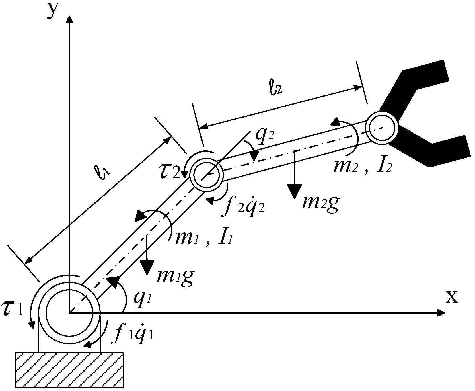
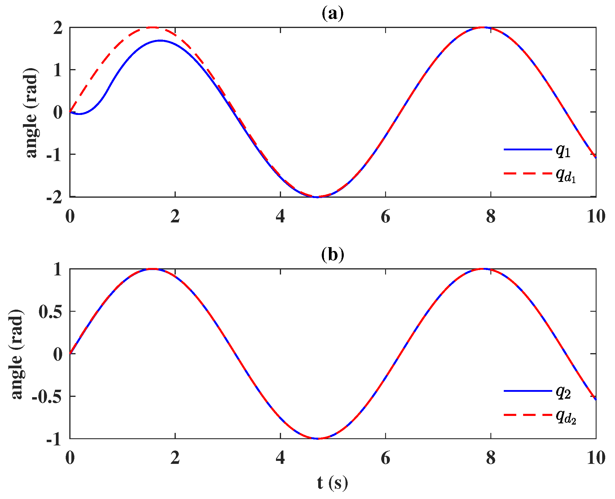
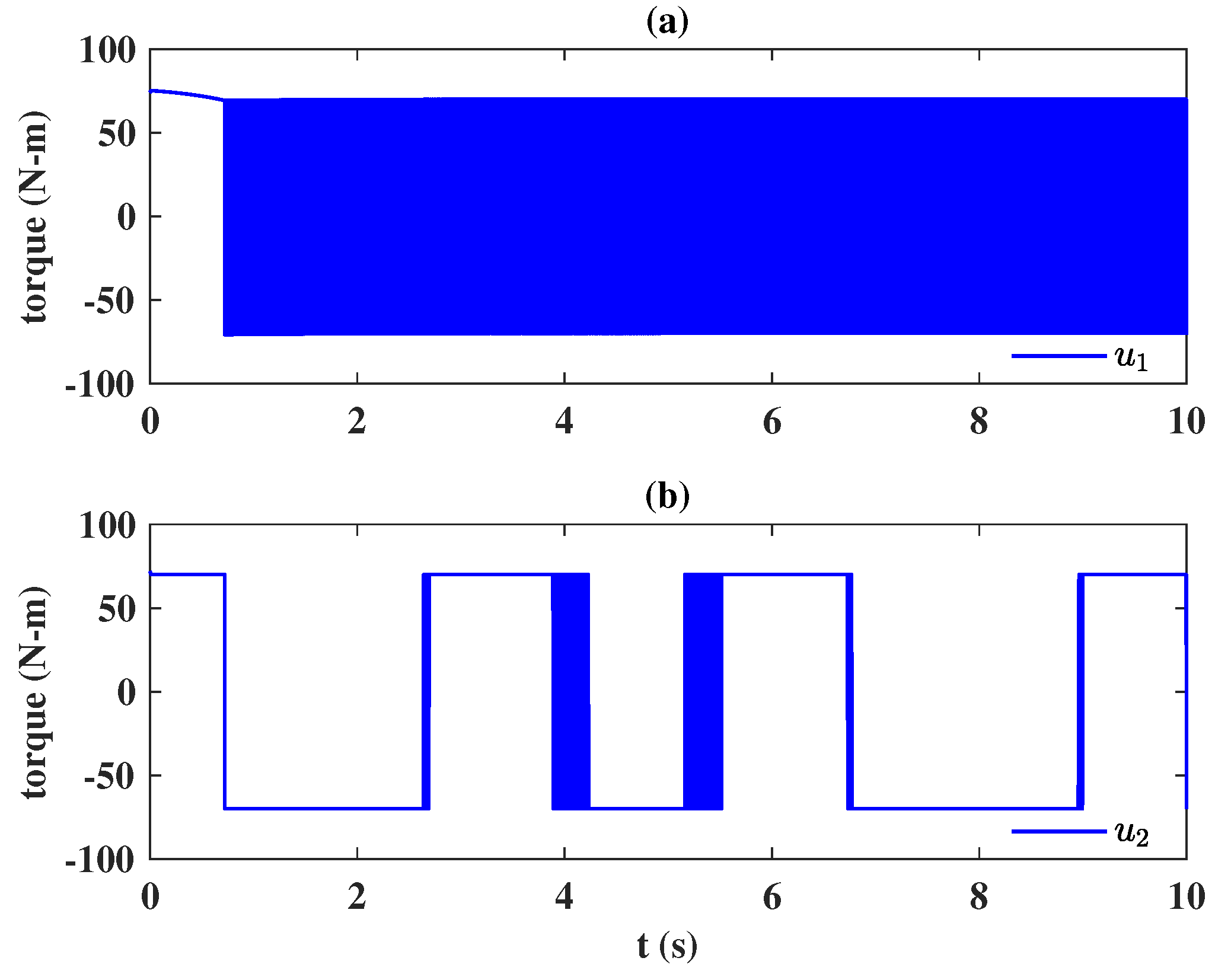
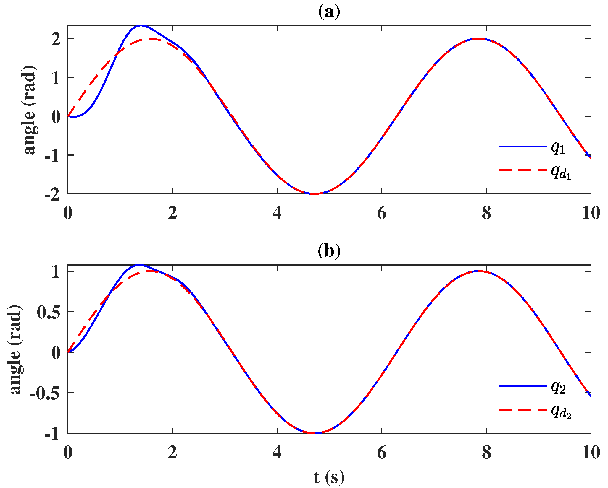
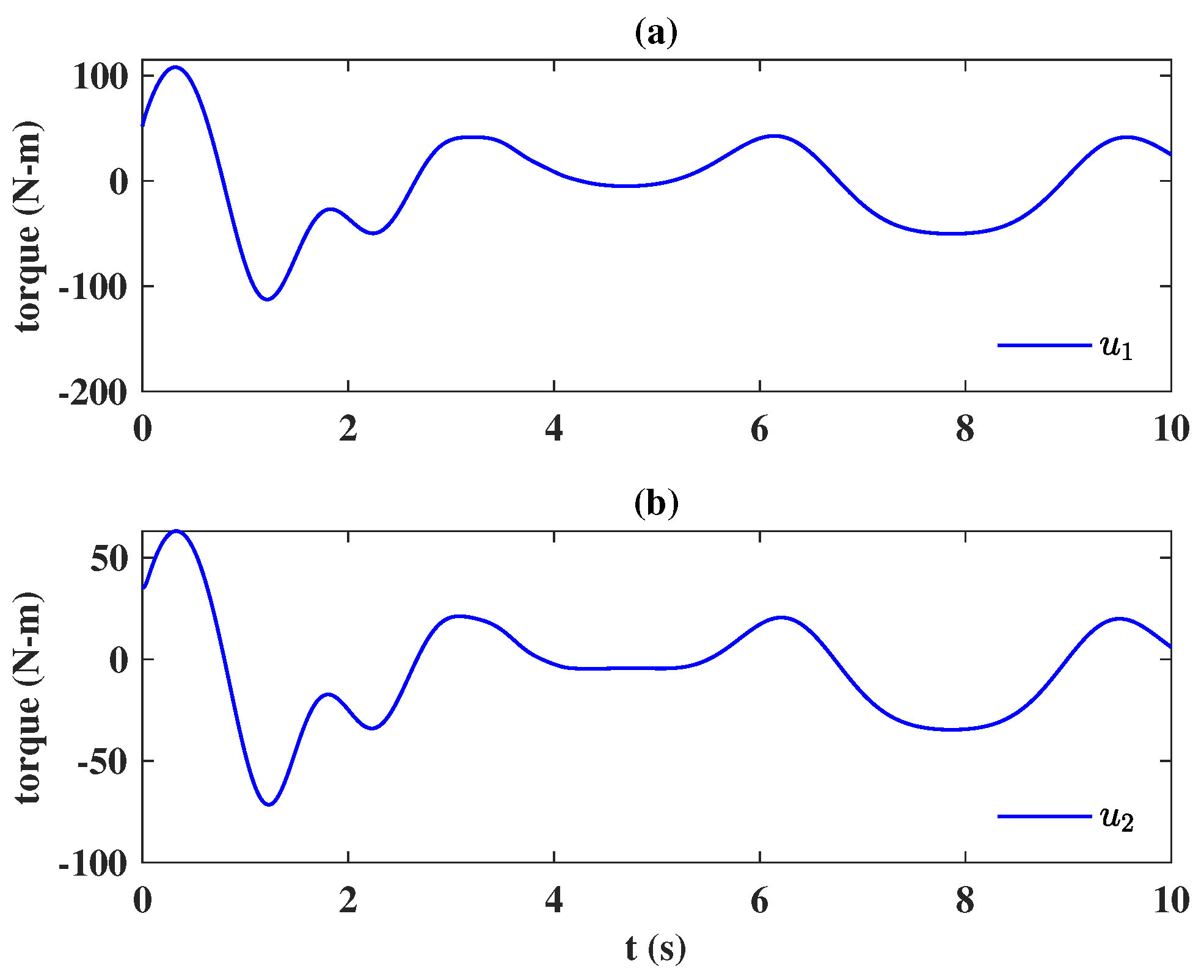
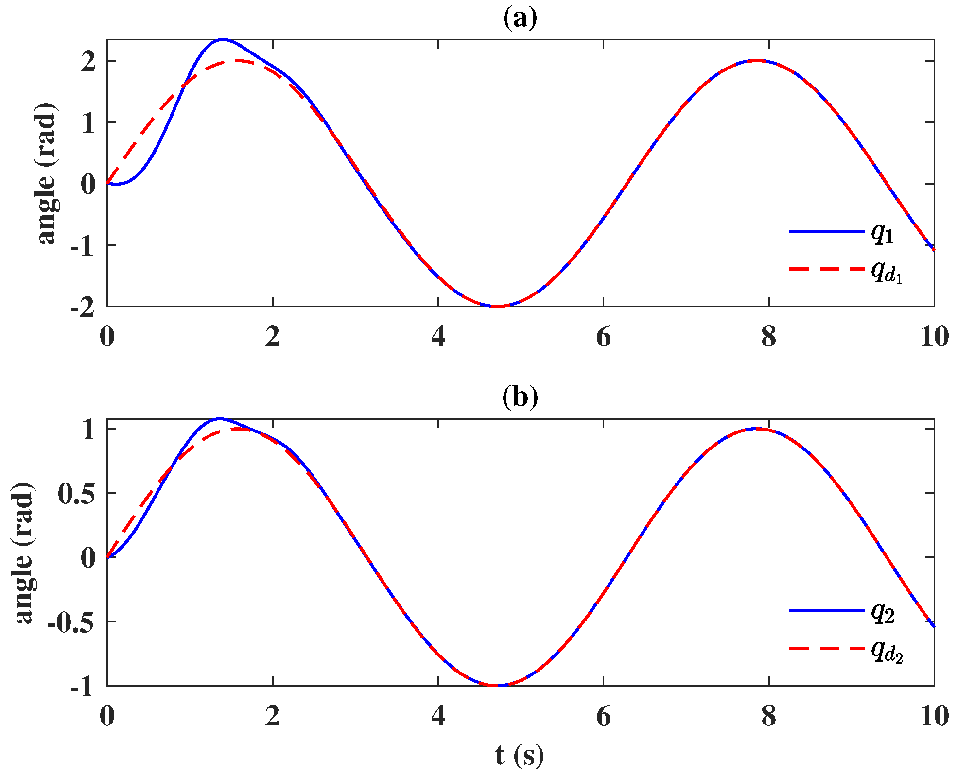
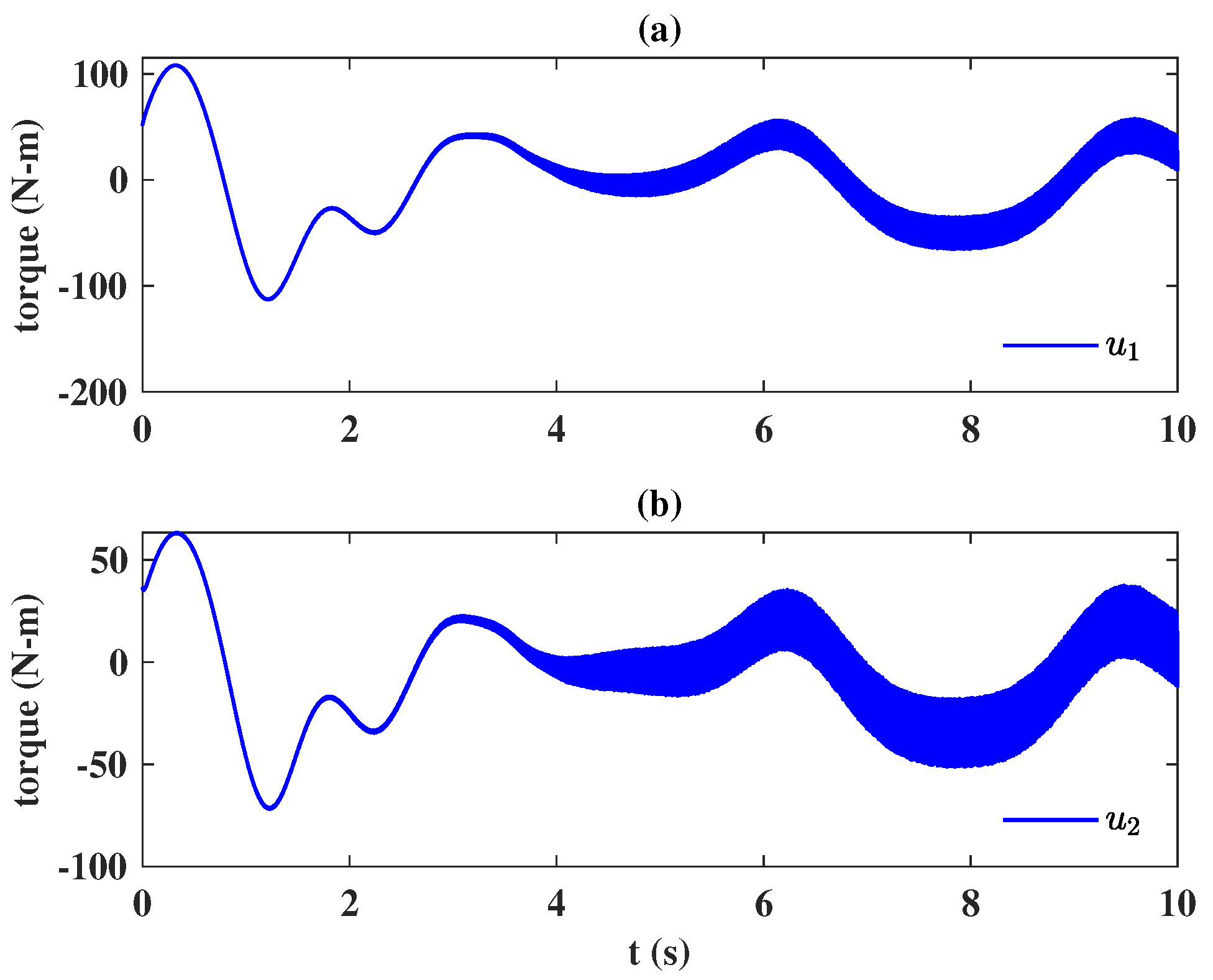
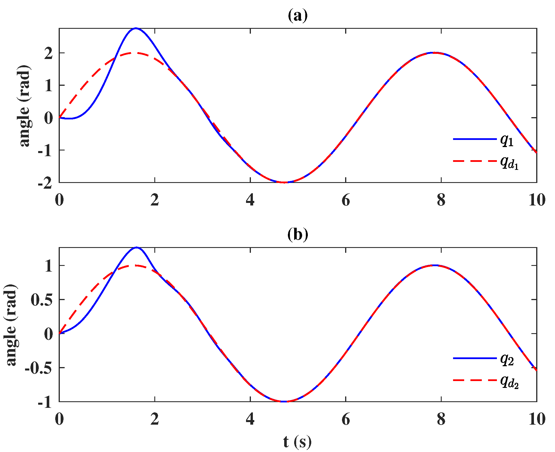
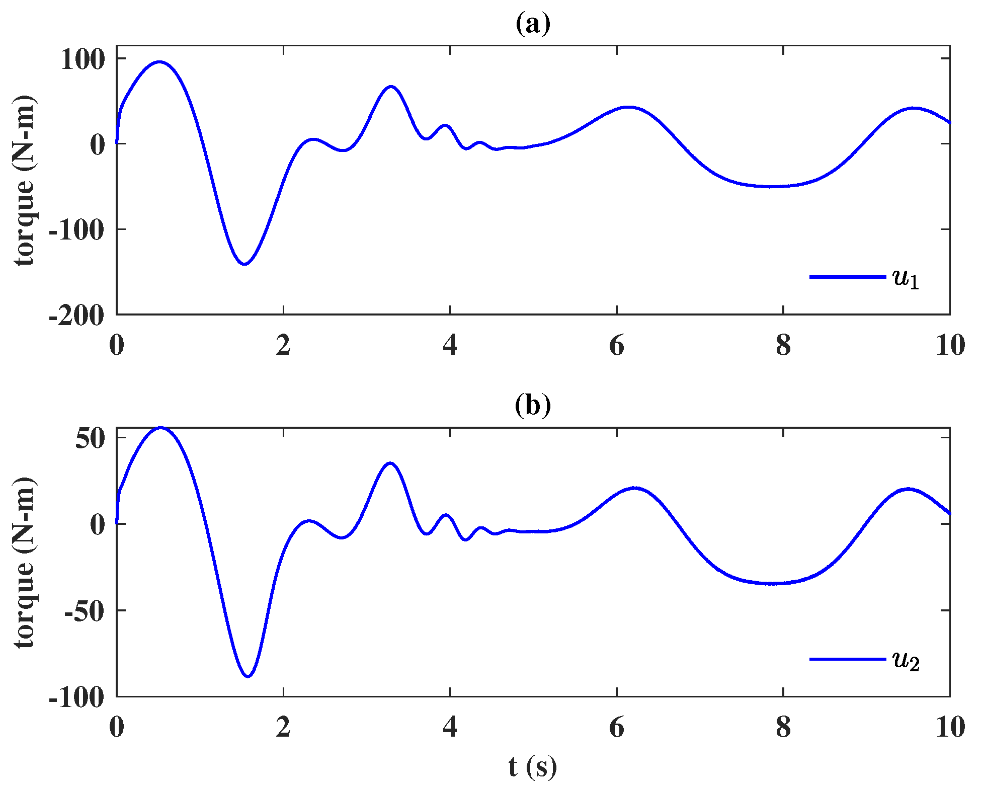
6. Application to a Two DOF Robot Manipulator

A two-link robot studied by [9] is used here to illustrate the efficiency of the proposed control design. As shown in Figure 3, the manipulator is in the vertical position, and the parameters are shown in

Table 1. System parameters of the two-link robot.

Parameters	Value
$l_1$	1  m
$l_2$	2  m
$m_1$	1  kg
$m_2$	1  kg
$l_{c1}$	1  m
$l_{c2}$	2  m
$f_1$	$0.3\mathrm{N}·\mathrm{m}·\mathrm{s}/\mathrm{rad}$
$f_2$	$0.3\mathrm{N}·\mathrm{m}·\mathrm{s}/\mathrm{rad}$

. System matrices in (1) are defined as in [9]:

$$\begin{array}{cc}\hfill M& =\left[\begin{array}{cc}{m}_1{l}_{c1}^2+m_2(l_1^2+l_{c2}^{2}cos(q_2))+I_1+I_2& m_2(l_{c2}^2+l_2{l}_{c2}cos(q_2))+I_2\\ m_2(l_{c2}^2+I_1{I}_{c2}cos(q_2))+I_2& m_2{l}_{c2}^2+I_2\end{array}\right]\hfill \\ \hfill C& =\left[\begin{array}{cc}-2m_2{l}_1{l}_{c2}sin(q_2){\dot{q}}_2& -m_2{l}_1{l}_{c2}sin(q_2){\dot{q}}_2\\ m_2{l}_1{l}_{c2}sin(q_2){\dot{q}}_2& 0\end{array}\right]\hfill \\ \hfill G& =\left[\begin{array}{c}{m}_{2}gcos(q_1+q_2)+(m_1+m_2)g{l}_{1}cos(q_1)\\ m_{2}g{l}_{2}cos(q_1+q_2)\end{array}\right],F=\left[\begin{array}{cc}{f}_1& 0\\ 0& f_2\end{array}\right],\hfill \end{array}$$

(53)

and the desired trajectories are

$$\begin{array}{c}\hfill q_d=\left[\begin{array}{c}2sin(t)\\ sin(t)\end{array}\right].\end{array}$$

(54)

In this case, the system matrices (53) are assumed to be unknown and considered as system uncertainties and disturbances in (5), and the system matrices in the closed-loop system (5) are

$$\begin{array}{c}\hfill A=\left[\begin{array}{cccc}0& 1& 0& 0\\ 0& 0& 0& 0\\ 0& 0& 0& 1\\ 0& 0& 0& 0\end{array}\right],B=\left[\begin{array}{cc}0& 0\\ 1& 0\\ 0& 0\\ 0& 1\end{array}\right].\end{array}$$

(55)

Conventionally, the sliding-mode control design [17] for the uncertain system (5) is constructed as

$$\begin{array}{c}\hfill u=-Kx-\xi \frac{s}{\parallel s\parallel },\end{array}$$

(56)

where

$$\begin{array}{c}\hfill K=\left[\begin{array}{cccc}1& 2& 0& 0\\ 0& 0& 1& 2\end{array}\right]\end{array}$$

is the state feedback gain that places eigenvalues of $A-BK$ in the open left-half plane. As the nominal closed-loop system matrix $A_c=A-BK$ is stable, a positive definite matrix P exists, satisfying the Lyapunov equation [35]

$$\begin{array}{c}\hfill A_c^{T}P+P{A}_c=-I.\end{array}$$

(57)

In the control law (56), s is the sliding variable

$$\begin{array}{c}\hfill s=2B^{T}Px,\end{array}$$

(58)

where P is obtained from the Lyapunov equation (57) and the constant $\xi =70$ is an upper bound of unknown disturbances. Figure 4 shows that the system outputs track desired references when the time exceeds 4 s with the sliding-mode control design, and Figure 5 shows the time history of the control signals. It can be seen that the control inputs suffer from the chattering phenomenon because the discontinuous switching function $\mathrm{sgn}(·)$ is used in the control design (56). By contrast, the robust linear control design (11) is employed to deal with the uncertain system (5), where K is the state feedback gain that places the eigenvalue of $A_c$ in (12) to $[-\rho ,-2\rho ,-3\rho ,-4\rho ]$, and the design parameter $\rho >0$ observes the scheduling law

$$\begin{array}{c}\hfill \rho (t)=\frac{\overline{\rho }}{2}(\frac{t-T}{|t-T|+ϵ}+1),\end{array}$$

(59)

where $\overline{\rho }=50$, $T=4$ and $ϵ=1$ to provide a similar convergent speed as the sliding-mode control design (56). In Figure 6, the tracking performance with the robust linear control (11) is depicted, and Figure 7 presents the control signals. It is seen the robust linear control (11) performs the robustness as the sliding-mode control design (56) with a much more straightforward design algorithm; moreover, the chattering phenomenon in Figure 5 is absent, and the undesirable peaking phenomenon [17] is eliminated.

When a uniform distributed measurement noise in the interval $[-0.001,0.001]$ is added to the state measurement of x, the control performance of proposed robust linear control is shown in Figure 8 and Figure 9. Figure 8 shows that the control mission is achieved even if the measurement is corrupted by a stochastic noise. However, as depicted in Figure 9, when the design parameter $\rho$ in (59) is increasing, the interference of measurement noise is increased in the control signals; as discussed in Remark 4, the control signal is coupled with an undesirable, high-frequency oscillation when the state feedback gain K is correspondingly large.

Because the measurement process always couples with measurement noise, the undesirable oscillation occurs when the control design (11) is implemented. Therefore, developing the robust noise-free control design is necessary for eliminating the noise-induced chattering. As an intuitive augmentation of (11), the state feedback gain K of the robust noise-free control in (33) is designed to place the poles of system (52) to $[-\rho ,-2\rho ,-3\rho ,-4\rho ,-5\rho ,-6\rho ]$, and the design parameter $\rho$ are scheduled as in (59). The controlled system response is depicted in Figure 10. Following the same concept of pole placement, the exponent ${\sigma }_0$ in (41) coincides with $\sigma$ in (28); the convergent speed of robust linear control (30) and robust noise-free linear control (45) are dominated by the same singular value when $\rho$ is large (Figure 11). On the other hand, because of the high-frequency oscillation is filtered out by the integrator, the control inputs of the noise-free design are smooth even if the state measurement is corrupted by a stochastic noise and the control gain K is scheduled to a high level; moreover, the peaking phenomenon [17] which often occurs in high-gain control is absent due to the design control structure and the scheduling law (59).

7. Conclusions

This paper shows that simple linear control can effectively suppress large system uncertainties and external disturbances. The proposed linear control is simple, has no side effect of control chattering even in a noisy environment, and can deal with large system uncertainties and large external disturbances as effectively as the sliding mode control does. In the application example, the noise-free design is implemented in a robot manipulator. The simulation results confirm that the proposed robust noise-free control algorithm is an intuitive design that requires minimum computational effort, and therefore can be easily accepted by control engineers with only fundamental control knowledge, and the actuators in real world are protected.

References

1. Lewis, F.L.; Dawson, D.M.; Abdallah, C.T. Robot Manipulator Control: Theory and Practice; CRC Press: Boca Raton, FL, USA, 2003. [Google Scholar]
2. Callier, F.M.; Desoer, C.A. Linear System Theory; Springer Science & Business Media: Boston, NY, USA, 2012; Chapter 7.2. [Google Scholar]
3. Slotine, J.J.E.; Li, W. On the adaptive control of robot manipulators. Int. J. Robot. Res. 1987, 6, 49–59. [Google Scholar] [CrossRef]
4. Zhang, D.; Wei, B. Adaptive Control for Robotic Manipulators; CRC Press: Boca Raton, FL, USA, 2017. [Google Scholar]
5. Jin, M.; Lee, J.; Tsagarakis, N.G. Model-free robust adaptive control of humanoid robots with flexible joints. IEEE Trans. Ind. Electron. 2016, 64, 1706–1715. [Google Scholar] [CrossRef]
6. Slotine, J.J.; Sastry, S.S. Tracking control of non-linear systems using sliding surfaces, with application to robot manipulators. Int. J. Control 1983, 38, 465–492. [Google Scholar] [CrossRef] [Green Version]
7. Doulgeri, Z. Sliding regime of a nonlinear robust controller for robot manipulators. IEE Proc. Control Theory Appl. 1999, 146, 493–498. [Google Scholar] [CrossRef]
8. Fu, L.C.; Liao, T.L. Systems Using Variable Structure Control and with an Application to a Robotic. IEEE Trans. Autom. Control 1990, 35, 1345–1350. [Google Scholar] [CrossRef]
9. Lin, C.J. Variable structure model following control of robot manipulators with high-gain observer. JSME Int. J. Ser. Mech. Syst. Mach. Elem. Manuf. 2004, 47, 591–601. [Google Scholar] [CrossRef]
10. Islam, S.; Liu, X.P. Robust sliding mode control for robot manipulators. IEEE Trans. Ind. Electron. 2010, 58, 2444–2453. [Google Scholar] [CrossRef]
11. Navvabi, H.; Markazi, A.H. New AFSMC method for nonlinear system with state-dependent uncertainty: Application to hexapod robot position control. J. Intell. Robot. Syst. 2019, 95, 61–75. [Google Scholar] [CrossRef]
12. He, W.; Dong, Y.; Sun, C. Adaptive neural impedance control of a robotic manipulator with input saturation. IEEE Trans. Syst. Man Cybern. Syst. 2015, 46, 334–344. [Google Scholar] [CrossRef]
13. Jin, L.; Li, S.; Yu, J.; He, J. Robot manipulator control using neural networks: A survey. Neurocomputing 2018, 285, 23–34. [Google Scholar] [CrossRef]
14. Elsisi, M.; Mahmoud, K.; Lehtonen, M.; Darwish, M.M. An improved neural network algorithm to efficiently track various trajectories of robot manipulator arms. IEEE Access 2021, 9, 11911–11920. [Google Scholar] [CrossRef]
15. Utkin, V. Variable structure systems with sliding modes. IEEE Trans. Autom. Control 1977, 22, 212–222. [Google Scholar] [CrossRef]
16. Hung, J.Y.; Gao, W.; Hung, J.C. Variable structure control: A survey. IEEE Trans. Ind. Electron. 1993, 40, 2–22. [Google Scholar] [CrossRef] [Green Version]
17. Khalil, H.K. Nonlinear Systems; Prentice-Hall: Upper Saddle River, NJ, USA, 2002; Chapter 14. [Google Scholar]
18. Fridman, L.M. An averaging approach to chattering. IEEE Trans. Autom. Control 2001, 46, 1260–1265. [Google Scholar] [CrossRef]
19. Boiko, I. Discontinuous Control Systems: Frequency-Domain Analysis and Design; Springer Science & Business Media: Boston, NY, USA, 2008. [Google Scholar]
20. Burton, J.; Zinober, A.S. Continuous approximation of variable structure control. Int. J. Syst. Sci. 1986, 17, 875–885. [Google Scholar] [CrossRef]
21. Levant, A. Higher-order sliding modes, differentiation, and output-feedback control. Int. J. Control 2003, 76, 924–941. [Google Scholar] [CrossRef]
22. Tayebi-Haghighi, S.; Piltan, F.; Kim, J.M. Robust composite high-order super-twisting sliding mode control of robot manipulators. Robotics 2018, 7, 13. [Google Scholar] [CrossRef] [Green Version]
23. Ahmed, S.; Wang, H.; Tian, Y. Adaptive high-order terminal sliding mode control based on time delay estimation for the robotic manipulators with backlash hysteresis. IEEE Trans. Syst. Man Cybern. Syst. 2019, 51, 1128–1137. [Google Scholar] [CrossRef]
24. Ahmed, S.; Wang, H.; Tian, Y. Adaptive Fractional High-order Terminal Sliding Mode Control for Nonlinear Robotic Manipulator under Alternating Loads. Asian J. Control 2020. [Google Scholar] [CrossRef]
25. Brahmi, B.; Driscoll, M.; Laraki, M.H.; Brahmi, A. Adaptive high-order sliding mode control based on quasi-time delay estimation for uncertain robot manipulator. Control Theory Technol. 2020, 18, 279–292. [Google Scholar] [CrossRef]
26. Yeh, Y.L.; Chen, M.S. Frequency domain analysis of noise-induced control chattering in sliding mode controls. Int. J. Robust Nonlinear Control 2011, 21, 1975–1980. [Google Scholar] [CrossRef]
27. Oliveira, T.R.; Estrada, A.; Fridman, L.M. Global and exact HOSM differentiator with dynamic gains for output-feedback sliding mode control. Automatica 2017, 81, 156–163. [Google Scholar] [CrossRef]
28. Chen, B.S.; Wong, C.C. Robust linear controller design: Time domain approach. IEEE Trans. Autom. Control 1987, 32, 161–164. [Google Scholar] [CrossRef]
29. Sobel, K.M.; Bandaj, S.S.; Yeh, H.H. Robust control for linear systems with structured state space uncertainty. Int. J. Control 1989, 50, 1991–2004. [Google Scholar] [CrossRef]
30. Siciliano, B.; Sciavicco, L.; Villani, L.; Oriolo, G. Robotics: Modelling, Planning and Control; Springer Science & Business Media: Boston, NY, USA, 2010; Chapter 9.3. [Google Scholar]
31. Draženović, B. The invariance conditions in variable structure systems. Automatica 1969, 5, 287–295. [Google Scholar] [CrossRef]
32. Bronson, R.; Saccoman, J.T.; Costa, G.B. Linear Algebra: Algorithms, Applications, and Techniques; Academic Press: Cambridge, MA, USA, 2013; Chapter 4.3. [Google Scholar]
33. Chen, C.T. Linear System Theory and Design; Holt, Rinehart and Winston: New York, NY, USA, 1984; Chapter 4.4. [Google Scholar]
34. Chen, M.S.; Chen, C.H.; Yang, F.Y. An LTR-observer-based dynamic sliding mode control for chattering reduction. Automatica 2007, 43, 1111–1116. [Google Scholar] [CrossRef]
35. Vidyasagar, M. Nonlinear Systems Analysis; Prentice-Hall: Englewood Cliffs, NJ, USA, 1993; Chapter 5.4. [Google Scholar]
Figure 1. σ B N ( σ ) versus σ .
Actuators 10 00121 g001
Figure 2. Block structure of noise-free control.
Actuators 10 00121 g002
Figure 3. The schematic diagram of two-DOF manipulator.
Actuators 10 00121 g003
Figure 4. Time history of system outputs and references: (a) q 1 and q d 1 , (b) q 2 and q d 2 (sliding-mode control).
Actuators 10 00121 g004
Figure 5. Time history of control signals: (a) u 1 and (b) u 2 (sliding-mode control).
Actuators 10 00121 g005
Figure 6. Time history of system outputs and references: (a) q 1 and q d 1 , (b) q 2 and q d 2 (robust linear control).
Actuators 10 00121 g006
Figure 7. Time history of control signals: (a) u 1 and (b) u 2 (robust linear control).
Actuators 10 00121 g007
Figure 8. Time history of system outputs and references: (a) q 1 and q d 1 , (b) q 2 and q d 2 (robust linear control with noise).
Actuators 10 00121 g008
Figure 9. Time history of control signals: (a) u 1 and (b) u 2 (robust linear control with noise).
Actuators 10 00121 g009
Figure 10. Time history of system outputs and references: (a) q 1 and q d 1 , (b) q 2 and q d 2 (robust noise-free linear control).
Actuators 10 00121 g010
Figure 11. Time history of control signals: (a) u 1 and (b) u 2 (robust noise-free linear control).
Actuators 10 00121 g011