1. Introduction
In recent years, household consumption of energy has drastically increased due to the rapid growth rate observed in the world’s population. With the increase in population, houses have also expanded, and the use of appliances has become more common. Household appliances such as air conditioners, heaters, refrigerators, washing machines, stoves, etc., all operate on energy. Early prediction of a household’s energy usage can help in better managing of the energy needs and planning to save energy where possible. Hence, predicting electricity demand is crucial, as it plays a pivotal role in utility power planning [
1]. Effective and accurate energy consumption models cannot be overemphasized and are one of the major challenges [
2,
3].
A context-aware energy prediction mechanism is one where roles of all the sensing values from the environment surroundings are carefully observed. For example, in a smart home’s energy consumption prediction problem, the context can include the smart home appliances’ power consumption, weather conditions, users’ activities, time of the day, day of the week, workday or holiday, special events, etc. A prediction mechanism must consider the surroundings of the given environment and the fact that the surrounding relevance is also variable. Another major concern while implementing a prediction model is selecting the most appropriate features.
Feature selection is one of the most important steps in prediction problems. The process of feature selection can be defined as finding the smallest subset that shows the strongest effect on the prediction accuracy and minimizes the model’s complexity. Finding the most related input features is essential. To select the right features, one must have detailed and in-depth knowledge of the area. Still, manual feature selection is a very tedious task, and even experts in a field can make mistakes. The accuracy of the prediction model greatly depends on the quality of data and the relevancy of features. For example, in case of energy prediction, if the given features in a dataset have no strong relation to the increase or decrease in the energy consumption, then there are high chances that the model performance will turn out to be poor. A prediction model, which is enabled to learn feature importance on its own, with the passage of time, can be of huge benefit to prediction problem applications.
In this work, we focused on the use of a long short-term memory (LSTM) algorithm in prediction models. LSTM is a type of recurrent neural network (RNN). It is a time-series forecasting algorithm [
4]. LSTM networks are considered one of the most suitable prediction algorithms for time series data. In recent years, many researchers have focused on proposing prediction algorithms using the efficacy of LSTMs. Xiangyun et al. propose an hourly day-ahead solar irradiance prediction algorithm, using LSTMs, for minimizing energy costs [
5]. An energy consumption prediction mechanism for smart homes based on a hybrid LSTM network is proposed by Ke et al. [
6]. The hybrid approach increases the data dimensions and eventually results in increased prediction accuracy.
In this work, we present a predictive learning-based optimal actual control mechanism for smart homes. The proposed mechanism includes a prediction learning module that uses LSTM to make energy consumption predictions. The prediction module takes all available features at the first cycle of learning and works its way down to learn the most impactful features. The prediction model also learns to re-add features based on the relevance of history learned at a given prediction time. The predicted values are then passed onto the optimization module, where optimal parameters are set accordingly. Optimal parameters are then used to generate actuator control commands.
The rest of the paper is divided as follows:
Section 2 presents the related works;
Section 3 presents the proposed prediction mechanism. In
Section 4, we provide the task modeling simulation of the proposed system. Results analysis is presented in
Section 5;
Section 7 concludes the paper with discussions.
2. Related Work
Energy consumption prediction is one of the significant prediction problems, and many recent researchers have proposed solutions for energy prediction based on deep learning, such as load forecast-based on pinball loss guided LSTM [
7], energy use prediction for solar-assisted water heating system [
8], and short-term residential load forecasting using LSTM recurrent neural network [
9,
10]. An LSTM-based periodicity energy usage of a cooling system is analyzed in [
11]. According to this study, the computation cost can be reduced by using lower dimensional variables. A hybrid LSTM-based approach that integrated data pretreatment strategy, deep learning method, and advanced optimization method, is introduced in [
12]. It is referred as a short-term energy load forecast system known as VMD-BEGA-LSTM (VLG), integrating a data pretreatment strategy, advanced optimization technique, and deep learning structure, is developed in this paper.
LSTMs have been widely used in contextual recommendation systems. A context-aware location recommendation system is proposed by Wafa et al. The authors propose a hierarchical LSTM model. The two-level hierarchy model predicts the location of interest at the first level and considers the contextual information related to predicted location at the second level [
13].
Yirui et al. propose a context-aware attention LSTM network model for flood prediction. The authors focus on predicting sequential flow rates based on flood factors. Their proposal aims to remove the irrelevant flood factors data to avoid noise and emphasize on the informative factors only. Their proposed model learns the probability distributions between flow rate and hidden output of each LSTM during training and assigns the weights accordingly during testing [
14]. The installment of IoT sensors in smart building enables action recognition and hence, it leads to real-time monitoring, control, and savings of energy. A context-aware load supply mechanism based on IoT and deep learning is presented. The context-aware network is built on classroom video and action recognition data is extracted to extract contexts [
15]. Joshua et al. present a hot water energy demand prediction for saving energy using convolutional neural networks (CNNs). They make the use of contextual data such hour, day, week, etc., to extract contextual information [
16].
Jeong et al. present a context-aware LSTM for event time series prediction. Their proposed model is based on hidden Markov model (HMM) and LSTM. HMM is used to abstract the past data for distant information of context [
17]. Maria et al. make an effort to cover two properties of non-intrusive load monitoring, non-causality and adaptivity to contextual factors, via application of bidirectional LSTM model. The authors develop a self-training-based adaptive mechanism to address scaling issues with the increase in smart home appliances [
18]. Another scalable and non-intrusive load monitoring approach is presented by Kunjin et al. A convolutional neural network (CNN)-based model is proposed for building a multi-branch architecture, with an aim to improve prediction accuracies [
19]. Tae et al. present a CNN-LSTM-based hybrid mechanism for household power consumption prediction [
20]. Yan et al. present a CNN-LSTM-based integrated energy prediction approach for Chinese energy structure. In order to verify the results, the authors compared their proposal results with six methods such as ARIMA, KGM, SVM, PBNN, LSTM, and CNN [
21]. Many recent works have proposed hybrid of popular prediction algorithms to present a more robust solution [
22,
23,
24,
25,
26].
Many recent studies have focused on the context-aware load prediction solutions. The existing solution of context-aware predictions can be widely categorized into two types: context feature extraction in pre-processing and context features weights assignment during learning. Based on our related works’ study, we observed that a major difference in the prediction results might occur; if past predictions’ context is recorded, and feature learning is performed before weighing the features during training process. A summary of context-aware prediction solutions is presented in
Table 1.
Feature learning and selection based on feature importance is also very crucial when it comes to learning contexts and updating model accordingly. In [
27], an integrated feature learning technique is proposed for predicting travel time by using deep learning. To increase the learnability of features, different feature enriching algorithms are applied. In [
28], the focus is on selecting effective features through a strategy that minimizes the redundancy and maximizes the relevancy of features. The study analyzes the influence of selecting effective features on load consumption of building. In another study [
29], deep learning and Bat algorithms are used for optimizing energy consumption and for user preference-based feature selection. A hybrid approach [
30] that is integrated with feature selection method aims to automatically detect the features based on higher relevance for multi-step prediction. In [
31], two main tasks are performed: first, a method is proposed to transform the time-dependent data for machine learning algorithms and secondly, different kind of feature selection tasks are applied for regression tasks.
A similar sort of model is presented in [
32], that is developed by using layered structures and meta-features. In [
33], a neuro-fuzzy inference system is proposed that is being boosted with an optimizer. It also introduced a new non-working time adaptation layer. In [
34], an LSTM-based model with various configurations is built to forecast energy consumption. It uses wrapper and embedded feature selection techniques along with genetic algorithm (GA) to find optimal configuration of LSTM for prediction learning.
Prediction learning models are updated periodically, due to updates in history data. Hence, it is wise to record additional results from previous test results and use the data to benefit the system in next training cycles. In this work, we propose a feature learning solution that aims to improve the prediction accuracies by filtering the contextual data based on history learnings.
3. Proposed Prediction Mechanism
This section presents a feature learning-based adaptive LSTM approach for energy predictions in smart environments. Our proposed prediction model takes all available features at the first cycle and works its way down to learn the most impactful features. The proposed model also learns to re-add features based on relevance with a change in attributes involved and time. Hence, we can call the proposed model to be adaptive in nature.
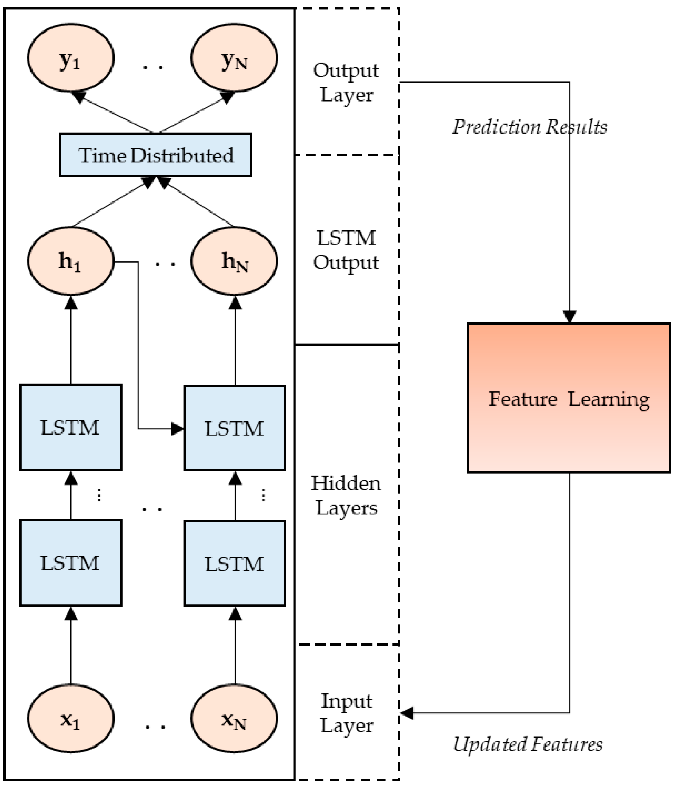
In
Figure 1, we present the proposed prediction model, where an LSTM algorithm is used for making predictions. The proposed model has a feature learning module integrated with LSTM predictions in a cyclic manner. After every cycle of LSTM prediction, the outputs are passed onto the feature learning module, where features are tuned, and then updated features are passed onto the next cycle of predictions.
3.1. LSTM Architecture
LSTM is a type of RNN (recurrent neural network) where prediction is performed by backpropagation. The output of a neural network layer is backpropagated at time “t” to the input of the same network layer at time ‘t + 1’.
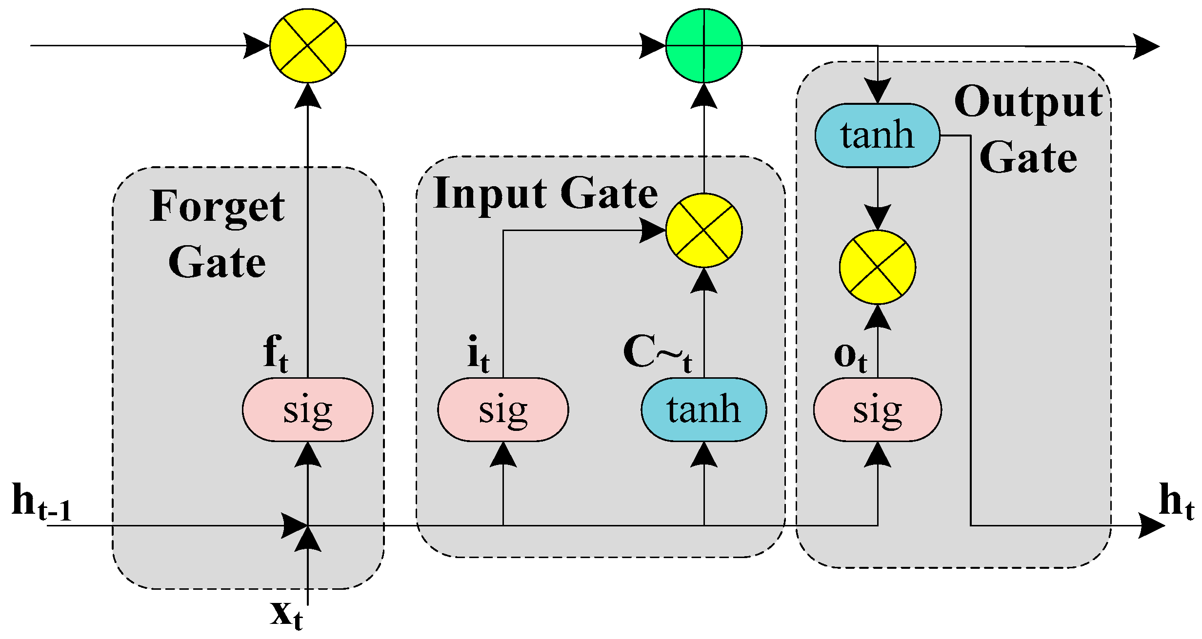
LSTM contains memory blocks that are connected through layers. A block contains three gates that enable the block to maintain its states and output. The three gates included in an LSTM block are a forget gate, an input gate, and an output gate. The forget gate conditionally decides which information can be ignored and which information is important to be remembered. The input gate decides what values from input should be used to update the state. The output gate decides what should be the output based on the block’s current input and state memory.
In equations flow below, we present the operations performed at forget gate, input gate, and output gate. The terms used are described in
Table 2.
Equation (1) shows the operation of forget gate which decides what elements of the previous cell state (
Ct−1) are to be forgotten.
Next, Equation (2) shows that which values is to be updated at input gate.
Then a potential vector of cell state is computed by the current input (
) and the last hidden state
.
After that, we can update the old cell state
into the new cell state
by element-wise multiplication as shown in Equation (4) below.
The output gate decides which elements to output by a sigmoid layer (Equation (5)).
The new hidden state
of LSTM is then calculated by combining Equations (4) and (5).
In
Figure 2 below, we show the block structure of LSTM including forget gate, input gate, and output gate.
3.2. Feature Learning
In this subsection, we present the feature learning method. The training and testing process using the LSTM algorithm is performed in cycles.
All features’ relevance data is added to feature relevance history data. This history data is built by reiterating training and testing cycles, with feature deductions, shuffling, and reset. The aim of maintaining history log for feature relevance score is to make the system capable of learning from features relevance context based on time of predictions. The feature history data is updated with each cycle by adding prediction results attributes such as time of the day, day of the week, workday/holiday, and all features relevance score.
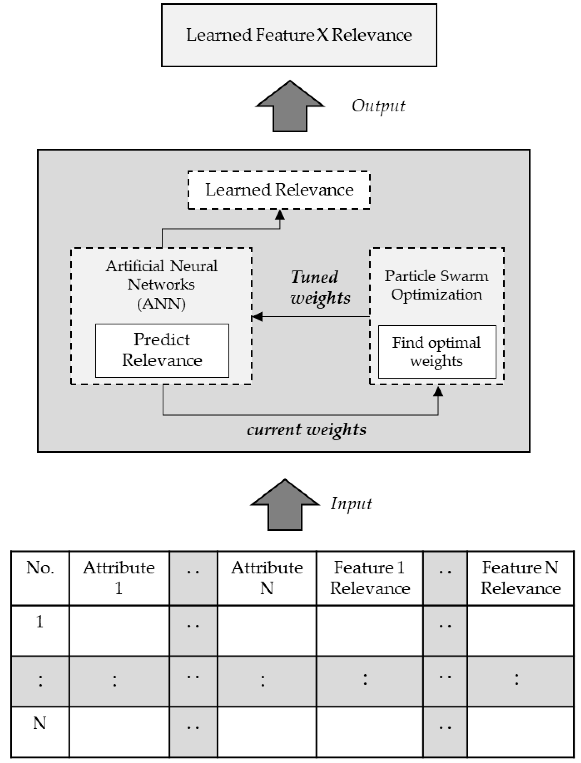
We have used an artificial neural network (ANN) algorithm for learning feature relevance, and we have used PSO algorithm to optimize the weights. PSO takes weights from ANN at each iteration, and PSO populations work towards finding optimal weights. The tuned weights are passed back to ANN. The optimization of ANN weights with PSO aims to reduce learning time and improve learning rates (
Figure 3).
3.3. Meta-Parameters
This section presents some meta-parameters used during various processes and methods, such as different thresholds. These meta-parameters are set after multiple experiments, and the most optimal values are used. Other meta-parameters include total processing capacity, layers in ANN, PSO’s inertia velocity boost threshold, and PSO’s regeneration threshold. These thresholds are also used to examine the particle’s performance in PSO.
Table 3 presents the optimal values of different meta-parameters after multiple experiments, as shown in [
35]. In different applications, users may have to tinker with these values to fine-tune their results.
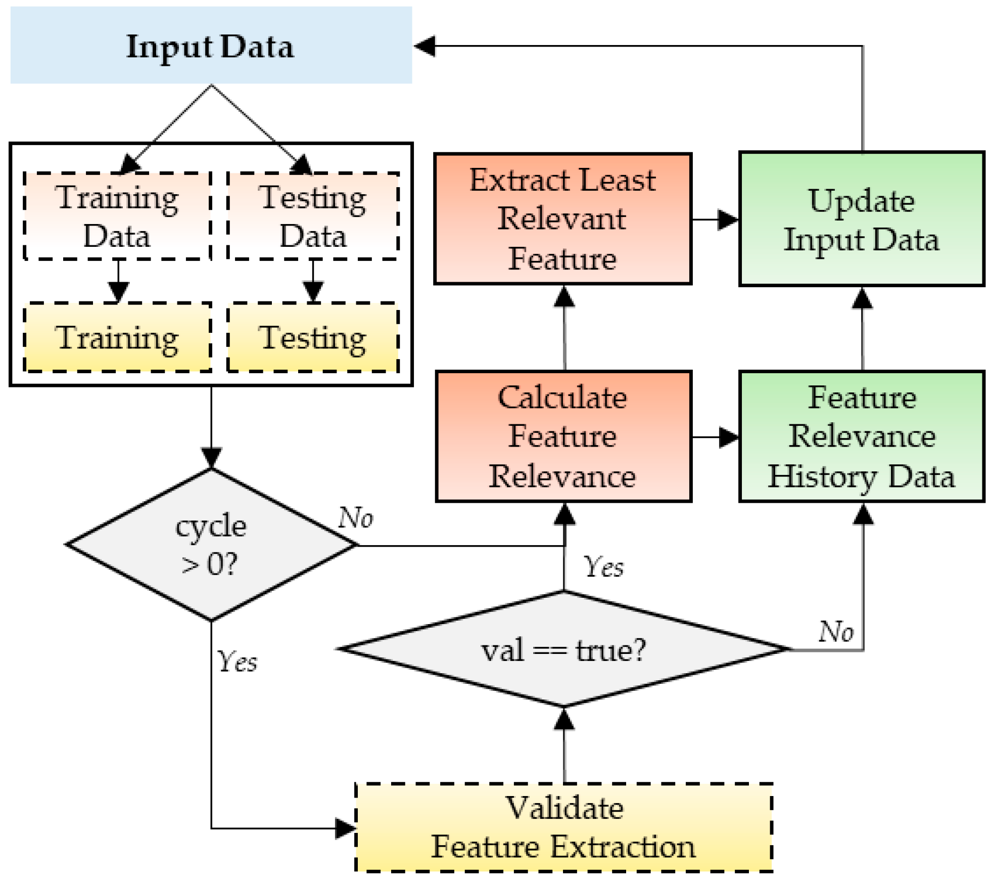
After the first cycle of LSTM training and testing, each feature’s prediction scores, and relevance score are extracted. A relevance threshold is set, and a relevance score below the threshold is considered unacceptable. After the first cycle, the least relevant feature is removed, and the next cycle of prediction is performed with updated input data. From the second iterations onwards, the system first validates the prediction performance after removal of the last least relevant feature. If prediction performance is improved or no change is observed, then validation is set to true. Otherwise, if prediction performance deteriorates after feature removal, then validation is set to false. When validation is true, the relevance score for all existing features is extracted, and the feature with the least relevance is removed. When validation is false, the last removed feature is added back, and a positive weight is added to its relevance history data (
Figure 4).
After the removal or addition of features based on validation results, the history data learning results are extracted. Features with high relevance score based on learnings from history data are matched to be present in the data, and features with relevance below than a set threshold are removed.
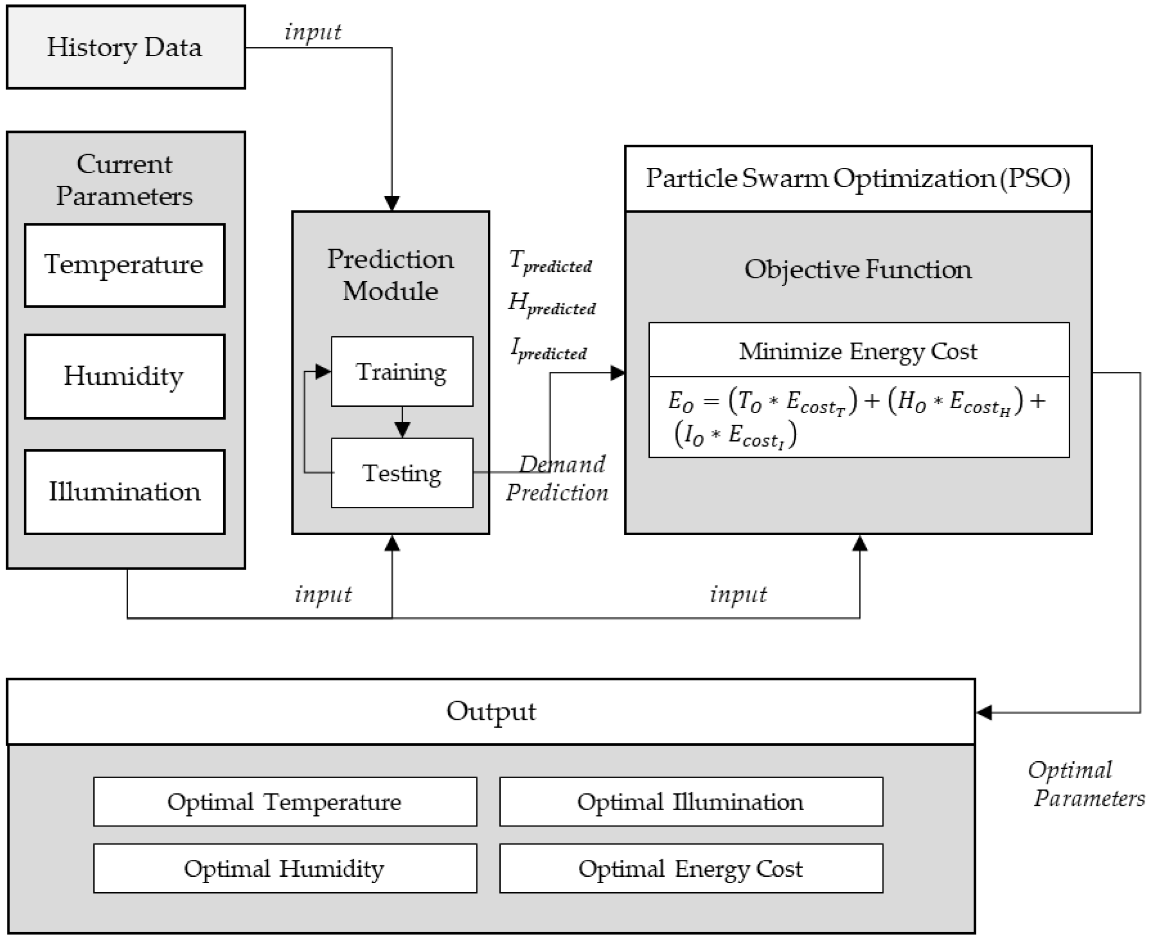
3.4. Predictive Learning-Based Optimal Control Mechanism
In this section, we present the predictive learning-based control mechanism for smart home actuators’ control commands generation and scheduling the control commands. We upgrade the optimal control scheduling mechanisms from one of our recently published works [
36] and transform it into a predictive learning-based optimal control mechanism to improve the architecture design and performance. In [
36], we defined the optimization objective function based on user-defined parameters. In this proposal, the optimization function achieves the optimal values based on the demand forecasting from the prediction module instead of user-defined parameters (
Figure 5). This enables the optimization objective function to be adaptive based on history learnings and makes the function less dependent on the user inputs. It will learn the user preferences based on prediction learnings.
First, the prediction module outputs the temperature, humidity, and illumination demand for the current timestamp. The predicted values are passed as input to the optimization module along with current parameters. The notations description for the optimization objective function is given in
Table 4.
The equations flow given below, defines the optimization objective function for the three input parameters of temperature, humidity and illumination. The predicted temperature demand (
, predicted humidity demand (
) and predicted illumination demand (
) values are taken as input from prediction module. Demand difference values for temperature (
), humidity (
), and illumination (
) are calculated by calculating the difference between the predicted values and the current values (Equations (7)–(9)). Next, energy demand difference cost is calculated (Equation (10)). Energy savings are calculated by running the optimization algorithm solution and finding the optimal parameters with minimized energy cost based on demand and current parameters (Equations (11) and (12)). Once the optimal parameters are found, the optimal energy can be calculated as given in Equation (13).
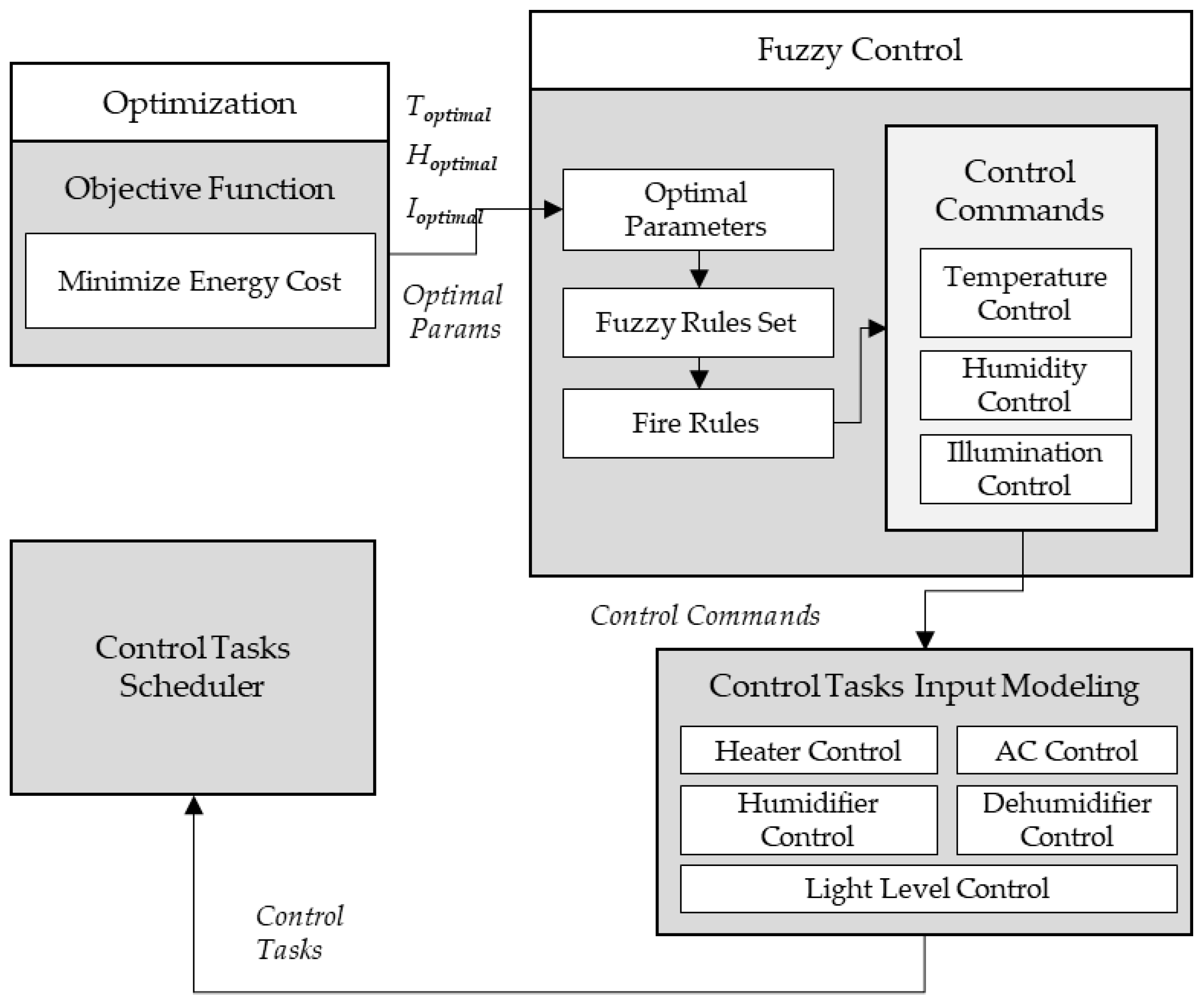
Once the optimal values are found, the optimal values are then used to derive fuzzy rules set to trigger the control commands based on input parameters to the fuzzy module.
Table 5 explains the actuator actions constraints based on which fuzzy control module generates the control rules for each actuator action. The control commands generated from the fuzzy control module are then used to model control tasks which are to be executed at the scheduler for control tasks’ operation (
Figure 6). We have used our previously implemented fuzzy control and scheduling module [
36] and made changes to fit our current scenarios.
6. Performance Analysis
In this section, first, we present the analysis of the results of predictions using multivariate LSTM algorithm with self-selected features. Then, we present the results analysis of predictions using multivariate LSTM algorithm with feature learning.
We use root mean square error (RMSE) measure as a performance metric to compare prediction performance. RMSE is the standard deviation of the residuals (prediction errors), where residuals are a measure of how far from the regression line data points are. In other words, it tells you how concentrated the data is around the line of best fit.
6.1. PredictionMechanism without Feature Learning
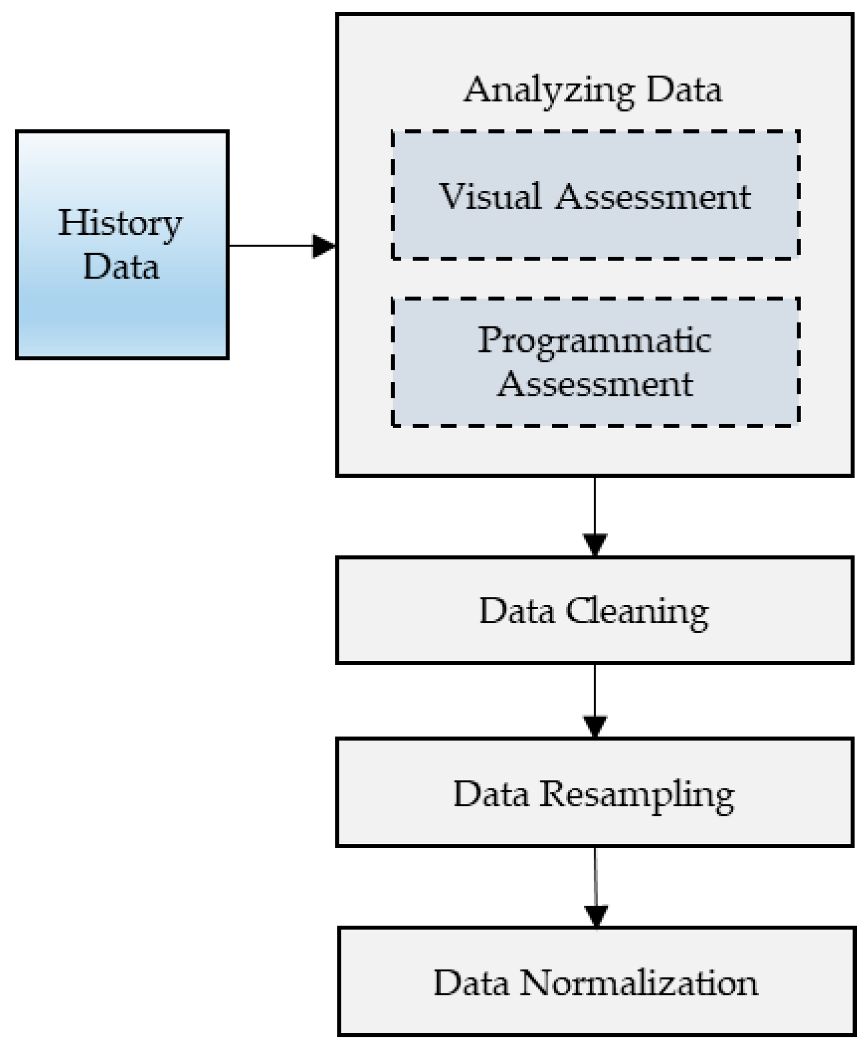
In this subsection, we perform predictions using self-selected contextual features. During the visual assessment and programmatic assessment, we observed the available features in the dataset. We studied the trends of each feature’s data values over the period of year through different seasons. After carefully studying data trends, we decided to drop the features that seemed irrelevant to the data. Initially, we had 11 contextual features of temperature, humidity, dew point, conditions, gust speed, precipitation mm, sea level pressure, visibility km, wind speed km/h, wind direction, and wind direction degrees. After dropping irrelevant features, we were left with eight contextual features: temperature, humidity, dew point, precipitation mm, sea level pressure, visibility km, wind speed km/h, and wind direction degrees. We further ranked eight contextual features into most to least relevant based on our data trends study and analysis. The ranking in descending order was as following: temperature, humidity, dew point, precipitation mm, visibility km, wind speed, sea level pressure, and wind direction degrees (
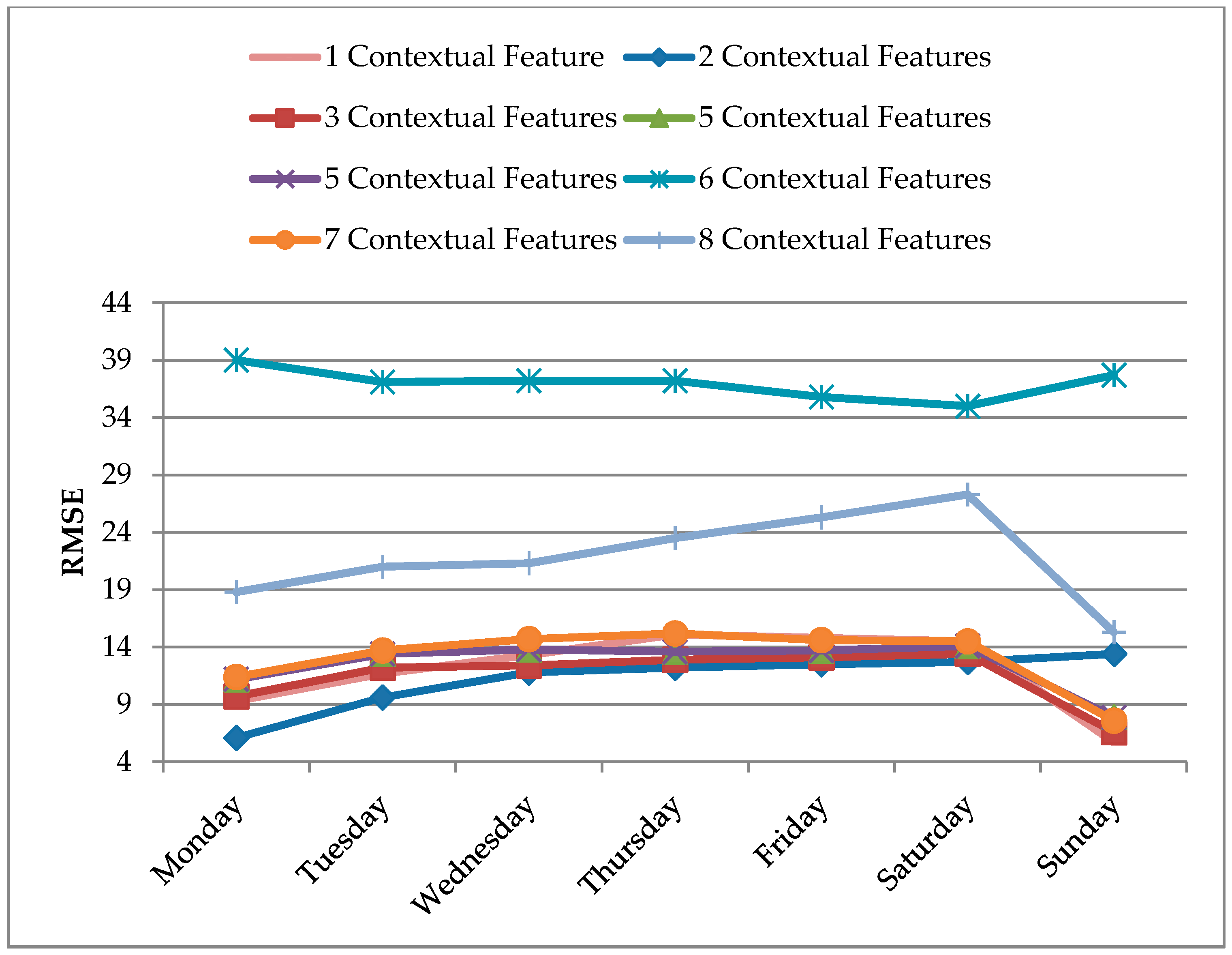
Table 8).
Figure 8 shows the weekly prediction results of all eight datasets. We can observe from the results that performance deviation does not necessarily align with our feature selection order. Though in some cases, removal of an irrelevant contextual feature (based on self-ranking) has shown improvement in the prediction performance such as from Dataset 8 to Dataset 7, but right in the next removal, from Dataset 7 to 6, the performance was badly affected as well. Similarly, a mixed effect on the prediction performance was observed for training and testing using Dataset 6 until Dataset 1.
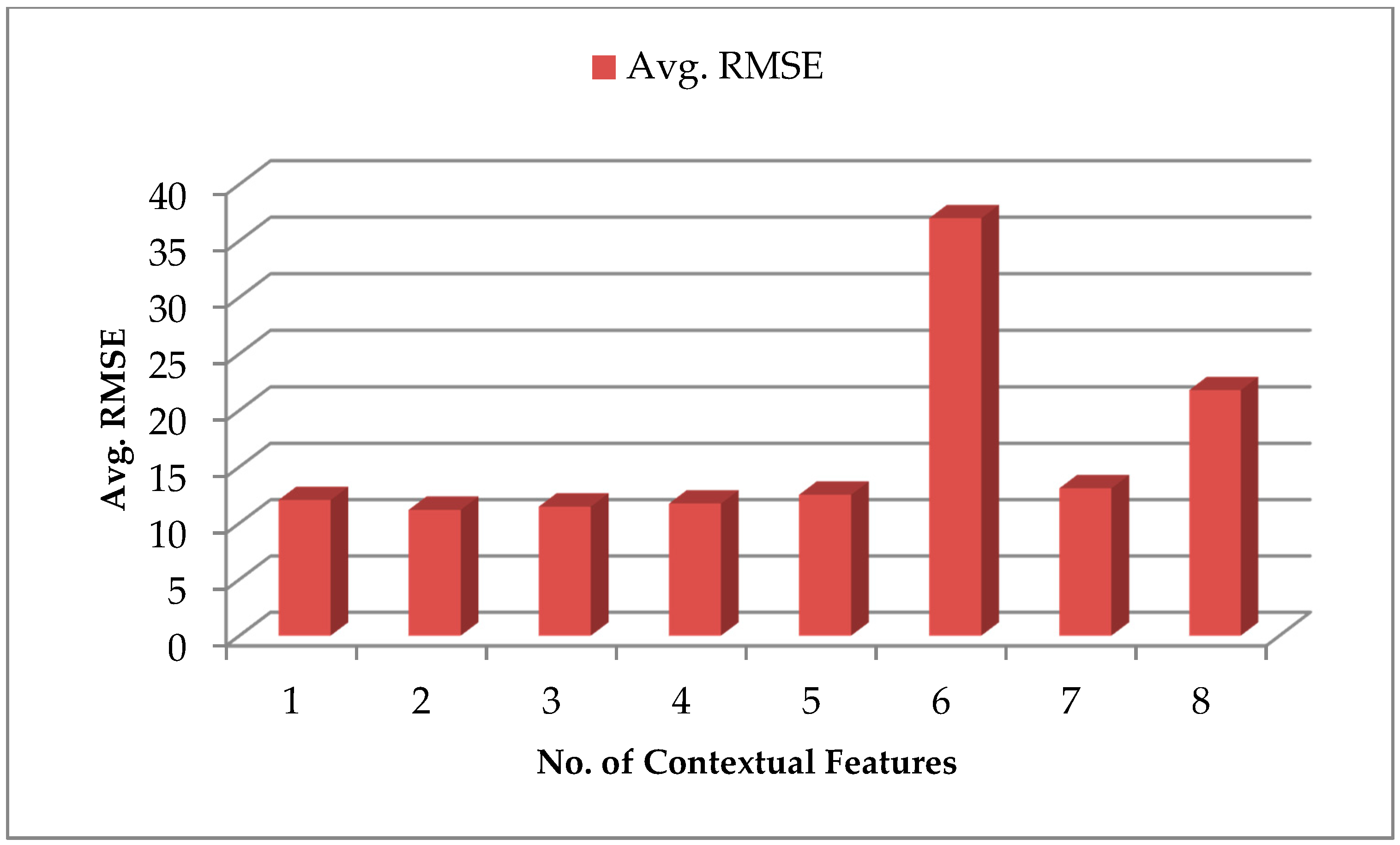
The average RMSE values for each dataset with a varying number of contextual features are given in
Figure 9. Our ranking of contextual features still proved to be relevant as best prediction performance observed with Dataset 2 containing two top-ranked contextual features. Still, the best prediction performance in this scenario had considerable deviations of predicted values from the actual values. Unless we derived datasets of all the contextual features’ combinations and trained and tested our prediction model with all datasets, we cannot be sure that the achieved results with the given Dataset 2 were the best results possible. Such regressive training with all the combinations of features still seems a doable task for datasets with fewer features; but as the number of features increases, it becomes very costly to train and test for all the possible combinations to find the best prediction results. Hence, in the next section, we observe the prediction results based on feature learning.
6.2. Prediction Mechanism with Feature Learning
In this subsection, we observe the prediction performance for multivariate LSTM algorithm with feature learning.
The model starts training with the entire dataset containing timestamp, energy, and 11 contextual features such as temperature, humidity, dew point, conditions, gust speed, precipitation mm, sea level pressure, visibility km, wind speed km/h, wind direction, and wind direction degrees. The model calculates feature relevance and learns feature relevance score based on features’ history relevance after each cycle. An updated set of features is used for predictions in the next cycle.
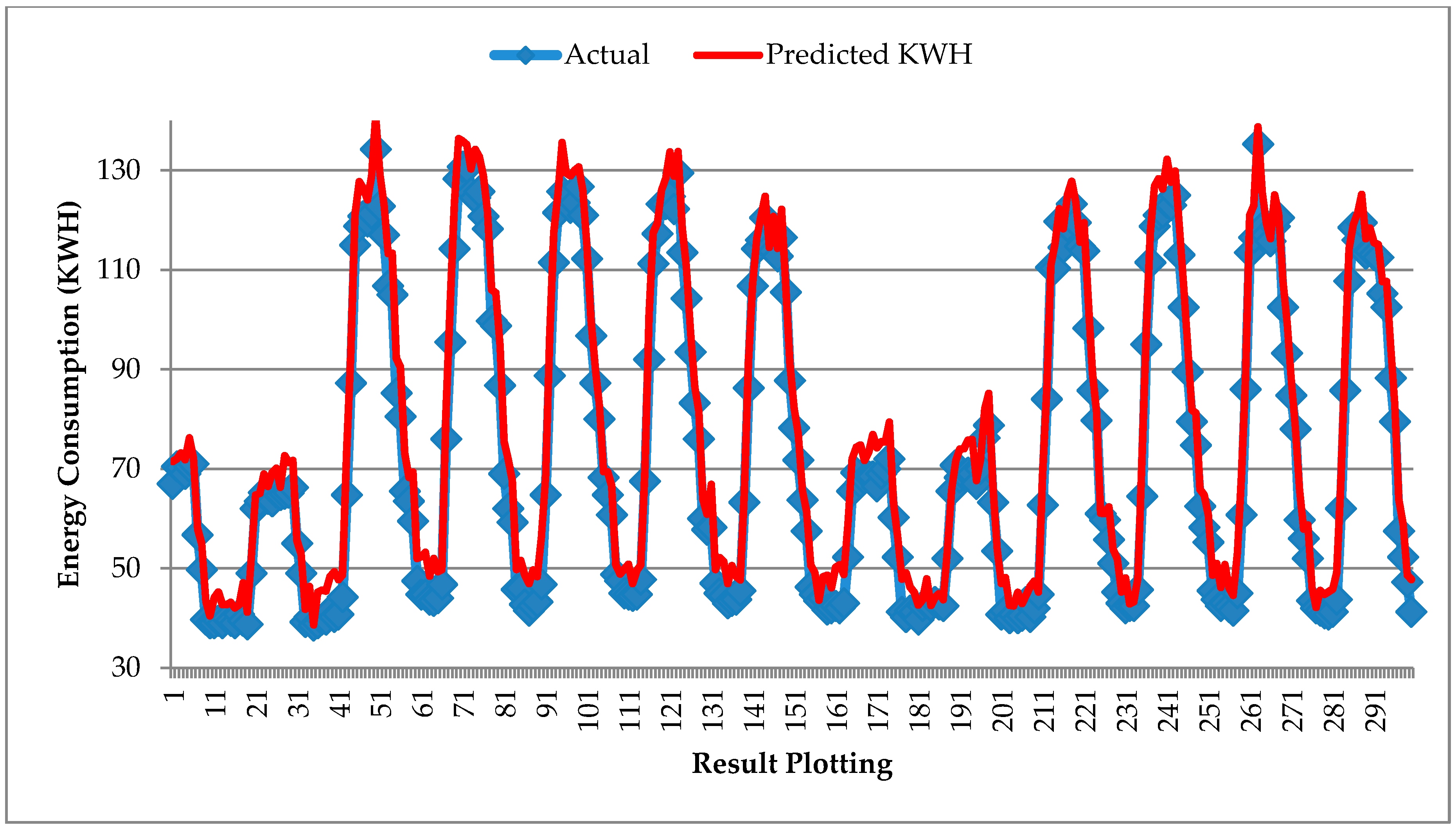
Figure 10 shows the prediction result plotting of predicted energy values against actual energy values. We can observe that deviations in the predicted results do not seem to be very high as compared to the previous best-achieved results with Dataset 2 in
Section 6.1.
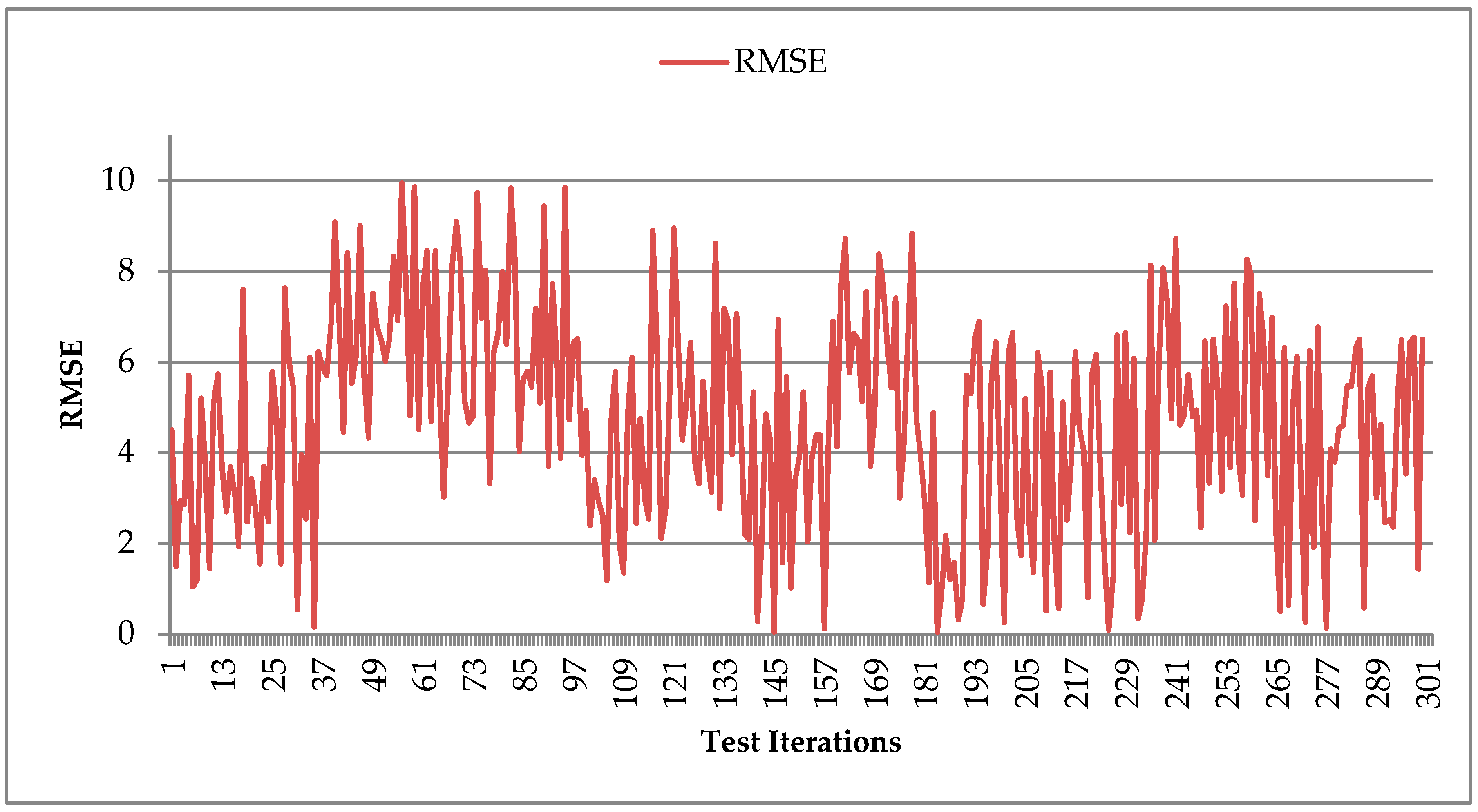
Figure 11 shows the RMSE score for the prediction results for LSTM with feature learning. The feature learning module updates the dataset based on calculated feature relevance. These prediction results were obtained after four cycles of LSTM algorithm training with feature learning adaptations. The average RMSE obtained was 4.70. We could observe that feature learning learns the most relevant feature very quickly, and also, the error between predicted values in contrast to actual values was reduced drastically.
If we consider finding the best combination of features without the feature learning approach, then we have to check for all the possible combinations of features. If we consider our scenario of 11 contextual features, then the possible number of contextual features’ combinations will be 2047. If we consider the self-selected contextual features, then the possible number of contextual features’ combinations will be 255. Even in the case of eight contextual features, the total number of training cycles to find the best possible prediction results will be costly at processing powers and more time-consuming. In the table below, we present the comparison analysis for prediction model results for running of possible combinations for X = 8 and X = 11 with the LSTM model; in comparison with the prediction performance results for our proposed feature learning-based adaptive LSTM approach (
Table 9).
6.3. Predictive Learning Based Optimal Control Mechanism
In this section, we examine the performance of a predictive learning-based optimal control mechanism. We perform the comparison analysis between optimal control mechanisms with predictive learning and without predictive learning.
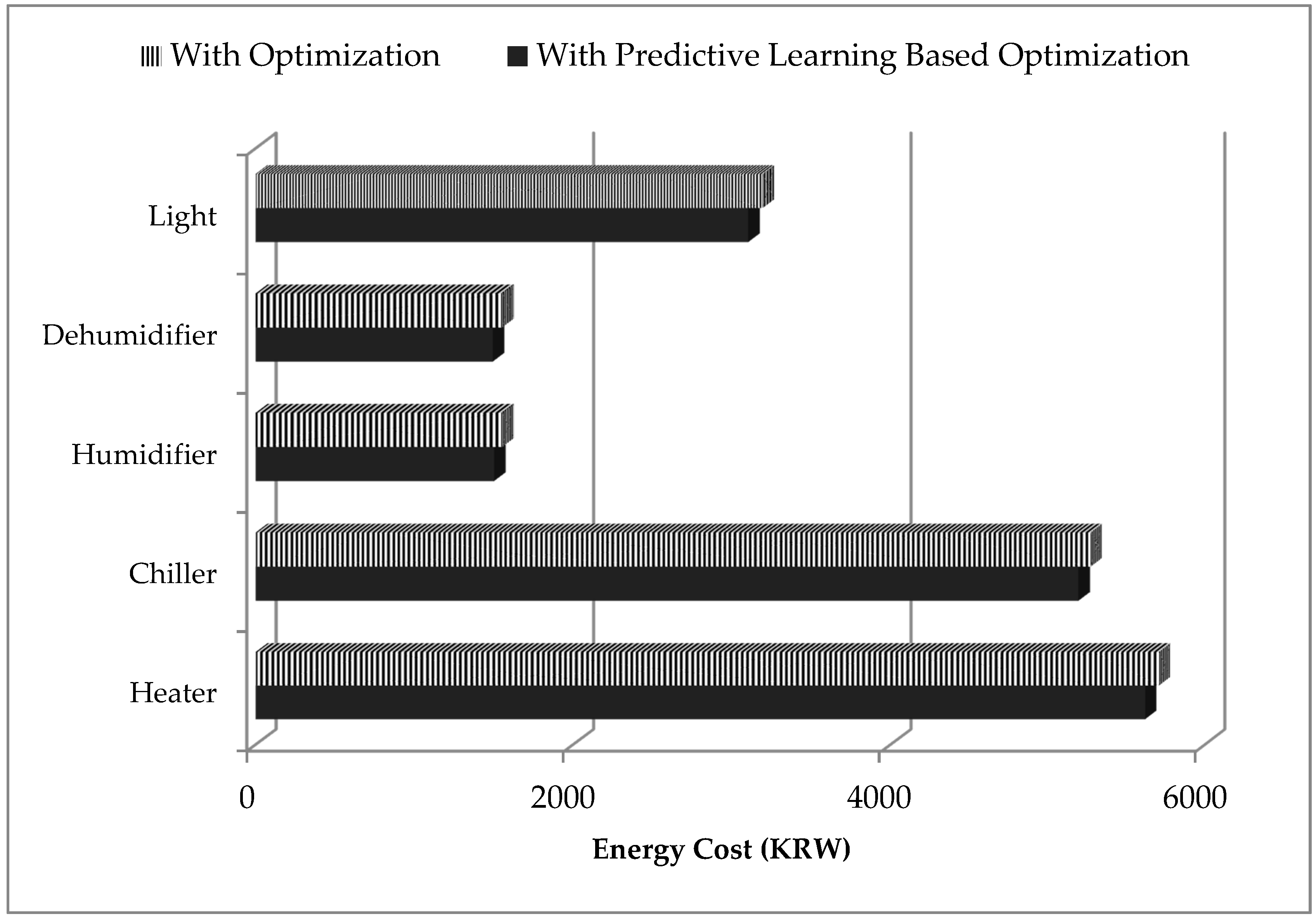
Figure 12 shows the comparisons of the results between predictive learning-based optimization scheme and nonpredictive learning-based optimization scheme. The y-axis shows the actuators which are being controlled at the smart home, and x-axis shows the energy consumption cost for actuator control. The energy consumption cost was measured in South Korean Won (KRW). In the results, we can clearly see that energy cost was optimized and reduced when a predictive learning-based optimization mechanism was used compared to the optimization mechanism where no predictive learning was implemented.
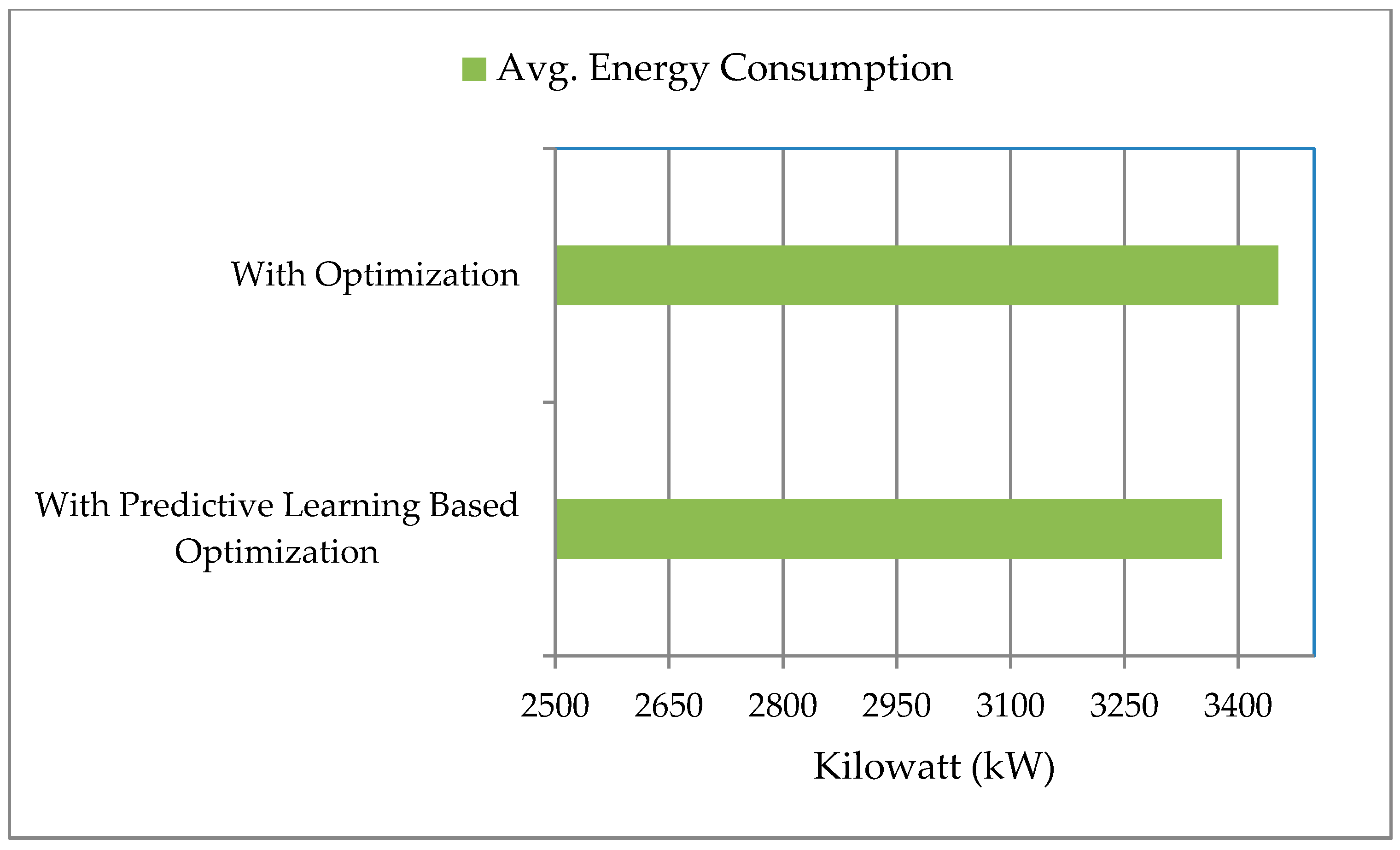
In
Figure 13, we present the comparison of average energy consumption for optimal actuator control with and without predictive learning. In the results, we can observe that average energy consumption was reduced with predictive learning-based optimization actuator control.
If we observe the above figures, we can see that in every actuator, we were getting improvement with our proposed predictive learning-based approach. Lights were 2.9% more cost-efficient, while dehumidifiers and humidifiers showed about 3% improvement in reducing the cost. Chiller and heater also showed about a 1.4% and 1.6% decrease in the consumption cost compared to other approaches (i.e., optimizations without predictive learning). All these comparisons are listed in
Figure 12. If we consider total energy consumption of the whole system, we again see our proposed scheme outperforming the default setup. Our proposed scheme consumed approximately 3378 kilowatts, while the default system consumed 3420 kilowatts. This gave us around 2.18% improvement over the existing system. The calculation is summarized in
Figure 13.
7. Conclusions
In this work, we presented a predictive learning-based optimal control mechanism for actuators deployed in smart environments. At first, we proposed a feature learning-based smart home energy prediction solution that aims to improve the prediction accuracies by filtering the contextual data based on history learnings. The algorithms used in the proposed mechanism were LSTM for energy predictions and ANN-PSO for feature learning within LSTM cycles. Our proposed prediction model takes all available features at the first cycle of energy prediction and works its way down to learn the most impactful features. The proposed model also learns to re-add features based on history learned relevance at a given prediction time. We used our implemented prediction module to further aid the optimization of a smart home actuators’ control mechanism. The optimization model performance was enhanced by adding the predictive learning mechanism to it. The integration of predictive learning with optimal actuator control aims to reduce energy consumption with less dependency on the user-defined parameters for optimal control.
When analyzing the result, we compared how feature learning can dramatically increase the prediction model’s performance. It finds the set of best suited contextual features with very few cycles of learning. The proposed solution can be very effective for scenarios where the dataset contains large numbers of features. It can help extract the most relevant features efficiently. Additionally, in many cases, researchers often work with datasets where they might not have complete knowledge of the data field. In such cases, the proposed model can also help researchers with feature learning and save a fair amount of time.
As the results demonstrate, our proposed system (i.e., predictive learning-based optimal control mechanism) clearly reduced the whole system’s energy consumption. Saving energy is of critical importance; hence, the proposed integration can largely benefit smart homes’ optimal actuator control systems.


