Adaptive Damping Variable Sliding Mode Control for an Electrohydrostatic Actuator

Abstract

An electrohydrostatic actuator (EHA) is a basic mechanical/hydraulic system with deficiencies including significant nonlinearity and parametric uncertainties. In line with the challenges of designing a high-precision control strategy, an adaptive damping variable sliding mode controller is established, which extends our previous work on EHA control. The proposed controller integrates variable-damping sliding mode control, parametric adaptation, and an extended state observer. The parametric uncertainties are effectively captured and compensated by employing an adaptive control law, while system uncertainties are reduced, and disturbances are estimated and compensated with a fast and stable response. We evaluated the proposed control strategy on a variety of position tracking tasks. The experimental results demonstrate that our controller significantly outperforms the widely used methods in overshoot suppression, settling time, and tracking accuracy.

1. Introduction

Flight-control actuation systems of more-/all-electric aircrafts must balance the requirements of high power, light weight, safety, fast response, and continuity of service. The trend toward using more electrical aircrafts can be gradually implemented by the employment of highly integrated electrical powering systems, i.e., electrohydrostatic actuators (EHAs) and electromechanical actuators (EMAs) [1,2]. With the removal of meter-in and meter-out valves as well as pipelines, both EHAs and EMAs improve the power density and minimize the system volume in a way that clearly outperforms conventional hydraulic systems [3].

According to current publications, an EMA has the simplest structure and provides the highest efficiency [4,5], whereas the high probability of jamming, together with the wear of mechanical transmission components, is most pronounced in EMA devices [6]. By contrast, EHAs have been adopted in the aerospace industry since early 2000 due to their superiority in terms of reliability and maintenance, and because they are environmentally friendly [7]. As at state-of-the-art Joint Strike Fighter, the F35 employs an EHA in its flight surface control system as the flat tail actuator [8,9]. It is highly significant that EHAs have already become the core components of more-/all-electric aircrafts [10,11].

However, the application of EHAs is still limited, primarily because of deficiencies such as time-variation parameters, system uncertainties, and the dead zone caused by cylinder leakage and friction [12]. For this reason, current research is ongoing that is aimed at paving a way to further improve the capabilities of EHAs. In the context of system establishment, control strategies have profound effects and give rise to better working performance. This decade has witnessed advances in control approaches to facilitate the operation of EHA. Specifically, a substantial theme of current control strategies is to upgrade the actuator robustness. In [13], Ren et al. propose a quantitative feedback theory-based controller that maintains a balance between stability, tracking, disturbance rejection, and parametric uncertainties. In order to deal with system disturbance and external noise, Zhang et al. fused the sliding mode and H∞ control to stabilize the EHA system [14]. Wang et al. carried out a deterministic robust control scheme, together with compensation of system uncertainties [15]. Experimental results confirm the effectiveness of the proposed controller depending on the use of adaptive control and observation of disturbances. Among these control strategies, adaptive robust control (ARC) has the highest precision in servo control despite the complexity of variables [16]. On the other hand, sliding mode control (SMC), as a preferred alternative, is widely applied due to its robustness in parametric variation and unmodeled dynamics. However, there is still a significant limitation for SMC: large control gain, along with the increased nonlinear robust items, as suppressing the uncertainties will cause chattering during steady phases. Thus, recent advancements highlight efforts to reduce system chattering of SMC in EHAs [17,18,19].

On the one hand, the result of step signals is introduced in [20], while the results of tracking sinusoidal input are not taken into consideration. On the other hand, performance degradation is inevitable because of the omission of feedforward items, i.e., the derivative of the reference that can be regarded as compensation. Further, an extended state observer (ESO) is designed for the estimation of all uncertainties, which leads to overburdening of the ESO.

Therefore, a novel adaptive damping variable sliding mode control (ADV-SMC) is proposed to tackle the aforementioned problems. An adaptive law driven by both tracking errors and state estimation errors is introduced. The task of the ESO is mitigated since the majority of parametric uncertainties can be suppressed by the adaptation law. Moreover, when tracking sinusoidal signals, the integration of the tracking error driven adaptation law alleviates the degradation caused by the missing feedforward items. Consequently, the effectiveness of the proposed controller can be guaranteed by merging ESO, adaptive law, and SMC.

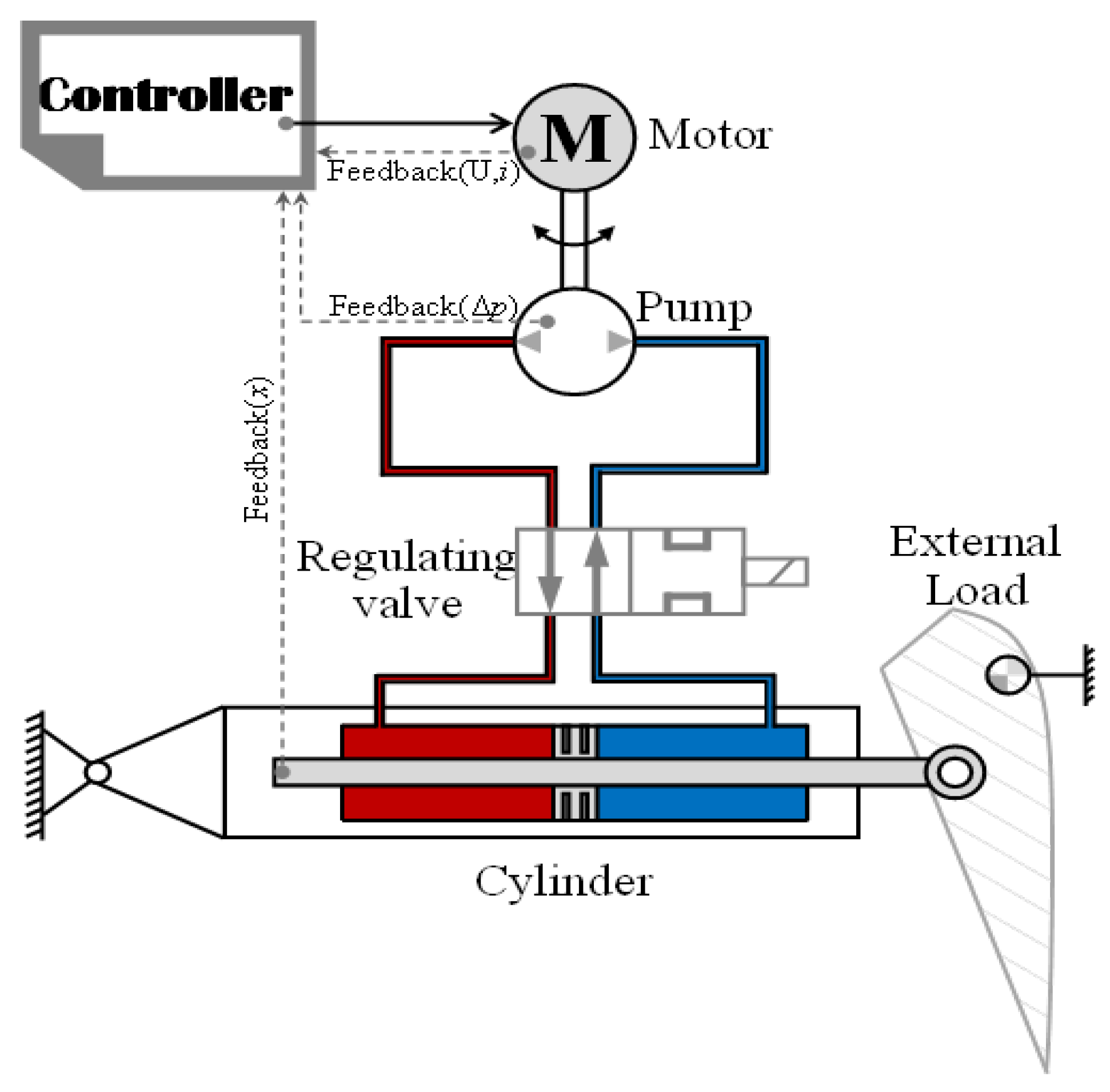
2. Mathematical Model of the EHA

Theoretically, the EHA is considered to be an integrated motor drive composed of a motor, a pump, a cylinder, and a supercharged fuel tank [21,22]. This actuating system is an integration of electric-to-mechanical and mechanical-to-hydraulic power conversion, as presented in Figure 1. The controller transmits the control command to the motor to drive the hydraulic pump by controlling its pressure and flow. The regulating valve switches the two oil paths according to the pressure of the oil circuit. That is, the cylinder, with the external load on its output end, extends and retracts in line with the absorbing and discharging of hydraulic oil. In essence, the plunger pump and servo motor are commonly used in EHA systems due to their high efficiency.

2.1. Modeling of the Brushless DC Motor (BLDCM)

A typical servo motor model is the brushless DC motor (BLDCM). In this case, the three windings are in a Y-connection. Assume that the parameters of each winding stay the same and the magnetic field between the stator and the rotor is a regular trapezoidal wave. The model of the motor winding is given as follows [23,24]:

$$\{\begin{array}{l}{U}_U=L_U{\dot{i}}_U+R_U{i}_U+e_U+U_N\\ U_V=L_V{\dot{i}}_V+R_V{i}_V+e_V+U_N\\ U_W=L_W{\dot{i}}_W+R_W{i}_W+e_W+U_N\end{array}$$

(1)

where the subscripts U, V, and W represent the three phases of the motor, $L_{*}$ is the phase inductance, $i_{*}$ is the phase current, $R_{*}$ is the phase resistance, $e_{*}$ is the back electromotive force (back-emf), and $U_N$ is the neutral-point voltage of the three-phase connection.

In most cases, the BLDCM works in a pairwise conduction mode, based on which Equation (1) can be rewritten as:

$$U=L\dot{i}+Ri+E$$

(2)

where $U$, $L$, $i$, $R$, and $E$ are equivalent voltage, inductance, current, resistance, and back-emf of the BLDCM, respectively.

Let $K_t$ be the torque coefficient of the BLDCM. The dynamic equation of the rotating motor can be:

$$\{\begin{array}{l}U=L\dot{i}+Ri+K_e\omega \\ T_e=K_{t}i\\ J_m\dot{\omega }=T_e-T_L-B_m\omega \end{array}$$

(3)

where $K_e$ stands for the back-emf coefficient, $T_e$ indicates the BLDCM electromagnetic torque, $J_m$ is the moment of inertia of the motor, $T_L$ is the equivalent external load, and $B_m$ is the coefficient of viscous friction.

2.2. Modeling of Pump and Cylinder

Based on the working principle of a hydraulic pump, the inlet flow $Q_i$ and outlet flow $Q_o$ of the plunger pump can be presented as:

$$\{\begin{array}{l}{Q}_i=\omega D_p-L_i(p_i-p_o)-L_o(p_i-p_a)-\frac{V_{in}}{{\beta }_e}{\dot{p}}_i\\ Q_o=\omega D_p-L_i(p_i-p_o)+L_o(p_o-p_a)+\frac{V_{out}}{{\beta }_e}{\dot{p}}_o\end{array}$$

(4)

where $D_p$ is the pump displacement; $L_i$ and $L_o$ represent the internal and external leakage coefficients; $p_i$, $p_o$, and $p_a$ are inlet pressure, outlet pressure, and back pressure from the oil tank; $V_{in}$ and $V_{out}$ are equivalent inlet and outlet volume; and ${\beta }_e$ is the elastic modulus of fluid.

Likewise, the dynamic model of the cylinder is:

$$\{\begin{array}{l}{Q}_l=A\dot{x}+\frac{V_{in}}{{\beta }_e}\frac{d{p}_l}{dt}+L_c(p_l-p_r)\\ Q_r=A\dot{x}-\frac{V_{out}}{{\beta }_e}\frac{d{p}_r}{dt}-L_c(p_l-p_r)\end{array}$$

(5)

where the subscripts $l$ and $r$ denote the left and right side of the cylinder chambers, and $A$ is the effective area of the piston rod, with $x$ representing its displacement. $L_c$ indicates internal leakage.

Let:

$$Q_l=Q_i,Q_r=Q_o$$

in line with the negligible pressure loss within the valve and the flow continuity theorem. We can obtain the models of the pump and the cylinder with:

$$\{\begin{array}{l}{D}_p\omega =A\dot{x}+\frac{V_0}{{\beta }_e}\Delta \dot{p}+L_a\Delta p+Q_a\\ A\Delta p=M\ddot{x}+B_c\dot{x}+K_{s}x+F_f+F_L\end{array}$$

(6)

where $V_0$ is the effective volume of the chamber, $L_a$ is the total leakage coefficient of the pump and the cylinder and is proportional to the pressure difference. $\Delta p$, $Q_a$ is the unconsidered flow loss within the system, $M$ denotes the equivalent mass of the cylinder and the external load, $B_c$ is the viscous friction coefficient of the cylinder, $K_s$ is the elastic load coefficient, $F_f$ is the static friction, and $F_L$ is the external load.

At this stage, we can define vector $X={[x_1{x}_2{x}_3{x}_4{x}_5]}^T={[x\dot{x}\Delta p\omega i_q]}^T$ to characterize the system state. Then the EHA model is defined as:

$$\{\begin{array}{l}{\dot{x}}_1=x_2\\ {\dot{x}}_2=\frac{A}{M}{x}_3-\frac{K_s}{M}{x}_1-\frac{B_c}{M}{x}_2-\frac{F_f+F_L}{M}\\ {\dot{x}}_3=\frac{{\beta }_e}{V_0}(D_p{x}_4-A{x}_2-L_c{x}_3-Q_{un})\\ {\dot{x}}_4=\frac{1}{J_a}(K_t{x}_5-B_m{x}_4-D_p{x}_3-T_f)\\ {\dot{x}}_5=\frac{1}{L}(U-R{x}_5-K_e{x}_4)\end{array}$$

(7)

where $J_a$ is the total rotational inertia of the motor and the pump and $Q_{un}$ indicates the unconsidered system flow loss. Notably, an EHA can be considered as a high-order system that takes bus voltage U as the input and piston displacement x1 as the output, with the nonlinear and mismatched disturbances.

3. Adaptive Damping Variable Sliding Mode Control Strategy

3.1. Problem Formulation

As presented in Equation (7), the first two formulas refer to the dynamics of the hydraulic cylinder, the third characterizes the system pressure, and the last two indicate the rotating speed and electric current of the motor. If, and only if, x4 is the input u of the first three formulas, the EHA model is subdivided into two inertia parts, the mechanical–hydraulic side and the motor side. The former has the input of motor speed and the output of cylinder displacement, and the latter has the input of bus voltage and the output of motor speed.

Note that mismatched disturbance exists within the mechanical–hydraulic side when classical sliding mode control is incapable of dealing with it. We thus transform the mechanical–hydraulic side before establishing the controller. The state variables of the mechanical–hydraulic side are redefined as:

$$Z={[z_1,z_2,z_3]}^T={[x_1,{\dot{x}}_1,{\ddot{x}}_1]}^T$$

(8)

together with the three-order state model of the mechanical–hydraulic side as:

$$\{\begin{array}{l}{\dot{z}}_1=z_2\\ {\dot{z}}_2=z_3\\ {\dot{z}}_3=g(z_3,z_2,z_1,u,F_f,F_L)\end{array}$$

(9)

and the redefined state variables delivered as:

$$\{\begin{array}{l}{z}_3={\dot{x}}_2=\frac{A}{M}{x}_3-\frac{K_s}{M}{x}_1-\frac{B_c}{M}{x}_2-\frac{F_f+F_L}{M}\\ M{\dot{z}}_3=A{\dot{x}}_3-K_s{z}_1-B_c{z}_2-d(F_f+F_L)/dt\end{array}$$

(10)

Computation with Equation (10) is facilitated by substituting Equation (7) into it:

$$\begin{array}{l}M{\dot{z}}_3=A[\frac{{\beta }_e}{V_0}(D_p{x}_4-A{x}_2-L_c{x}_3-Q_{un})]\\ -K_s{z}_1-B_c{z}_2-d(F_f+F_L)/dt\end{array}$$

(11)

The combination of first formula from Equations (10) and (11) yields:

$$\{\begin{array}{l}{\dot{z}}_1=z_2\\ {\dot{z}}_2=z_3\\ g_3{\dot{z}}_3=u-A_3{z}_3-A_2{z}_2-A_1{z}_1+f_d(t)\end{array}$$

(12)

where:

$$\begin{gathered} g_3=M{V}_0{(A{\beta }_e{D}_p)}^{-1} \\ {A}_3=L_{c}M{(A{D}_p)}^{-1} \\ {A}_2=L_c{B}_c{(A{D}_p)}^{-1}+A{D}_p{}^{-1}+B_c{V}_0{(A{\beta }_e{D}_p)}^{-1} \\ {A}_1=K_s{L}_c{(A{D}_p)}^{-1}+K_s{V}_0{(A{\beta }_e{D}_p)}^{-1} \end{gathered}$$

And:

$$f_d(t)=-Q_{un}{D}_p{}^{-1}-V_0({\dot{F}}_f+{\dot{F}}_L){(A{\beta }_e{D}_p)}^{-1}-L_c(F_f+F_L){(A{D}_p)}^{-1}$$

Specifically, the parameters $Q_{un}$, ${\dot{F}}_f$, and ${\dot{F}}_L$ are all considered bounded values.

At this point, the ADV-SMC strategy, consisting of an extended state observer (ESO) and an adaptive damping variable sliding mode controller, is designed and deployed.

3.2. Nonlinear Projection Mapping

Let ${\widehat{\theta }}_i$ denote the estimation of ${\theta }_i(i=1,2,3)$. A discontinuous projection Proj(*) is defined as:

$${\mathrm{Proj}}_{{\widehat{\theta }}_i}({•}_i)=\{\begin{array}{l}0,\mathrm{if}{\widehat{\theta }}_i>{\theta }_{i\max }\mathrm{and}{\dot{\widehat{\theta }}}_i>0\\ 0,\mathrm{if}{\widehat{\theta }}_i<{\theta }_{i\min }\mathrm{and}{\dot{\widehat{\theta }}}_i<0\\ •,\mathrm{else}\end{array}$$

(13)

Thus, the adaptation law $\dot{\widehat{\theta }}$ is:

$$\dot{\widehat{\theta }}={\mathrm{Proj}}_{\widehat{\theta }}(\mathsf{\Gamma }\vartheta ),{\theta }_{\min }<\dot{\widehat{\theta }}<{\theta }_{\max }$$

(14)

where $\mathsf{\Gamma }$ is a positive diagonal adaption gain matrix, and the adaptive function $\vartheta$ will be synthesized later. Consequently, for any function $\vartheta$ applying the nonlinear projection Proj(*), we have [25]:

$$\{\begin{array}{l}\widehat{\theta }\in {\mathsf{\Omega }}_{\widehat{\theta }}=\widehat{\theta },{\theta }_{\min }<\dot{\widehat{\theta }}<{\theta }_{\max }\\ \tilde{\theta }[{\mathsf{\Gamma }}^{-1}{\mathrm{Proj}}_{\widehat{\theta }}(\mathsf{\Gamma }\vartheta )-\vartheta ]\le 0\end{array}$$

(15)

with $\tilde{\theta }=\widehat{\theta }-\theta$.

3.3. Design of the Extended State Observer (ESO)

As described in the Introduction, an ESO is developed to estimate the unmeasurable disturbance and to relieve the burden on the robust items. In terms of this system, the state parameter available is $z_1$, which is detected directly by a displacement sensor. By contrast, $z_2,z_3$ are to be estimated. Let ${\widehat{z}}_1,{\widehat{z}}_2$ and ${\widehat{z}}_3$ be the estimations of $z_1,z_2$ and $z_3$, respectively. We also construct $z_4$ as an additional extended variable to denote the system disturbance. Concretely, the parameters A1, A2, A3, and g3 represent parametric uncertainties and are determined by the ARC scheme, while $f_d(t)$ represents the system disturbance observed in Equation (12).

The designed ESO is written as:

$$\{\begin{array}{l}{\dot{\widehat{z}}}_1={\widehat{z}}_2+\tau l_1(z_1-{\widehat{z}}_1)\\ {\dot{\widehat{z}}}_2={\widehat{z}}_3+{\tau }^2{l}_2(z_1-{\widehat{z}}_1)\\ g_3{\dot{\widehat{z}}}_3=u+{\widehat{\theta }}^{T}Z+{\widehat{f}}_d(t)+{\tau }^3{l}_3(z_1-{\widehat{z}}_1)\\ {\dot{\widehat{f}}}_d(t)={\tau }^4{l}_4(z_1-{\widehat{z}}_1)\end{array}$$

(16)

where $0<\tau$, while $L_{i(i=1,2,3,4)}=[l_1,l_2,l_3,l_4]$ is the observer gain and is a Hurwitz parameter. The definition of ${\widehat{\theta }}^T$ is shown later.

Subtracting (16) from (9) gives the observer error dynamics:

$$\dot{\chi }=\tau B_1\chi -\frac{B_2{\tilde{\theta }}^{T}Z}{g_3{\tau }^2}+\frac{B_{3}h(t)}{{\tau }^3}$$

(17)

where $h(t)$ is the dynamic of $f_d(t)$ and is unknown but bounded. Furthermore, $\chi ={[{\tilde{z}}_1,{\tilde{z}}_2/\tau ,{\tilde{z}}_3/{\tau }^2,{\tilde{f}}_d(t)/\tau ]}^T$, $B_2={[0,0,1,0]}^T$, $B_3={[0,0,0,1]}^T$, and:

$$B_1=\left[\begin{array}{cccc}-l_1& 1& 0& 0\\ -l_2& 0& 1& 0\\ -l_3& 0& 0& 1\\ -l_4& 0& 0& 0\end{array}\right]$$

Since matrix B₁ is a Hurwitz matrix, a positive definite matrix P satisfying $B_1^{T}P+P{B}_1=-I$ must exist and I is an identity matrix.

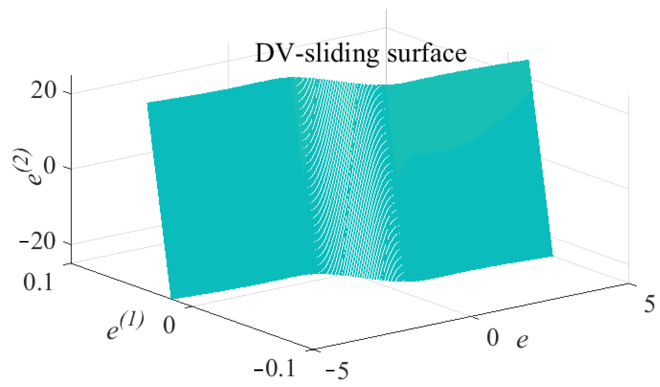
3.4. Design of the Adaptive Damping Variable Sliding Mode Controller (ADV-SMController)

Establishing an ADV-SMController starts with redefining the adaptive parameters: as

$$\theta ={[{\theta }_1,{\theta }_2,{\theta }_3]}^T={[A_1,A_2,A_3]}^T$$

(18)

In this way, Equation (12) can be rewritten as:

$$\{\begin{array}{l}{\dot{z}}_1=z_2\\ {\dot{z}}_2=z_3\\ g_3{\dot{z}}_3=u-\theta Z+f_d(t)\end{array}$$

(19)

System error e and its derivatives are defined as:

$$\{\begin{array}{l}e=e_1=z_1-x_d\\ \dot{e}=e_2=z_2-{\dot{x}}_d\\ \ddot{e}=e_3=z_3-{\ddot{x}}_d\end{array}$$

(20)

where x_d stands for the targeted tracking position of the system.

We define the damping variable (DV) sliding surfaces as follows [20]:

$$\{\begin{array}{l}{\sigma }_1=\ddot{e}+{\gamma }_t\dot{e}+{\omega }_n^{2}e\\ {\gamma }_t(e)=2{\omega }_n({\xi }_{\min }+\frac{{\xi }_{\max }}{1+\delta e^2})\end{array}$$

(21)

Based on the theory of SMC, it is designed to allow the sliding surface to reach convergence and ensure the parameters to be Hurwitz. As presented in Figure 2, one can easily see that the proposed DV sliding surface is nonlinear and varies according to the state of system error. According to our previous work [20], the sensitivity factor, together with the minimum and maximum damping ratios, also has an impact on the shape of the sliding surface.

The constant reaching law is applied on the reaching phase of the controller, which leads to:

$${\dot{\sigma }}_1=\eta sign({\sigma }_1)$$

(22)

and a finite-time convergence:

$$t_r=\left|{\sigma }_1(0)\right|/\eta$$

(23)

where t_r is the time interval to reach the sliding surface.

For the ADV-SMC strategy, the control input u₁, together with the parametric adaption, is devised as:

$$\{\begin{array}{l}{u}_1={\widehat{\theta }}_4{\stackrel{⃛}{x}}_d+\widehat{\theta }Z-{\widehat{f}}_d(t)-{\gamma }_t\ddot{e}-{\dot{\gamma }}_t\dot{e}-{\omega }_n^2\dot{e}-\eta sign({\sigma }_1)\\ \dot{\widehat{\theta }}=\mathrm{Proj}(-\mathsf{\Gamma }\vartheta )\end{array}$$

(24)

where:

$$\vartheta =-\frac{{\sigma }_1}{g_3}Z+{\chi }^{T}P{B}_2\frac{Z}{g_3{\tau }^3}$$

(25)

Notably, the control law has to use the estimated value $\widehat{\theta }$ rather than $\theta$ since it is impossible to obtain the true values of certain system parameters (e.g., cylinder damping coefficient, leakage coefficient, etc.).

3.5. Stability Analysis

To analyze the stability of the proposed control strategy, consider a Lyapunov function, given as:

$$V=\frac{1}{2}{\sigma }_1{}^2+\frac{1}{2}{\tilde{\theta }}^T{\mathsf{\Gamma }}^{-1}\tilde{\theta }+\frac{1}{2}{\chi }^{T}P\chi$$

(26)

where ${\mathsf{\Gamma }}^{-1}$ is the gain matrix of the controller and θ is a slow-change parameter.

During sliding, the differentiation of Equation (26) to time becomes:

$$\begin{array}{l}\dot{V}={\sigma }_1{\dot{\sigma }}_1+{\tilde{\theta }}^T{\mathsf{\Gamma }}^{-1}\dot{\widehat{\theta }}+\frac{1}{2}({\dot{\chi }}^{T}P\chi +{\chi }^{T}P\dot{\chi })\\ ={\sigma }_1[{\gamma }_t\ddot{e}-{\dot{\gamma }}_t\dot{e}-{\omega }_n^2\dot{e}+\frac{1}{g_3}(u-{\theta }^{T}Z+f_d(t)-{\stackrel{⃛}{x}}_d)]\\ +{\tilde{\theta }}^T{\mathsf{\Gamma }}^{-1}\dot{\widehat{\theta }}-\frac{1}{2}\tau {\Vert \chi \Vert }^2-{\chi }^{T}P{B}_2\frac{{\tilde{\theta }}^{T}Z}{g_3{\tau }^2}+{\chi }^{T}P{B}_3\frac{h(t)}{{\tau }^3}\\ =\frac{-\eta \left|{\sigma }_1\right|-{\tilde{f}}_d(t){\sigma }_1}{g_3}-\frac{1}{2}\tau {\Vert \chi \Vert }^2+{\chi }^{T}P{B}_3\frac{h(t)}{{\tau }^3}\\ \le \underset{1\mathrm{st}\mathrm{part}}{\underbrace{[-\eta +{\tilde{f}}_d(t)]\frac{\left|{\sigma }_1\right|}{g_3}}}-\underset{2\mathrm{nd}\mathrm{part}}{\underbrace{\frac{1}{2}\tau \Vert \chi \Vert (\Vert \chi \Vert -2\Vert P{B}_3\Vert \frac{{\left|h(t)\right|}_{\max }}{{\tau }^4})}}\end{array}$$

(27)

As presented in Equation (27), the first part denotes the convergence of the sliding surface and the second part denotes the convergence of observer error. If $\Vert \chi \Vert >2\Vert P{B}_3\Vert \frac{{\left|h(t)\right|}_{\max }}{{\tau }^4}$, then the second part is less than 0. In this way, $\Vert \chi \Vert$ is bounded by $\Vert \chi \Vert \le 2\Vert P{B}_3\Vert \frac{{\left|h(t)\right|}_{\max }}{{\tau }^4}$. If $\left|h(t)\right|=0$ ($f_d(t)$ given as a constant value), then the second part equals 0, which indicates that even a small gain coefficient η ensures the asymptotic stability of the system. If $\left|h(t)\right|\ne 0$, the bounded $\Vert \chi \Vert$ results in bounded $\left|{\tilde{f}}_d(t)\right|$. Once $\eta >\left|{\tilde{f}}_d(t)\right|$, all parameters within the system are bounded, and their upper bounds can be adapted by changing gain $\tau$.

Clearly, there is a $\tilde{\theta }$→0 for each trajectory slide along the surface, which assures $\dot{V}({\sigma }_1,\tilde{\theta })\le 0$, hence stable performance.

In order to prevent chattering while the sliding mode is approaching the steady state, the function sign (*) is described as:

$$sign(*)=\{\begin{array}{l}1,\mathrm{if}(*\ge 1)\\ *,\mathrm{if}(-1<*<1)\\ -1,\mathrm{if}(*\le -1)\end{array}$$

(28)

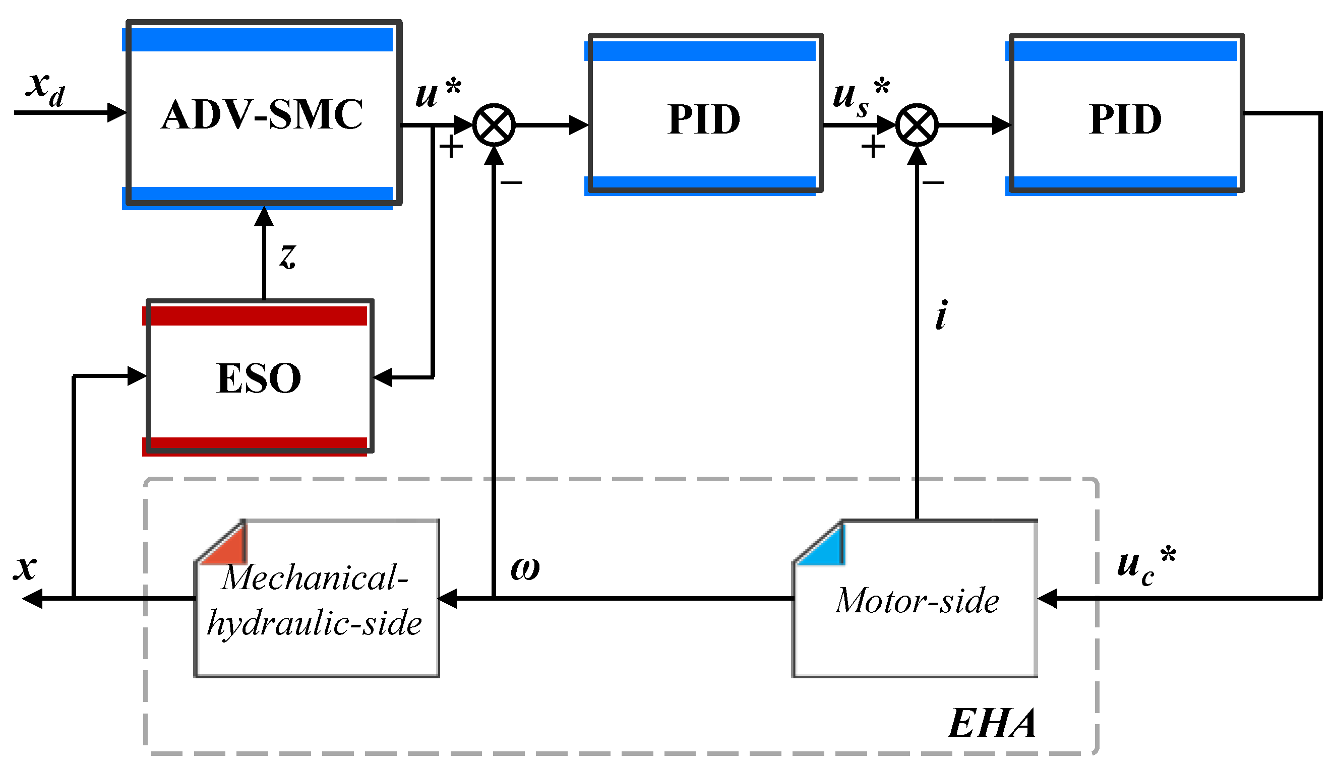
3.6. Control Method Design of the EHA

According to the working principle of the EHA, the motor control, with its input of voltage and output of motor spindle speed, is conducted by traditional double-loop proportion integration differentiation (PID).

$$\{\begin{array}{l}{u}_{id}=k_{ip}{e}_s+k_{ii}{\displaystyle \int e_{s}dt+k_{id}{\dot{e}}_s}\\ u_{Vd}=k_{Vp}{e}_i+k_{Vi}{\displaystyle \int e_{i}dt+k_{Vd}{\dot{e}}_i}\end{array}$$

(29)

In Equation (29), $u_{cd}$ and $u_{Ud}$ represent the target values of motor current and motor bus voltage; $k_{*p},k_{*i},k_{*d}$(* = i, V) are the proportional coefficient, integral coefficient, and differential coefficient for PID control; and $e_s,e_i$ represent the speed deviation and current deviation, respectively.

With the integration of the ADV-SMC strategy, a cascade controller is established where the outer loop is an ADV-SMController and the inner loop is a double-loop PID controller (Figure 3).

It is clear that we have the motor side and the mechanical–hydraulic side connected in series. Conforming to the dominant pole, this implies that the motor side can be considered as a proportional component when its dynamic response is much faster than the mechanical–hydraulic side [15]. When implementing the system practically, the proposed controller establishes stable performance under the condition that the motor dynamics are much higher than the cylinder dynamics. Equation (19) gives the proof of control stability.

4. Experimental Verification

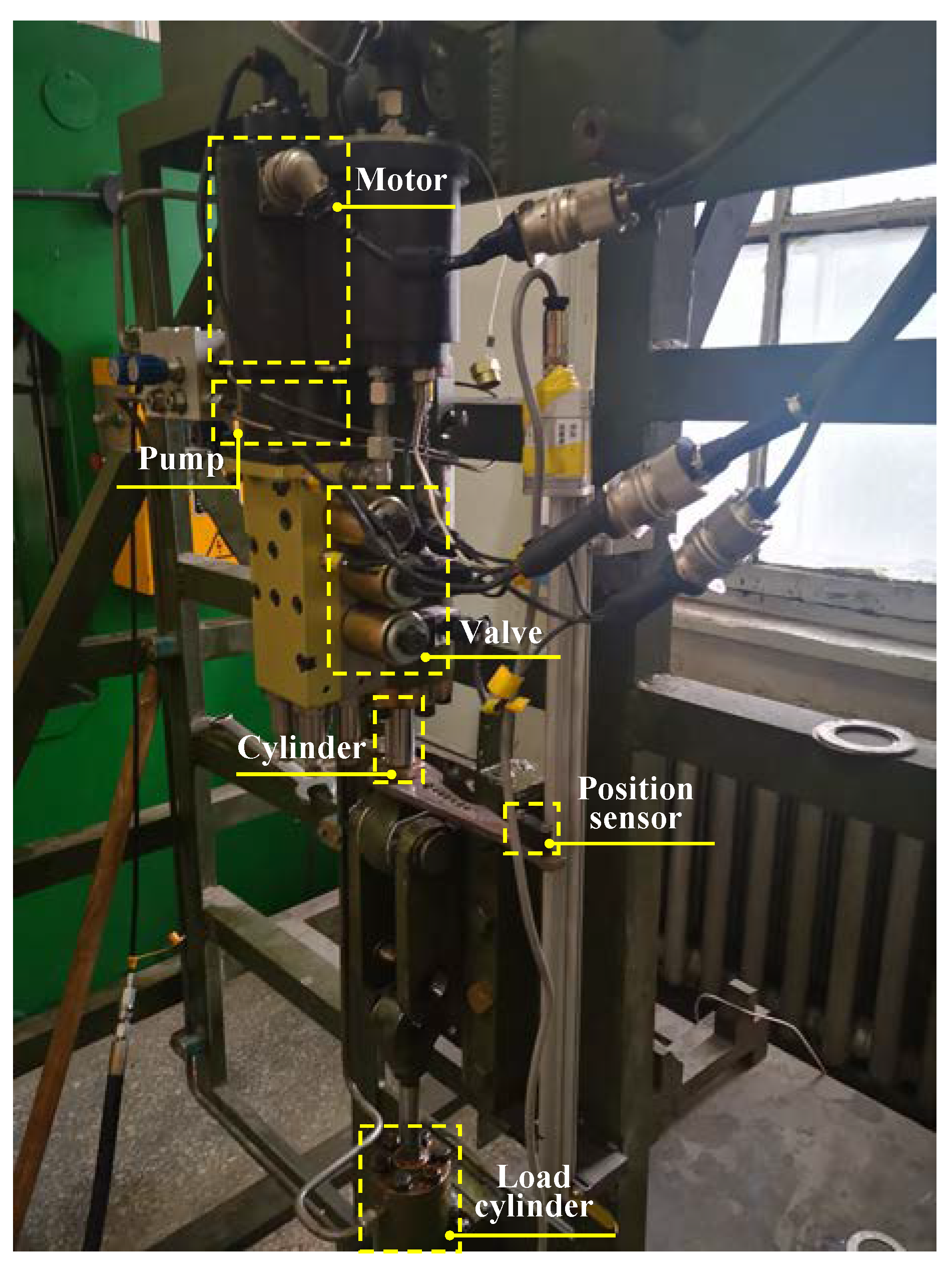
4.1. Experimental Setup

A photograph of the testing rig is shown in Figure 4. An EHA prototype is mounted on a platform. The control commands are configured to run the motor in rotating speed control mode with analog inputs and further drive the pump. The regulating valves are mounted directly beneath the pump to switch the working mode. An encoder is embedded alongside the cylinder to detect position data, based on which the displacement of the actuator is determined. Details of the EHA parameters are presented in

Table 1. Specifications of the EHA.

Parameter	Value
Piston effective area (m2)	1.134 × 10−4
Effective stroke (m)	0.1
Fluid elastic modulus (N/m2)	6.86 × 108
Hydraulic cylinder volume (m3)	4 × 10−4
Mass of cylinder and load (kg)	243
Pump displacement (m3/rad)	3.98 × 10−7
Phase resistance (Ω)	0.2
Phase inductance (mH)	1.33
Motor spindle moment of inertia (kg⸱m2)	4 × 10−4
Torque coefficient (N⸱m/A)	0.351
Back EMF coefficient (V/(rad/s))	0.234
Bus voltage (V)	270

.

ADV-SMC is performed to control the EHA via the control commands and state feedback. During testing, power electronics provide a real-time interaction for measurement and control. The motor is controlled using motor driving signals, while the feedback, containing the motor current and cylinder displacement, is captured using sensing elements. The sampling time of control is 0.5 ms and the feedback is derived from a second-order Butterworth filter with a 40 Hz cut-off frequency. An external load of 5000 N is applied to the EHA to implement the control strategy. In order to verify the effectiveness of the proposed controller, the following methods are taken for comparison:

PID: The PID controller gives accurate position control that is stable and easy to perform. In the experiments, the related controller gains are tuned carefully by trial and error to kp = 65,000, ki = 48,500, and kd = 0.

SMC: The basic SMC strategy is robust to parameter variation and unmodeled dynamics. The parameters are designed as follows: c1 = 70.7, c2 = 2500, and η_SMC = 210.7, which are determined via online tuning to facilitate the implementation.

DV-SMC: This is based on a previous study of an improved SMC strategy aiming to suppress the overshoot and provide a rapid response. We set the parameters the same as in [20]: δ = 1, ω_n = 50, ξ_max = 1, ξ_min = 0.1, η_DV-SMC = 210.7.

Specifically, the proposed ADV-SMController, which is established based on DV-SMC, employs the gain matrix Γ = diag{105, 2.2 × 10³, 25}, which is also determined via online tuning. The variable θ is bounded by θ_max = [10, 5000, 25] and θ_min = [0, 1000, 0]. In addition, the initial estimate is set as $\widehat{\mathsf{\theta }}=[1,2000,5]$. Other parameters are the same as those for DV-SMC.

All of the aforementioned methods are the outer loop of the cascade controllers, while the inner loop is a double-loop PID controller. To comprehensively evaluate the performance, these four controllers are tested for two step trajectories and a sinusoidal trajectory, which refer to all working conditions of the EHA in practical use.

4.2. Results

To start, step signals of 5 and 50 mm are applied as references to generate the system responses. The position tracking results are shown in Figure 5 and Figure 6. Generally, PID and classical SMC strategies generate overshoots in line with both step signals. By contrast, the variable damping-based methods, DV-SMC and ADV-SMC, have superiority in suppressing the overshoot and obtaining a stable response. Comparing DV-SMC and ADV-SMC with the disturbance compensation of the ESO, ADV-SMC converges to the reference at a higher speed.

To expand, for working property characterization, we can use the following definitions:

Settling time (ST): The first time stabilizing within the range of reference ±0.1 mm.

Overshoot (OS): The ratio of the disparity (maximum output exceeding the reference) to the step amplitude.

As presented in

Table 2. Responses to step signal inputs.

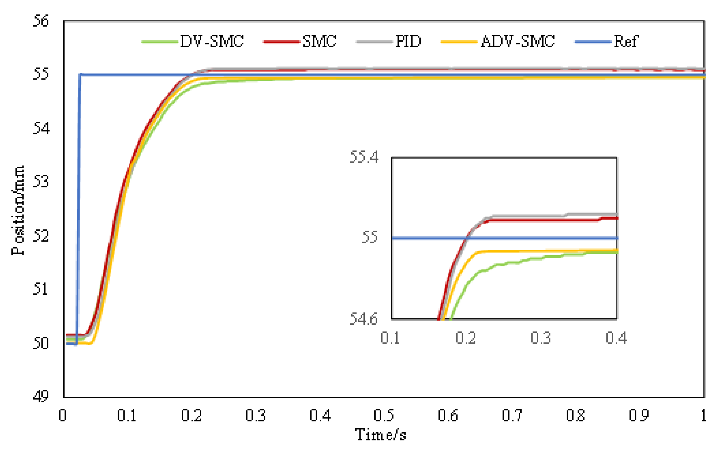
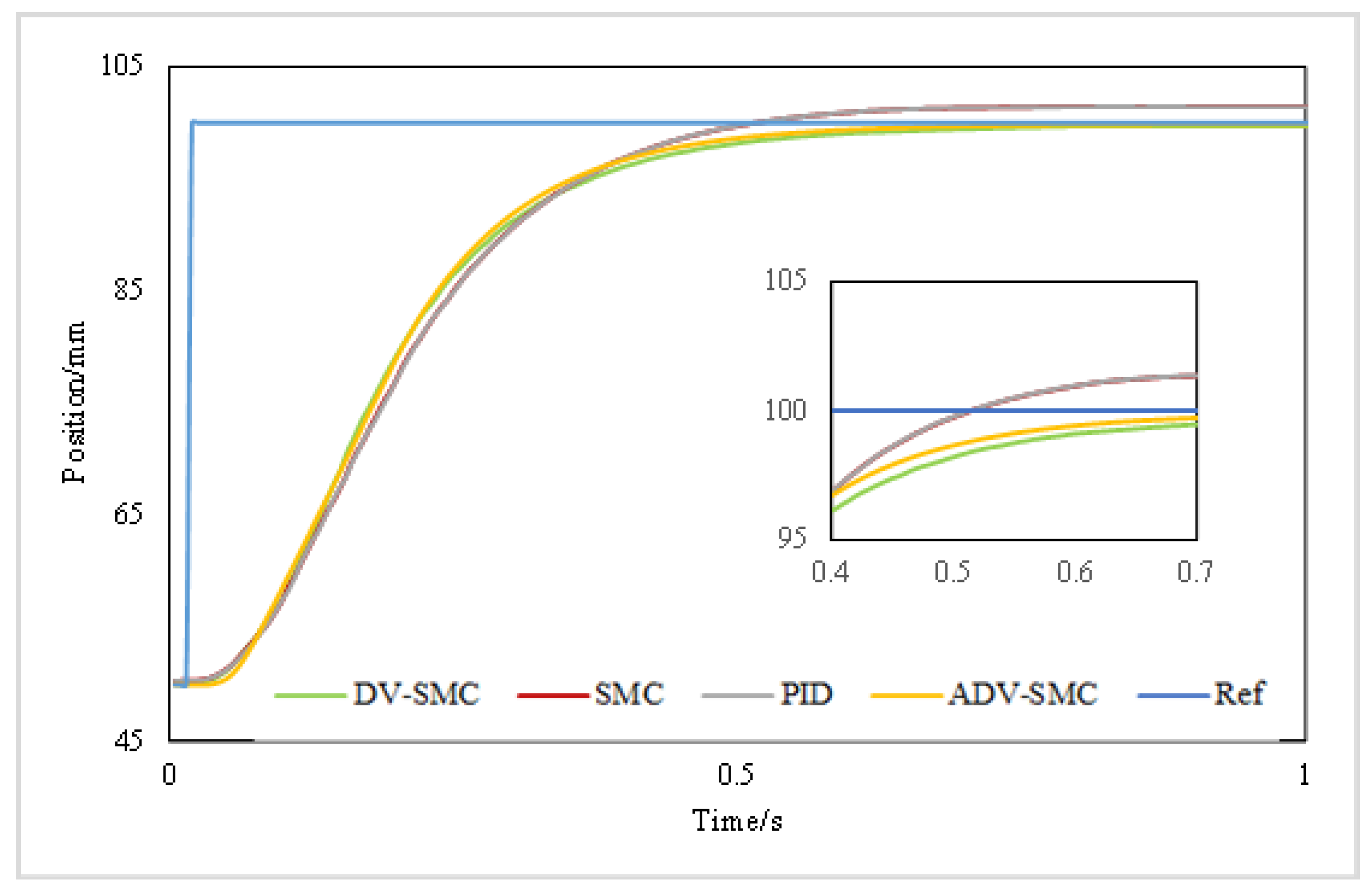
	5 mm		50 mm
	ST/s	OS	ST/s	OS
PID	1+	0.024	1.8+	0.029
SMC	0.925	0.022	1.8+	0.029
DV-SMC	0.285	0	1.63	0
ADV-SMC	0.205	0	1.03	0

, the settling time is effectively cut down with the use of the ADV-SMC strategy. For the 5 mm step input, PID fails to reach the reference within 1 s, while SMC obtains a settling time of 0.925 s. Both PID and classical SMC generate an OS of 0.024 mm. Compared to SMC, our model reduces the settling time by 0.72 s. Furthermore, the use of parametric adaptation in ADV-SMC gives a slight improvement in response speed compared to DV-SMC. A similar outcome is the responses to 50 mm step input. The ESOs in these two controllers facilitate the control by estimating the external disturbance. In addition, by implementing the variable damping sliding mode surface, the overshoot is suppressed, thereby eliminating the contradiction of system rapidity and stability. Notably, the settling time of ADV-SMC is better that of DV-SMC by 0.08 s in the 5 mm step input test. The main reason for this is that the ARC scheme is capable of estimating the system parameters to further enhance the system rapidity. As such, our controller obtained the best and most consistent results in both evaluation settings.

PID: three-loop PID control; SMC: SMC with double-loop PID control; DV-SMC: DV-SMC with double-loop PID control; ADV-SMC: ADV-SMC with double-loop PID control (same for Figure 6 and Figure 7).

Figure 7 presents the results of tracking $x_d=0.04\sin (\pi t)[1-\exp (-t^3)]$ with the four controllers. ADV-SMC is still the best-performing method in this test. According to Figure 7, there is a considerable gap between ADV-SMC and other controllers on tracking errors. Specifically, the maximum tracking errors are as follows: 2.4 × 10⁻³ m for PID, 3.0 × 10⁻⁴ m for SMC, 3.6 × 10⁻⁴ m for DV-SMC, and 1.2 × 10⁻⁴ m for ADV-SMC. These performance gaps range from 2.3 × 10⁻³ m (PID) to 1.7 × 10⁻⁴ m (SMC), which are significant (Table 2). With the same robust gain parameters and within the last period, the maximum position tracking errors for ADV-SMC, DV-SMC, and SMC are 0.2, 0.4, and 0.3 mm, respectively. It is worth noting that the tracking accuracy of DV-SMC does not exceed that of SMC. A possible explanation is that the first and second derivatives of x_d are set as 0 to suppress the overshoot in DV-SMC, which weakens the capability in steady-state response. In this case, removing the feedforward compensation term from basic SMC has an impact on the sinusoidal tracking accuracy and leads to the accumulating of tracking errors.

As presented in Figure 7a, the proposed ADV-SMC has comparable tracking performance to the DV-SMC during the initial stage due to the limited effect of parametric adaption within such a short time. Subsequently, related parameters are regulated and reduce the initial tracking error. Starting from the second period, the tracking error of ADV-SMC tends to converge, and the tracking outcome improves gradually, which results from the convergence of the adapted parameters. It can be observed that the tracking of ADV-SMC continuously outperforms that of SMC from the third period to the end of testing. In addition, Figure 7b exhibits the convergence of the parametric estimation of ADV-SMC. While the tracking error of ADV-SMC starts to converge, the adaptive parameters also tend to stabilize. We see that θ1 and θ3 reach the maximum and minimum values as a result of the nonlinear projection, whereas θ2 varies periodically within bounded ranges. During this phase, the tracking error significantly drops, which confirms that the parametric adaptation relieves some of the burden of the robust items and contributes to high-precision tracking.

Additionally, Figure 7c shows the corresponding control outputs of the four control strategies. One can observe that the output of PID control stays continuous, especially at the speed reversal point of the piston rod. Considering the impact of the dead zone, the tracking error is enlarged in this test. In addition to PID control, there is a spike in output of the other three control strategies. These spikes result from the robust items, which drive the EHA to cross the dead zone in a manner that inhibits the friction. Moreover, the ARC principle in ADV-SMC further enhances overcoming the dead zone via parametric estimation. As such, it is reasonable to expect better robustness against system uncertainties and disturbances and thus better controlling performance, as is the case.

In order to clarify the effectiveness of our controller, position tracking data of the last two periods were selected for further analysis. Three indicators—average error, maximum error, and variance of error—were derived to characterize the working performance of four control strategies (see

Table 3. Tracking errors of sinusoidal input.

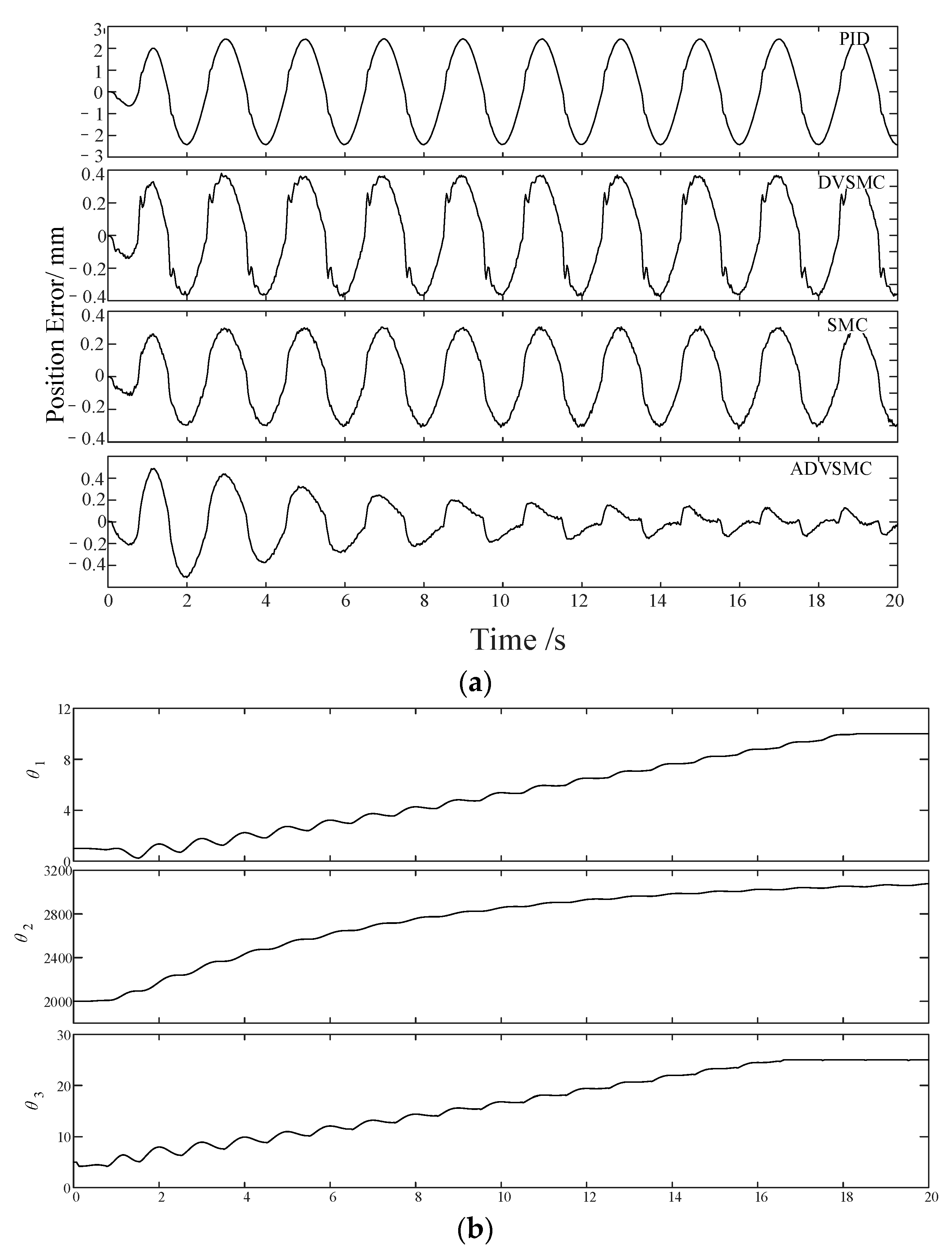
Error	Average	Maximum	Variance
PID	0.001589	0.002421	5.17 × 10−7
DV-SMC	0.000252	0.000362	1.02 × 10−8
SMC	0.000205	0.000297	6.64 × 10−9
ADV-SMC	4.42 × 10−5	0.000123	1.74 × 10−9

). We noted that PID obtained the worst error evaluation outcomes. Errors of SMC had a marginal improvement over those of DV-SMC. Clearly, our model is a better alternative to the other controllers, which had 21.5, 41.4, and 26.2% SMC, respectively.

5. Conclusions

This work extends our previous study [20] to resolve the parametric uncertainty of the DV-SMC strategy in the EHA control task. In essence, an ADV-SMController is established, which is composed of a variable-damping SMC model against system uncertainties, an ESO to observe external disturbance, and an ARC law for parametric estimation. Experimental results indicate that the proposed ADV-SMC strategy is the best alternative for EHA control compared to the state-of-the-art control methods. In one sense, the parametric uncertainties in EHA are effectively captured and compensated by employing an adaptive control law in controlling. In another sense, the parametric adaption further facilitates improved tracking accuracy and speed. In contrast with the DV-SMC, our controller further eliminates the tracking error that results from the absence of feedforward items and relieves the burden of the robust items. Nevertheless, although an improved sign function is applied for the suppression of chattering, the elimination of chattering is not achieved fundamentally, which leads to future research.

References

- Maré, J.-C.; Fu, J. Review on signal-by-wire and power-by-wire actuation for more electric aircraft. Chin. J. Aeronaut. 2017, 30, 857–870. [Google Scholar] [CrossRef]
- Alle, N.; Hiremath, S.S.; Makaram, S.; Subramaniam, K.; Talukdar, A. Review on electro hydrostatic actuator for flight control. Int. J. Fluid Power 2016, 17, 125–145. [Google Scholar] [CrossRef]
- Shang, Y.; Li, X.; Qian, H.; Wu, S.; Pan, Q.; Huang, L.; Jiao, Z. A Novel Electro Hydrostatic Actuator System With Energy Recovery Module for More Electric Aircraft. IEEE Trans. Ind. Electron. 2020, 67, 2991–2999. [Google Scholar] [CrossRef]
- Marco, V.; Marco, T.; Giuseppe, F.; Luca, C. Electromechanical Actuator for Helicopter Rotor Damper Application. IEEE Trans. Ind. Appl. 2014, 50, 1007–1014. [Google Scholar]
- Qiao, G.; Liu, G.; Shi, Z.; Wang, Y.; Ma, S.; Lim, T.C. A review of electromechanical actuators for More/All Electric aircraft systems. Proc. Inst. Mech. Eng. Part C J. Mech. Eng. Sci. Nov. 2017, 232, 4128–4151. [Google Scholar] [CrossRef]
- Bossche, D. The A380 flight control electro-hydrostatic actuators, achievements and lessons learnt. In Proceedings of the 25th International Congress of the Aeronautical Sciences, Hamburg, Germany, 3–8 September 2006; pp. 1–8. [Google Scholar]
- Qi, H.T.; Fu, Y.L.; Qi, X.Y.; Lang, Y. Architecture Optimization of More Electric Aircraft Actuation System. Chin. J. Aeronaut. 2011, 24, 506–513. [Google Scholar] [CrossRef]
- MOOG Inc. Electro Hydrostatic Actuators; MOOG Inc.: Salt Lake City, UT, USA, 2014. [Google Scholar]
- Zhao, J.A.; Fu, Y.L.; Ma, J.M.; Fu, J.; Chao, Q.; Wang, Y. Review of cylinder block/valve plate interface in axial piston pumps: Theoretical models, experimental investigations, and optimal design. Chin. J. Aeronaut. 2021, 34, 111–134. [Google Scholar] [CrossRef]
- Shea, A.; Jahns, T.M. Hardware integration for an integrated modular motor drive including distributed control. In Proceedings of the 2014 IEEE Energy Conversion Congress and Exposition (ECCE), Pittsburgh, PA, USA, 14–18 September 2014; pp. 4881–4887. [Google Scholar]
- Wang, J.; Li, Y.; Han, Y. Integrated modular motor drive design with GaN power FETs. IEEE Trans. Ind. Appl. 2015, 51, 3198–3207. [Google Scholar] [CrossRef]
- Yang, Y.S.; Niu, W.Q.; Zhao, J. Design and Numerical Study of Electro-Hydrostatic Actuator. J. Phys. Conf. Ser. 2019, 012088, 1–9. [Google Scholar] [CrossRef]
- Ren, G.; Esfandiari, M.; Song, J.; Sepehri, N. Position Control of an Electro-hydrostatic Actuator with Tolerance to Internal Leakage. IEEE Trans. Control Syst. Technol. 2016, 24, 2224–2232. [Google Scholar] [CrossRef]
- Zhang, H.; Liu, X.; Wang, J.; Karimi, H.R. Robust H∞ Sliding mode control with pole placement for a fluid power electrohydraulic actuator (EHA) system. Int. J. Adv. Manuf. Technol. 2014, 73, 1095–1104. [Google Scholar] [CrossRef]
- Wang, C.; Quan, L.; Jiao, Z.; Zhang, S. Nonlinear Adaptive Control of Hydraulic System With Observing and Compensating Mismatching Uncertainties. IEEE Trans. Control Syst. Technol. 2018, 26, 927–938. [Google Scholar] [CrossRef]
- Yao, Z.K.; Yao, J.Y.; Yao, F.Y. Model reference adaptive tracking control for hydraulic servo systems with nonlinear neural-networks. ISA Trans. 2019, 100, 396–404. [Google Scholar] [CrossRef] [PubMed]
- Wang, M.K.; Fu, Y.L.; Zhao, J.A. A Novel Cascade Control Based on Damp Variable Sliding Mode Control for an Electro-hydrostatic Actuator. J. Beijing Univ. Aeronaut. Astronaut. 2020. (In Chinese) [Google Scholar] [CrossRef]
- Yang, R.R.; Fu, Y.L.; Zhang, G.L. A Novel Sliding Mode Control Framework for Electrohydrostatic Actuator. Math. Probl. Eng. 2018, 7159891. [Google Scholar] [CrossRef]
- Ataklti, E.A.; Fu, Y.L. Sliding mode control of electro-hydrostatic actuator based on extended state observer. In Proceedings of the 29th Chinese Control And Decision Conference, Chongqing, China, 28–30 May 2017; pp. 758–763. [Google Scholar]
- Wang, M.; Wang, Y.; Yang, R.; Fu, Y.; Zhu, D. A Sliding Mode Control Strategy for an ElectroHydrostatic Actuator with Damping Variable Sliding Surface. Actuators 2020, 10, 3. [Google Scholar] [CrossRef]
- Ali, S.A.; Christen, A.; Begg, S.; Langlois, N. Continuous–discrete time-observer design for state and disturbance estimation of electrohydraulic actuator systems. IEEE Trans. Ind. Electron. 2016, 63, 4314–4324. [Google Scholar] [CrossRef]
- Throne, D.; Martinez, F.; Marguire, R.; Arens, D. Integrated Motor/Drive Technology with Rockwell Connectivity. Rexroth, Bosch Group, Lohr am Main, Germany, Tech. Rep. Available online: http://www.cmafh.com/enewsletter/PDFs/IntegratedMotorDrives.pdf (accessed on 17 April 2021).
- Kim, H.-J.; Park, H.-S.; Kim, J.-M. Expansion of Operating Speed Range of High-Speed BLDC Motor Using Hybrid PWM Switching Method Considering Dead Time. Energies 2020, 13, 5212. [Google Scholar] [CrossRef]
- Berri, P.C.; Vedova, M.D.L.D.; Maggiore, P. A Simplified Monitor Model for EMA Prognostics. Matec Web Conf. 2018, 233, 00016. [Google Scholar] [CrossRef][Green Version]
- Yao, B.; Bu, F.; Reedy, J.; Chiu, G.C. Adaptive Robust Motion Control of Single-Rod Hydraulic Actuators: Theory and Experiments. IEEE/ASME Trans. Mechatron. 2000, 5, 79–91. [Google Scholar]