Abstract
Twisted coiled actuators (TCAs) are a type of soft actuator made from polymer fibres such as nylon sewing thread. As they provide motion in a compact, lightweight, and flexible package, they provide a solution to the actuation of wearable mechatronic devices for motion assistance. Their limitation is that they provide low total force, requiring them to actuate in parallel with multiple units. Previous literature has shown that the force and stroke production can be improved by incorporating them into fabric meshes. A fabric mesh could also improve the contraction efficiency, strain rate, and user comfort. Therefore, this study focused on measuring these performance metrics for a set of TCAs embedded into a woven fabric mesh. The experimental results show that the stroke of the actuators scaled linearly with the number of activated TCAs, achieving a maximum applied force of 11.28 N, a maximum stroke of 12.23%, and an efficiency of 1.8%. Additionally, two control methods were developed and evaluated, resulting in low overshoot and steady-state error. These results indicate that the designed actuators are viable for use in wearable mechatronic devices, since they can scale to meet different requirements, while being able to be accurately controlled with minimal additional components.
1. Introduction
Stroke is one of the leading causes of death and disability in the world, with the WHO projecting a total of 61 million disability-adjusted life years lost to stroke worldwide in 2020 [1]. Stroke often impairs motor functions, with arm paresis in particular being common among patients [2]. In order to return mobility to such patients, repetitive task training is often used, with favourable results; however, access to such therapy is often limited by the cost and availability of trained therapists [3]. To address this, wearable robotic devices have been shown to be effective methods of implementing this therapy, by aiding motor control recovery after stroke events [4]. When used by therapists, they reduce the required number of contact hours with patients, and in some cases, even allow non-therapist operators to control them after initial setup [5]. If the convenience and portability of wearable devices could be increased, they could even be used at home, which has been shown to increase patient adherence to exercise [6], would remove accessibility barriers, and allow for continued use during service disruptions, such as during pandemics or other disasters.
Increased portability and convenience could be achieved by replacing electromagnetic motors in such devices, which are inherently cylindrical and rigid, with a flexible artificial muscle-like actuator system embedded into a flexible, textile-based wearable device. Nylon 6,6 twisted coiled actuators (TCAs) are a smart material actuator that has higher power to weight output, larger force generation, larger stroke, and more linear behaviour with less hysteresis when compared to other smart material actuators [7]. When heat is applied to a TCA fibre, it contracts more than 20% of its initial length, and exerts stresses greater than 35 MPa, which is 100 times greater than biological muscle fibres [8]. This can be done by passing an electric current through a conductive heating element bound with the constituent twisted nylon, such as silver paint, to make the actuators electrically controllable [9]. While TCAs have many desirable characteristics, they do have some drawbacks: they have low efficiency, low gross force per unit fibre, and tend to have a slow response time, especially in relaxation compared to contraction [10], which has been addressed previously through the use of pressurised air to facilitate rapid cooling times [11]. Their shortcomings affect their ability to be adopted in clinical and commercial devices, but there are promising methods of overcoming these issues.
Currently, in the literature, it has been found that incorporating smart material actuators into fabric meshes can improve stroke and force production compared to other multi-fibre actuators [12], which, if the same holds true for TCAs, could be a way of improving their force production capabilities. Doing so also has the possibility of increasing the efficiency of the actuators by increasing the thermal insulation surrounding them, reducing the amount of waste heat generated during the contraction phase. To further improve performance, multi-fibre bi-pennate structures mimicking human muscle could be used as the base structure for a woven actuating module. This structure arranges opposing pairs of artificial muscles along a central tendon at an acute angle to let them work together without interfering with one another, similar to how biological muscle fibres are arranged in the human body [13]. Multiple TCAs working in tandem would increase the maximum force production of the unit, as seen in other examples of biomimetic structures incorporating TCAs [14], with a structure that also has the added benefit of architectural-based velocity gearing [15]. This feature innately dampens disturbances, increasing the safety for the user over normal compliant actuators. This paper proposes to make use of a woven fabric mesh with an embedded pennate structure comprised of TCAs to create a viable actuation module for therapeutic wearable robotic devices, characterise its stroke and force production, and implement control schemes to control the force output of the actuating module.
2. Actuator Characterisation
2.1. Materials and Methods
In order to meet these objectives, a series of experiments were conducted. First, the stroke and force production capabilities of the actuator were characterised in an isotonic and isometric configuration, respectively, with the efficiency of the actuator being calculated for the isotonic contraction experiment. Next, the performance of the actuator at elevated contraction speeds was investigated, looking at how it performed with a 2 s contraction time (chosen based on therapy frequency requirements found by Polygerinos et al. [16]) and at its minimum possible contraction period, while still achieving a full range of motion. The final set of experiments explored the performance of the actuator when attempting to produce a constant force setpoint when controlled by both a proportional-integrative-derivative (PID) controller and a 2-degree-of-freedom (DOF) feedforward-feedback composite controller.
2.1.1. TCA Fabrication and Training
Using a method derived from Cho et al. [17], to construct the TCAs, a 2.5 m length of silver coated nylon thread (Shieldex 4-ply Coated Nylon Thread 260151023534) was attached at one end to a DC motor. The other was attached to 175 g of calibration weights, to keep the thread taut while the motor spun to twist the thread. The DC motor spun the thread until it first became coiled, then supercoiled, which occurred when the thread completely coiled on itself twice, significantly shortening and changing the width of the thread structure. The supercoiled thread was then clamped with non-insulated quick-disconnect terminals (Electerm BB2-MQ1) in 100 mm intervals, measured from the base of the terminals. These intervals were selected to be free of snags, runs, and other irregularities. Excess material was then trimmed so that the terminals were the endpoints of the TCAs.
After creating the TCAs, they needed to be trained in order to contract when heated. To do this, an untrained TCA was attached to a rigid structure, with a metal hook at one end and a free-hanging 50 g calibration weight at the other, to keep it taut. The TCA was then attached via alligator clips to a DC power supply (BK Precision 1671A), and 0.8 A of current was applied at 3.6 V, giving a total initial power delivery value of 2.88 W. This heated the actuator through Joule heating, dissipating the power losses in the actuator as heat to raise its temperature. The temperature of the actuator was measured using a thermocouple (Agilent U1272A (with Thermocouple Attachment)). Once the TCA reached 120 °C, the DC power supply was shut off to prevent overheating and damaging the actuator, and begin cooling the actuator. The TCA was allowed to cool to room temperature, measured using readings from the thermocouple. This heating and cooling cycle was repeated five times per TCA, after which the TCA was considered trained and able to contract with the application of Joule heating. The difference between an untrained and trained TCA can be seen in Figure 1.
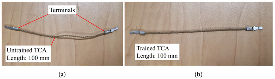
Figure 1.
(a) Untrained twisted coiled actuator (TCA). (b) Trained TCA.
2.1.2. Actuator Fabrication
The full actuation module was constructed by stringing a number of pairs of TCAs (dependent on experiment) between rigid side tendons and a rigid central tendon, with a small amount of tension applied to keep the TCAs taut. To keep the TCAs attached, pins were embedded within the tendons and the TCAs were slid over them. Then, purpose-built 3D printed caps were slid over the pins in order to keep the TCAs attached while allowing for rotation. After doing this, thermocouples were fed through retaining slots, which were constructed as part of the pin caps, and attached to the TCAs at a distance of 2 cm from the end of the thermocouple guide. They were tied to the TCAs with nylon thread underneath their weld bead, snugly affixing them to the actuating fibres (see Figure 2). Thermal paste (Halzniye 510) was then applied liberally to eliminate air gaps between the thermocouples and the TCAs, to improve the thermal conductivity and electrical insulation between the two components. Once the thermal paste had been applied, the actuator was woven using 100% nylon 18 weight yarn (Annie’s Catalog 1005019) using a standard over–under manual weaving technique. This was done by attaching the yarn to a weaving needle, and manually passing it through each TCA, passing the yarn over, then under, each successive TCA. The needle was then turned around, and passed through the TCAs again in the opposite direction, going over each TCA where it had gone under the previous pass, and vice versa, to create a loop encompassing each TCA. Each pass, the yarn loops were compressed against one another to make the weave as tight as possible. This weaving procedure continued until the thermocouples attached to the TCAs had been covered by a minimum of three loops, and then was repeated on the other side to complete the mesh. An actuator in the process of being woven can be seen in Figure 3. Upon completion of both sides, the side tendons were adjusted to ensure a 45° pennation angle between the central tendon and the TCA fibres, after which the actuator was considered fabricated and ready for experimentation, as seen in Figure 4.
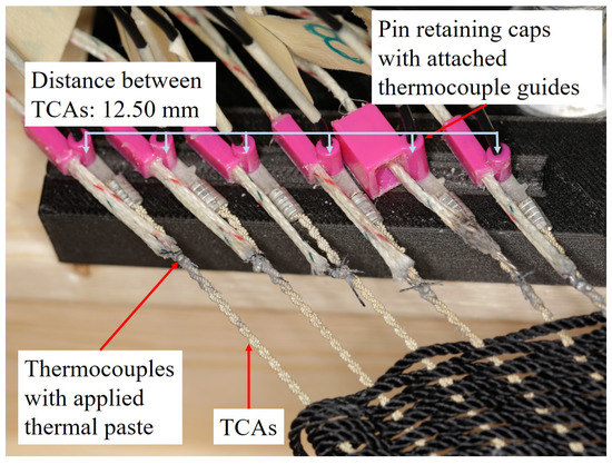
Figure 2.
Thermocouples after having been attached to the TCAs, with thermal paste applied.
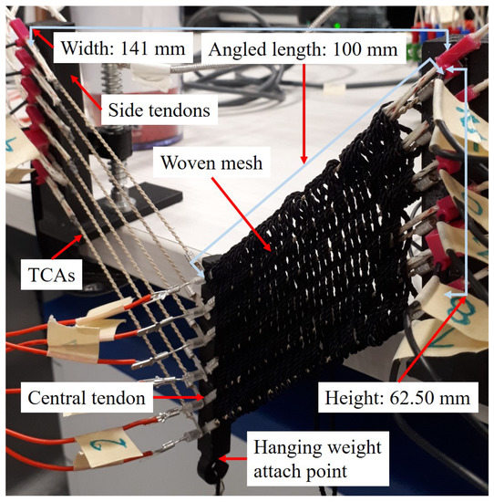
Figure 3.
Actuator in the process of being woven. The right side has been completely woven, while the left has yet to be woven.
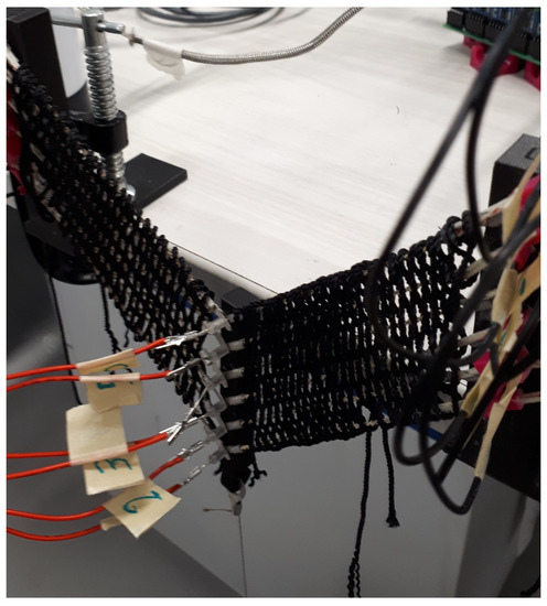
Figure 4.
Actuator configuration for the stroke characterisation experiment.
2.1.3. Actuator Characterisation
To characterise the stroke production of the actuator, ten actuators were constructed, with six constituent pairs of newly fabricated and trained TCAs, following the method detailed above. They were placed in a vertical configuration on a levelled lab bench, such that a weight could be freely hung from the central tendon, as seen in Figure 4. After doing so, 1.2 kg of calibration weights were hung from the hook of the central tendon and an IR distance sensor (SHARP GP2Y0A51SK0F) was affixed to the bottom of the weights, such that it was pointed at a controlled reflectivity surface on the ground. After adjusting the actuator and making sure a 45° pennation angle was still maintained, the experiment commenced. The number of pairs of TCAs being heated, or activation levels, were iteratively tested to determine its stroke production capacity. A pair of TCAs was chosen randomly to designate it as “activated”, and it was supplied with a maximum of 30 W (10 V at 3 A) of power by a programmable DC power supply (Rigol DP811). Transistors (Vishay Silconix SI3900DV) controlled this supply, being kept open to allow the activated TCAs to heat until they both reached a temperature of 80 °C, as read by the attached thermocouples. If one TCA achieved this temperature before the other, its power was cut off by closing its transistor until its temperature went below 80 °C, when its transistor was opened again until it went over 80 °C once more. This oscillation continued until both active TCAs reached the 80 °C threshold.
Once they achieved this temperature, the power was cut off to allow them to cool to a temperature of 30 °C. After cooling to this point, the trial was considered complete, and the process would begin again with another randomly selected pair of TCAs. Throughout the trial, the TCA temperatures, power consumed (Texas Instruments INA219B), the distance of the weights from the ground, and time elapsed were logged using a microcontroller (Espressif ESP32) at a sampling rate of 0.11 s, with the limiting speed factor being the communications between the thermocouple amplifiers (Maxim IC MAX6675) and the microcontroller. This was repeated for a total of five trials for that actuator at that activation level.
After this set of trials was finished, the power available for the actuator was increased by 10 W by increasing the available current by 1 A. The activation level was increased to two pairs of active TCAs, and five trials were completed following the same procedure as before. This process was repeated, increasing the number of activated pairs by one every five trials, and increasing the power available to the actuator by 10 W by increasing the available current by 1 A, until all of the activation levels (six in total) were completed. In summary, five trials were completed per activation level, for a total of 30 trials per actuator. After these were complete, the actuator was disassembled and a new actuator was made with a new set of TCAs, and evaluated in the same way. This was repeated until ten actuators had been tested, giving a total of 50 trials per activation level.
The force characterisation experiment was performed in a similar manner on actuation modules comprised of six pairs of TCAs, using the same grouping of TCAs as in the stroke characterisation experiment. Instead of constructing the modules in a vertical configuration, they were constructed horizontally in a purpose-built rigid structure, and attached to a load cell (Bolson Tech 5 kg load cell with a XFW-HX711 amplifier) with the hook on the central tendon, as seen in Figure 5. After the construction of the actuation modules, the side tendons were adjusted to ensure a 45° pennation angle once more, and the same heating and cooling procedure described above was applied to the module. Each of the six activation levels were tested a total of five times per actuator, measuring the temperature of the active TCAs, their power consumption, the force exerted by the module on the load cell, and the time elapsed at a sampling interval of 0.11 s. The results were recorded once more on an ESP32 microcontroller. A total of ten actuators were tested this way, giving a total of 50 trials per activation level.
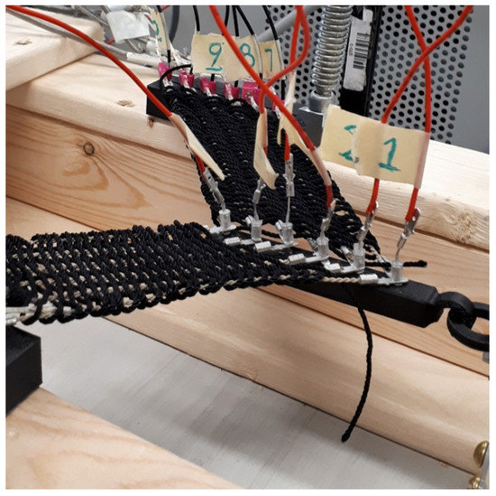
Figure 5.
Actuator configuration for the force characterisation experiment.
2.1.4. Contraction Period
After characterizing the performance of the actuators at a slow speed, additional experiments were performed to determine how they behaved at elevated contraction speeds, with the goal of determining their best possible response time. Tests similar to those used to characterise the stroke of the actuation module were performed with this purpose. The number of constituent pairs of TCAs in the modules tested was reduced from six to three, seen in Figure 6, but were otherwise fabricated as in the previous experiments in a vertical configuration, so that the isotonic stroke could be measured as in the stroke characterisation experiment. The power supplied to the actuator was set to the maximum possible given the electrical transmission components used, giving a supply of 80 W per active pair of TCAs at 20 V and 4 A. This gave a maximum of 240 W supplied to the actuator when all pairs were activated. The weight hung from the central tendon was reduced to 600 g, to account for the halving of the number of active pairs of TCAs.
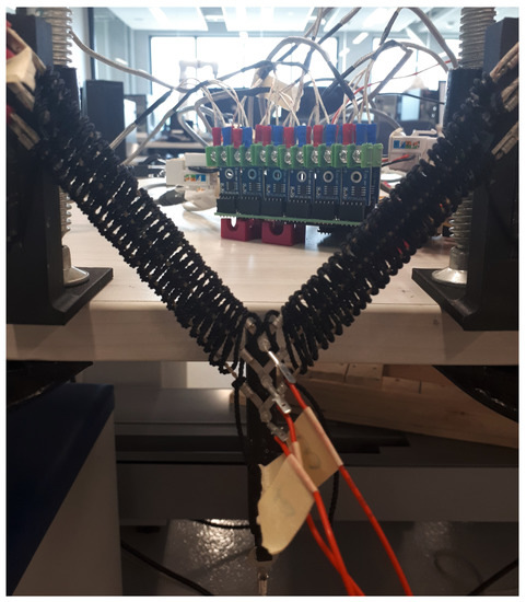
Figure 6.
Actuator configuration for the contraction period characterisation experiments.
After the actuating module was set up, the TCAs were operated on in a similar trial progression as in the stroke characterisation experiment, with two sets of tests being completed, with one having a variation in its heating procedure. Rather than attempting to achieve a target temperature of 80 °C, the active TCAs were heated for a set interval of 2 s. This was done to measure the stroke production capabilities of the actuator at a constant elevated contraction speed. This experiment will be referred to as the constant contraction period experiment. The second test was performed according to the same procedure as in the stroke characterisation experiment, being heated until an average temperature of 80 °C was achieved before being allowed to cool to 30 °C for each trial performed. This was done in order to determine the minimum contraction period that the actuator was capable of achieving in its current configuration. This will be referred to as the minimum contraction period experiment. Throughout each trial, for both tests, the time elapsed, stroke, and temperature were recorded. The trial progressions were the same as in the stroke characterisation experiment, with each activation level being tested five times per actuator per test. Six actuators were tested, giving 30 trials per active level in total for each test.
2.1.5. Analytical Methods
In order to determine the significance of effects between different activation levels and the constructed actuation module, repeated measures one-way ANOVAs were conducted. The within-subjects factor being tested was the differences between different activation levels (e.g., force and stroke produced, and heating time), while the between-subjects factors being tested were the different fabricated actuators, to determine the consistency of results between different modules. Where applicable, the different control schemes were also a between-subjects factor that was tested, to determine the differences in performance between the two controllers. These were all completed with an value of 0.05 and a value of 0.80, to achieve desired certainty thresholds. Bonferroni corrections were applied to address repeated independent comparisons. Due to the comparisons between different time values, Kruskal–Wallis analyses were also conducted to determine the differences between different groupings of trials (e.g., time constant and peak time differences between the responses of different controllers). Confidence intervals were also calculated using the standard confidence interval equation:
where is the mean of the dataset, is the standard deviation, n is the number of samples, and Z is the z score associated with the desired certainty level. For a certainty of 95%, the Z value is set to 1.96. All analyses were performed with the assistance of IBM SPSS Statistics, Version 27.
2.2. Results
2.2.1. Actuator Characterisation
After performing all of the trials for each activation level of each actuator in both the stroke and force characterisation, the temperature of each active TCA at each time point was averaged to find the mean active temperature of the actuator, and the initial distance and force produced was subtracted from each subsequent point in their respective points to obtain the additional values produced by the actuators. These results can be seen in Figure 7 for the stroke characterisation experiments, and Figure 8 for the force characterisation experiments. Once this was done, the trial was then split into two phases: the actuator in contraction, and the actuator in relaxation. These were separated by finding the time point at which the average temperature of the of the active TCAs began to decrease, while their total power consumption was zero. Afterwards, the maximum stroke and force produced by the actuation modules were calculated for each trial when in its contractive phase, to determine their maximum production capabilities. Having found the contractive capabilities of the actuators, confidence intervals were constructed from the maximum production values, and a linear regression was applied to their mean values to determine their linearity. These regressions can be seen in Figure 9.
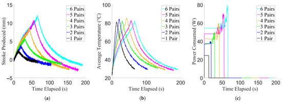
Figure 7.
Results of the stroke characterisation experiment, showing data from example trials. For the purpose of clarity, example curves were used, due to low variance between trials. (a) Stroke production of the actuator. (b) Temperature achieved by the actuator. (c) Power consumed by the actuator.
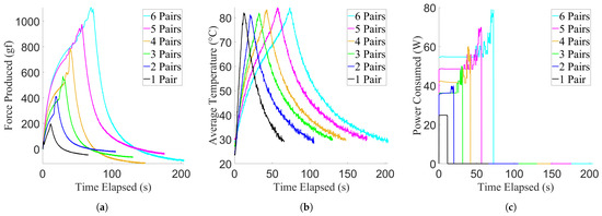
Figure 8.
Results of the force characterisation experiment, showing data from example trials. For the purpose of clarity, example curves were used due to low variance between trials. (a) Force production of the actuator. (b) Temperature achieved by the actuator. (c) Power consumed by the actuator.
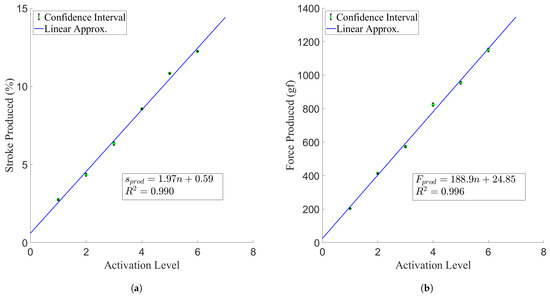
Figure 9.
Maximum actuator production per active pairs of TCAs, with overlaid linear regressions. The variable n denotes the number of activated pairs of TCAs. (a) Stroke production results. (b) Force production results.
The contraction results were then used to perform a univariate regression between temperature and the stroke or force produced by the actuator. The data were prepared by separating the contraction data from the relaxation data for each trial, and constructing a dataset for each activation level for each mode of production consisting of all of the paired values in that experiment. After this preparation, the regression was performed with temperature being the independent variable and stroke or force being the dependent variable. The polyfit function was used in the scripting language MATLAB. The degree of the regressed polynomial was tested iteratively from a degree of one to ten in order to find the degree that minimised the average root mean square error across all activation levels for each type of regression. From this procedure, it was found that a degree of one could be used to model the relationship between temperature and stroke, with minimal error and without overfitting, while a degree of five was chosen to model the relationship between temperature and force. The form of the one degree temperature–stroke regression can be seen in Equation (2), and the form of the degree five temperature–force regression can be seen in Equation (3). These equations give the general form of their respective relationships, with and referring to the stroke and force produced by the actuator, respectively, T referring to the temperature of the actuator in degrees celsius, and – referring to the polynomial coefficients that comprise the polynomial regressions. The coefficients for the regressed functions for each activation level from one to three can be found in Table 1 and Table 2 for stroke and force respectively. How those regressions fit for the temperature–stroke and temperature–force relationships can be seen in Figure 10 and Figure 11, respectively. The regressed force functions were used in Section 3.1 in order to construct the force controllers.

Table 1.
Regressed temperature–stroke relationships, as described in Equation (2), by activation level.
Table 2.
Regressed temperature–force relationships, as described in Equation (3), by activation level.
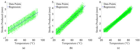
Figure 10.
Regressed temperature–stroke relationships overlaid over experimental data, separated by activation level. (a) One activated pair. (b) Two activated pairs. (c) Three activated pairs.
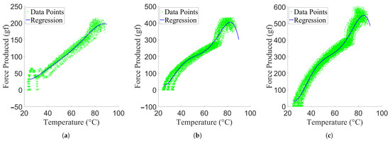
Figure 11.
Regressed temperature–force relationships overlaid over experimental data, separated by activation level. (a) One activated pair. (b) Two activated pairs. (c) Three activated pairs.
Looking at the results of the repeated measures one-way ANOVA performed for within-subject factors, a null-hypothesis can be rejected for each of the activation levels in contraction for stroke and force produced ( for all comparisons). This indicates that each additional pair of TCAs produced statistically significant differences in stroke and force production. Comparing the between-subject factors, it was found that there were no statistically significant differences between different actuation modules operating at the same activation level in terms of either the stroke or force produced in contraction ( and , respectively), indicating that the production at each activation level is similar across different fabricated instances of the actuation module, denoting consistency in contraction.
However, it should be noted that the actuators did not perform the same in contraction and relaxation. From Figure 7 and Figure 8 it can be seen that slack was introduced into the actuators during the relaxation phase, with both the force and stroke produced decreasing below the origin point. This is indicative of non-linearities present in the stroke and force production of the system due to hysteresis. To quantify this effect, the average stroke and force production at each temperature point for each activation level was found and averaged across each trial, to give one average temperature–stroke and temperature–force curve for each activation level. These curves can be seen in Figure 12.
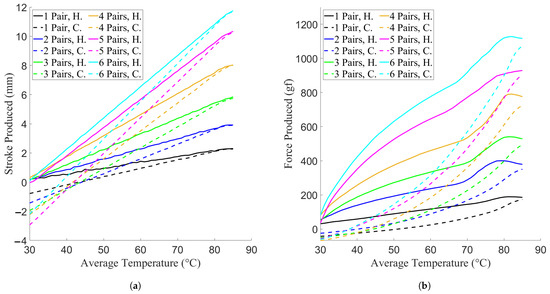
Figure 12.
Average hysteresis at each activation level during the characterisation experiments. The abbreviation “H.” denotes the production of the actuator while it is heating, and the abbreviation “C.” denotes the production of the actuator while it is cooling. (a) Stroke production hysteresis curves. (b) Force production hysteresis curves.
After doing so, the peak and root mean square (RMS) offset was calculated for each activation level for both stroke and force, which can be seen in Table 3 and Table 4 for stroke and force, respectfully. Looking at these values and curves, it can be seen that for each mode of production, the difference between the actuators’ production is inversely proportional to the achieved temperature; that is, the lower the temperature, the greater the difference in production.
Table 3.
Calculated peak and RMS hysteresis per activation level for the stroke characterisation experiment.
Table 4.
Calculated peak and RMS hysteresis per activation level for the force characterisation experiment.
2.2.2. Contraction Period
Similar to the characterisation results, after the data were collected, they were processed by averaging the temperature values for each TCA at each time point, and the initial distance was subtracted from further values to get the contractive stroke. The results of this can be seen in Figure 13 for the constant contraction period experiments and Figure 14 for the minimum contraction period experiments. The data were again split into contracting and relaxing phases, and the maximum temperature and stroke for each contractive phase was found. Similar again to the characterisation results, confidence intervals were constructed from the maximum production values, and linear regressions were applied to their mean values to determine their linearity. These regressions can be seen in Figure 15.
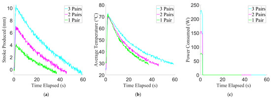
Figure 13.
Results of the constant contraction period experiment, showing data from example trials. For the purpose of clarity, example curves were used, due to low variance between trials. (a) Stroke production of the actuator. (b) Temperature achieved by the actuator. (c) Power consumed by the actuator.
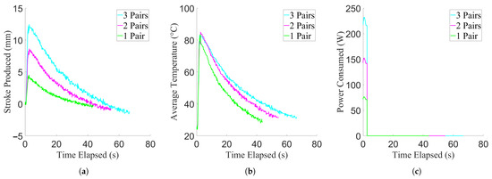
Figure 14.
Results of the minimum contraction period experiment, showing data from example trials. For the purpose of clarity, example curves were used due to low variance between trials. (a) Stroke production of the actuator. (b) Temperature achieved by the actuator. (c) Power consumed by the actuator.
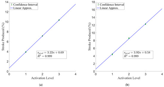
Figure 15.
Maximum stroke production per active pairs of TCAs, with overlaid linear regressions. The variable n denotes number of active pairs of TCAs. (a) Constant contraction period experiment. (b) Minimum contraction period experiment.
Similar to the characterisation experiments, from the results of repeated measures one-way ANOVA performed for within-subject factors, the null-hypothesis can be rejected ( for all comparisons) for each of the activation levels in terms of stroke produced in contraction for each of the contraction speeds investigated. When applied to the time required to reach 80 °C in the minimum contraction period experiment, it was found that there were no statistically significant differences between activation levels in the time required to reach the desired temperature ( for all comparisons). This was reaffirmed by the results of the Kruskal–Wallis testing done on the time values, which also found no statistically significant differences between activation levels ( for all comparisons). Comparing the between-subject factors, it was found that there were no statistically significant differences between different actuation modules operating at the same activation level, in terms of either stroke produced or time required. To achieve the desired temperature in the minimum contraction experiment ( for the constant period stroke comparisons, and and for the minimum contraction period stroke and contraction time comparisons, respectively). This further reinforces that there are minimal differences between different fabricated modules in terms of contractive performance.
2.2.3. Efficiency
In addition to characterising the contractive performance of the actuating modules, their efficiency was also investigated. The efficiency was calculated by finding the ratio between the electrical power consumed and the mechanical work output of the actuator when lifting a mass in an isotonic configuration. Due to the power draw of the actuator changing over time from the internal resistances of the TCAs changing as they heated [18], as well as fluctuation from the temperature control, the total energy consumed needed to be calculated. This was done by multiplying the power draw at each sensor reading by the time elapsed since the previous data point, and then summing each of these values over the course of a whole trial to get the total energy consumed. The mechanical energy output of the system in the same time period was found by multiplying the gravitational force exerted on the system (a combination of the masses, the sensor, and the sensor holster) by the maximum stroke of that trial. This work value was then divided by the total energy consumed to get the efficiency for that trial. Confidence intervals for these values, calculated from the stroke characterisation and contraction period experiments, can be seen in Figure 16.
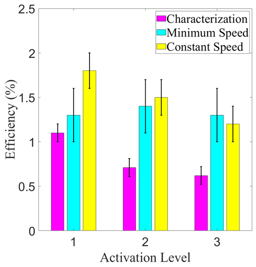
Figure 16.
Efficiency of the actuator during isotonic contractions compared to activation level, for the stroke characterisation experiment, minimum contraction period experiment, and constant contraction period experiment. Significance in differences not displayed due to inapplicability.
2.3. Discussion
2.3.1. Characterisation Experiments
From the value of the linear regressions performed (seen in Figure 9), it is apparent that the contraction of the actuator scales very linearly with the number of active pairs of TCAs, with a minimum value of 0.99 for the stroke regression. From the slopes of those two linear regressions, the stroke increased at a rate of 1.97 mm, or 1.97% stroke, per additional pair of active TCAs to a maximum value of 12.23%, and the force produced increased by 188.9 gf, or 1.85 N, per additional pair to a maximum value of 11.28 N. The maximum stroke production of the actuator is in line with other forms of artificial muscle actuators [19,20,21,22], and the additional force per active pair is comparable to [23,24,25] or better than [10,12,26] examples of actuating fibres and fabrics in the literature on a per-fibre basis. However, one has to consider that the TCAs are actuating at an angle, and thus are actually producing a greater stroke and force than those experienced at the end effector. By changing the initial pennation angle, one could feasibly increase both the stroke and force being applied by the actuator, improving on its performance to be beyond the examples found in the literature.
2.3.2. Contraction Period Experiments
Looking at the linearity of the results of the contraction period experiments, from the linear regressions performed (seen in Figure 15), the results were similar to the characterisation experiments, with the actuator scaling very linearly with the number of active pairs of TCAs at elevated contraction speeds, having a minimum value of 0.99 for each regression. From the maximum stroke production values, in the minimum contraction period experiment, the actuator was able to achieve similar stroke production values to the stroke characterisation experiment at significantly higher rates of contraction, seen in Table 5, with values ranging between 2.36 and 2.43 seconds to achieve the maximum contraction. This is a significant improvement over the actuation speeds of the characterisation experiment, and could be improved upon if the power supplied to the actuator was increased. In future endeavours, more robust power transmission components should be used to allow for this, as even greater actuation speeds would only result in more possible use cases for the actuator.
Table 5.
Average stroke and contraction period by activation level in the minimum contraction period experiment.
Now, looking at the results of the constant contraction period experiment, which did investigate elevated contraction speeds, it can be seen that decreasing the contraction period without scaling the power supplied to account for this decrease does not allow the actuation module to reach its full range of motion, reducing the stroke produced by the actuator compared to both the stroke characterisation experiment and the minimum contraction period experiment. The percent range of motion it was able to achieve compared to the minimum contraction period experiment can be seen in Table 6. As well, the heating time of the constant period experiment, expressed as a percentage of the minimum contraction period to achieve full range of motion, is shown at each level. From these results, it can be seen that, while the range of motion was restricted, it did not match the percent decrease in contraction period, which hints that increasing the contraction speed does not have a direct correlation to the range of motion lost.
Table 6.
Stroke and contraction period comparisons between the constant and minimum contraction period experiments, by activation level. All values expressed as percentages.
2.3.3. Efficiency
From the results of the efficiency investigation, it can be seen that efficiencies were fairly low, being between one and two percent. This is in line with values found in the literature [10], which report similar values [27]. Looking at the confidence intervals, however, the minimum contraction period experiment was able to improve its efficiency over the stroke characterisation experiment, and the constant contraction period experiment was able to improve its efficiency over the minimum contraction period experiment for all activation levels except the third. This indicates that increased actuation speeds increase the efficiency of the actuator, and future iterations with higher actuation speeds could see their efficiency improve beyond the values found in the literature. To accomplish this, however, more durable power transmission components and larger power supplies should be used to facilitate greater actuation speeds.
3. Force Control Implementation
3.1. Materials and Methods
After characterizing the stroke and force production of the actuator, as well as determining its performance at elevated contraction speeds, force control schemes were implemented to control the force output of the actuator. According to a literature review performed, 2 DOF feedforward–feedback controllers have been used to great effect in controlling single TCA fibres, improving accuracy [28], decreasing overshoot [29], improving recovery time [17], and minimizing oscillations about a setpoint [30]; hence, it was desirable to investigate their performance when used to control a multi-fibre pennate module. To provide a baseline comparison, a PID controller was also implemented. The controllers were constructed based on the force characterisation experiment results, which were used to construct a time domain relationship between force output and actuator temperature at each activation level. To find the relationship between actuator temperature and power, it was assumed that sources of thermal radiation had a negligible impact on the heating of the actuator, which, when applied to the general heating equation given in [31] and simplified, gives the following heating equation:
where T, , and are the current, initial, and ambient temperature in degrees Celsius, respectively, t is the time in seconds since the beginning of the application of power, P is the supplied power, is the thermal resistance of the actuator, and is the thermal time constant of the system. The average thermal resistance for each activation level of the actuator was calculated by dividing the difference between the maximum and minimum temperature of the actuator in the heating phase of its trial by its average power consumption [31], repeating for each trial of each activation level before being averaged across each level. The average time constants for each activation level were found as the time it took for the actuator to reach 63% of the difference between the initial and final temperature of the actuator in that trial [32], before being averaged across each activation level. The ambient temperature was assumed to be 25 °C, and the power input was set to 80 W per activated pair, as in the contraction period experiments. The calculated thermal constants can be seen in Table 7.
Table 7.
Thermal resistances and time constants of the system for each activation level, calculated from experimental data. With each additional pair of TCAs, the thermal resistance decreased due the additional surface area, which increased the active portion of the actuator’s heat loss capabilities.
After finding these values, a simulated experiment was performed using the calculated relationships. A simulated step input was created such that the power was held to 80 W per activated level until the temperature, calculated using Equation (4) with values from Table 7, was able to increase from 25 °C to 85 °C, and then set to zero until the temperature was able to cool to 30 °C, creating a simulated version of the temperature curve from the minimum contraction period experiment. Similarly, a simulated version of the temperature–force curves found in the force characterisation experiment were created for each activation level across the same temperature span. These sets of pairs of curves were then input into the System Identification Toolbox in MATLAB, which derived the power–temperature transfer functions and the temperature–force transfer functions for each activation level, as shown in Table 8.
Table 8.
Frequency domain transfer functions for the power–temperature relationships and the temperature–force relationships for each activation level of the actuator.
These transfer functions were then applied to a PID control loop in the simulation software Simulink, seen in Figure 17, so that the step response of the PID controller could be tuned. The chosen force values were based on the results of the force characterisation experiment, and can be seen in Table 9. In particular, special care was taken to minimize the overshoot and settling error of the controller, as errors of that nature would result in the misapplication of force to the user, which could cause harm. After tuning, the , , and coefficients were found to be the values found in Table 10.
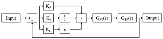
Figure 17.
Layout of the control flow for the PID controller.
Table 9.
Force setpoints used for controller tuning and testing purposes, based on the results of the force characterisation experiment, available in Figure 8.
Table 10.
Tuned PID coefficients.
After having tuned the PID controller, the step responses of the 2 DOF controllers were then simulated and tuned. The composition of the 2 DOF controller can be found in Figure 18. The same PID controllers as before were implemented for each activation level, leaving only the coefficient to be tuned. Again, overshoot and settling error were the two values that were being minimized, and the force setpoints used were the same as in the PID tuning procedure. The results of the tuning process can be found in Table 11.
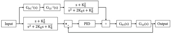
Figure 18.
Layout of the control flow for the 2 DOF controller. The values of , , and were taken from the tuned PID controllers for each activation level.
Table 11.
Tuned 2 DOF controller coefficients.
Once the controllers were designed, they were implemented on an ESP32 microcontroller and tested to determine their performance in controlling the actuator. To do so, actuating modules were constructed in a horizontal configuration, as in the force characterisation experiment, except with three pairs of TCAs instead of six. Once the actuator was woven, the load cell structure was adjusted to ensure that a 45° pennation angle was maintained, after which, each control scheme was tested. During the experiment run time, a pair of TCAs were chosen randomly and heated via PWM (100 ms cycle time) with a maximum supplied power of 80 W per active pair of TCAs at 20 V and 4 A. This was done until it reached a specified force setpoint based on the number of active pairs, which were determined based on the results of the force characterisation experiment. The force output of the actuator was maintained until five seconds had elapsed after achieving the desired setpoint value. The actuator was then allowed to cool until the force readings again reached zero, when another random pair of TCAs would be selected and the process would begin again. Five trials were performed in this way using the PID controller, then five using the 2 DOF controller. The number of active TCAs was then increased by one, the power supplied to the actuator was increased by 80 W, and the force setpoint was increased to match the new number of active TCAs. This was repeated until each controller had been tested five times at each activation level on that actuator. This entire process was then repeated on further actuators until three actuators had been tested, giving 15 trials per activated pair for each type of controller.
3.2. Results
After completing the force control experiments, the data collected were processed and made usable for analysis. The first segment of data consisting of the time it took to reach the force setpoint, plus an additional five seconds, was separated from the rest of the data, as that was the controlled portion of each trial. These data can be seen in Figure 19 for the PID-controlled and the 2 DOF-controlled experiments. After separating the data in this manner, the time constant, rise time, first peak time, overshoot, and settling value were calculated from the force responses. Using these calculated values, confidence intervals were constructed for each of the activation levels for each of the two types of controller tested, and the average steady state errors were also calculated. These can be seen in Figure 20.
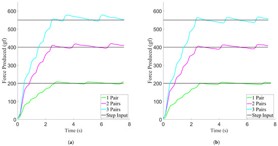
Figure 19.
Force responses of the force control implementation experiments, showing data from example trials. For the purpose of clarity, example curves were used due to low variance between trials. (a) PID controller force response. (b) 2 DOF controller force response.
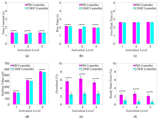
Figure 20.
Calculated control performance values for the PID and 2 DOF controller implementation experiments, compared to activation level. A ∗ denotes a grouping with a significant difference. All p values < 0.01. (a) Time constant values. (b) Rise time values. (c) First peak time values. (d) Settling values. (e) Percent overshoot values. (f) Percent steady state error values.
Comparing between the PID and 2 DOF controller, it was found that there were statistically significant differences in regards to the time constant, rise time, overshoot, and settling value ( comparing within the same activation level), while the first peak times were not statistically significantly different () within the same activation level. This indicates that the amount of error between the two controllers was statistically different, from the overshoot and settling value results, while having similar response times due to the lack of difference between the first peak times. It also indicates that the two controllers have different transient behaviours, from the results of the time constant and rise time comparisons.
3.3. Discussion
Looking at the constructed confidence intervals of the control performance values (seen in Figure 20), it is clear that the 2 DOF controller was the least erroneous of the two, having between 2.4% and 2.6% overshoot, and between 0.56% and 0.94% steady state error, while the PID controller had between 5.3% and 6.2% overshoot, and between 2.02% and 2.31% steady state error. The 2 DOF controller was able to minimize the error present in the system, while having minimal impact on response time, being statistically similar to the PID controller. As well, the settling values tended to be below the force setpoints at each activation level, which is desirable, as it errs on the side of user safety in wearable scenarios. This is important when considering its intended incorporation into therapeutic devices. Therefore, of the two controllers, it can be said that with its conservative nature and greater accuracy, without sacrificing response time, the 2 DOF controller is the superior of the two.
4. Conclusions
The work presented in this paper aimed to develop a viable bi-pennate TCA-based actuation system, embedded in a woven mesh for use in wearable mechatronic rehabilitation devices. This was done by determining the isotonic stroke and isometric force production capabilities of the actuator, its contractive actuation period, its electrical-to-mechanical power conversion efficiency, and developing models to predict the transient stroke and force response of the system. From these created models, force control schemes were designed and tested to determine to what degree the actuator could be controlled, and which of the control schemes was best suited for the actuator’s intended purpose.
The results of the experiments found that the stroke and force production of the actuators scaled linearly with the number of activated TCAs, achieving a maximum force of 11.28 N, a maximum stroke of 12.23%, and a maximum efficiency of 1.8%, similar to results found in the literature. This efficiency was found to increase with actuation speed, meaning that there could be improvements with the use of more power. The linearity of its production indicates that the actuation module can be scaled to meet different stroke and force requirements. Different instances of the actuator had little variance between them, indicating repeatable, reliable actuation with different modules.
After developing temperature–force relationships for each activation level of the actuator, PID and 2 DOF force controllers were developed and tuned to minimize the overshoot and steady state error of a step force response. These operated exclusively on force feedback, as the goal was to minimize the complexity and cost of the system, which would impose barriers to adoption. The 2 DOF controller was found to be the more conservative of the two, with a maximum overshoot of 2.6% and a maximum steady state error of 0.94%. This was compared to the PID controller, which had a maximum overshoot of 6.2% and a maximum steady state error of 2.58%. This indicates that the 2 DOF controller would be preferred for therapeutic devices, as overshoot and steady state error represent possibilities of injuring the user. The 2 DOF controller was able to achieve a minimum contractive period of 2.60 s, only slightly higher than the uncontrolled minimum contraction period found of 2.43 s, but statistically insignificant from the baseline PID controller.
Despite these desirable results, there were some shortcomings with the designed actuation module. The efficiency was unable to be improved beyond other TCA implementations in the literature. As well, while the 2 DOF controller was able to minimize the error, it was unable to eliminate it completely, likely due to a combination of PWM ripple and the use of linear modelling and control methods to control a non-linear system. Finally, while the contraction speed could be improved through the addition of more power to the system, the cooling times of the system were very high, and prevent rapid cyclic motion, as would happen in regular therapeutic use. While many of these three limitations are non-ideal, all of them can and should be addressed in future work. To overcome the first, results indicated that increasing the power supply, in addition to increasing the contraction speed of the actuator, also increased its efficiency. More power should be applied to see to what degree this effect can increase its efficiency. More complex modes of modelling and control should be investigated to control the system and eliminate the error present in the system. Finally, a cooling system should be integrated with the design, to enable it to have relaxation speeds as fast as its contraction speeds. Future work should also look into other fabric materials, such as wool, which has shown to be a promising thermal regulating material suitable for actuating purposes [33], and other fabric making processes, such as knitting or crocheting, to see if the same performance can be obtained with alternative fabric meshes, which could also have different heating and cooling characteristics.
While the presence of these limitations indicates that further work is required to refine the design, the results show that the designed fabric actuator is a promising flexible actuator for use in wearable mechatronic devices, scaling to meet different requirements while being able to be accurately controlled in a timely manner with minimal additional components. This, in combination with the actuator’s flexibility, ease of manufacture, and low cost, make it an appealing possibility for inclusion in wearable devices. Although this work demonstrates the actuation module’s potential, further work is required to refine it before it can be incorporated in medical and commercial devices.
Author Contributions
Conceptualization, V.M.; data curation, V.M.; formal analysis, V.M.; methodology—save for TCA fabrication and training, V.M.; investigation, V.M.; software, V.M.; validation, V.M.; visualization, V.M.; writing—original draft, save for abstract; methodology—TCA fabrication and training, B.P.R.E.; writing—abstract, B.P.R.E.; troubleshooting assistance, B.P.R.E.; supervision, A.L.T.; project administration, A.L.T.; funding acquisition, A.L.T.; resources, A.L.T.; writing—review and editing, B.P.R.E. and A.L.T. All authors have read and agreed to the published version of the manuscript.
Funding
This research was funded by the following grants awarded to Dr. A.L. Trejos: the Natural Sciences and Engineering Research Council (NSERC) of Canada under grant RGPIN-2014-03815, the Canadian Foundation for Innovation (CFI), the Ontario Research Fund (ORF), and the Ontario Ministry of Economic Development, Trade and Employment and the Ontario Ministry of Research and Innovation through the Early Researcher Award.
Data Availability Statement
The data that support the findings of this study are available from the corresponding author, Ana Luisa Trejos, upon reasonable request.
Conflicts of Interest
The authors declare no conflict of interest. The funders had no role in the design of the study; in the collection, analyses, or interpretation of data; in the writing of the manuscript, or in the decision to publish the results.
Abbreviations
The following abbreviations are used in this manuscript:
| 2 DOF | 2-Degree of Freedom |
| ANOVA | Analysis of Variance |
| C. | Cooling |
| DC | Direct Current |
| H. | Heating |
| PID | Proportional-Integral-Derivative |
| PWM | Pulse Width Modulation |
| RMS | Root Mean Square |
| TCA | Twisted Coiled Actuator |
References
- Mackay, J.; Mensah, G. The Atlas of Heart Disease and Stroke; World Health Organization: Geneva, Switzerland, 2004; pp. 1–16. [Google Scholar]
- Krakauer, J.W. Arm function after stroke: From physiology to recovery. Semin. Neurol. 2005, 25, 384–395. [Google Scholar] [CrossRef] [PubMed]
- Tsagarakis, N.G.; Caldwell, D.G. Development and control of a ’soft-actuated’ exoskeleton for use in physiotherapy and training. Auton. Robot. 2003, 15, 21–33. [Google Scholar] [CrossRef]
- Elsner, B.; Kugler, J.; Pohl, M.; Mehrholz, J. Electromechanical and robot-assisted arm training for improving activities of daily living, arm function, and arm muscle strength after stroke (review). Cochrane Libr. Database Syst. Rev. 2018, 2018, 1–136. [Google Scholar]
- Sulzer, J.S.; Peshkin, M.A.; Patton, J.L. Design of a mobile, inexpensive device for upper extremity rehabilitation at home. In Proceedings of the 2007 IEEE 10th International Conference on Rehabilitation Robotics, Noordwijk, The Netherlands, 12–15 June 2007; pp. 933–937. [Google Scholar]
- Cherry, C.O.; Chumbler, N.R.; Richards, K.; Huff, A.; Wu, D.; Tilghman, L.M.; Butler, A. Expanding stroke telerehabilitation services to rural veterans: A qualitative study on patient experiences using the robotic stroke therapy delivery and monitoring system program. Disabil. Rehabil. Assist. Technol. 2017, 12, 21–27. [Google Scholar] [CrossRef] [PubMed]
- Tang, X.; Li, K.; Liu, Y.; Zhou, D.; Zhao, J. A general soft robot module driven by twisted and coiled actuators. Smart Mater. Struct. 2019, 28, 1–14. [Google Scholar] [CrossRef]
- Haines, C.S.; Lima, M.D.; Li, N.; Spinks, G.M.; Foroughi, J.; Madden, J.D.W.; Kim, S.H.; Fang, S.; de Andrade, M.J.; Goktepe, F.; et al. Artificial muscles from fishing line and sewing thread. Science 2014, 343, 868–872. [Google Scholar] [CrossRef] [PubMed]
- Mirvakili, S.M.; Rafie Ravandi, A.; Hunter, I.W.; Haines, C.S.; Li, N.; Foroughi, J.; Naficy, S.; Spinks, G.M.; Baughman, R.H.; Madden, J.D.W. Simple and strong: Twisted silver painted nylon artificial muscle actuated by Joule heating. In Proceedings of the SPIE Smart Structures and Materials and Nondestructive Evaluation and Health Monitoring, San Diego, CA, USA, 9–13 March 2014; pp. 1–10. [Google Scholar]
- Yip, M.C.; Niemeyer, G. On the control and properties of supercoiled polymer artificial muscles. IEEE Trans. Robot. 2017, 33, 689–699. [Google Scholar] [CrossRef]
- Edmonds, B.P.R.; DeGroot, C.; Trejos, A.L. Thermal Modeling and Characterization of Twisted Coiled Actuators for Upper Limb Wearable Devices. IEEE/ASME Trans. Mechatron. 2020. [Google Scholar] [CrossRef]
- Maziz, A.; Concas, A.; Khaldi, A.; Stålhand, J.; Persson, N.K.; Jager, E.W. Knitting and weaving artificial muscles. Sci. Adv. 2017, 3, 1–11. [Google Scholar] [CrossRef] [PubMed]
- Kianzad, S.; Pandit, M.; Lewis, J.D.; Berlingeri, A.R.; Haebler, K.J.; Madden, J.D.W. Variable stiffness and recruitment using nylon actuators arranged in a pennate muscle configuration. In Proceedings of the Electroactive Polymer Actuators and Devices (EAPAD) 2015, San Diego, CA, USA, 9–12 March 2015; pp. 1–5. [Google Scholar]
- Liu, S.; Tang, X.; Zhou, D.; Liu, Y. Fascicular module of nylon twisted actuators with large force and variable stiffness. Sens. Actuators Phys. 2020, 315, 1–11. [Google Scholar] [CrossRef]
- Azizi, E.; Roberts, T.J. Variable gearing in a biologically inspired pneumatic actuator array. Bioinspir. Biomim. 2013, 8, 1–8. [Google Scholar] [CrossRef] [PubMed]
- Polygerinos, P.; Wang, Z.; Galloway, K.C.; Wood, R.J.; Walsh, C.J. Soft robotic glove for combined assistance and at-home rehabilitation. Robot. Auton. Syst. 2015, 73, 135–143. [Google Scholar] [CrossRef]
- Cho, K.H.; Song, M.G.; Jung, H.; Yang, S.Y.; Moon, H.; Koo, J.C.; Nam, J.D.; Choi, H.R. Fabrication and modeling of temperature-controllable artificial muscle actuator. In Proceedings of the IEEE International Conference on Biomedical Robotics and Biomechatronics, UTown, Singapore, 26–29 June 2016; pp. 94–98. [Google Scholar]
- Abbas, A.; Zhao, J.; Bradley, T.; Maciejewski, A. Modelling of Twisted and Coiled Artificial Muscle for Actuation and Self-Sensing. Ph.D. Thesis, Colorado State University, Fort Collins, CO, USA, 2018; pp. 1–60. [Google Scholar]
- Tadesse, Y.; Wu, L.; Karami, F.; Hamidi, A. Biorobotic systems design and development using TCP muscles. In Proceedings of the Electroactive Polymer Actuators and Devices (EAPAD) 2018, Denver, CO, USA, 5–8 March 2018; pp. 1–11. [Google Scholar]
- Kianzad, S.; Pandit, M.; Bahi, A.; Rafie Ravandi, A.; Ko, F.; Spinks, G.M.; Madden, J.D.W. Nylon coil actuator operating temperature range and stiffness. In Proceedings of the SPIE Smart Structures and Materials + Nondestructive Evaluation and Health Monitoring, San Diego, CA, USA, 8–12 March 2015; pp. 1–6. [Google Scholar]
- Buckner, T.L.; Kramer-Bottiglio, R. Functional fibers for robotic fabrics. Multifunct. Mater. 2018, 1, 1–22. [Google Scholar] [CrossRef]
- Hiramitsu, T.; Suzumori, K.; Nabae, H.; Endo, G. Experimental evaluation of textile mechanisms made of artificial muscles. In Proceedings of the IEEE International Conference on Soft Robotics (RoboSoft), Seoul, Korea, 14–18 April 2019; pp. 1–6. [Google Scholar]
- Xiang, C.; Sun, Z.; Hao, L.; Song, B. The design, hysteresis modeling and control of a novel SMA-fishing-line actuator. Smart Mater. Struct. 2017, 26, 1–11. [Google Scholar] [CrossRef]
- Yuen, M.; Cherian, A.; Case, J.C.; Seipel, J.; Kramer, R.K. Conformable actuation and sensing with robotic fabric. In Proceedings of the IEEE International Conference on Intelligent Robots and Systems, Chicago, IL, USA, 14–18 September 2014; pp. 580–586. [Google Scholar]
- Simeonov, A.; Henderson, T.; Lan, Z.; Sundar, G.; Factor, A.; Zhang, J.; Yip, M. Bundled super-coiled polymer artificial muscles: Design, characterization, and modeling. IEEE Robot. Autom. Lett. 2018, 3, 1671–1678. [Google Scholar] [CrossRef]
- Persson, N.K.; Martinez, J.G.; Zhong, Y.; Maziz, A.; Jager, E.W. Actuating textiles: Next generation of smart textiles. Adv. Mater. Technol. 2018, 3, 1–12. [Google Scholar] [CrossRef]
- Hiraoka, M.; Nakamura, K.; Arase, H.; Asai, K.; Kaneko, Y.; John, S.W.; Tagashira, K.; Omote, A. Power-efficient low-temperature woven coiled fibre actuator for wearable applications. Sci. Rep. 2016, 6, 1–9. [Google Scholar] [CrossRef]
- Liu, Y.; Zang, X.; Lin, Z.; Li, W.; Zhao, J. Position control of a bio-inspired semi-active joint with direct inverse hysteresis modeling and compensation. Adv. Mech. Eng. 2016, 8, 1–8. [Google Scholar] [CrossRef]
- Arakawa, T.; Takagi, K.; Tahara, K.; Asaka, K. Position control of fishing line artificial muscles (coiled polymer actuators) from nylon thread. In Proceedings of the Electroactive Polymer Actuators and Devices (EAPAD) 2016, Las Vegas, NV, USA, 21–24 March 2016; pp. 1–12. [Google Scholar]
- Suzuki, M.; Kamamichi, N. Displacement control of an antagonistic-type twisted and coiled polymer actuator. Smart Mater. Struct. 2018, 27, 1–11. [Google Scholar] [CrossRef]
- Incropera, F. Fundamentals of Heat and Mass Transfer, Vol. 6; Wiley: Hoboken, NJ, USA, 2006; pp. 288–289. [Google Scholar]
- Edmonds, B.P.; Trejos, A.L. Computational fluid dynamics study of a soft actuator for use in wearable mechatronic devices. In Proceedings of the IEEE RAS and EMBS International Conference on Biomedical Robotics and Biomechatronics, Enschede, The Netherlands, 26–29 August 2018; pp. 1333–1338. [Google Scholar]
- Hu, J.; Irfan Iqbal, M.; Sun, F. Wool Can Be Cool: Water-Actuating Woolen Knitwear for Both Hot and Cold. Adv. Funct. Mater. 2020, 30, 1–9. [Google Scholar] [CrossRef]
Publisher’s Note: MDPI stays neutral with regard to jurisdictional claims in published maps and institutional affiliations. |
© 2021 by the authors. Licensee MDPI, Basel, Switzerland. This article is an open access article distributed under the terms and conditions of the Creative Commons Attribution (CC BY) license (http://creativecommons.org/licenses/by/4.0/).