
Optimization of the Guiding Stability of a Horizontal Axis HTS ZFC Radial Levitation Bearing

 ,
,  ,
,  and
and 
Abstract
:1. Introduction
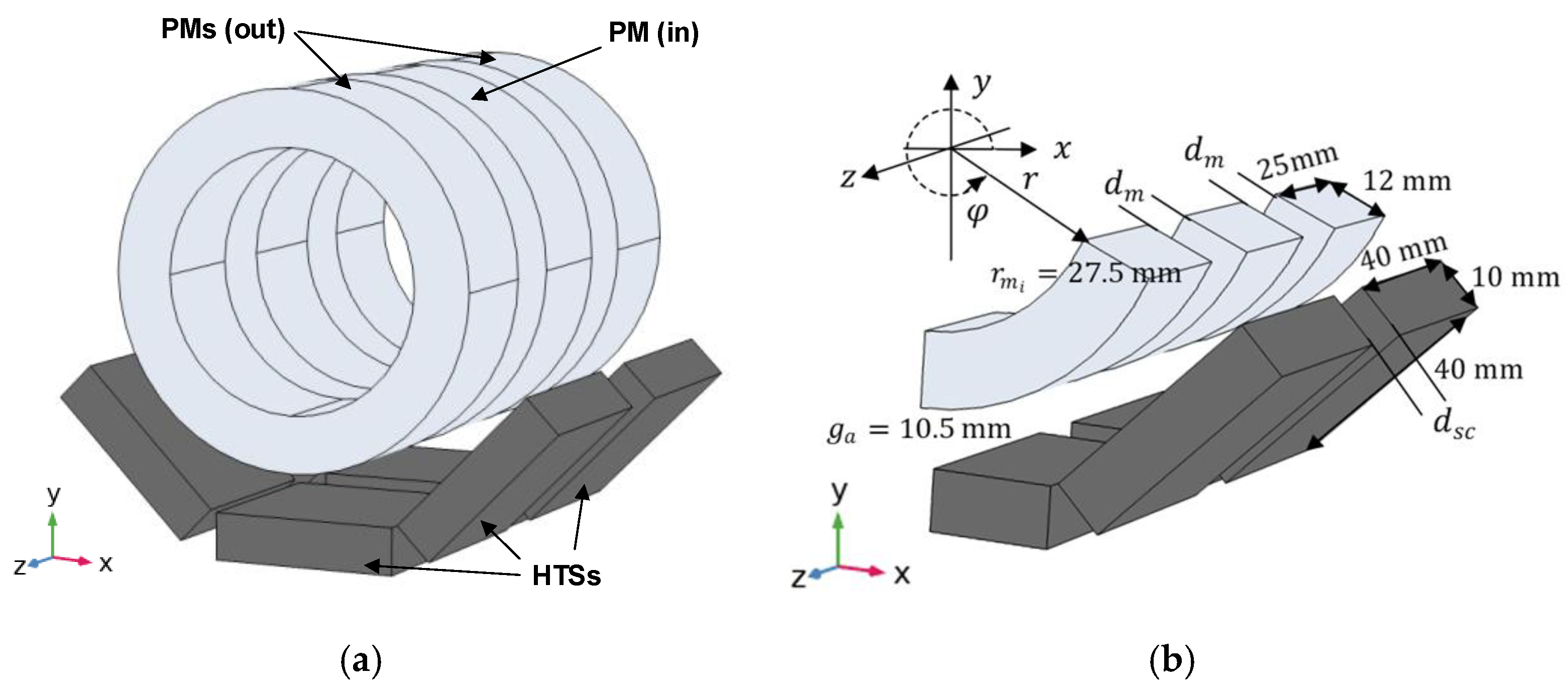
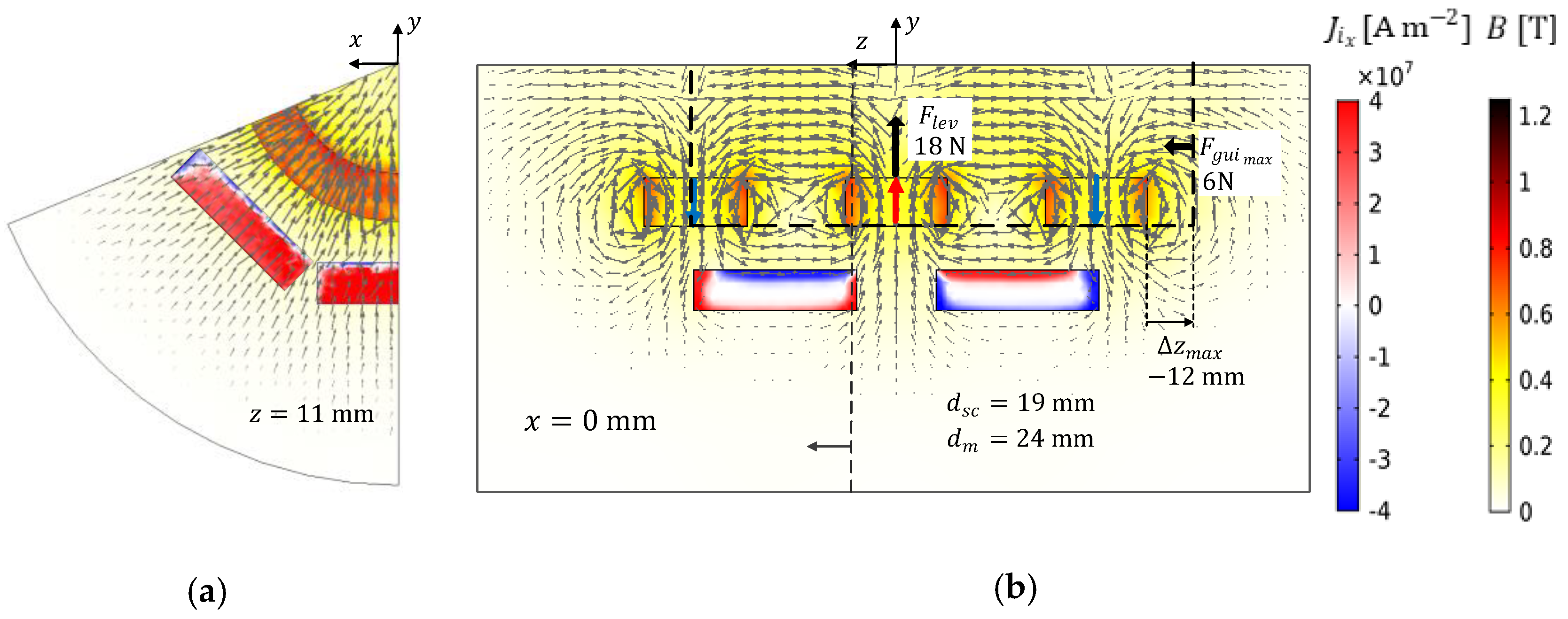
2. Electromagnetic Models and Parameters
2.1. E-J Model
2.2. Equivalent Relative Permeability Model
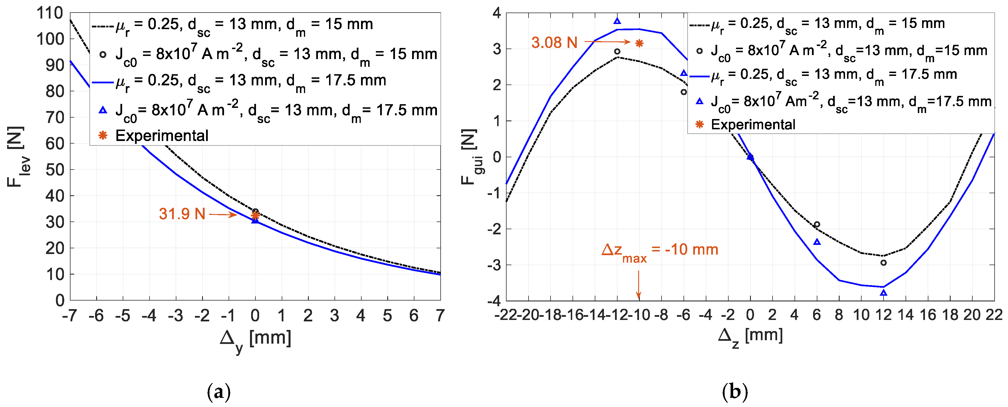
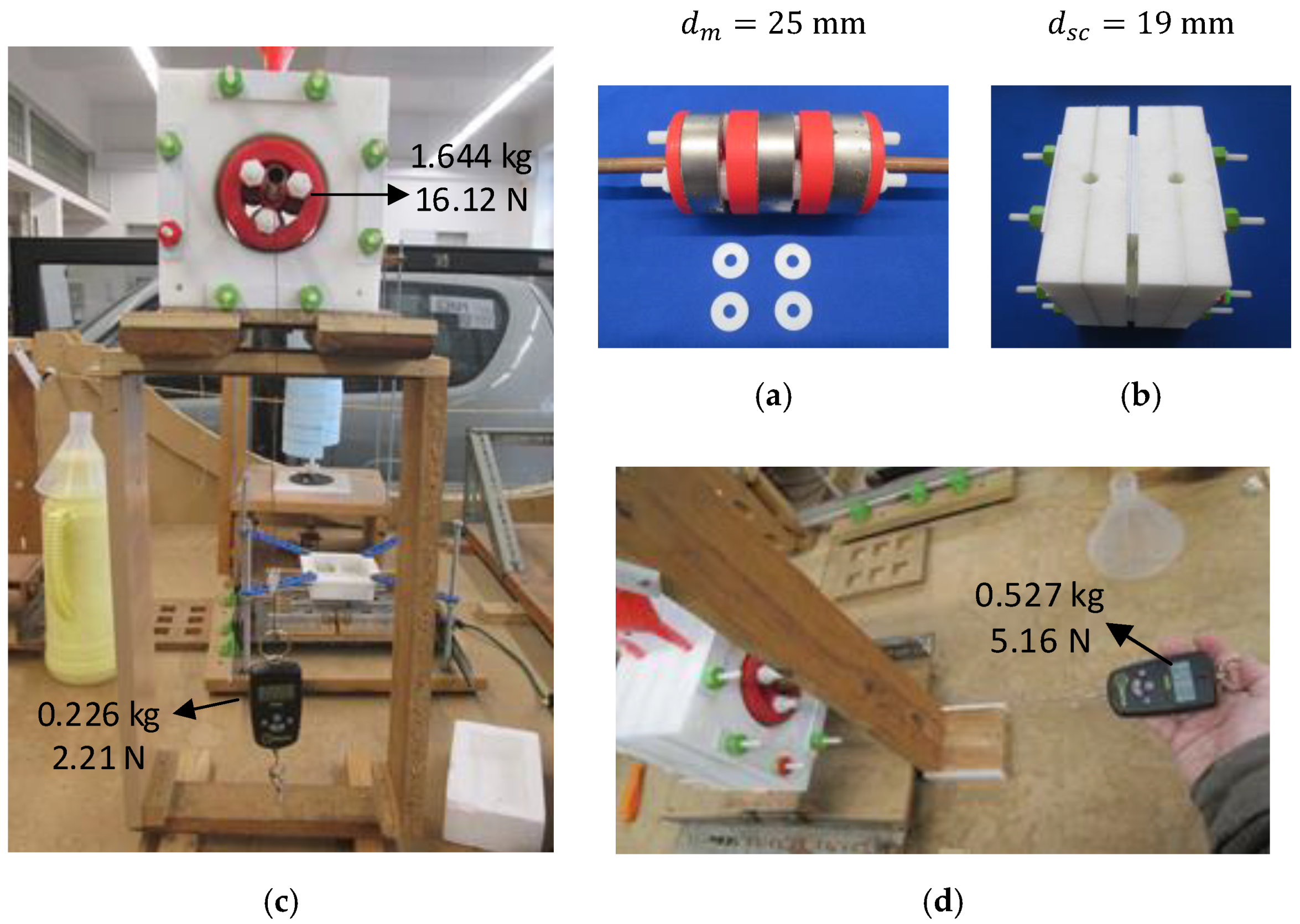
3. Validation of Electromagnetic Model Parameters
4. Characterization of Dynamics for the Configuration with Six Bulks at the Bottom of Stator I
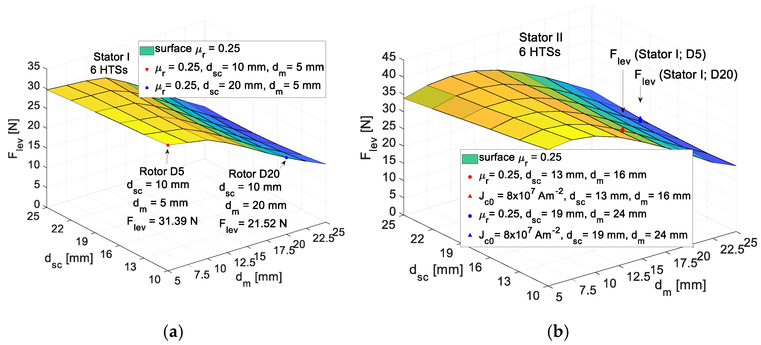
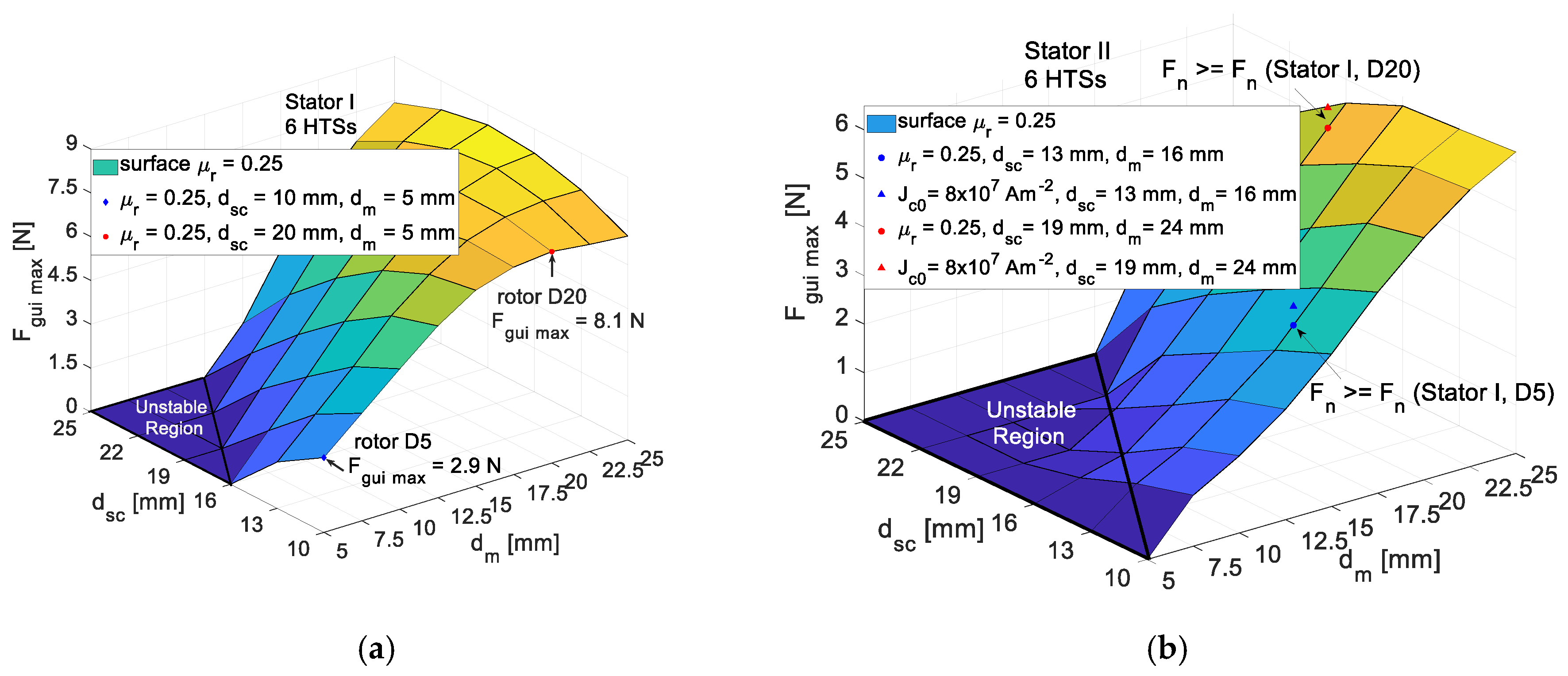
5. Optimization of the HTS and PM Ring Spacing to Maximize the Guiding Stability
5.1. Optimization Methodology
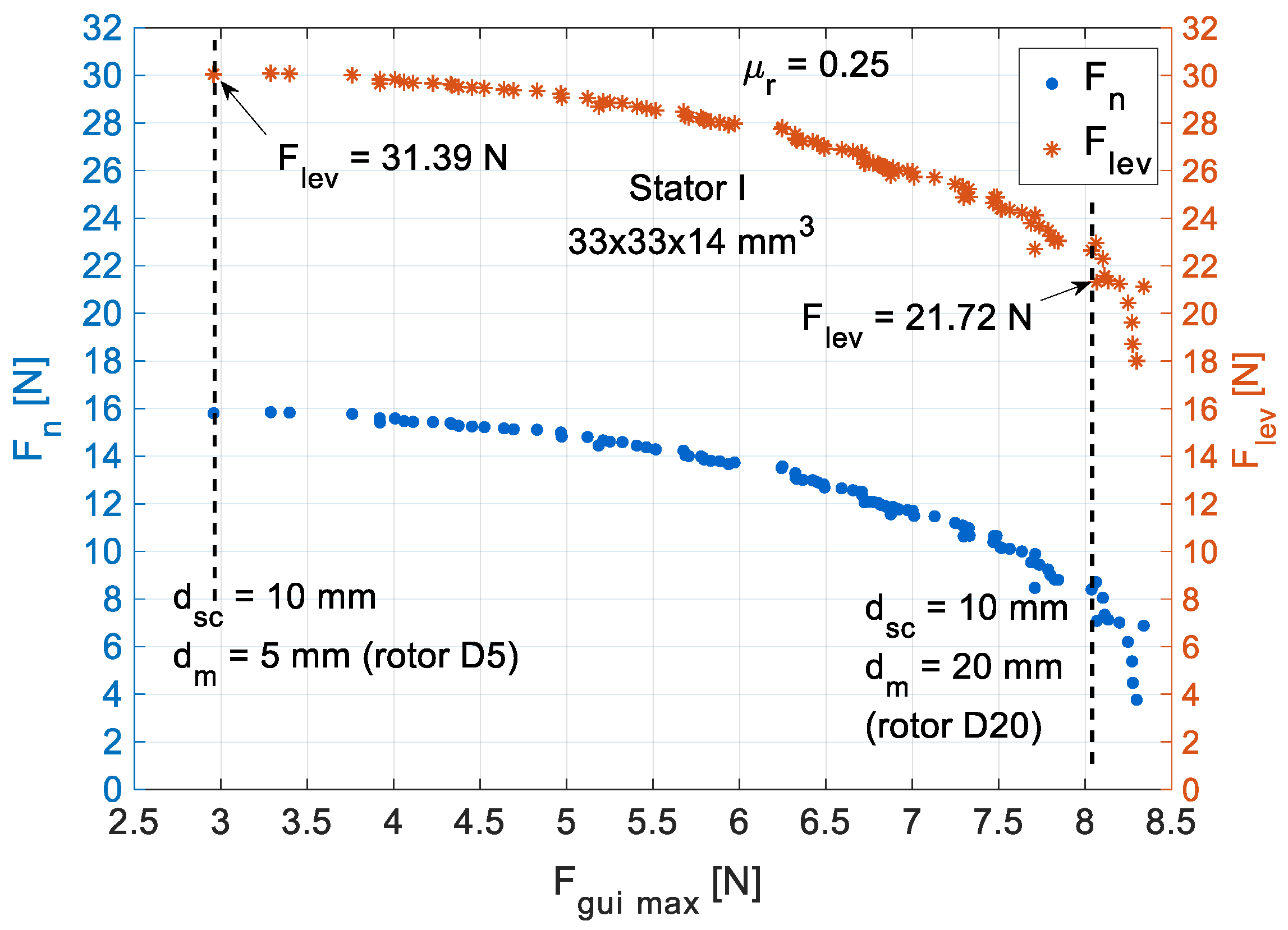
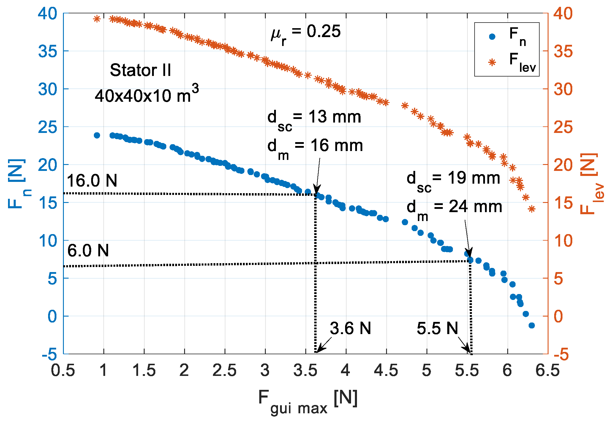
5.2. Optimization Results
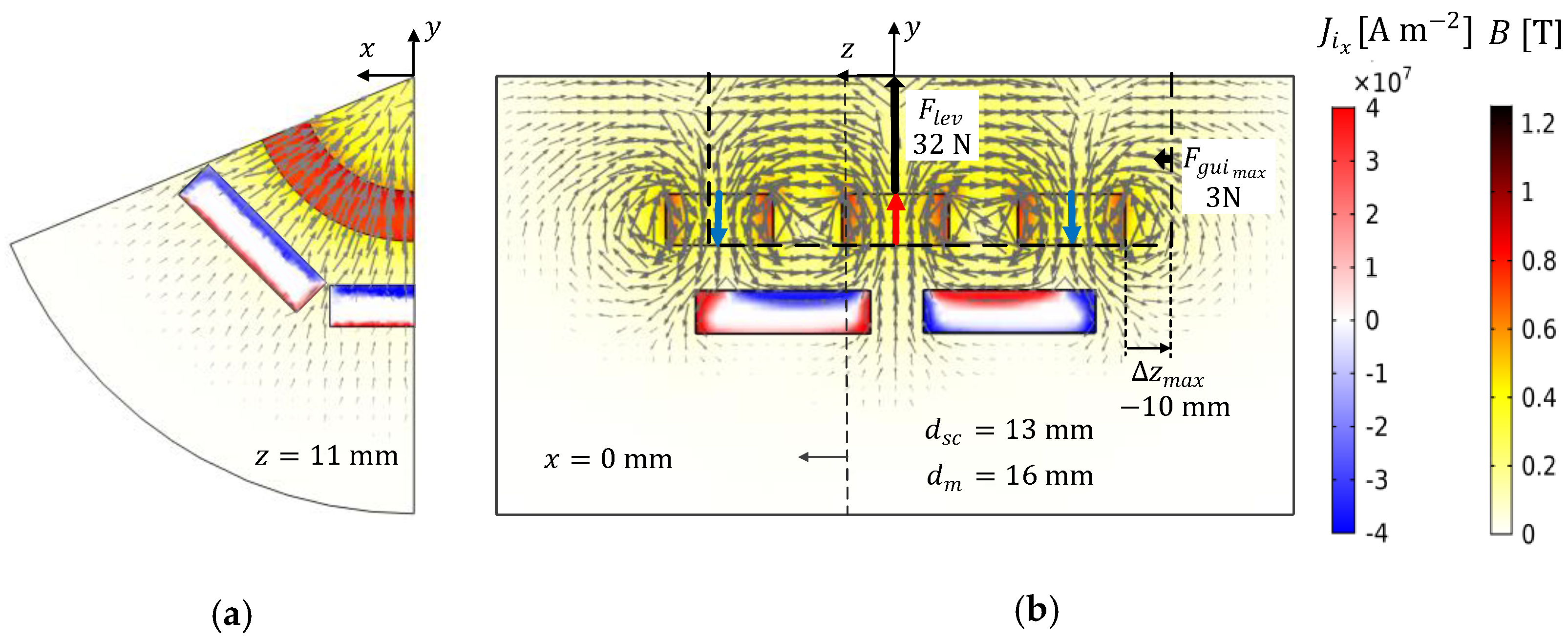
6. Identification of Guiding Stability Zones
7. Conclusions
Author Contributions
Funding
Acknowledgments
Conflicts of Interest
References
- Arsénio, A.J.; Carvalho, M.V.; Cardeira, C.; Branco, P.J.C.; Melício, R. Conception of a YBCO superconducting ZFC-magnetic bearing virtual prototype. In Proceedings of the IEEE International Power Electronics and Motion Control Conference (PEMC), Varna, Bulgaria, 25–28 September 2016. [Google Scholar]
- Arsenio, A.J.; Roque, M.; Cardeira, C.; Branco, P.J.C.; Melicio, R. Prototype of a Zero-Field-Cooled YBCO Bearing with Continuous Ring Permanent Magnets. IEEE Trans. Appl. Supercond. 2018, 28, 1–7. [Google Scholar] [CrossRef]
- Arsenio, A.J.; Melicio, R.; Cardeira, C.; Branco, P.J.D.C. The Critic Liquid–Gas Phase Transition between Liquid Nitrogen and YBCO HTS Bulks: From FEM Modeling to its Experimental Study for ZFC Levitation Devices. IEEE Trans. Appl. Supercond. 2018, 28, 1–8. [Google Scholar] [CrossRef]
- Arsenio, A.J.C.; Branco, P.J.C. Thermo-Hydraulic Analysis of a Horizontal HTS ZFC Levitating Bearing Concerning Its Autonomy Safety Service Time. IEEE Trans. Appl. Supercond. 2021, 31, 1–10. [Google Scholar] [CrossRef]
- Queval, L.; Sotelo, G.; Kharmiz, Y.; Dias, D.H.N.; Sass, F.; Zermeno, V.M.R.; Gottkehaskamp, R. Optimization of the Superconducting Linear Magnetic Bearing of a Maglev Vehicle. IEEE Trans. Appl. Supercond. 2016, 26, 1–5. [Google Scholar] [CrossRef] [Green Version]
- Fernandes, J.F.P.; Costa, A.J.A.; Arnaud, J.; Arsenio, A.J. Optimization of a Horizontal Axis HTS ZFC Levitation Bearing Using Genetic Decision Algorithms over Finite Element Results. IEEE Trans. Appl. Supercond. 2020, 30, 1–8. [Google Scholar] [CrossRef]
- Schultz, L.; De Haas, O.; Verges, P.; Beyer, C.; Rohlig, S.; Olsen, H.; Kuhn, L.; Berger, D.; Noteboom, U.; Funk, U. Superconductively Levitated Transport System—The SupraTrans Project. IEEE Trans. Appl. Supercond. 2005, 15, 2301–2305. [Google Scholar] [CrossRef]
- Sotelo, G.G.; Dias, D.H.N.; de Andrade, R., Jr.; Stephan, R.M. Tests on a Superconductor Linear Magnetic Bearing of a Full-Scale Maglev Vehicle. IEEE Trans. Appl. Supercond. 2011, 21, 1464–1468. [Google Scholar] [CrossRef]
- Yang, W.; Wen, Z.; Duan, Y.; Chen, X.; Qiu, M.; Liu, Y.; Lin, L. Construction and Performance of HTS Maglev Launch Assist Test Vehicle. IEEE Trans. Appl. Supercond. 2006, 16, 1108–1111. [Google Scholar] [CrossRef]
- di Barba, P.; Palka, R. Optimization of the HTSC-PM Interaction in Magnetic Bearings by a Multiobjective Design, Intelligent Computer Techniques in Applied Electromagnetics; Studies in Computational Intelligence; Springer: Berlin/Heidelberg, Germany, 2008; pp. 54–59. [Google Scholar]
- Di Barba, P.; May, H.; Mognaschi, M.; Palka, R.; Savini, A. Multiobjective design optimization of an excitation arrangement used in superconducting magnetic bearings. Int. J. Appl. Electromagn. Mech. 2009, 30, 127–134. [Google Scholar] [CrossRef]
- Mateev, V.; Todorova, M.; Marinova, I. Eddy Current Losses of Coaxial Magnetic Gears. In Proceedings of the 2018 XIII International Conference on Electrical Machines (ICEM), Alexandroupoli, Greece, 3–6 September 2018; pp. 1157–1162. [Google Scholar]
- Usman, H.; Ikram, J.; Alimgeer, K.; Yousuf, M.; Bukhari, S.; Ro, J.-S. Analysis and Optimization of Axial Flux Permanent Magnet Machine for Cogging Torque Reduction. Mathematics 2021, 9, 1738. [Google Scholar] [CrossRef]
- Nguyen, H.P.; Nguyen, X.B.; Bui, T.T.; Ueno, S.; Nguyen, Q.D. Analysis and Control of Slotless Self-Bearing Motor. Actuators 2019, 8, 57. [Google Scholar] [CrossRef] [Green Version]
- Toh, C.S.; Chen, S.-L. Design, Modeling and Control of Magnetic Bearings for a Ring-Type Flywheel Energy Storage System. Energies 2016, 9, 1051. [Google Scholar] [CrossRef] [Green Version]
- Hong, Z.; Campbell, H.M.; Coombs, T.A. Computer Modeling of Magnetisation in High Temperature Superconductors. IEEE Trans. Appl. Supercond. 2007, 17, 3761–3764. [Google Scholar] [CrossRef]
- Yamamoto, K.; Mazaki, H.; Yasuoka, H. Magnetization of type-II superconductors in the Kim-Anderson model. Phys. Rev. B 1993, 47, 915–924. [Google Scholar] [CrossRef] [PubMed]
- Fujishiro, H.; Naito, T. Simulation of temperature and magnetic field distribution in superconducting bulk during pulsed field magnetization. Supercond. Sci. Technol. 2010, 23, 105021. [Google Scholar] [CrossRef] [Green Version]
- Koo, J.H.; Cho, G. Magnetic field dependence on transition temperature Tc in cuprate superconductors. Solid State Commun. 2004, 129, 191–193. [Google Scholar] [CrossRef]
- Zhang, M.; Coombs, T.A. 3D modeling of high-Tc superconductors by finite element software. Supercond. Sci. Technol. 2012, 25, 015009. [Google Scholar] [CrossRef]
- Peixoto, I.S.P.; da Silva, F.F.; Fernandes, J.F.P.; Branco, P.J.D.C. 3D Equivalent Space-Varying Permeability Model of HTS Bulks for Computation of Electromagnetic Forces. IEEE Trans. Appl. Supercond. 2021, 31, 1–7. [Google Scholar] [CrossRef]
- Fernandes, J.F.P. Comparison of fast computing methods for ZFC High-temperature superconductors bulks. Supercond. Sci. Technol. 2020, 33, 085001. [Google Scholar] [CrossRef]
- COMSOL Multiphysics 3. Available online: http://www.comsol.com (accessed on 11 January 2012).


| Stator | Number of HTS rings & LN2 chambers | Two |
| Maximum number bulks per chamber | Eight uniformly distributed | |
| Number of bulks in tested topologies | Three at the bottom of each chamber | |
| Height and width of the exterior surface | ||
| Total length with two LN2 chambers | 100 mm for Stator I 108 mm for Stator II | |
| Volume of each LN2 chamber | ||
| Diameter of the rotor cavity | ||
| Material of chamber walls | Rigid polyurethane of 40 kg m−3 | |
| Composite of HTS bulks | YBa2C3O7 crystal by TSMG | |
| Size of HTS bulks | in Stator I in Stator II | |
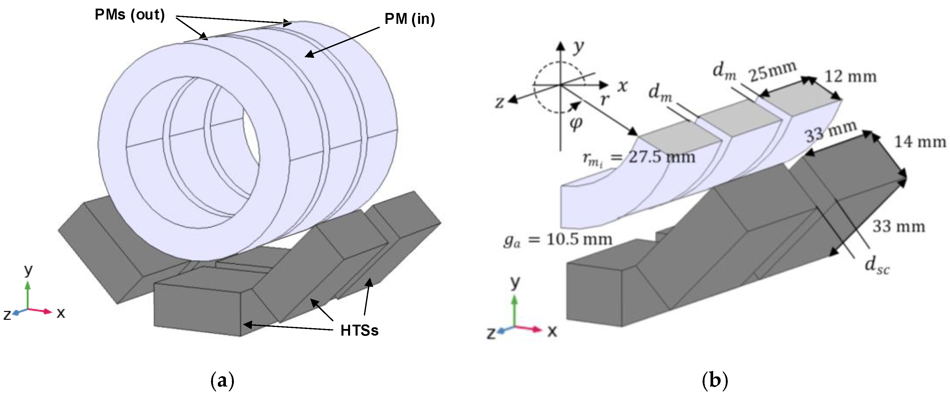
| Rotor | Number of PM rings | Three |
| Direction of magnetization | Radial | |
| Arrangement of polarizations | Alternate parallel | |
| Outer diameter of rotor and PM rings | ||
| Inner diameter of PM rings | ||
| Material of rotor structure | 3D printed PLA | |
| Composite of PMs | NdFeB of grade N40 () | |
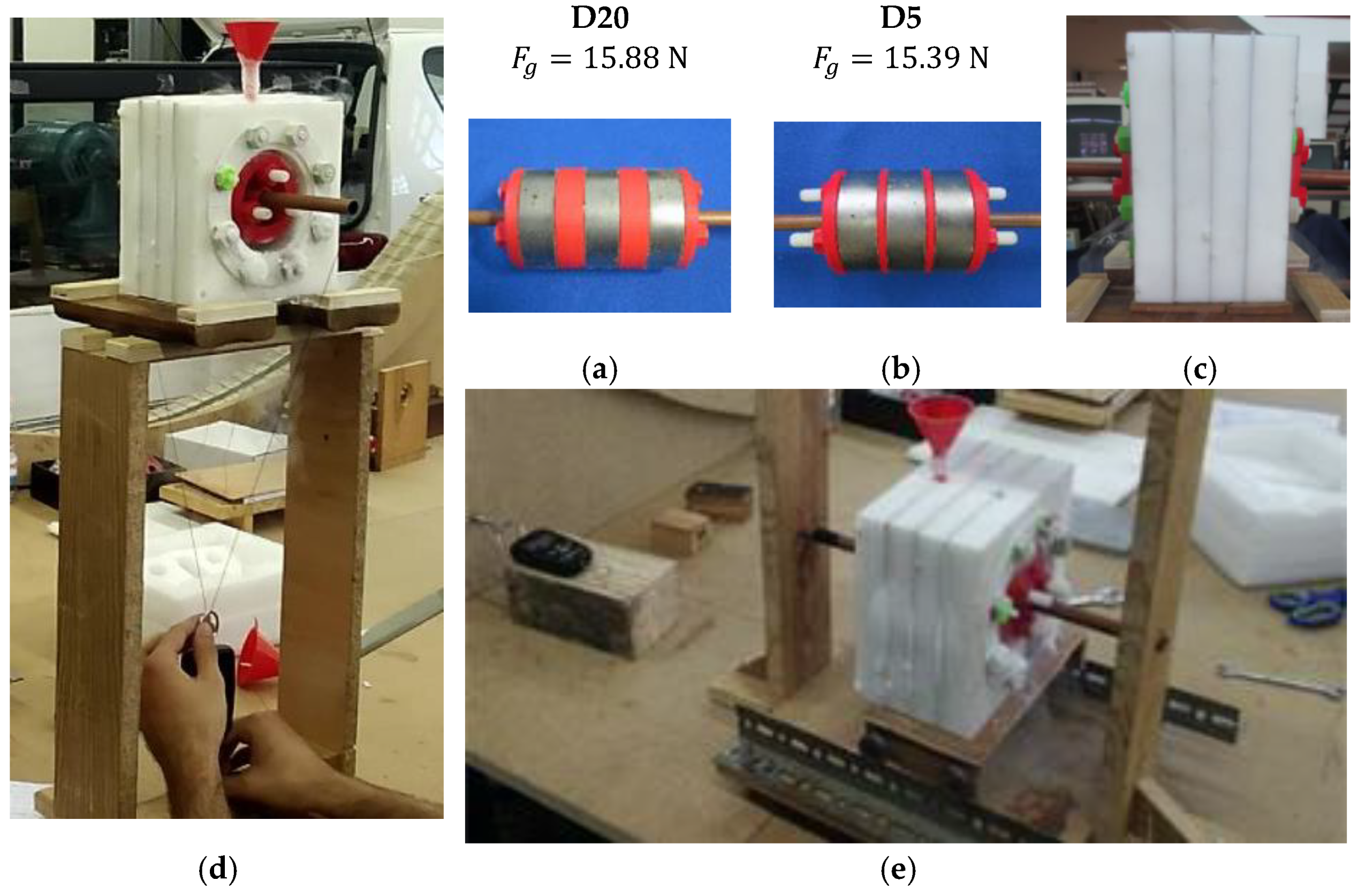
| Length of rotors | for Rotor D5 for Rotor D20 | |
| Weight and Gravity force | 1.57 kg & 15.39 N for Rotor D5 1.62 kg & 15.88 N for Rotor D20 | |
| Momentum of inertia | for Rotor D5 for Rotor D20 |
| Predicted Forces and Error ] from Measured Forces | Fn [N] Exp. | |||||||
|---|---|---|---|---|---|---|---|---|
0.2 | 0.25 | 0.3 | 0.4 | 3 × 10⁷ Am−2 | 8 × 10⁷ Am−2 | Exp. | ||
| Rotor D20 Fg = 15.88 N | 25.15 +31% | 22.72 +18.4% | 20.47 +6.67% | 16.40 −14.5% | 18.47 −3.75% | 23.73 +23.7% | 19.19 | 3.31 |
| Rotor D5 | 37.62 +24.3% | 31.39 +3.73% | 26.17 −13.5% | 21.44 −29.1% | 22.42 −25.9% | 32.31 +6.8% | 30.26 | 14.87 |
| Decision Variable | Description | Range [mm] |
|---|---|---|
| Spacing between PM rings with Stator I | 5–40 | |
| Spacing between PM rings with Stator II | 5–50 | |
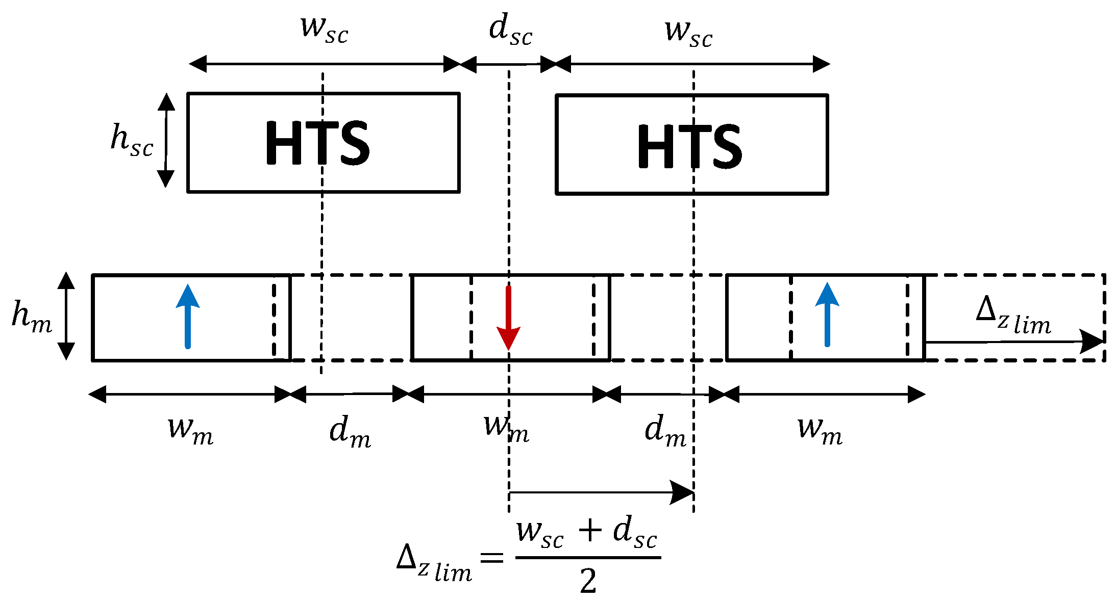
| Spacing between rings of HTS bulks | 10–30 |
| Minimum dm [mm] | ||
|---|---|---|
| dsc [mm] | Stator I | Stator II |
| 10 | 0.5 | 7.5 |
| 13 | 2 | 9 |
| 16 | 3.5 | 10.5 |
| 19 | 5 | 12 |
| 22 | 6.5 | 13.5 |
| 25 | 8 | 15 |
Publisher’s Note: MDPI stays neutral with regard to jurisdictional claims in published maps and institutional affiliations. |
© 2021 by the authors. Licensee MDPI, Basel, Switzerland. This article is an open access article distributed under the terms and conditions of the Creative Commons Attribution (CC BY) license (https://creativecommons.org/licenses/by/4.0/).
Share and Cite
Arsénio, A.J.; da Silva, F.F.; Fernandes, J.F.P.; Costa Branco, P.J. Optimization of the Guiding Stability of a Horizontal Axis HTS ZFC Radial Levitation Bearing. Actuators 2021, 10, 311. https://doi.org/10.3390/act10120311
Arsénio AJ, da Silva FF, Fernandes JFP, Costa Branco PJ. Optimization of the Guiding Stability of a Horizontal Axis HTS ZFC Radial Levitation Bearing. Actuators. 2021; 10(12):311. https://doi.org/10.3390/act10120311
Chicago/Turabian StyleArsénio, António J., Francisco Ferreira da Silva, João F. P. Fernandes, and Paulo J. Costa Branco. 2021. "Optimization of the Guiding Stability of a Horizontal Axis HTS ZFC Radial Levitation Bearing" Actuators 10, no. 12: 311. https://doi.org/10.3390/act10120311
APA StyleArsénio, A. J., da Silva, F. F., Fernandes, J. F. P., & Costa Branco, P. J. (2021). Optimization of the Guiding Stability of a Horizontal Axis HTS ZFC Radial Levitation Bearing. Actuators, 10(12), 311. https://doi.org/10.3390/act10120311