
Testing Bernard’s Thesis of His and Hers Marriage Using Marital Satisfaction Research Published Between 1929 and 1950



Abstract
1. Background
2. Literature Review
3. Research Problem, Questions, and Hypotheses
4. Methods

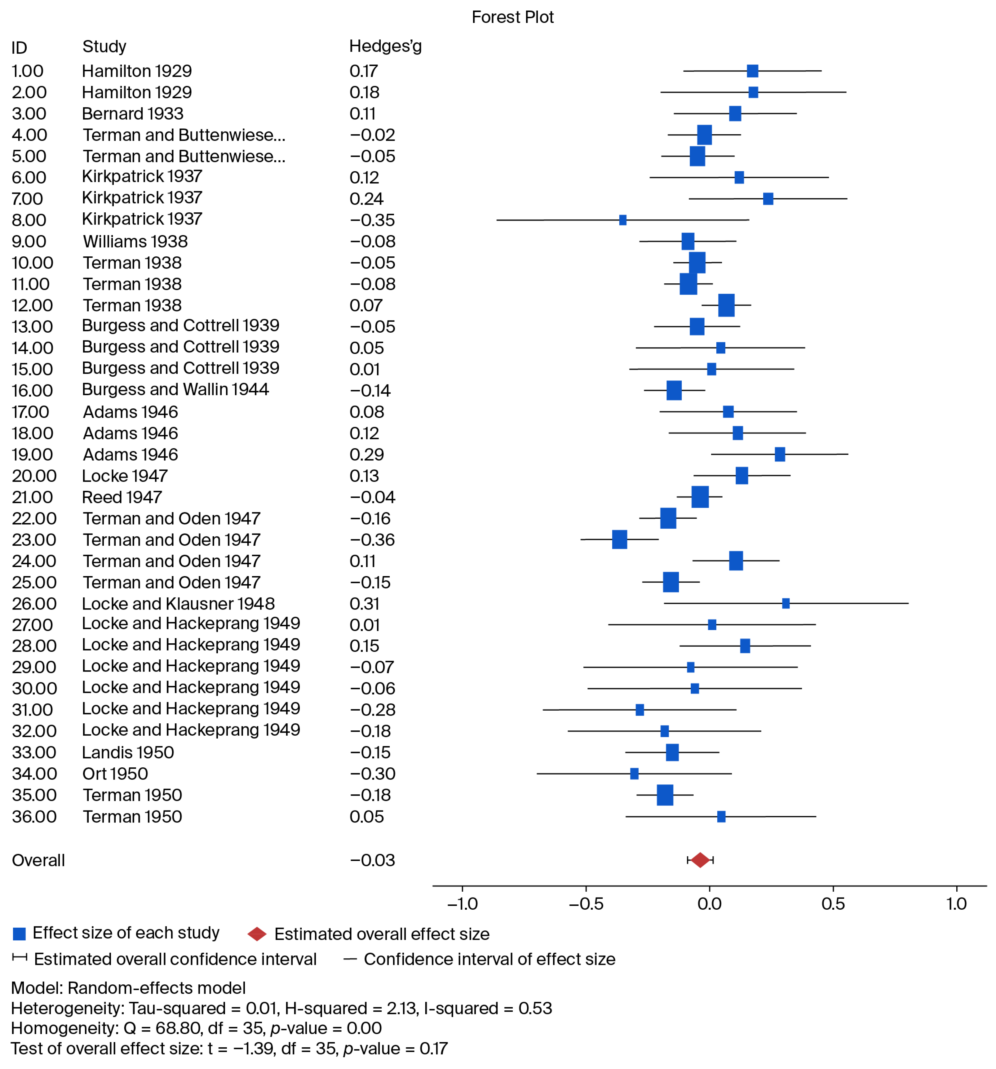
| Author | Date (Case Number) | Sample N | Mean (SD) Husbands | Mean (SD) Wives | t-Test Results + | Effect (Size) g/SE | Lower Satisfaction Ratio for Wives vs. Husbands |
|---|---|---|---|---|---|---|---|
| Hamilton (1929) | p. 79 (1) | 100 husbands | 6.58 | 5.92 | t(198) = 1.24 | 0.175 | 16:7 (scores of ≤1); data not provided |
| 100 wives | (3.70) | (3.82) | p = 0.216 | 0.1417 | |||
| p. 79 (2) | (15 wives/8 husbands divorced or separated) | 6.91 | 6.36 | t(108) = 0.96 | 0.179 | ||
| 55 heterosexual couples | [3.00] | [3.00] | p = 0.339, paired-sample data not provided | 0.1911 | |||
| Bernard (1933, 1934) | p. 197 (3) | 115 husbands 137 wives | 79.70 (17.0) | 77.90 (17.00) | t(250) = 0.403 p = 0.403 | 0.106 0.1266 | 6:4 (scores ≤ 38.50) |
| Terman and Buttenwieser (1935) | p. 162 (4) | 345 husbands | 46.20 | 46.44 | t(688) = −0.248 | −0.019 | 5:2 (scores of ≤5) |
| 345 wives | (12.46) | (12.71) | p = n.s. | 0.0761 | |||
| p. 167 (5) | 343 husbands | 4.17 | 4.21 | t(684) = −0.655 | −0.045 | 11:9 (scores of ≤2) | |
| 343 wives | (0.89) | (0.88) | p = n.s. | 0.0764 | |||
| Kirkpatrick (1937) | pp. 136–37 (6) | 58 husbands | 82.2 | 80.8 | t(114) = 0.66 | 0.122 | Data not provided |
| 58 wives | [12.75] | [9.95] | p = n.s. | 0.1859 | |||
| pp. 136–37 (7) | 70 husbands | 82.1 | 79.4 | t(150) = 1.47 | 0.237 | Data not provided | |
| 82 wives | [12.75] | [9.95] | p = 0.145 | 0.1633 | |||
| pp. 136–37 (8) | 30 husbands | 76.3 | 79.0 | t(58) = 1.13 | −0.348 | Data not provided | |
| 30 wives | [4.3] | [9.95] | p = 0.265 | 0.2603 | |||
| Williams (1938) | p. 48 (9) | 200 heterosexual couples | 151.25 (24.91) | 153.30 (23.38) | t(199) = 1.59 p = 0.114 r = 0.715 *** | −0.085 0.1000 | 8:4 cases (≥40 point difference) |
| Terman (1938) | p. 63 (10) | 792 husbands | 68.40 | 69.25 | t(1582) = −0.936 | −0.047 | 13:4 (scores < 10) 6:1 (extremely unhappy) |
| 792 wives | (17.35) | (18.75) | p = 0.349 | 0.0503 | |||
| p. 76 (11) | 792 husbands | 5.71 | 5.81 | t(1582) = −1.62 | −0.082 | ||
| 792 wives | (1.20) | (1.25) | p = 0.106 | 0.0503 | |||
| Terman (1938) | p. 78 (12) | 902 husbands 644 wives | 5.23 (1.62) | 5.11 (1.82) | t(1544) = 1.42 p = 0.154 | 0.070 0.0516 | 46:36 (scored lowest level of satisfaction, 1) |
| Burgess and Cottrell (1939) | p. 39 (13) | 251 couples | 4.20 (1.03) | 4.25 (1.03) | t(250) = −1.21 | −0.048 0.0893 | 6:3 (if difference is 2 points, wife less happy) |
| p = 0.226 | |||||||
| r = 0.815 *** | |||||||
| p. 70 (14) | 66 couples | 144.55 (38.01) | 142.73 (39.68) | t(65) = 0.78 | 0.047 0.1741 | 9:4 (if difference is 30 or more points, wife less happy) | |
| p = 0.439 | |||||||
| r = 0.882 *** | |||||||
| p. 285 (15) | 70 couples | 538.86 (99.32) | 537.71 (100.70) | t(69) = 0.199 | 0.011 0.1690 | 5:4 (difference of 80 points or more, wife less happy) | |
| p = 0.843 | |||||||
| r = 0.884 *** | |||||||
| Burgess and Wallin (1944) | p. 330 (16) | 505 heterosexual couples | 160.45 (20.04) | 163.14 (18.76) | t(1008) = −2.21 p = 0.028 | −0.138 0.0630 | 4:4 (scores < 100) |
| Adams (1946) | p. 187 (17) | 100 husbands | T: 76.85 | 75.95 | t(198) = 0.547 | 0.077 | Data not provided |
| (9.81) | (13.20) | p = 0.585 | 0.1415 | ||||
| p. 187 (18) | 100 wives | H: 10.55 | 10.22 | t(198) = 0.818 | 0.115 | Data not provided | |
| (2.70) | (3.00) | p = 0.415 | 0.1415 | ||||
| p. 187 (19) | 100 husbands; 100 wives | BC: 169.60 | 163.75 | t(198) = 2.03 | 0.285 | Data not provided | |
| (19.00) | (21.75) | p = 0.044 | 0.1422 | ||||
| Locke (1947) | p. 188 (20) | 200 couples | 167.3 (12.7, est.) | 165.6 (12.7, est.) | t(398) = 1.34 p = 0.182 | 0.134 0.1001 | 4.5%/2.5% of men/women had lowest scores |
| Reed (1947) | p. 387 (21) | 860 couples | 5.34 (1.36) | 5.39 (1.37) | t(1718) = −0.76 p = 0.448 | −0.037 0.0482 | 38:42 (scores ≤ 3) |
| Terman and Oden (1947) | p. 241 (22) | 556 husbands; 556 wives | 63.15 (19.76) | 66.34 (18.90) | t(1110) = −2.75 | −0.165 | 2:3 (scores ≤ 10) |
| p = 0.006 | 0.0601 | ||||||
| p. 244 (23) | 567 husbands; 567 wives | 5.93 (1.11) | 6.10 (1.10) | t(1132) = −2.69 | −0.154 | 12:7 (scores ≤ 2) | |
| p = 0.007 | 0.0595 | ||||||
| p. 245 (24) | 317 couples with gifted husbands | 59.50 (20.36) | 66.66 (19.30) | t(632) = −4.54 | −0.361 | Data not provided | |
| p < 0.0001 | 0.0801 | ||||||
| p. 245 (25) | 250 couples with gifted wives | 66.90 (18.80) | 64.86 (18.71) | t(498) = 1.22 | 0.109 | Data not provided | |
| p = 0.225 | 0.0895 | ||||||
| Locke and Klausner (1948) | p. 100 (26) | 31 husbands | 159 | 151 | t(62) = 1.26 | 0.311 | Data not provided |
| 33 wives | (25.4) | (25.4) | p = 0.213 | 0.2517 | |||
| Locke and Mackeprang (1949) | p. 536 (27) | 44 couples, wives employed | 168.2 | 167.8 | t(86) = 0.06 | 0.013 | Data not provided |
| (28.0) | (34.6) | p = n.s. | 0.2132 | ||||
| pp. 537–38 (28) | 110 couples, wives not employed | 168.7 | 164.10 | t(218) = 1.08 | 0.146 | Data not provided | |
| (28.0) | (34.6) | p = 0.280 | 0.1350 | ||||
| pp. 537–38 (29) | 41 couples, wives employed | 137.8 | 139.5 | t(80) = −0.34 | −0.074 | Data not provided | |
| (27.05) | (17.31) | p = n.s. | 0.2209 | ||||
| pp. 537–38 (30) | 41 couples, wives not employed | 191.4 | 193.6 | t(80) = −0.26 | −0.058 | Data not provided | |
| (40.53) | (34.55) | p = n.s. | 0.2209 | ||||
| pp. 537–38 (31) | 51 couples, wives not employed | 136.4 | 142.8 | t(100) = −1.42 | −0.280 | Data not provided | |
| (27.05) | (17.31) | p = 0.158 | 0.1990 | ||||
| pp. 537–38 (32) | 51 couples, wives not employed | 189.7 | 196.5 | t(100) = −0.91 | −0.179 | Data not provided | |
| (40.53) | (34.55) | p = 0.364 | 0.1984 | ||||
| Landis et al. (1950) | p. 767 (33) | 212 couples | 4.19 | 4.34 | t(422) = −1.48 | −0 0.148 | 27:32 (scores ≤ 3) |
| (1.03) | (1.00) | p = 0.139 | 0.0973 | ||||
| Ort (1950) | p. 695 (34) | 50 couples | 8.46 | 8.90 | t(98) = −1.51 | −0.301 | 5:3 (scores ≤ 6) |
| (1.43) | (1.47) | p = 0.133 | 0.2012 | ||||
| Terman and Wallin (1949) Terman (1950) | p. 52 (35) p. 503 p. 52 (36) | 591 couples | 63.81 | 66.68 | t(1180) = −3.05 | −0.177 | Data not provided |
| (16.2) | (16.2) | p = 0.0024 | 0.0583 | ||||
| 52 couples | 49.8 | 48.7 | t(102) = 0.25 | 0.050 | Data not provided | ||
| (22.4) | (21.7) | p = n.s. | 0.1961 |

5. Results
6. Discussion
7. Implications
8. Conclusions
Author Contributions
Funding
Institutional Review Board Statement
Informed Consent Statement
Data Availability Statement
Conflicts of Interest
| 1 | Funder and Ozer (2019) suggested Cohen’s d = 0.10. Anvari and Lakens (2021) found that effect sizes had to be at least 0.11 to be detectable subjectively. Ferguson and Heene (2021), Ferguson (2013), Ferguson et al. (2022), and Ferguson and Smith (2024) have argued that d = 0.20 (r = 0.10) “should be regarded as basement cut-off under which an effect should not be interpreted as hypothesis supportive” (p. 624) while “exceeding r = 0.10 or even 0.20 is not a guarantee that an effect is “real”” (p. 624) rather than mere statistical noise. More specifically, Ferguson and Smith (2024) accepted d = 0.20, or perhaps 0.21 (Ferguson 2025), as an “evidentiary threadhold” (p. 201). Brydges (2019) argues for a Hedges’ g of 0.17 or higher, below which effects in psychosocial research should not be interpreted as meaningful (which would require a sample size of 538 to have statistical power of 0.809). Other scholars prefer a much stricter standard of d or g > 0.20 (Larzelere et al. 2024), while Seok and Kim (2024) prefer 0.15. Acceptance of very small effect sizes may lead to unjustified belief in “our beloved theories” (Heene and Ferguson 2017, p. 35). One problem is that if one were to accept an effect size below 0.10 as meaningful, it might make the falsification of a hypothesis impossible, which may turn science in pseudoscience (Heene and Ferguson 2017, p. 35). Unfortunately, there are many examples in meta-analysis in which very small effect sizes have led to (unjustified) claims of needed changes in public policy and ad hominem attacks on those who have argued against such use of results featuring very small effect sizes (Ferguson et al. 2025; Ferguson 2015). In particular with respect to meta-analyses, Ferguson (2013) argues that “Publication bias, the tendency to publish statistically significant findings at the expense of null studies, can result in spuriously high effect sizes in meta-analysis” (p. 23), an effect that may be stronger if the literature features extensive p-hacking (Friese and Frankenbach 2020). Because of our human tendencies to adopt theories that reflect how we wish the world were rather than how it actually is (Ferguson and Heene 2012, p. 559), it seems that meta-analytic results seldom change minds (p. 558), resulting in what Ferguson and Heene call “undead theory” (p. 559), a theory that survives in spite of extensive contrary evidence. With respect to meta-analysis, part of the problem is that “most meta-analyses are statistically significant no matter how trivial the average effect size” (p. 558), even though even trivial effects may be magnified by an absence of published null findings in the literature. |
| 2 | Estimating missing standard deviations: Several of the studies did not report standard deviations but reported critical ratios. Since CR = difference in means divided by the standard error of the mean differences, it was possible to determine the standard error of the mean differences (Schmid 1946). Using a t-test calculator and assuming that the standard deviations were equal, it was possible to identify a standard deviation that was close to the average of the standard deviations of the husbands and wives, which allowed us to calculate an approximate effect size. In some situations, CRs were reported for husbands alone and for wives alone, allowing us to estimate standard deviations for husband and wife scores separately. Random-effects modeling was primarily used in our meta-analyses since fixed-effects modeling would assume that gender differences would be identical throughout many different groups, which we estimated was unlikely. Borenstein et al. (2021, p. 77) recommended using random-effects modeling for most research applications when studies are conducted by independent investigators and at least ten studies are available for analysis; likewise, Mikolajewicz and Komarova (2019, p. 9) also recommended random-effects modeling. At least three of four recent meta-analyses (Buhler et al. 2021; Jackson et al. 2014; Whisman and Balzert 2024; Whisman et al. 2025) that we are using for comparison purposes used random-effects modeling, so it mades sense to retain the same analytic approach. Even so, we used some fixed-effects modeling for comparison purposes. As noted by Borenstein et al. (2021, p. 79), “Study weights are more balanced under the random-effects model than under the fixed-effects model. Large studies are assigned less relative weight and small studies are assigned more relative weight as compared with the fixed-effect model”. Confidence intervals will be wider with random-effects models than with fixed-effects models (i.e., dispersion intervals will be wider than confidence intervals). Since we expected standard deviations to be different as part of Bernard’s hypothesis (i.e., if we used the wife’s SD, then—on average if Bernard’s thesis was correct and wives had larger SDs—there would be bias against significance for differences in mean scores on marital adjustment; if we used the husband’s SD, then we would be omitting an important aspect of Bernard’s thesis and probably biasing results in terms of statistical significance, whether her thesis was correct or not). Effect sizes were adjusted for Hedges’ g by the truncated Knapp–Hartung method for standard error adjustment; Hedges’ g was used instead of Cohen’s d to measure effect size because Cohen’s d tends to overestimate effect sizes in small samples, and small samples comprised most of our 36 studies. The restricted maximum likelihood estimator (REML) was used. We also varied our analyses by not using standard error adjustment and/or by using the DerSimonian and Laird method for comparison purposes to see if changes in methodology led to any changes in apparent results. Regardless of the use of fixed-effect or random-effects models and differing levels of heterogeneity in the latter, with 25 or more studies included in a meta-analysis, levels of power for detecting an effect size of 0.20 should approach or exceed 90% (Borenstein et al. 2021, pp. 307–9). Mikolajewicz and Komarova (2019, p. 13) reported that N < 10 might be too small and N > 50 might be too large for meta-analyses, so our meta-analysis, with 17 studies with 36 effect sizes, falls within the appropriate range. Other recent social science meta-analyses have assessed different numbers of studies, ranging from as low as 4 to as high as 73, with an average of 33.25 (Bresin et al. 2023; de Lange et al. 2022; Goldbach et al. 2014; Durrbaum and Sattler 2020). As an alternative to meta-analysis, we also computed paired-sample t-tests, treating the 36 effect sizes as paired husband and wife (group) scores. The average marital adjustment scores for husbands (93.48, SD = 100.23)) and wives (93.61, SD = 100.05) did not differ significantly (Hedges’ g = −0.042, p = 0.799, two-tailed). For the 17 individual studies with one effect size each, selecting results that favored Bernard’s thesis, our paired-sample t-test yielded means of 86.79 (SD = 68.16) for husbands and 85.33 (SD = 67.07) for wives, with t(16) = 2.22, p = 0.042, Hedges’ g = 0.512, a result favoring Bernard’s thesis. Had that data been analyzed with an independent-sample t-test, Hedges’ g = 0.022, a trivial effect. Repeating the same analysis but selecting results that did not favor Bernard’s thesis, our paired-sample t-test yielded means of 68.78 (SD = 64.23) for husbands and 69.46 (SD = 64.18) for wives, with t(16) = −0.835 (p = 0.416), Hedges’ g = 0.268. With an independent-sample t-test, the resulting effect size would have been g = −0.011, again a trivial effect. |
| 3 | Our paired-sample t-test for all 36 effect sizes, contrasting standard deviations for husbands and wives, obtained scores of 17.60 (SD = 18.37) for husbands and 17.26 (SD = 18.27) for wives, a non-significant result (p = 0.563, two-tailed), with an effect size of −0.097 (d) or −0.095 (g). We also performed the same paired-sample t-test for the 32 cases of unequal standard deviations, obtaining scores of 18.77 (SD = 19.12) for husbands and 18.39 (SD = 19.07) for wives, a non-significant difference, with t(31) = 0.622 (p = 0.539, two-tailed). For our paired-sample t-test with those 17 studies, our results were 15.33 (SD = 10.92) for husbands and 15.64 (SD = 11.69) for wives, with t(16) = −0.628, p = 0.539, although Hedges’ g = −0.145. |
| 4 | As another approach, using percentages of spouses below cut-off values, we found, for the 18 effect sizes, the average such percentage was 5.46 (SD = 4.73, median = 4.19) for wives and 3.63 (SD = 3.62, median = 2.56) for husbands, with t(17) = 2.85 (p = 0.011, two-tailed, Cohen’s d = 0.672, Hedges’ g = 0.642), a significant difference, favoring Bernard’s thesis. |
References
- Adams, Clifford R. 1946. The prediction of adjustment in marriage. Educational and Psychological Measurement 6: 185–93. [Google Scholar] [CrossRef] [Scilit]
- Adamsons, K., A. L. Few-Demo, C. M. Proulx, and K. Roy. 2022. Sourcebook of Family Theories and Methodologies: A Dynamic Approach. Cham: Springer Nature. [Google Scholar]
- Amato, Paul R., Alan Booth, David R. Johnson, and Stacy J. Rogers. 2007. Alone Together: How Marriage in America Is Changing. Cambridge: Harvard University Press. [Google Scholar]
- Amato, Paul R., and Denise Previti. 2003. People’s reasons for divorcing: Gender, social class, the life course, and adjustment. Journal of Family Issues 24: 602–26. [Google Scholar] [CrossRef]
- Amato, Paul R., David R. Johnson, Alan Booth, and Stacy J. Rogers. 2003. Continuity and change in marital quality between 1980 and 2000. Journal of Marriage and Family 65: 1–22. [Google Scholar] [CrossRef] [Scilit]
- Anderson, Stephen A., Candy S. Russell, and Walter R. Schumm. 1983. Perceived marital quality and family life-cycle categories: A further analysis. Journal of Marriage and the Family 45: 127–39. [Google Scholar] [CrossRef] [Scilit]
- Anvari, Farid, and Daniel Lakens. 2021. Using anchor-based methods to determine the smallest effect size of interest. Journal of Experimental Social Psychology 96: 104159. [Google Scholar] [CrossRef] [Scilit]
- Barker, Timothy H., Celina B. Migliavaca, Cinara Stein, Veronica Colpani, Maicon Falavigna, Edoardo Aromataris, and Zachary Munn. 2021. Conducting a proportional meta-analysis in different types of systematic reviews: A guide for synthesisers of evidence. Medical Research Methodology 21: 189. [Google Scholar] [CrossRef] [Scilit] [PubMed]
- Bartos, Frantisek, Maximilian Maier, David R. Shanks, T. D. Stanley, Martina Sladekova, and Eric Jan Wagenmakers. 2023. Meta-analyses in psychology often overestimate evidence for and size of effects. Royal Society Open Science 10: 230224. [Google Scholar] [CrossRef] [Scilit] [PubMed]
- Bergen, Nicole, and Ronald Labonte. 2020. “Everything is perfect and we have no problems”: Detecting and limiting social desirability bias in qualitative research. Qualitative Health Research 30: 783–92. [Google Scholar] [PubMed]
- Bernard, Jessie. 1933. The distribution of success in marriage. American Journal of Sociology 39: 194–203. [Google Scholar] [CrossRef] [Scilit]
- Bernard, Jessie. 1934. Factors in the distribution of success in marriage. American Journal of Sociology 40: 49–60. [Google Scholar] [CrossRef] [Scilit]
- Bernard, Jessie. 1972. The Future of Marriage. New York: World Publishing Company. [Google Scholar]
- Bernard, Jessie., ed. 1975. Women, Wives, and Mothers: Values and Options. Chicago: Aldine Press. [Google Scholar]
- Bernard, Jessie. 1976. Change and stability in sex-role norms and behavior. Journal of Social Issues 32: 207–24. [Google Scholar] [CrossRef] [Scilit]
- Bernard, Jessie. 1981a. Facing the future. Society 18: 53–59. [Google Scholar] [CrossRef] [Scilit]
- Bernard, Jessie. 1981b. The good-provider role: Its rise and fall. American Psychologist 36: 1–12. [Google Scholar] [CrossRef]
- Bernard, Jessie. 1982. The Future of Marriage, 1982 edition. New Haven: Yale University Press. [Google Scholar]
- Bernard, Jessie. 1983. The family facing the future. In Family, Self, and Society: Emerging Issues, Alternatives, and Interventions. Edited by Douglas Gutknecht. New York: University Press of America, pp. 207–25. [Google Scholar]
- Bernard, Jessie. 1998. The two marriages. In Families in the US: Kinship and Domestic Policies. Edited by Karen V. Hansen and Anita Ilta Garey. Philadelphia: Temple University Press, pp. 449–57. [Google Scholar]
- Bernard, Jessie. 2002. The husband’s marriage and the wife’s marriage. In Gender: A Sociological Reader. Edited by Stevi Jackson and Sue Scott. London and New York: Routledge, pp. 207–19. [Google Scholar]
- Blake, Brian F., Jillian Valdiseeri, Kimberly A. Neuendorf, and Jacqueline Nemeth. 2006. Validity of the SDS-17 measure of social desirability in the American context. Personality and Individual Differences 40: 1625–36. [Google Scholar] [CrossRef] [Scilit]
- Bland, Steven. 2025. Intellectual humility and humbling environments. Review of Philosophy and Psychology 16: 653–74. [Google Scholar]
- Blumel, S. R. 1992. Explaining marital success and failure. In Family Research: A Sixty-Year Review, 1930–1990. Edited by Stephen J. Bahr. New York: Lexington Books, vol. 2, pp. 1–77. [Google Scholar]
- Bobbio, Andrea, and Anna M. Manganelli. 2011. Measuring social desirability responding: A short version of Paulhus’s BIDR 6. Testing, Psychometrics Methodology in Applied Psychology 18: 117–35. [Google Scholar]
- Bollman, Stephan R., Walter R. Schumm, Anthony P. Jurich, and Gyung Ja Yoon. 1997. Predicting marital satisfaction from ideal and actual maternal roles. Psychological Reports 80: 99–106. [Google Scholar] [CrossRef] [Scilit]
- Bollman, Stephan R., Walter R. Schumm, Margaret A. Bugaighis, and Anthony P. Jurich. 1988. Family members’ perceptions of actual and ideal maternal roles as a function of maternal employment. Perceptual and Motor Skills 67: 185–86. [Google Scholar] [CrossRef] [Scilit]
- Borenstein, Michael, Larry V. Hedges, Julian P. T. Higgins, and Hannah R. Rothstein. 2021. Introduction to Meta-Analysis, 2nd ed. Hoboken: Wiley. [Google Scholar]
- Bresin, Konrad, Julia K. Nicholas, Alexandra L. Cowand, Helena F. Alacha, Alyssa M. Rodriguez, and Dominic J. Parrott. 2023. The effects of sexual and gender minority stress on relationship functioning: A meta-analysis. Personal Relationships 30: 1208–31. [Google Scholar] [CrossRef] [Scilit]
- Brkljacic, Tihana, Renata Glavak Tkalic, Lana Lucic, Ines Sucic, and Ljiljana Kaliterna Lipovcan. 2019. A brief scale to measure marital/relationship satisfaction by domains: Metrics, correlates, gender, and marriage/relationship status differences. Social Research: A Journal of General Social Issues 28: 647–68. [Google Scholar]
- Broderick, Carlfred B. 1971. Beyond the five conceptual frameworks: A decade of development in family theory. Journal of Marriage and the Family 33: 139–59. [Google Scholar] [CrossRef] [Scilit]
- Broderick, Carlfred B. 1974. Editorial. Journal of Marriage and the Family 36: 224. [Google Scholar]
- Broman, Clifford L. 2005. Marital quality in Black and White marriages. Journal of Family Issues 26: 431–41. [Google Scholar] [CrossRef] [Scilit]
- Brydges, Christopher R. 2019. Effect size guidelines, sample size calculations, and statistical power in gerontology. Innovation in Aging 3: igz036. [Google Scholar] [CrossRef] [Scilit]
- Buhler, Janina L., Samantha Krauss, and Ulrich Orth. 2021. Development of relationship satisfaction across the life-span: A systematic review and meta-analysis. Psychological Bulletin 147: 1012–53. [Google Scholar] [PubMed]
- Burgess, Ernest W., and Leonard S. Cottrell, Jr. 1936. The prediction of adjustment in marriage. American Sociological Review 1: 737–51. [Google Scholar] [CrossRef] [Scilit]
- Burgess, Ernest W., and Leonard S. Cottrell, Jr. 1939. Predicting Success or Failure in Marriage. New York: Prentice-Hall. [Google Scholar]
- Burgess, Ernest W., and Paul Wallin. 1944. Predicting adjustment in marriage from adjustment in engagement. The American Journal of Sociology 49: 324–30. [Google Scholar] [CrossRef] [Scilit]
- Chang, Li-Wen, Walter R. Schumm, L. Ann Coulson, Stephan R. Bollman, and Anthony P. Jurich. 1994. Dimensionality of brief family interaction and satisfaction scales among couples from eight western and midwestern states. Psychological Reports 74: 131–44. [Google Scholar] [CrossRef] [Scilit]
- Chapman, Gary. 2015. The Five Love Languages: The Secret to Love That Lasts. Chicago: Northfield Publications. First published 1992. [Google Scholar]
- Chis, Roxana M. 2022. A critical rview of the literature on the relationships between personality variables, parenting and marital satisfaction. Postmodern Openings 13: 17–46. [Google Scholar] [CrossRef] [Scilit]
- Copeland, Janette M., Margaret A. Bugaighis, and Walter R. Schumm. 1984. Relationship characteristics of couples married thirty years or more: A four-sample replication. Lifestyles: A Journal of Changing Patterns 7: 107–14. [Google Scholar] [CrossRef] [Scilit]
- Corra, Mamadi, Shannon K. Carter, J. Scott Carter, and David Knox. 2009. Trends in marital happiness by gender and race, 1973 to 2006. Journal of Family Issues 30: 1379–404. [Google Scholar] [CrossRef] [Scilit]
- Curley, Christine M., Blair T. Johnson, and Emersyn K. Rokos. 2026. Who benefits most from romantic relationships and who bears the burdens? Behavioral and Brain Sciences 49: e98. [Google Scholar] [CrossRef] [Scilit] [PubMed]
- de Lange, Jennifer, Laura Baams, van Diana D. Bergen, Henny M. W. Bos, and Roel J. Bosker. 2022. Minority stress and suicidal ideation and suicide attempts among LGBT adolescents and young adults: A meta-analysis. LGBT Health 9: 222–37. [Google Scholar] [CrossRef] [Scilit] [PubMed]
- Dobrowolska, Malgorzata, Agata Groyecka-Bernard, Piotr Sorokowski, Ashley K. Randall, Peter Hilpert, Khodabakhsh Ahmadi, Ahmad M. Alghraibeh, Richmond Aryeetey, Anna Bertoni, Karim Bettache, and et al. 2020. Global perspective on marital satisfaction. Sustainability 12: 8817. [Google Scholar] [CrossRef] [Scilit]
- Durrbaum, Tina, and Frank A. Sattler. 2020. Minority stress and mental health in lesbian, gay male, and bisexual youths: A meta-analysis. Journal of LGBT Youth 17: 298–314. [Google Scholar]
- Edmonds, Vernon H. 1967. Marital conventionalization: Definition and measurement. Journal of Marriage and the Family 29: 681–88. [Google Scholar] [CrossRef] [Scilit]
- Ferguson, Christopher J. 2013. In the eye of the beholder: Thin-ideal media affects some, but not most, viewers in a meta-analytic review of body dissatisfaction in women and men. Psychology of Popular Media Culture 2: 20–37. [Google Scholar] [CrossRef] [Scilit]
- Ferguson, Christopher J. 2015. Pay no attention to that data behind the curtain: On angry birds, happy children, scholarly squabbles, publication bias, and why betas rule metas. Perspectives on Psychological Science 10: 683–91. [Google Scholar] [CrossRef] [Scilit] [PubMed]
- Ferguson, Christopher J. 2025. Do social media experiments prove a link with mental health: A methodological and meta-analytic review. Psychology of Popular Media 14: 201–6. [Google Scholar] [CrossRef] [Scilit]
- Ferguson, Christopher J., and Moritz Heene. 2012. A vast graveyard of undead theories: Publication bias and psychological science’s aversion to the null. Perspectives on Psychological Science 7: 555–61. [Google Scholar] [CrossRef] [Scilit] [PubMed]
- Ferguson, Christopher J., and Moritz Heene. 2021. Providing a lower-bound estimate for psychology’s “crud factor”: The case of aggression. Professional Psychology: Research and Practice 52: 620–26. [Google Scholar] [CrossRef] [Scilit]
- Ferguson, Christopher J., and Sven Smith. 2024. Race, class, and criminal adjudication: Is the US criminal justice system as biased as is often assumed? A meta-analytic review. Aggression and Violent Behavior 75: 101905. [Google Scholar] [CrossRef] [Scilit]
- Ferguson, Christopher J., James D. Sauer, Aaron Drummond, Julia Kneer, and Emily Lowe-Calverly. 2022. Does sexualization in video games cause harm in players? A meta-analytic examination. Computers in Human Behavior 135: 107341. [Google Scholar] [CrossRef] [Scilit]
- Ferguson, Christopher J., Linda K. Kaye, Dawn Branley-Bell, and Patrick Markey. 2025. There is no evidence that time spent on social media is correlated with adolescent mental health problems: Findings from a meta-analysis. Professional Psychology: Research and Practice 56: 73–83. [Google Scholar] [CrossRef] [Scilit]
- Fowers, Blaine J. 1991. His and her marriage: A multivariate study of gender and marital satisfaction. Sex Roles 24: 209–21. [Google Scholar] [CrossRef] [Scilit]
- Friese, Malte, and Julius Frankenbach. 2020. p-Hacking and publication bias interact to distort meta-analytic effect size estimates. Psychological Methods 25: 456–71. [Google Scholar] [CrossRef] [Scilit] [PubMed]
- Frumkin, Robert M. 1953. The Kirkpatrick Scale of Family Interests as an instrument for the indirect assessment of marital adjustment. Marriage and Family Living 15: 35–37. [Google Scholar] [CrossRef] [Scilit]
- Funder, David C., and Daniel J. Ozer. 2019. Evaluating effect size in psychological research: Sense and nonsense. Advances in Methods and Practices in Psychological Science 2: 156–68. [Google Scholar] [CrossRef] [Scilit]
- Gager, Constance T., and Laura Sanchez. 2003. Two as one? Couples’ perceptions of time spent together, marital quality, and the risk of divorce. Journal of Family Issues 24: 21–50. [Google Scholar] [CrossRef] [Scilit]
- Goldbach, Jeremy T., Emily E. Tanner-Smith, Meredith Bagwell, and Shannon Dunlap. 2014. Minority stress and substance use in sexual minority adolescents: A meta-analysis. Prevention Science 15: 350–63. [Google Scholar] [PubMed]
- Green, Robert G., Debra Woody, Susan Maxwell, Rachel Mercer, and Susette Williams. 1998. Reliability and validity of the Kansas Marital Satisfaction Scale in a sample of African-American husbands and wives. Psychological Reports 82: 255–58. [Google Scholar] [CrossRef]
- Hamilton, Gilbert van Tassel. 1929. A Research in Marriage. New York: Albert & Charles Boni. [Google Scholar]
- Hannah, David. 2025. A call for greater humility in management research. Journal of Management Inquiry 34: 136–38. [Google Scholar]
- Harper, James M., Bruce G. Schaalje, and Jonathan G. Sandberg. 2000. Daily hassles, intimacy, and marital quality in later life marriages. The American Journal of Family Therapy 28: 1–18. [Google Scholar] [CrossRef] [Scilit]
- Heene, Moritz, and Christopher J. Ferguson. 2017. Psychological science’s aversion to the null, and why many of the things you think are true, aren’t. In Psychological Science Under Scrutiny: Recent Challenges and Proposed Solutions. Edited by Scott O. Lilienfeld and Irwin D. Waldman. Hoboken: Wiley, pp. 34–52. [Google Scholar]
- Hicks, Mary W., and Marilyn Platt. 1970. Marital happiness and stability: A review of research in the sixties. Journal of Marriage and the Family 31: 553–74. [Google Scholar] [CrossRef] [Scilit]
- Hill, Charles T., Letitia A. Peplau, and Zick Rubin. 1981. Differing perceptions in dating couples: Sex roles vs. alternative explanations. Psychology of Women Quarterly 5: 418–34. [Google Scholar] [CrossRef] [Scilit]
- Hill, Charles T., Zick Rubin, and Letitia A. Peplau. 1976. Breakups before marriage: The end of 103 affairs. Journal of Social Issues 32: 147–68. [Google Scholar] [CrossRef] [Scilit]
- Hyun, Sangkyu, and Heuikwang Shin. 2010. Korean pastors and their wives’ satisfaction and its predicting factors. Pastoral Psychology 59: 495–512. [Google Scholar]
- Ince, Sanel, and Erkan Isik. 2022. The mediating role of five love languages between differentiation of self and marital satisfaction. The American Journal of Family Therapy 50: 407–23. [Google Scholar]
- Ioannidis, John P. A. 2005. Why most published research findings are false. PLoS Medicine 2: e124. [Google Scholar] [CrossRef] [Scilit] [PubMed]
- Ioannidis, John P. A. 2016. The mass production of redundant, misleading, and conflicted systematic reviews and meta-analyses. The Millbank Quarterly 94: 485–514. [Google Scholar] [CrossRef] [Scilit]
- Jackson, Jeffrey B., Richard B. Miller, Megan Oka, and Ryan G. Henry. 2014. Gender differences in marital satisfaction. Journal of Marriage and Family 76: 105–29. [Google Scholar] [CrossRef] [Scilit]
- Jensen, Todd M. 2025. The power of humility in theory development. Journal of Family Theory & Review 17: 189–92. [Google Scholar]
- Joyner, Kara, Wendy Manning, and Ryan Bogle. 2017. Gender and the stability of same-sex and different-sex relationships among young adults. Demography 54: 2351–74. [Google Scholar] [CrossRef] [Scilit] [PubMed]
- Kalmijn, Matthijs, and Anne-Rigt Poortman. 2006. His or her divorce? The gendered nature of divorce and its determinants. European Sociological Review 22: 201–14. [Google Scholar] [CrossRef] [Scilit]
- Kamp Dush, Claire M., Miles G. Taylor, and Rhiannon A. Kroeger. 2008. Marital happiness and psychological well-being across the life course. Family Relations 57: 211–26. [Google Scholar] [CrossRef] [Scilit]
- Karlsson, Georg. 1951. Adaptability and Communication in Marriage: A Swedish Prediction Study of Marital Satisfaction. Uppsala: Almqvist and Wiksells. [Google Scholar]
- Kaufman, Gayle, and Frances Goldscheider. 2007. Do men “need” a spouse more than women?: Perceptions of the importance of marriage for men and women. The Sociological Quarterly 48: 29–46. [Google Scholar] [CrossRef] [Scilit]
- Kazim, Syed M., and Rafia Rafique. 2021. Predictors of marital satisfaction in individualistic and collectivist cultures: A mini review. Journal of Research in Psychology 3: 55–67. [Google Scholar] [CrossRef] [Scilit]
- Kelly, E. Lowell. 1941. Marital compatibility as related to personality traits of husbands and wives as rated by self and spouse. The Journal of Social Psychology 13: 193–98. [Google Scholar] [CrossRef] [Scilit]
- Kim, Dongyeon, Hyewon Lee, Dong-Heon Kwak, and Jose Benitez. 2026. Assessing and controlling social desirability bias in self-reported survey research: Common practices, recommendations, and an application in cyberbullying research. European Journal of Information Systems. [Google Scholar] [CrossRef] [Scilit]
- King, Bruce M. 2022. The influence of social desirability on sexual behavior surveys: A review. Archives of Sexual Behavior 51: 1495–501. [Google Scholar] [CrossRef] [Scilit] [PubMed]
- King, Maryon F., and Gordon C. Bruner. 2000. Social desirability bias: A neglected aspect of validity testing. Psychology & Marketing 17: 79–103. [Google Scholar] [CrossRef] [Scilit]
- Kirkpatrick, Clifford. 1937. Community of interest and the measurement of marriage adjustment. The Family 18: 133–37. [Google Scholar] [CrossRef] [Scilit]
- Krumrei-Mancuso, Elizabeth J., Philip Parnamets, Steven Bland, Mandi Astola, Aleksandra Cichocka, Jeroen de Ridder, Hugo Mercier, Marco Meyer, Cailin O’Connor, Tenelle Porter, and et al. 2025. Toward an understanding of collective intellectual humility. Trends in Cognitive Sciences 29: 15–27. [Google Scholar] [CrossRef] [Scilit] [PubMed]
- Kurdek, Larry A. 1992. Dimensionality of the Dyadic Adjustment Scale: Evidence from heterosexual and homosexual couples. Journal of Family Psychology 6: 22–35. [Google Scholar] [CrossRef] [Scilit]
- Kurdek, Larry A. 2005. Gender and marital satisfaction early in marriage: A growth curve approach. Journal of Marriage and Family 67: 68–84. [Google Scholar] [CrossRef] [Scilit]
- Landis, Judson T., Thomas Poffenberger, and Shirley Poffenberger. 1950. The effects of first pregnancy upon the sexual adjustment of 212 couples. American Sociological Review 15: 766–72. [Google Scholar] [CrossRef] [Scilit]
- Lanz, Lucas, Isabel Thielman, and Fabiola H. Gerpott. 2022. Are social desirability scales desirable? A meta-analytic test of the validity of social desirability scales in the context of prosocial behavior. Journal of Personality 90: 203–21. [Google Scholar] [PubMed]
- Larzelere, Robert E., Marjorie L. Gunnoe, Joshua Pritsker, and Cristopher J. Ferguson. 2024. Resolving the contradictory conclusions from three reviews of controlled longitudinal studies of physical punishment: A meta-analysis. Marriage & Family Review 60: 395–433. [Google Scholar] [CrossRef] [Scilit]
- Li, Tianyuan, and Helene H. Fung. 2011. The dynamic goal theory of marital satisfaction. Review of General Psychology 15: 246–54. [Google Scholar] [CrossRef] [Scilit]
- Locke, Harvey J. 1947. Predicting marital adjustment by comparing a divorced and a happily married group. American Sociological Review 12: 187–91. [Google Scholar] [CrossRef] [Scilit]
- Locke, Harvey J., and Georg Karlsson. 1952. Marital adjustment and prediction in Sweden and the U.S. American Sociological Review 17: 10–17. [Google Scholar] [CrossRef] [Scilit]
- Locke, Harvey J., and Muriel Mackeprang. 1949. Marital adjustment and the employed wife. American Journal of Sociology 54: 536–38. [Google Scholar] [CrossRef] [Scilit] [PubMed]
- Locke, Harvey J., and William Klausner. 1948. Adjustment of the divorced in later marriages. The Proceedings of the Pacific Sociological Society 16: 30–32. [Google Scholar]
- Lowe, George D., and Robert R. Smith. 1987. Gender, marital status, and mental well-being: A retest of Bernard’s his and her marriage. Sociological Spectrum 7: 301–7. [Google Scholar] [CrossRef] [Scilit]
- Mace, David R. 1972. Contemporary issues in marriage. In Encounter: Love, Marriage, and Family. Edited by Ruth E. Albrecht and E. Wilbur Bock. Boston: Holbrook, pp. 2–12. [Google Scholar]
- Mace, David R., and Vera Mace. 1974. We Can Have Better Marriages If We Really Want Them. Nashville: Abingdon. [Google Scholar]
- Majzoobi, Mohammad R., and Simon Forstmeier. 2022. The relationship between the reminiscence of relationship-defining memories and marital outcomes: A systematic review and meta-analysis. Journal of Family Theory & Review 14: 7–27. [Google Scholar] [CrossRef] [Scilit]
- Marks, Loren. 2012. Same-sex parenting and children’s outcomes: A closer examination of the American Psychological Association’s brief on lesbian and gay parenting. Social Science Research 41: 735–51. [Google Scholar] [CrossRef] [Scilit] [PubMed]
- McMillan, John. 2023. Humility. Journal of Medical Ethics 49: 227–28. [Google Scholar] [CrossRef] [Scilit] [PubMed]
- Michalec, Barret, Andreas Xyrichis, and Christine Arenson. 2024. “Professional humility”: Introducing a new framework to advance interprofessionalism. Journal of Interprofessional Care 38: 587–92. [Google Scholar] [CrossRef] [Scilit] [PubMed]
- Mikolajewicz, Nicholas, and Svetlana V. Komarova. 2019. Meta-analytic methodology for basic research: A practical guide. Frontiers in Physiology 10: 203. [Google Scholar] [CrossRef] [Scilit] [PubMed]
- Miller, Brian K. 2021. Impact of social desirability and common method variance on two measures of entitlement. Psychological Reports 124: 1845–62. [Google Scholar] [PubMed]
- Moorman, Robert H., and Philip M. Podsakoff. 1992. A meta-analytic review and empirical test of the potential confounding effects of social desirability response sets in organizational behaviour research. Journal of Occupational and Organization Psychology 65: 131–49. [Google Scholar] [CrossRef] [Scilit]
- Naumova, Elena N. 2023. Intellectual humility in public health training, research, and practice. Journal of Public Health Policy 44: 1–5. [Google Scholar] [CrossRef] [Scilit] [PubMed]
- O’Connor, Peter J., Andrew Spark, Yasmin Awan, Jordan Moss, and Jessica Chandra. 2025. Beyond black and white: Reducing dichotomous thinking to foster intellectual humility. Thinking Skills and Creativity 57: 101841. [Google Scholar] [CrossRef] [Scilit]
- Olson, David H. 1969. The measurement of family power by self-report and behavioral methods. Journal of Marriage and the Family 31: 545–50. [Google Scholar] [CrossRef] [Scilit]
- Ort, Robert S. 1950. A study of role-conflicts as related to happiness in marriage. Journal of Abnormal and Social Psychology 45: 691–99. [Google Scholar] [CrossRef] [Scilit]
- Orwin, Robert G. 1983. A fail-safe N for effect size in meta-analysis. Journal of Educational Statistics 8: 157–59. [Google Scholar] [CrossRef] [Scilit]
- Page, Matthew J., David Moher, Patrick M. Bossuyt, Isabelle Boutron, Tammy C. Hoffman, Cynthia D. Mulrow, Larissa Shamseer, Jennifer M. Tetzlaff, Elie A. Aki, Sue E. Brennan, and et al. 2021. PRISMA 2020 explanation and elaboration: Updated guidance and exemplars for reporting systematic reviews. BMJ 372: 1–9. [Google Scholar]
- Parker, Gillian., Kristina M. Durante, Sarah E. Hill, and Martie G. Haselton. 2022. Why women choose divorce: An evolutionary perspective. Current Opinion in Psychology 43: 300–6. [Google Scholar] [CrossRef] [Scilit] [PubMed]
- Paulhus, Delroy L. 1991. Measurement and control of response bias. In Measures of Personality and Social Psychological Attitudes. Edited by John P. Robinson, Phillip R. Shaver and Lawrence S. Wrightsman. San Diego: Academic Press, pp. 17–59. [Google Scholar]
- Paulhus, Delroy L. 2002. Socially desirable responding: The evolution of a construct. In The Role of Constructs in Psychological and Educational Measurement. Edited by Henry I. Braun, Douglas N. Jackson and David E. Wiley. Mahwah: Lawrence Erlbaum, pp. 49–69. [Google Scholar]
- Pence, Cheryl., and Jill D. Sauerheber. 2026. The relationship among and between marital satisfaction, meaning in life, and political orientation. The Family Journal: Counseling and Therapy for Couples and Families 34: 112–21. [Google Scholar]
- Perinelli, Enrico., and Paola Gremigni. 2016. Use of social desirability scales in clinical psychology: A systematic review. Journal of Clinical Psychology 72: 534–51. [Google Scholar] [CrossRef] [Scilit] [PubMed]
- Podsakoff, Philip M., Nathan P. Podsakoff, Larry J. Williams, Chengquan Huang, and Junhui Yang. 2024. Common method bias: It’s bad, it’s complex, it’s widespread, and it’s not easy to fix. Annual Review of Organizational Psychology and Organizational Behavior 11: 17–61. [Google Scholar] [CrossRef] [Scilit]
- Reed, Robert B. 1947. Social and psychological factors affecting fertility: VII. The interrelationship of marital adjustment, fertility control, and size of family. The Milbank Memorial Fund Quarterly 25: 383–425. [Google Scholar] [CrossRef] [Scilit]
- Reynolds, William M. 1982. Development of reliable and valid short forms of the Marlowe-Crowne Social Desirability Scale. Journal of Clinical Psychology 38: 119–25. [Google Scholar] [CrossRef] [Scilit]
- Rhyne, Darla. 1981. Bases of marital satisfaction among men and women. Journal of Marriage and the Family 43: 941–55. [Google Scholar] [CrossRef] [Scilit]
- Rice, F. Philip. 1983. Contemporary Marriage. Boston: Allyn & Bacon. [Google Scholar]
- Rubin, Zick, Letitia A. Peplau, and Charles T. Hill. 1981. Loving and leaving: Sex differences in romantic attachments. Sex Roles 7: 821–35. [Google Scholar] [CrossRef] [Scilit]
- Sayer, Liana C., Paula England, Paul Allison, and Nicole Kangas. 2011. She left, he left: How employment and satisfaction affect men’s and women’s decisions to leave marriages. American Journal of Sociology 116: 1982–2018. [Google Scholar] [CrossRef] [Scilit]
- Schmid, John, Jr. 1946. Calculation of the critical ratio from gross sources. The Journal of Educational Research 40: 219–20. [Google Scholar] [CrossRef] [Scilit]
- Schumm, Walter R. 2015. Navigating treacherous waters—One researcher’s 40 years of experience with controversial scientific research. Comprehensive Psychology 4: 24. [Google Scholar] [CrossRef] [Scilit]
- Schumm, Walter R. 2021. Confirmation bias and methodology in social science: An editorial. Marriage & Family Review 57: 285–93. [Google Scholar] [CrossRef] [Scilit]
- Schumm, Walter R. 2026. Sexual and transgender orientations of 62 adolescents adopted by lesbian mothers, gay fathers, and heterosexual parents soon after birth: Associations with parental sexual orientation, adolescent natal gender, parental and child race, and residential locations. American Journal of Biomedical Science & Research 30: 1101–10. [Google Scholar]
- Schumm, Walter R., and Benjamin Silliman. 1996. Gender and marital satisfaction: A replication with a sample of spouses from the Christian Church (Disciples of Christ). Psychological Reports 79: 496–98. [Google Scholar] [CrossRef] [Scilit]
- Schumm, Walter R., and Duane W. Crawford. 2023. Difficulties with methodology in social science research with controversial issues regarding human sexuality. The Linacre Quarterly 90: 194–216. [Google Scholar] [CrossRef] [Scilit] [PubMed]
- Schumm, Walter R., and Stephan R. Bollman. 2026. The history and further development of the Kansas Marital Satisfaction Scale. American Journal of Biomedical Science & Research 31: 347–51. [Google Scholar]
- Schumm, Walter R., Anthony P. Jurich, Stephan R. Bollman, and Margaret A. Bugaighis. 1985. His and her marriage revisited. Journal of Family Issues 6: 221–27. [Google Scholar] [CrossRef] [Scilit]
- Schumm, Walter R., Connie W. Nichols, Karen L. Schectman, and Cynthia C. Grigsby. 1983. Characteristics of responses to the Kansas Marital Satisfaction Scale by a sample of 84 married mothers. Psychological Reports 53: 567–72. [Google Scholar] [CrossRef] [Scilit]
- Schumm, Walter R., Farrell J. Webb, and Stephan R. Bollman. 1998a. Gender and marital satisfaction: Data from the National Survey of Families and Households. Psychological Reports 83: 319–27. [Google Scholar] [CrossRef] [Scilit]
- Schumm, Walter R., Gary Resnick, Stephan R. Bollman, and Anthony P. Jurich. 1998b. Gender effects and marital satisfaction: A brief report from a sample of dual military couples from the 1992 Department of Defense Worldwide Survey of Members and Spouses. Psychological Reports 82: 161–62. [Google Scholar] [CrossRef] [Scilit]
- Schumm, Walter R., Stephan R. Bollman, and Anthony P. Jurich. 1997. Gender and marital satisfaction: A replication using a seven-point item response version of the Kansas Marital Satisfaction Scale. Psychological Reports 81: 1004–6. [Google Scholar] [CrossRef] [Scilit]
- Seok, JjiWoo, and Jung-Dae Kim. 2024. Light therapy for older people with depressive symptoms: Systematic review and meta-analysis. Journal of Clinical Medicine 13: 6982. [Google Scholar] [CrossRef] [Scilit] [PubMed]
- Shek, Daniel T. L. 1995. Gender differences in marital quality and well-being in Chinese married adults. Sex Roles 32: 699–715. [Google Scholar] [CrossRef] [Scilit]
- Spanier, Graham B., and Charles L. Cole. 1976. Toward clarification and investigation of marital adjustment. International Journal of Sociology of the Family 6: 121–46. [Google Scholar]
- Spanier, Graham B., and Robert A. Lewis. 1980. Marital quality: A review of the seventies. Journal of Marriage and the Family 42: 96–110. [Google Scholar] [CrossRef] [Scilit]
- Steenkamp, Jan-Benedict E. M, Martijn G. De Jong, and Hans Baumgartner. 2010. Socially desirable response tendencies in survey research. Journal of Marketing Research 47: 199–214. [Google Scholar] [CrossRef] [Scilit]
- Stevenson, Betsey, and Justin Wolfers. 2009. The paradox of declining female happiness. American Economic Journal: Economic Policy 1: 190–225. [Google Scholar] [CrossRef] [Scilit]
- Strahan, Robert, and Kathleen Carrese Gerbasi. 1972. Short, homogenous versions of the Marlowe-Crowne Social Desirability Scale. Journal of Clinical Psychology 28: 191–93. [Google Scholar] [CrossRef] [Scilit]
- Swihart, Judson J. 1978. How Do You Say ‘I Love You’? Sandycroft: Kingsway. [Google Scholar]
- Taniguchi, Hiromi, and Gayle Kaufman. 2013. Gender role attitudes, troubles talk, and marital satisfaction in Japan. Journal of Social and Personal Relationships 31: 975–94. [Google Scholar] [CrossRef] [Scilit]
- Terman, Lewis M. 1938. Psychological Factors in Marital Happiness. New York: McGraw-Hill. [Google Scholar]
- Terman, Lewis M. 1950. Prediction data: Predicting marriage failure from test scores. Marriage and Family Living 12: 51–54. [Google Scholar] [CrossRef] [Scilit]
- Terman, Lewis M., and Melita H. Oden. 1947. The Gifted Child Grows Up: Twenty-Five Years’ Follow-Up of a Superior Group. Stanford: Stanford University Press. [Google Scholar]
- Terman, Lewis M., and Paul Buttenwieser. 1935. Personality factors in marital compatibility. Journal of Social Psychology 6: 143–71. [Google Scholar] [CrossRef] [Scilit]
- Terman, Lewis M., and Paul Wallin. 1949. The validity of marriage prediction and marital adjustment tests. American Sociological Review 14: 497–504. [Google Scholar] [CrossRef] [Scilit]
- Terman, Lewis M., and Winifred B. Johnson. 1939. Methodology and results of recent studies in marital adjustment. American Sociological Review 4: 307–24. [Google Scholar] [CrossRef] [Scilit]
- Van Tongeren, Daryl R. 2024. The existential value and challenge of intellectual humility. Possibility Studies & Society 2: 214–19. [Google Scholar] [CrossRef] [Scilit]
- Van Tongeren, Daryl R., D0n E. Davis, Joshua N. Hook, and Charlotte.vanOyen Witvliet. 2019. Humility. Current Directions in Psychological Science 28: 463–68. [Google Scholar] [CrossRef] [Scilit]
- Veroff, Joseph, and Sheila Feld. 1970. Marriage and Work in America. New York: Van Nostrand-Reinhold. [Google Scholar]
- Vesely, Stepan, and Christian A. Klockner. 2020. Social desirability in environmental psychology research: Three meta-analyses. Frontiers in Psychology 11: 1396. [Google Scholar] [CrossRef] [Scilit] [PubMed]
- Voss, Raymond P., Jr., Annalise Harrison, Dylan Sczerbowicz, and Michelle Drouin. 2026. Intimacy needs across different relationship types: The role of gender and attachment style. Sexuality & Culture. [Google Scholar]
- Whisman, Mark A., and Antonia Balzert. 2024. Gender differences in variability in intimate relationship satisfaction: A secondary analysis and meta-analysis. Clinical Child and Family Psychology Review 27: 1167–87. [Google Scholar] [CrossRef] [Scilit] [PubMed]
- Whisman, Mark A., Ashley K. Randall, and Piotr Sorokowski. 2025. Gender differences in variability of intimate relationship satisfaction in a multinational sample. Journal of Family Psychology 39: 548–53. [Google Scholar] [CrossRef] [Scilit] [PubMed]
- White, James M., Todd F. Martin, and Kari Adamsons. 2019. Family Theories: An Introduction, 5th ed. Thousand Oaks: Sage. [Google Scholar]
- Williams, Edith W. 1938. Factors Associated with Adjustment in Rural Marriages. Doctoral dissertation, Cornell University, Ithaca, NY, USA. [Google Scholar]
- Wolgemuth, J. R., Y. H. Chen, L. Rodriguez-Campos, J. Ferron, E. Kim, R. F. Dedrick, and D. Lamb. 2023. What are we teaching for? Humility and responsibility in social science research. In Handbook of Teaching and Learning Social Research Methods. Edited by Melanie Nind. Northhampton: Edward Elgar Publishing, pp. 198–212. [Google Scholar]
- Zeiss, Antonette M., Robert A. Zeiss, and Stephen M. Johnson. 1980. Sex differences in initiation of and adjustment to divorce. Journal of Divorce 4: 21–33. [Google Scholar]
| Authors (Study Number) | Year | Sample Size | Sample | Measures | Response Rate | Remarks |
|---|---|---|---|---|---|---|
| Hamilton (1) | 1929 | 200 currently or formerly married persons: 100 women, 100 men | The study began in 1924 and lasted four years. Most of the participants were from New York and under the age of 40. The author interviewed the participants in his private consulting room, asking 334 questions for men and 357 to 372 for women, depending on their pregnancy history. Each session was limited to two hours, but in total times ranged from just over two hours to over thirty hours, with an approximate average of eight hours. Of the initial 203 interviews, 3 were dropped due to various problems. A total of 78 of the men and 46 of the women had graduated from college. | Satisfaction scores from 0 to 14 based on 13 individual questions selected from 13 tables of multiple questions; one item from Table 12 counted for 2 points (p. 59) | Unknown | Of the 100 couples, 15 women were divorced/separated compared to 8 men. |
| Hamilton (2) | 55 intact, matched heterosexual couples | Couples were instructed to not talk about the questions until both had completed their interviews. | Same as above. | Unknown | ||
| Bernard (3) | 1933 | 115 H, 137 W from 146 marriages | The participants were from urban areas of St. Louis, Seattle, and Los Angeles. Over 70% of the sample had at least some college education. The group had higher income but fewer children than the average person from St. Louis. The sample included 31–35 clinical cases. Bernard’s husband secured almost half of the cases for this study. Eleven graduate students from Washington University also helped locate respondents. Removing the 31 clinical couples left a sample of 221 spouses, including 101 husbands and 120 wives. However, Bernard did not report scores for the sample of 221. | The marital success scale runs from 0 to 100. The method involves three sheets with 100 traits each. The first sheet is checked as to one’s spouse’s traits. On the second sheet, the same traits are checked if desirable, while on the third sheet, undesirable traits are checked. | The formula for the scale is [(a + d) − (b + c)/2] × 100, where a = desirable traits assigned to spouse, b = desirable traits not assigned to spouse, c = unfavorable traits assigned to spouse, d = unfavorable traits not assigned to spouse (Bernard 1933). | |
| Terman & Buttenwieser (4) | 1935 | 345 couples | Participants had to be not over 60 years of age and American-born Whites. Many came from an area between San Jose and Redwood City, California, including Palo Alto, Menlo, Mountain View, and Napa. | Questions were provided by Dr. Burgess of the University of Chicago, used items 3–10, scores from 0 to 62. | 71.7% | |
| Terman and Buttonwieser (5) | 343 couples | Same sample as above except at least one husband and one wife did not answer the single item used to measure marital happiness | Ten items on marital happiness, with responses from very unhappy to very happy. | |||
| Kirkpatrick (6) | 1937 | 58 couples (×2) | 100 students from the University of Minnesota mailed 200 surveys to couples they thought were well-adjusted or not (200 couples, 400 individuals). At least one spouse returned part of their survey for a total of 284 at least partial returns. Only 210 returns included surveys completed by both husband and wife. Only 120 matched surveys (mailed by the same student) were returned. | The Family Interests Scale (FIS) used 60 items that were checked as enjoyed by oneself vs. with one’s spouse. The percentage checked with one’s spouse vs. oneself was the score, with a range from 0 to 100. | 52.5% (210/400) | See Frumkin (1953) for more details on the FIS. |
| Kirkpatrick (7) | 70 H, 82 W (×2) | These were the individuals who returned surveys whether their spouses did or not. | 71% (284/400) | |||
| Kirkpatrick (8) | 30 H, 30 W (×2) | These are the cases where the student’s mailed surveys with at least partial data were returned by all four potential respondents contacted by the same student. | 30% (120/400) | |||
| Williams (9) | 1938 | 200 couples | Surveys were distributed through college alumni. The couples had been married between one and up to just under ten years. Only data from couples living in rural areas with towns of less than 2500 population were used. 192/200 couples were from rural areas of the state of New York. Husbands’ ages ranged from 21 to 62, wives’ from 19 to 38 years. 14 husbands were older than 38 years. Median ages were 31 and 28 for husbands and wives, respectively. A total of 11 couples were separated (6) or divorced (5), while 15 other couples had considered separation or divorce. 85 of the husbands were farmers. 65 couples had no children, 67 had one child, the rest had 2–4 children. 90% of the participants were Protestant. Few of the wives were employed outside the home. | A modification of the Burgess and Cottrell adjustment scale was used; from its 27 items, items 9, 12, 13, and 14 were used, though item 9 had 11 items, with 5 more added in this study. Possible scores were from 0 to 190. | ||
| Terman (10) | 1938 | 792 couples | Respondents from middle and upper-middle classes in urban and suburban California, mainly from within 50 miles of San Francisco, although many were from the Los Angeles area. More than a third of respondents were college graduates. Spouses were prevented from colluding on their answers. Data were collected between December 1934 and May 1935. Average age of husbands was 38.84 (SD = 9.00), for wives 35.76 (SD = 8.70). The average number of years married was 11.40 (SD-7.42). | Marital happiness scale with nine items weighted such that final score could be from 0 to 87. One of the items was a single-item rating of happiness, with seven responses. | ||
| Terman (11) | 792 couples | Same as above. | Happiness item with 7 responses, from extremely unhappy to extraordinarily happy. | |||
| Terman (12) | 902 H, 644 W | Respondents were from a variety of professional and social backgrounds. Less than 3 percent of those invited to participate did not do so. This approach seemed to yield respondents who were less happily married than in the group of 792 couples. Very little demographic data reported for this group. | Same as above. | |||
| Burgess and Cottrell (13) | 1939 | 251 couples | Data were collected mainly between 1931 and 1933 in Illinois as students and others handed out surveys to nearly 7000 couples. About 1300 responded; only 550 were both residents of Illinois and had been married between one and six years; however, 24 responses were not usable, reducing the sample to 526. The median age at marriage was 27.2 years for husbands, 23.1 for wives. The average duration of marriage was 3 years, 1 month. The majority of the respondents had some college education (58.9% husbands, 54.9% wives), were white, Protestant (54.7% husbands, 61.2% wives), and were from Chicago (69.2%) or its suburbs (12.9%). 55.7% had no children. | One-item scale on marital happiness with responses of very happy, happy, average, unhappy, and very unhappy, with scores from 1 to 5. | 18.6% (individuals) or 3.6% (couples) | Their 1936 report featured 252 couples; this report omitted one couple in which the husband rated the marriage as very unhappy, the wife as very happy. |
| Burgess and Cottrell (14) | 66 couples | No group descriptions were provided regarding demographics. | Twenty-six items, two rated at 15 points, fourteen at 10 points, one at 7 points, two at 5 points, and seven at 1 point, for a total score from 0 to 194. | |||
| Burgess and Cottrell (15) | 70 couples | No group descriptions were provided regarding demographics. | This was a premarital prediction scale, with scores from 0 to 790, mean of 516.0, and SD of 98.8. A total of 41 items were weighted from 10 to 40 points. | None of the participants reported scores of 780 or higher. | ||
| Burgess and Wallin (16) | 1944 | 505 couples | 505 of 1000 couples completed engagement adjustment scales and then were re-surveyed three years after marriage. Of the other 495, 123 broke their engagements, 26 separated or divorced, 8 lost a member to death, 40 couples filled out the marital adjustment scale after the data were analyzed, and 292 had not responded. The initial surveys were from convenience samples in the Chicago area. Over two-thirds were college-educated, about half were Protestants; all were White. Most were in their twenties and thirties. | The Burgess–Cottrell marital adjustment scale was used. Scores ranged from 90 to 189. Table 3 on p. 330 lists responses from both men and women (not paired but from the same 505 couples). | ||
| Adams/Terman (17) | 1946 | 100 couples | 100 married couples who had been among nearly 4000 who had participated in pre-marriage surveys at Penn State University, 1939 to 1945, offered by Dr. Adams. | Terman’s modification of the Burgess and Cottrell Index of Marital Adjustment. | 2.5% | All 100 couples responded to all three of the instruments used. |
| Adams/Hamilton (18) | 1946 | 100 couples | The average age at marriage was 24 for husbands, 22 for wives. The average age of husbands was 26.35 years, of wives 24.13 years, according to the husbands. | Hamilton’s 13 questions on marital adjustment. | 2.5% | Only three husbands had contemplated separation; in contrast twelve wives had contemplated separation, of whom six had contemplated divorce. |
| Adams/Burgess and Cottrell (19) | 1946 | 100 couples | The wives reported their average age to be 24.30, their husbands was 26.18. Most were college graduates. The average duration of marriage was 2.36 years. | Burgess and Cottrell Index of Marital Adjustment. | 2.5% | |
| Locke (20) | 1947 | 200 couples | A random sample of married persons recommended “happily married” couples for the survey, leading to 204 such couples, of whom four were dropped for having reported very low adjustment scores. The average duration of marriage was 16 years; the median level of education was 9.5 years. The data were collected in 1940 from Monroe County, Indiana. 15 spouses had been previously divorced. | Burgess and Contrell marital adjustment scale, with maximum score of 194. | How the random sample was obtained was not explained. | |
| Reed (21) | 1947 | 860 couples | Data were collected from couples in Indianapolis, Indiana between April 1941 and January 1942. The sample was restricted to Whites, Protestants, married between 1927 and 1929, with the wife under 30 and husband under 40 at time of marriage, neither previously married, eight or more years of residence in a city of 25,000 or more since marriage, and both at least elementary school graduates. | One item, “Everything considered, how happy has your marriage been?” Responses were extremely unhappy, decidedly less happy than average, somewhat less happy than average, about average, somewhat more happy than average, decidedly more happy than average, and extremely happy. | While the sample was inflated to 1444, we used N = 860 for our analyses. | |
| Terman and Oden (22) | 1947 | 556 couples | The study began in 1921–1922 with a nonrandom sample of pre-high school (N = 1070) and high school children (N = 458) with IQ scores of 135 (top 1%) or higher from California. In the autumn of 1939, a follow-up study was begun with research performed in 1940. The couples in that study were married between age 18 and 36 (men) and 16 and 34 (women). The average age at marriage was 25.2 for men and 23.4 for women (SD = 3.1, both). The average age was just under 30 years. Husbands were an average of 4.0 years older than their wives (SD = 4.0). A majority of the respondents were college graduates. Of the 556 couples, 310 were gifted husband couples, 243 were gifted wife couples, and in 3 couples both were gifted. | 52 questions were used to form a marital adjustment scale with scores from 0 to 100. | 697 spouses, 391 husbands and 306 wives, completed the full marital adjustment test, which would be a response rate of 43.6%, although discounting those who died between 1922 and 1940 might raise that rate. | |
| Terman and Oden (23) | 567 couples | The sample here included 317 gifted husbands and 250 gifted wives and their spouses. There were eleven couples who did not fill out the entire marital adjustment scale but did fill out the single item for marital happiness. | A single item was used for the rated happiness of the marriage, with seven responses, from extremely unhappy to extraordinarily happy. | Of the 697 couples who responded, 567 couples answered the single item, giving a response rate of 81.3%. | ||
| Terman and Oden (24) | 317 couples | 317 gifted husbands and their wives. | Marital adjustment scale. | |||
| Terman and Oden (25) | 250 couples | 250 gifted wives and their husbands. | Marital adjustment scale. | |||
| Locke and Klausner (26) | 1948 | 31 H, 33 W | 64 never-divorced spouses were surveyed in the Los Angeles area by students in university sociology classes. About 60% were Protestants, the median for years of education was about 14. Of the 350 surveys distributed, 127 were returned (36.3%) but 16 were not used for a variety of reasons (missing data, non-white race, not married, or did not answer with respect to current marriage). | The Burgess–Cottrell marital adjustment scale, with scores from 4 to 194. Standard deviations were estimated from critical ratios and standard errors of the mean difference. | As low as 18.3%. Of those eligible, possibly 19.2%. | |
| Locke and Mackeprang (27) | 1949 | 44 couples | Subset from 404 happily married persons from survey in Monroe County, Indiana, begun in 1938; all wives employed outside the home. | Burgess–Cottrell marital adjustment scale, maximum score of 194 points. | ||
| Locke and Mackeprang (28) | 110 couples | Same as above except wives were not working outside the home. | Same as above. | |||
| Locke and Mackeprang (29) | 41 couples | Convenience sample of couples with wives employed outside the home from Los Angeles, CA. Groups of 41 and 51 roughly matched on wife’s education; both husbands and wives matched on age, education, length of time married, and husband’s income. No significant differences found between husbands and wives. | Burgess–Cottrell marital adjustment scale, minus items 3, 7, 8, 19, and 21–27; maximum score of 167. Same as above, with addition of seven questions from previous research by Terman and Locke; maximum score of 235. | |||
| Locke and Mackeprang (30) | 41 couples | Same as above. | ||||
| Locke and Mackeprang (31) | 51 couples | Same as above except wives were not employed outside the home. | ||||
| Locke and Mackeprang (32) | 51 couples | Same as above. | ||||
| Landis et al. (33) | 1950 | 212 couples | Two graduate students handed out surveys to 228 couples living in student housing at Michigan State College. Seven refused cooperation and nine sets of returns were not usable, leading to a final sample of 212 couples. Couples were selected on the basis of living in student housing and having had a first child within the past 2.5 years. Only 10.5% of the husbands and 6.6% of the wives were married at age 26 or older. Most of the couples (76.6%) had been married between 1.5 and 3.5 years, with only 2.9% married for more than 6.5 years. | A single-item scale was used to rate marital happiness, with responses from very unhappy, unhappy, average, happy, and very happy. Only 12.8% of the wives and 15.2% of the husbands had scores of average or below. | The spouses may have colluded on their answers since the surveys were answered in their apartments. | |
| Ort (34) | 1950 | 50 couples | Private interviews conducted with 50 male students, 33 undergraduates and 17 graduate, along with their wives. Men were 21 to 38 years old, wives 20 to 39. Median ages were 25.5 for men, 24 for women. While 12 wives had only a high school education, the rest had at least some university training. | Each spouse ranked the marriages of ten friends from best (10) to worst (1) and then picked the one closest to their own (scores of 1 to 10). | Students most likely from Wabash College in Indiana. | |
| Terman (35) | 1950 | 591 couples | In 1940, respondents were asked 15 questions about their marriage. The 643 couples were part of Terman’s study on gifted persons. Eight years later, the same couples were contacted for information on their marital status. | A marital happiness scale of 15 items weighted to yield scores for each spouse from 0 to 100. Nine items, including eight items from the Burgess–Cottrell marital adjustment scale, had been used earlier by Terman (1938) for 792 other couples, while six items were new. | ||
| Terman (36) | 1950 | 52 couples | Same study as above. Fifty-two couples had broken up, with all but two or three of the couples having divorced. | Same as above. |
| Model | Effects Model Type | Estimation Method | Effect Size Type | SE Adj? | Knapp– Hartung SE Adj? a | Effect Size | SE Effect Size | Z/t | p | CI b | Imputed Trim/Fill Effect Size | SE | Z/t | p | CI c |
|---|---|---|---|---|---|---|---|---|---|---|---|---|---|---|---|
| 1 | Fixed | N/A | Hedges’ g | No | No | −0.054 | 0.0150 | −0.362 | <0.001 | −0.084 −0.025 N/A | −0.069 n = 42 | 0.0146 | −4.70 | <0.001 | −0.098 −0.040 |
| 2 | Random | REML | Hedges’ g | Yes | Yes | −0.035 | 0.0250 | −1.39 | 0.173 | −0.086 0.013 −0.239 0.170 | −0.063 n = 42 | 0.0265 | −2.39 | 0.022 | −0.117 −0.010 |
| 3 | Random | DS-L | Hedges’ g | Yes | Yes | −0.037 | 0.0245 | −1.50 | 0.144 | −0.086 0.013 −0.226 0.153 | −0.064 n = 42 | 0.0263 | −2.43 | 0.020 | −0.117 −0.011 |
| 4 | Random | DS-L | Hedges’ g | No | No | −0.036 | 0.0240 | −1.51 | 0.130 | −0.083 0.011 −0.226 0.154 | −0.064 n = 42 | 0.0246 | −2.60 | 0.009 | −0.112 −0.016 |
| 5 | Random | REML | Hedges’ g | No | No | −0.035 | 0.0250 | −1.38 | 0.166 | −0.084 0.014 −0.240 0.171 | −0.063 n = 42 | 0.0256 | −2.47 | 0.013 | −0.113 −0.013 |
| How Samples Were Split (n) | Effect Size | SE (Effect Size) | t | p | 95% CI | Prediction Interval |
|---|---|---|---|---|---|---|
| Not dyadic (5) | 0.103 | 0.0430 | 2.39 | 0.075 | −0.017 to 0.222 | −0.034 to 0.239 |
| Dyadic only (31) | −0.061 | 0.0249 | −2.46 | 0.020 | −0.112 to −0.010 | −0.239 to 0.120 |
| Difference | −0.192 | 0.0689 | −2.78 | 0.009 | −0.332 to −0.051 | Q(34) = 53.70, p = 0.017, I2 = 41.8% |
| Divorced included (6) | 0.038 | 0.0368 | 1.05 | 0.343 | −0.056 to 0.133 | −0.064 to 0.141 |
| No divorced included (30) | −0.049 | 0.0284 | −1.72 | 0.097 | −0.107 to 0.009 | −0.266 to 0.168 |
| Difference | 0.085 | 0.0634 | 1.35 | 0.186 | −0.043 to 0.214 | Q(34) = 61.21, p = 0.003, I2 = 49.3% |
| Sample size equal or less than 100 (18) | 0.056 | 0.0424 | 1.33 | 0.203 | −0.033 to 0.146 | −0.034 to 0.146 |
| Sample size greater than 100 (18) | −0.065 | 0.0289 | −2.25 | 0.038 | −0.126 to −0.004 | −0.267 to 0.137 |
| Difference | −0.115 | 0.0544 | −2.12 | 0.042 | −0.226 to −0.005 | Q(34) = 61.08, p = 0.003, I2 = 46.6% |
| Two or fewer demographics reported | 0.010 | 0.0337 | 0.28 | 0.780 | −0.061 to 0.080 | −0.188 to 0.207 |
| Three or more demographics reported | −0.082 | 0.0367 | −2.22 | 0.042 | −0.160 to −0.003 | −0.302 to 0.139 |
| Difference | −0.093 | 0.0483 | −1.92 | 0.063 | −0.191 to 0.005 | Q(34) = 62.99, p = 0.002, I2 = 49.0% |
| Sample from one city (25) | 0.006 | 0.0293 | 0.22 | 0.831 | −0.054 to 0.067 | −0.150 to 0.162 |
| Sample from more than one site (11) | −0.091 | 0.0388 | −2.34 | 0.041 | −0.178 to −0.004 | −0.326 to 0.144 |
| Difference | −0.101 | 0.0463 | −2.18 | 0.036 | −0.195 to −0.007 | Q(34) = 57.96, p = 0.006, I2 = 44.4% |
| Lower-QUALITY4 studies (21) | 0.033 | 0.0426 | 0.76 | 0.454 | −0.056 to 0.121 | −0.207 to 0.272 |
| Higher-QUALITY4 studies (15) | −0.073 | 0.0291 | −2.52 | 0.024 | −0.136 to −0.011 | −0.262 to 0.116 |
| Difference | −0.104 | 0.0506 | −2.06 | 0.047 | −0.207 to−0.001 | Q (34) = 64.93, p = 0.001, I2 = 49.8% |
| Only positive effect size studies (17) | 0.110 | 0.0296 | 3.73 | 0.002 | 0.048 to 0.173 | 0.047 to 0.173 |
| Only negative effect size studies (19) | −0.117 | 0.0221 | −5.31 | <0.001 | −0.164 to −0.071 | −0.229 to −0.005 |
| Difference | −0.228 | 0.0372 | −6.14 | <0.001 | −0.304 to −0.153 | Q(34) = 27.07, p = 0.795, I2 = 10.1% |
Disclaimer/Publisher’s Note: The statements, opinions and data contained in all publications are solely those of the individual author(s) and contributor(s) and not of MDPI and/or the editor(s). MDPI and/or the editor(s) disclaim responsibility for any injury to people or property resulting from any ideas, methods, instructions or products referred to in the content. |
© 2026 by the authors. Licensee MDPI, Basel, Switzerland. This article is an open access article distributed under the terms and conditions of the Creative Commons Attribution (CC BY) license.
Share and Cite
Schumm, W.R.; Bollman, S.R.; Jurich, A.P. Testing Bernard’s Thesis of His and Hers Marriage Using Marital Satisfaction Research Published Between 1929 and 1950. Soc. Sci. 2026, 15, 445. https://doi.org/10.3390/socsci15070445
Schumm WR, Bollman SR, Jurich AP. Testing Bernard’s Thesis of His and Hers Marriage Using Marital Satisfaction Research Published Between 1929 and 1950. Social Sciences. 2026; 15(7):445. https://doi.org/10.3390/socsci15070445
Chicago/Turabian StyleSchumm, Walter Richard, Stephan R. Bollman, and Anthony P. Jurich. 2026. "Testing Bernard’s Thesis of His and Hers Marriage Using Marital Satisfaction Research Published Between 1929 and 1950" Social Sciences 15, no. 7: 445. https://doi.org/10.3390/socsci15070445
APA StyleSchumm, W. R., Bollman, S. R., & Jurich, A. P. (2026). Testing Bernard’s Thesis of His and Hers Marriage Using Marital Satisfaction Research Published Between 1929 and 1950. Social Sciences, 15(7), 445. https://doi.org/10.3390/socsci15070445