A Parametric Method for Remapping and Calibrating Fisheye Images for Glare Analysis

Abstract

High Dynamic Range (HDR) imaging using a fisheye lens has provided new opportunities to evaluate the luminous environment in visual comfort research. For glare analysis, strict calibration is necessary to extract accurate luminous maps to achieve reliable glare results. Most studies have focused on correcting the vignetting effect in HDR imaging during post-calibration. However, the lens projection also contributes to luminous map errors because of its inherent distortion. To date, there is no simple method to correct this distortion phenomenon for glare analysis. This paper presents a parametric-based methodology to correct the projection distortion from fisheye lenses for the specific use in glare analysis. HDR images were captured to examine two devices: a 190° equisolid SIGMA 8 mm F3.5 EX DG fisheye lens mounted on a Canon 5D camera, and a 195° fisheye commercial lens with an unknown projection, mounted on the rear camera of a Samsung Galaxy S7. A mathematical and geometrical model was developed to remap each pixel to correct the projection distortion using Grasshopper and MATLAB. The parametric-based method was validated using Radiance and MATLAB through checking the accuracy of pixel remapping and measuring color distortion with Structural Similarity Index (SSIM). Glare scores were used to compare the results between both devices, which validates the use of mobile phones in photometric research. The results showed that this method can be used to correct HDR images projection distortion for more accurate evaluation of the luminous environment in glare research.

1. Introduction

Luminance maps captured using a fisheye lens have advanced pertinent knowledge in glare analysis. This method of examining the luminous environment is commonly referred to as High Dynamic Range Imaging (HDRI) [1,2,3]. HDRi is a technique that is widely adopted across many disciplines (i.e., photography, computer vision and photogrammetry) for various applications. Specifically, in visual comfort studies it can provide luminosity ranges within a field of view (FOV) that would not be normally possible with other types of photometric instruments (i.e., Luminance meters). To date, many post-occupancy studies in visual comfort research have adopted this approach to assess the subjective experiences of discomfort glare in buildings [4,5,6,7,8]. This is because a camera with fisheye lens can capture Low Dynamic Range (LDR) images to generate HDR images with a field of view similar to a human’s field of view (FOV). The luminance values from an HDR image is used to evaluate a range of luminance metrics as well as glare indices [9,10,11]. However, HDR images require strict photometric calibration to correct imaging issues such as vignetting, image projection, and luminance errors [12,13]. The vignetting effect is caused by the aperture size that produces a brightness loss towards the periphery of the image, resulting in the image appearing darker than in reality [3,14]. Past studies have addressed this issue by developing formulas to correct the image intensity in post-calibration [2,13,14,15]. However, the radial projection of the fisheye lens also contributes to errors in luminance maps and the inaccuracy of glare evaluation, caused by its geometrical distortion. The physical lens itself deviates from its intended radial symmetry, distorting the luminance values within the HDR image. This will vary with every fisheye lens [3]. To further complicate this, if the projection of the fisheye lens is unknown, correcting the distortion is not possible. This is the case when using a commercial fisheye lens for smartphones. One study has addressed the reliability of using smartphones to capture the luminance environment for glare analysis. Garcia-Hansen and Cowley [16] tested the accuracy of luminance maps produced by HDR images taken by a smartphone, and their analysis showed an average luminance error about 8% compared to the luminance meter readings when the luminance range was less than 1500 cd/m². The reason behind the luminance limitation was caused by the camera settings used to capture the five exposures was not adequate to produce high dynamic range of luminance. To date, limited studies have addressed the projection distortion from the smart phones with fisheye lenses [17]; however, none have focused on glare analysis. This paper presents a parametric-based methodology to correct the projection distortion from fisheye lenses and to define the projection of unknown low-grade commercial lenses (that provide no technical information about the projection). To demonstrate this, a 190° equisolid SIGMA 8 mm F3.5 EX DG lens mounted on a Canon 5D camera, and a 195° fisheye low-grade commercial micro lens with an unknown projection, mounted on a Samsung Galaxy S7 phone were examined. The methodology, results and discussion are presented below.

2. Background

2.1. Generating and Calibrating HDR Images for Glare Analysis

Generating an HDR image involves capturing multiple LDR images taken at different exposures of the same scene. At the same time, a luminance meter (i.e., Konica Minolta LS-150, Manufacturer by Minolta Camera CO. LTD. Japan) is used to take a spot measurement of a white tile placed anywhere within the same scene. A camera response function (CRF) is applied as the first HDR computational step, by measuring the scene intensity (irradiance) and the pixel intensity values [3,12]. The three most adopted CRF were developed by Debevec and Malik [18], Mitsunaga and Nayar [12], and Robertson, Borman [19]. The LDR images are combined to generate an HDR image in software such as hdrgren, Photosphere, MATLAB or Adobe Photoshop. The next step, in order to calibrate the fisheye images for glare analysis, is to remap the image’s projection into an equidistance or hemispherical projection. Following is the calibration correction of the vignetting effect done in software such as Radiance by applying the vignetting correction formula developed by either Jacobs and Wilson [3] or Cauwerts and Bodart [13]. The final step in the calibration process corrects the image luminance by applying the difference between the relative luminance (cd/m²) and the absolute luminance (cd/m²), using the reference value taken by the luminance meter [3].

2.2. Imaging Projection Distortion in HDR Images

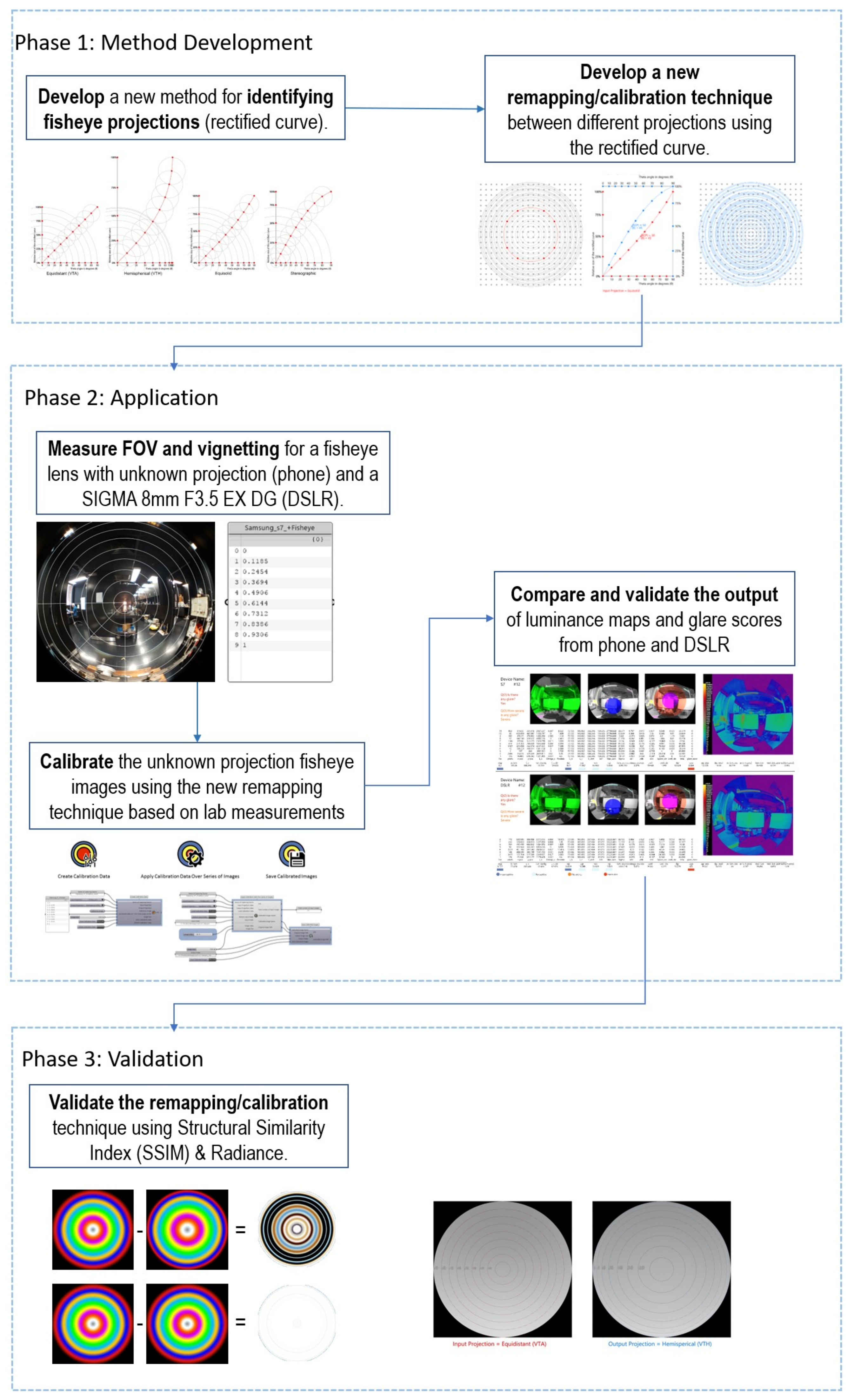
A manufactured fisheye lens can never truly conform to a theoretical symmetrical radial projection—a non-linearity that has been acknowledged but not addressed. The closest would be Cauwerts and Bodart [13], whose main aim was to develop a generalized vignetting function, but observed the radial symmetry between two SIGMA 4.5 mm F2.8 equisolid fisheye lenses mounted on two Canon 40D cameras. They developed a theoretical mapping function to approximate the lens projection to the mathematical equisolid angle projection based on observing the radial tendency in an experimental study.

However, fisheye lenses have different projections, depending on the manufacturer. Generally, there are four known mathematical projections: equisolid, equidistant, hemispherical and stereographic, all of which are differentiated by their Theta angle (altitude) (see Figure 1) and serve different purposes in photometry.

In the case of glare analysis, the equidistant projection is most used because it equally distorts objects at the center and the periphery. Both the equidistant and hemispherical projection are supported by glare evaluation tools like Radiance and Evalglare. To date, there is no simple method for correcting the projection distortion for fisheye lenses specific to glare analysis. Although in the areas of geometric computer vision and photogrammetry, researchers have developed algorithms to transform fisheye projections. For example, Kannala and Brandt [20] proposed a generic camera model to correct fisheye lens distortion using planar checker patterns photographed at different angles. Their approach was to take an equidistant projection and transform it onto a planar projection (see Figure 2). A parametric mathematical formula was developed to correct the radial and tangential image distortion using known control points in MATLAB. It was also proposed that the generic model could address over-fitting issues or be extended to suit fisheye projections wider than 180°. However, the final output of their method is not suitable for glare analysis because it does not remap the fisheye image to an equidistance or a hemispherical projection.

For glare analysis, the algorithm must correct the projection distortion in order to extract and calibrate luminance maps from HDR images. The projection transformation must therefore account for the luminance distortion caused by the image projection; which is most dominate at the periphery [13]. Furthermore, to make the HDR image useful for glare analysis, the projection must be transformed into the appropriate projection type which needs to be accurate to the pixel level. Unless specified by the manufacturer, the fisheye lens’ projection would be unknown.

Since all previous efforts were focused on removing the distortion and converting fisheye images into projective pinhole models using free tools such as panorama tools [21], the final output of these methods would not be suitable for glare analysis. These methods cannot be used to remap the fisheye image into circular fisheye image with an equidistance or a hemispherical projection in order to calculate luminance information at the pixel level accuracy. To this end, this paper presents an original contribution by proposing a standardized calibration procedure for glare analysis by addressing these two issues: (a) correcting projection distortion and (b) transforming the unknown projection to one of the commonly used projections in glare analysis.

3. Methodology

A methodology was developed involving three major phases, as shown in Figure 3. The first phase was the development of a geometrical model to identify the fisheye projection type and to perform a projection remapping. In this paper, the corrected image projection was defined by the rectified projection of Theta angles to achieve a pixel by pixel precision. The second phase included an application of the new remapping method for the fisheye lens with the unknown projection. A 190° equisolid SIGMA 8 mm F3.5 EX DG fisheye lens mounted on a Canon 5D camera, and a 195° fisheye commercial lens with an unknown projection, mounted on the rear camera of a Samsung Galaxy S7 (Figure 4) were used to develop and test the methodology. A comparative analysis was made between the two devices using glare scores. The final phase validates the remapping method using a structural similarity index (SSIM).

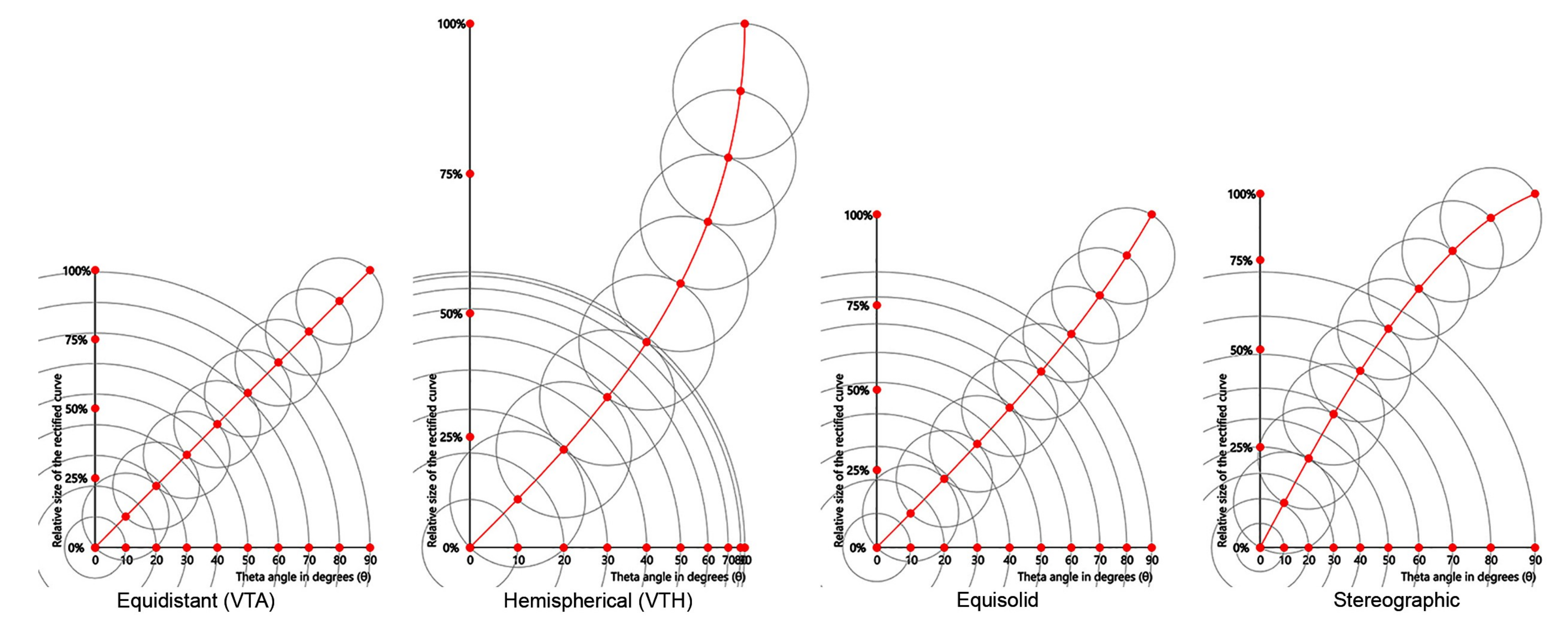
3.1. Phase 1: A New Method for Defining and Remapping Fisheye Projections

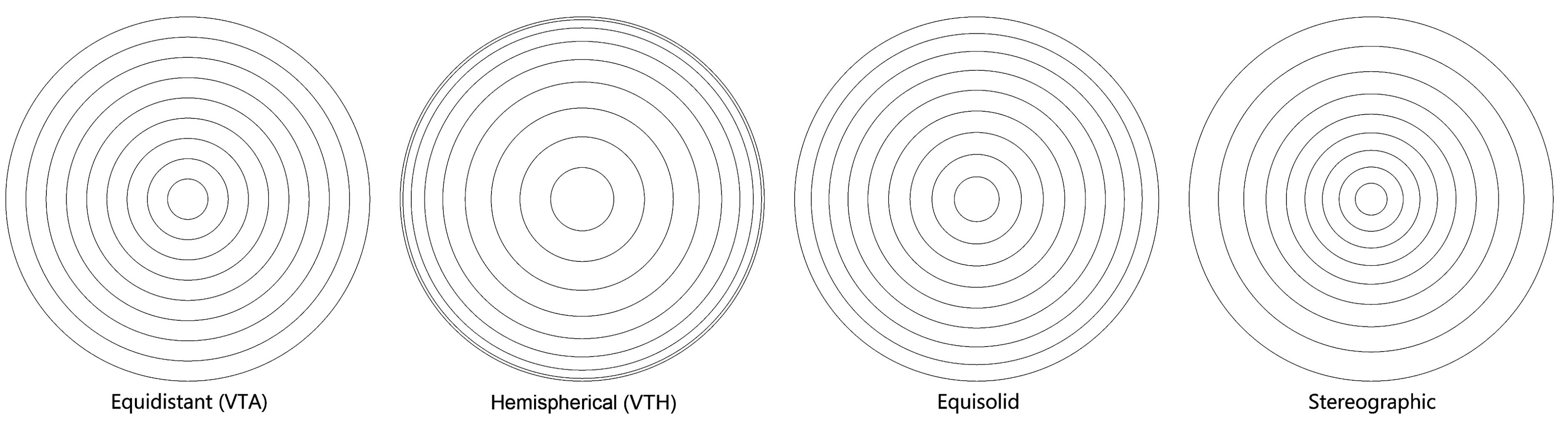
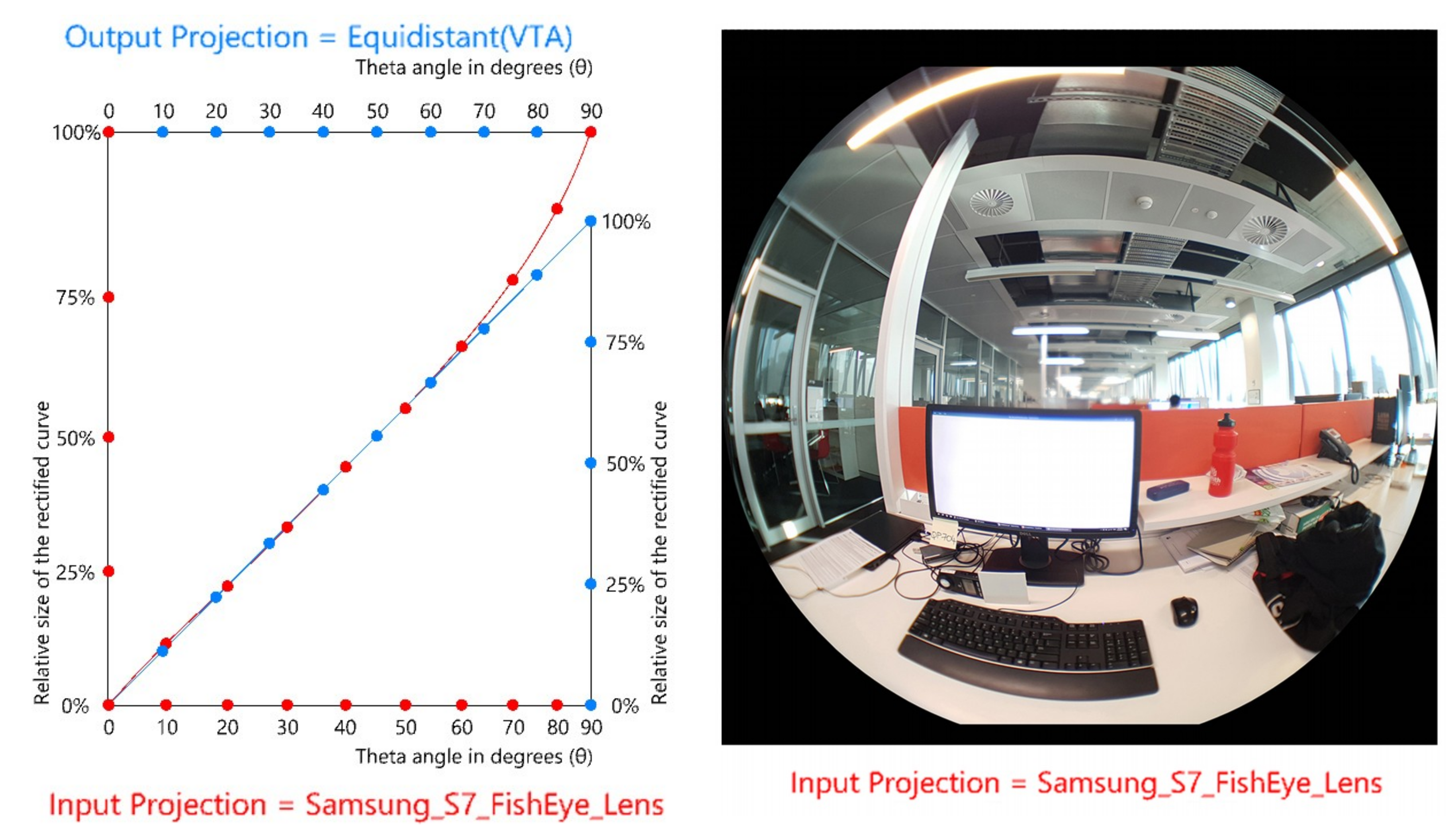
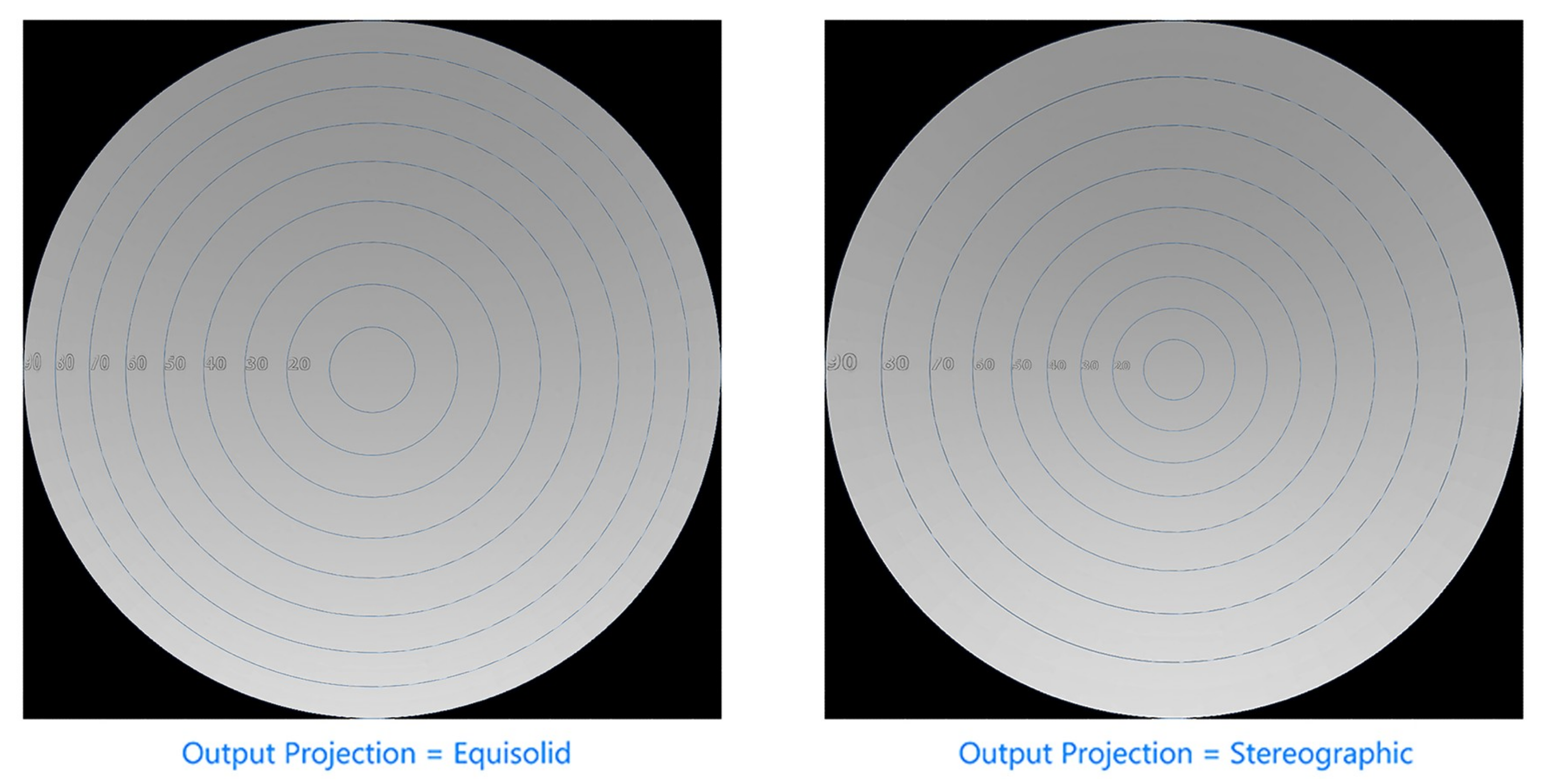
3.1.1. Defining Fisheye Projections (Rectified Curve)

A parametric geometrical model was developed to redefine the projection of fisheye LDR images, whereby a 180° hemispherical FOV was mapped to generate a rectified curve. In this study, the rectified curve was defined as a projection curve of θ angles of equalized segments between angles. Each projection has a unique rectified curve that can be identified. First, projection rings at 10° increments were created from 0° to 90° to represent Theta angles (θ). This was repeated for each projection type: equidistant (VTA) (1), equisolid (2), hemispherical (VTH) (3), and stereographic (4). Each projection was generated based on its theoretical formula [22]:

R = f × θ

(1)

R = f × sin (θ)

(2)

R = 2 × f × sin (θ/2)

(3)

R = 2 × f × tan (θ/2)

(4)

where R is the radius of the circle from the optical axis of the lens, f is the focal length, and θ is the angle measured from the optical axis. Each projection type is unique and can be visually distinguished by the radial distances as previously illustrated in Figure 1. A rectified curve can be developed for any projection type as shown in Figure 5, which enable transforming the fisheye image into a different projection type(s) and correcting the distortion issues. After creating the projection rings, a line along the X axis starting from the optical axis of the lens (the centroid of the fish-eye image) was drawn to intersect with each projection ring. This formed a list of intersecting points that represented the distance of each projection ring (from 0° to 90°) as shown in Figure 5a (referred to as Horizontal Curve or Curve A). The distance between each segment of the Horizontal Curve was ranked to select the biggest value. This was multiplied by 1.05% (which will be referred as Cr) to draw a small circle from the center of the image. A ray in the Y axis was drawn from the second point of Curve A (which represented θ of 10°), until it intersected with the circle. This generated the second point of the rectified curve; as the first point was the centroid of the image. From the second point, a new circle with the same radius as Cr was created to intersect with the ray at the third point of Curve A (representing θ of 20°). This process was repeated until the 10 points were defined as illustrated in Figure 5d. A Non-Uniform Rational Basis Spline (NURBS) interpolated curve was drawn through each point to create the rectified curve to represent the hemispherical projection (Figure 5e). From this, the same process can be used to generate a unique rectified curve for each projection type as shown in Figure 6.

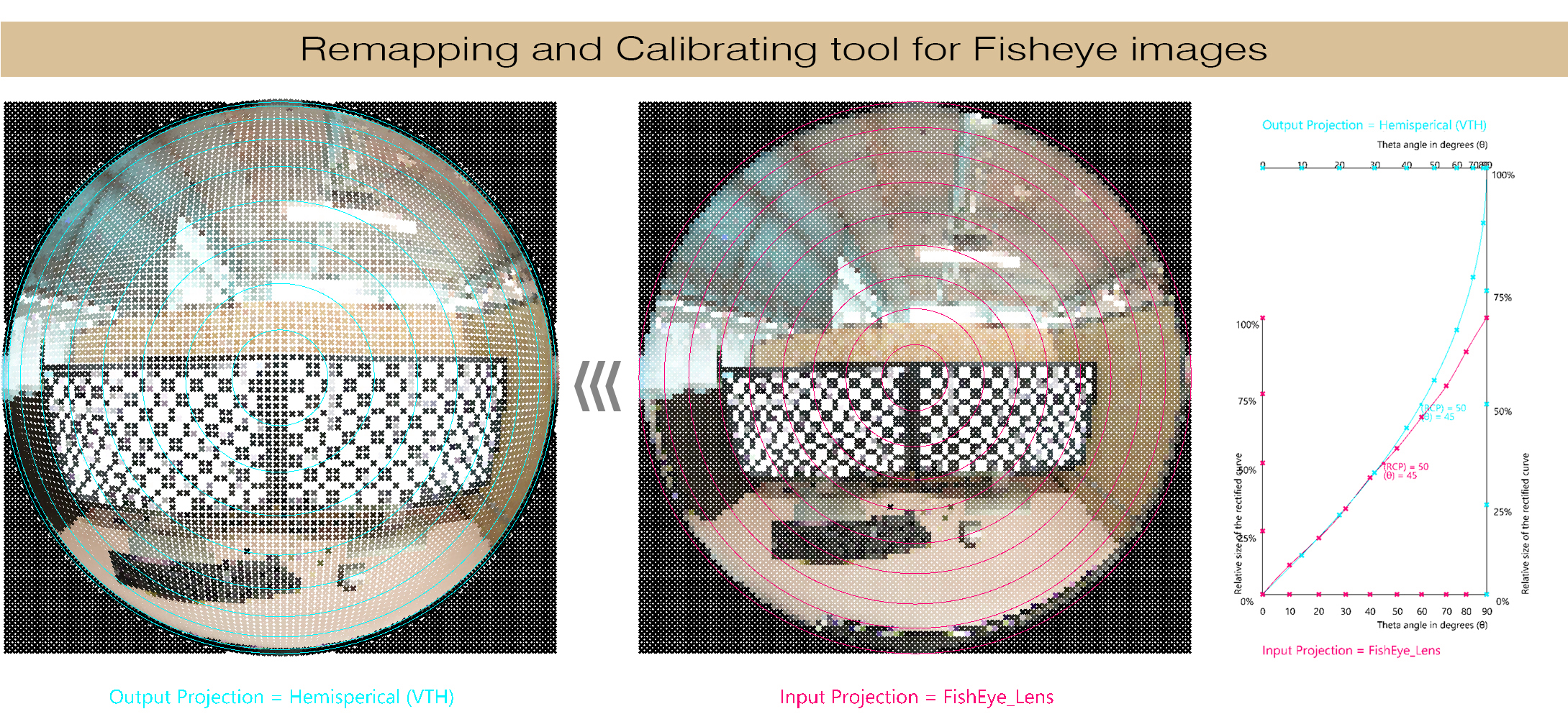
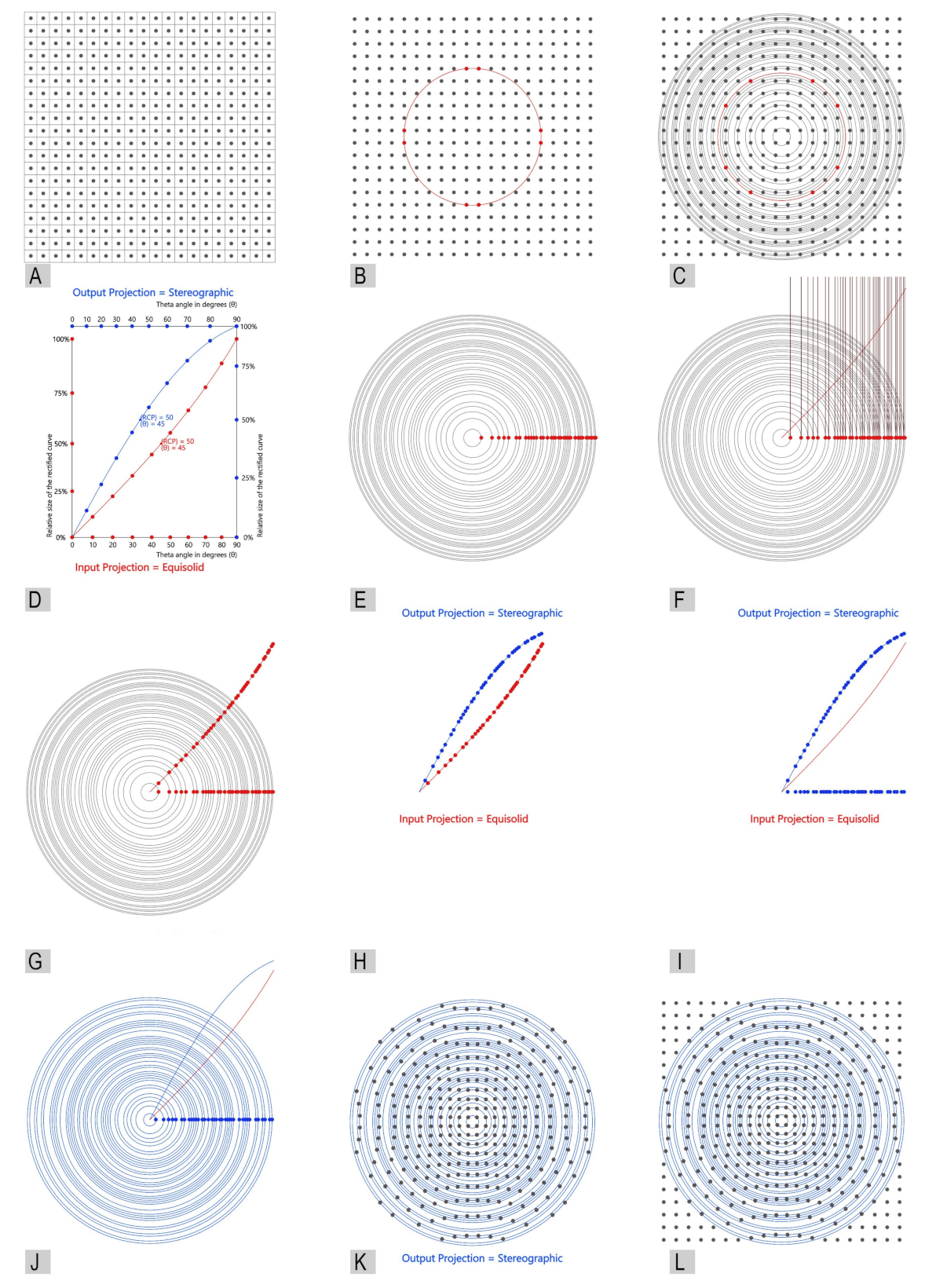
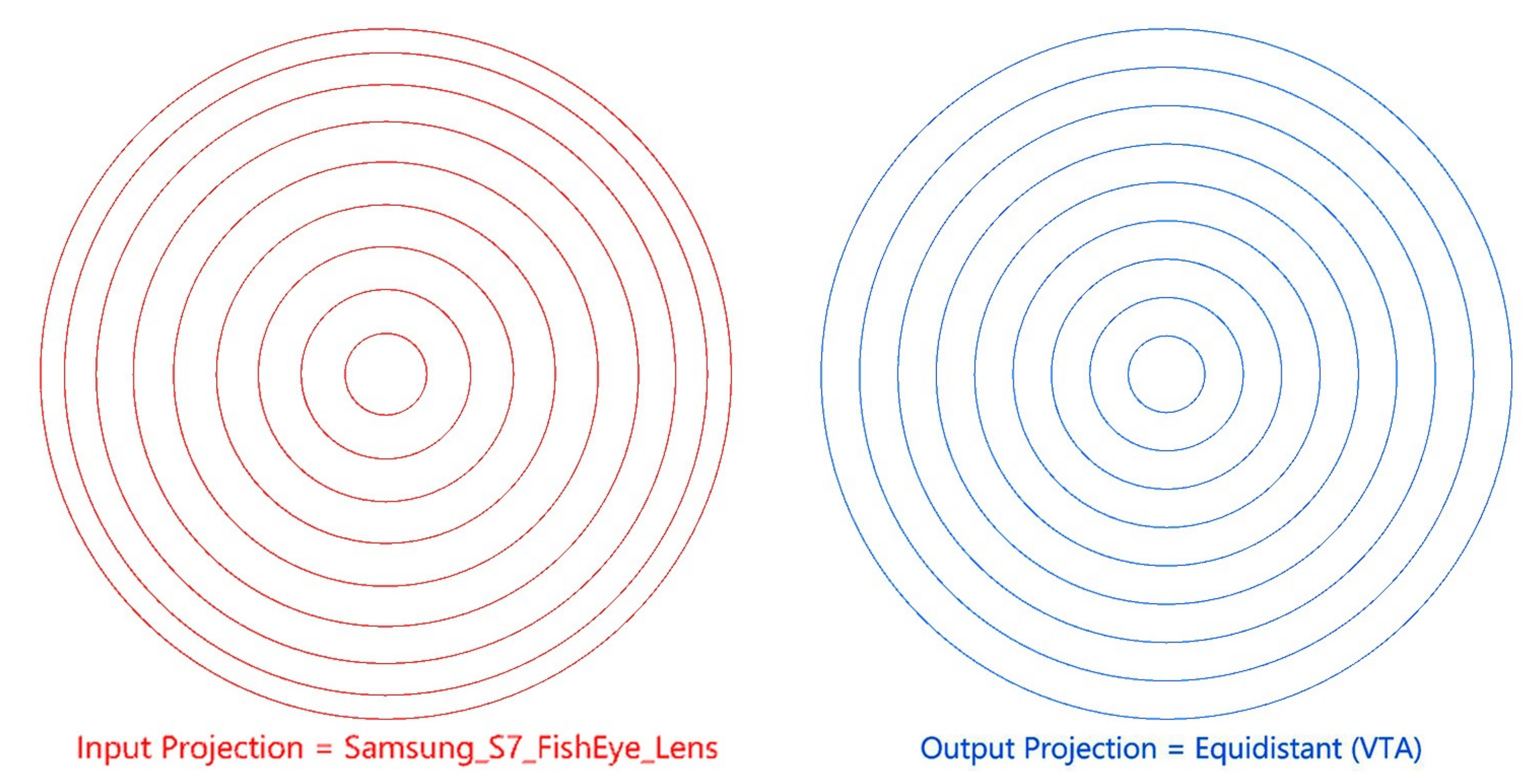
3.1.2. New Method for Remapping Fisheye Projections

The generated rectified curve was used as the reference projection to accurately transform a projection from one to another type. When fisheye images are imported, they are transformed into 2D pixelated grids (see Figure 7A for a simplified illustration image pixilation). To control each pixel in order to transform the fish-eye image into the corrected projection type, Cartesian coordinates were used and transformed into polar coordinates as illustrated in Figure 7B. The coordinates generated a series of projection rings using the same center point (see Figure 7C). Pixels (controlled by the polar coordinates) that shared the same circumference were grouped to reduce the amount of projection rings created in the process. These projection rings represented Theta angles (θ) from 0° to 90°. To transform the pixels onto a new projection type (assuming from equisolid to stereographic projection), the rectified curve was used to remap the pixels (described in Stage 1—see Figure 7D). First, the pixels were transformed into 3D points with X coordinate set equal to the radius of the circles. The Y and Z coordinates were set to zero. This generated a series of points on the X axis as shown in Figure 7E. These points were projected along the Y axis to intersect with the rectified curve, to define the original projection type of these points (see Figure 7F,G).

New points generated from the intersection inherited a new location parameter, which was defined as the percentage of the length of the rectified curve from 0 to 100%. By using the rectified curve, the points’ location was transformed from one curve to another based on the location parameter. For example, in Figure 7D the rectified curve shown in red has a point located at 50% that represented the Theta angle of 45° of the equisolid projection. To transform this to a stereographic projection (as shown in blue), a new point can be generated to represent the same Theta angle using the parameters of the equisolid curve based on its percentage length (50%). Similarly, all red points on the first curve were remapped to the blue curve creating the new blue points as shown in Figure 7H. These new points from the blue curve was projected back onto the X axis (see Figure 7I).

The X coordinate of the projected points produced a new radius of circles for the second projection that represented the same Theta angle as the first projection, as shown in Figure 7J. The relative location of the image pixels to the circle was retrieved to represent the new projection based on displacement of the circles (see Figure 7K). Finally, the points outside the circle boundary (the black colored points) were added to recreate the square image again as shown in Figure 7L. Then, k-Nearest Neighbor (k-NN) algorithm [23,24] was used to construct the new image.

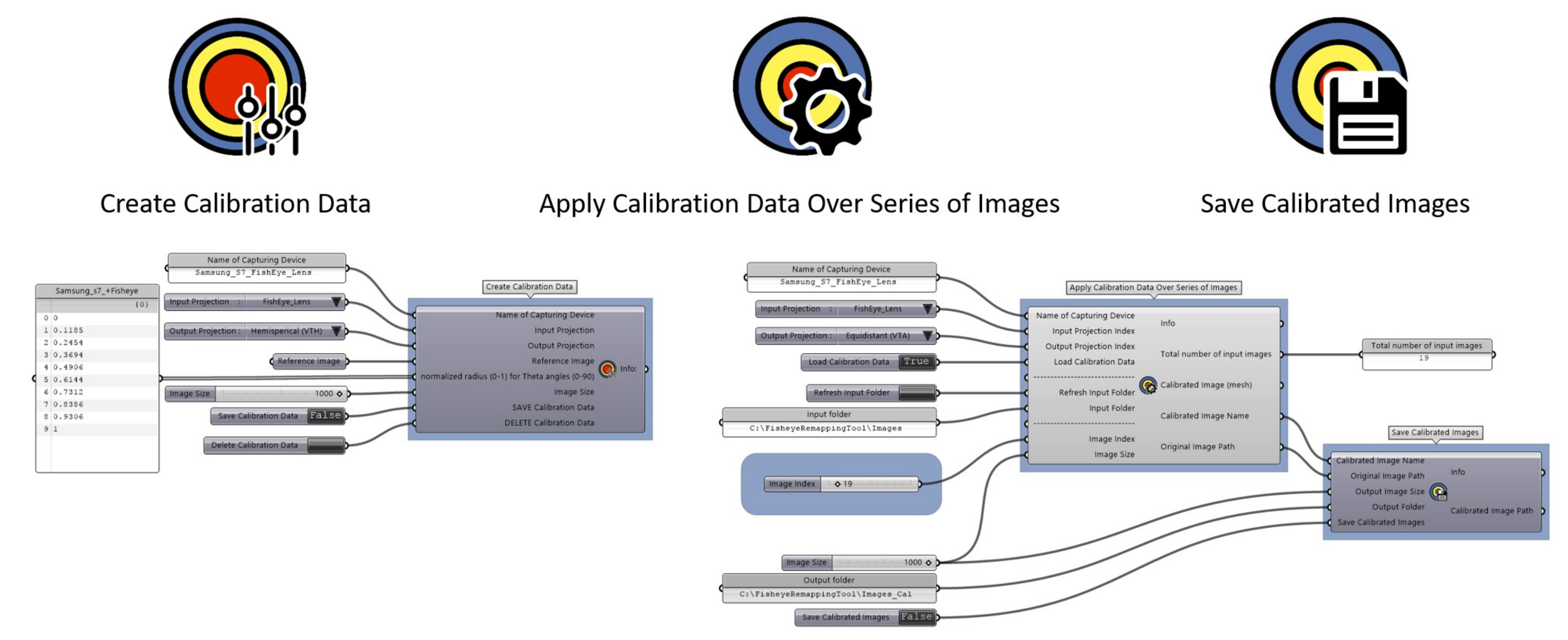
3.1.3. Developing Fisheye Remapping Tool

In recent years, there has been dramatic increase in employing Grasshopper [25] with daylighting, glare simulation as well as per-pixel post-processing applications [26,27,28,29,30]. Grasshopper is a 3D parametric modelling extension plug-in for Rhinoceros. Since it can provide real-time feedback to develop and test different algorithms [31], it was used to develop the remapping method. The methodology has been provided as an algorithm which can be used as a plugin within Grasshopper called Fisheye Remapping Tool. The developed tool can be accessed through the following link: [https://www.aymanwagdy.com/fisheyeremapping]. Fisheye Remapping Tool has been coded into three Grasshopper components as shown in Figure 8. The first component sets the input and output projection type(s). This component receives the fisheye images and generates the output projection by defining the normalized values of each projection ring which is explained in the following Section 3.2.1 Laboratory measurements procedure. The geometrical calibration data is created also by the first component and is saved as a layer in Rhinoceros. The second component loads the calibration data and collects the LDR images that need calibration. Then, the last component carries out the geometrical calibration for the images then copies the metadata information from the original images and store it with the calibrated images.

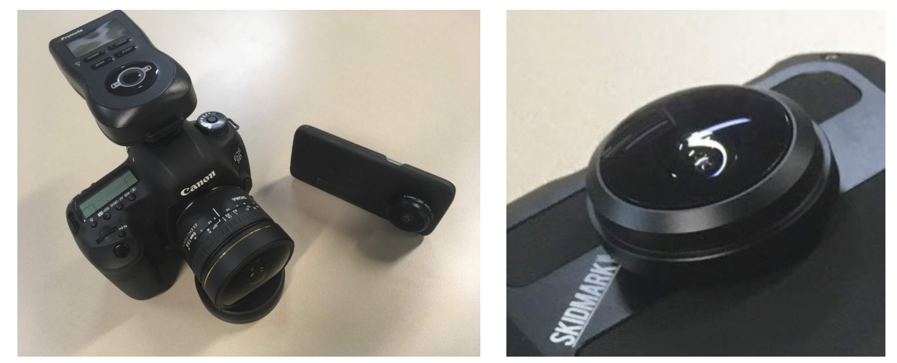
3.2. Phase 2: Application of the New Remapping Method for Physical Fisheye Lens

All previous steps were completed to provide a remapping method using predefined mathematical and geometric models for each projection type. However, the main contribution of this method is to develop an adoptable method that can be readily customized to calibrate and remap fisheye images for glare analysis. Usually, the issue with using a fisheye lens in combination with a DSLR camera or a smart phone, would require defining the photometric image projection, correcting the distortion resulting from the fisheye lens, accurately cropping the photometric image to a 180° FOV and, correcting the vignetting. Any of these issues can affect the reliability of the luminance information of an HDR image. Thus, it is crucial to know and calibrate the image projection type of the fisheye image and to remap these images onto an equidistance projection for glare analysis. Therefore, the following measuring procedure generates similar input data such as the one achieved with the geometrical model created in phase 1 (in which a new rectified curve for camera’s lens can be created). As a result, the fisheye images can be calibrated and remapped in preparation for glare evaluation.

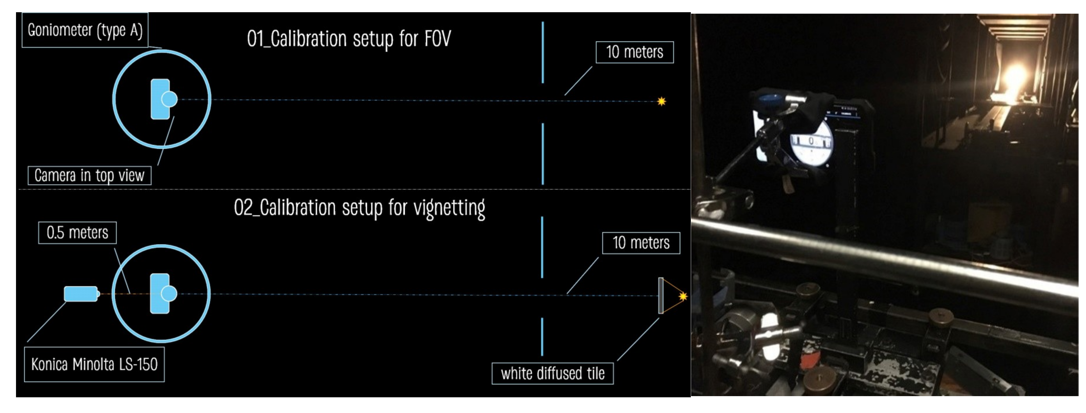
3.2.1. Laboratory Measurements

Physical measurements were conducted in a laboratory tunnel room using a Goniometer (type A). Calibration setup was prepared to measure the 180° FOV from the two fisheye lenses and determine the vignetting effect of two chosen devices: a DSLR camera, and a Samsung Galaxy S7. Measurements were standardized by aligning the center point of each fisheye lens to an incandescent lamp (light source positioned 10 m away) using a laser beam. An internal accelerometer and the gyroscope sensors (a feature within the Samsung Galaxy S7) were used to remove inclination along the axes. Both fisheye lenses were aligned to the center point of the fisheye lens to the center point of the light source. The lamp was placed at a maximum distance of 10 m to reduce angular measurement errors while rotating the Goniometer. The measurement procedure was repeated twice, one with direct view of light source and one with a white diffusing filter for measuring the FOV and the vignetting effect respectively, as shown in Figure 9. This filter was placed in front of the lamp to diffuse the light source and create an even distribution of light. Spot luminance measurements were taken of the filter using a luminance meter (Konica Minolta LS-150) before, during and after images were captured from each device. The light meter was fixed on a tripod 0.5 m behind the capturing device and 0.1 m above the plane with the phone and the diffusing filter. The calculated angle between the measuring direction and the plane is 0.55 degrees. The light source was connected to a DC current supply and the voltage was monitored to ensure that the lamp was stable. The procedure for taking LDR images at different exposures was repeated at every 10° increment from 0° in the optical axis of the lens to 90° for the X (horizontal) Y, (vertical) and, Z (diagonal) axes (see

Table 1. Summary of camera settings for both devices.

Camera Settings
Exposure Time (Shutter Speed) Phone
1/24,000	1/16,000	1/8000		1/4000	1/2000	1/1000	1/500	1/250	1/125	1/60	1/30	1/15	1/8	1/4	1/2	1
Exposure Time (Shutter Speed) DSLR
1/8000	1/2000	1/500		1/125	1/30	1/8	1/2	2	8
ISO Phone			64
ISO DSLR			400
White balance:			daylight
Image quality:			*.jpg (max)
Color space:			sRGB
Focus:			infinity (auto is off)
Picture style:			standard

for summary of camera settings for each device).

This method created a circle at each Theta angle (projection ring) for the optical system of the fisheye lens, which can be used as the input data type to run the calibration algorithm. As expected, the projection rings of the 180° FOV of the fisheye commercial lens attached to the phone showed some distortion. The curve did not follow any of the mathematical models shown in Figure 10. A rectified curve was generated using Fisheye Remapping Tool, after which it became possible to calibrate and remap any picture taken with this configuration (smart phone with fisheye) to any of the mathematical fisheye projection types see Figure 11 and Figure 12.

3.2.2. Image Processing Procedure

The post-processing procedure was conducted using multiple software packages. Photoshop was used to create automated action to crop each LDRi to cover the 180° hemispherical view and resize the images to 1000 by 1000 pixels. Images were imported into Grasshopper to perform geometrical calibration using the Fisheye Remapping Tool. Although this tool can remap the phone images into any type fisheye projections as shown in Figure 11 and Figure 12, the images were remapped to equidistant projection since it is supported by glare analysis tools.

A Camera Response Function (CRF) was generated to compute the HDRi from each device following Mitsunaga and Nayar [12] CRF method and using multiple scenes to form one large HDR image. The HDR image was constructed following best known practice [14,32,33,34] and therefore includes a wide variety of luminance and color information (shown in Figure 13). To adjust the absolute luminance values of the HDRi, the luminance of a small defined area within the image was recorded (using a LS-100 Konica Minolta). Based on the ratio between the luminance value of the image and the measured value, the CRF calibration factor is calculated and applied to CRF to achieve accurate results. The calibrated CRF is saved as a pre-defined setting to generate the HDR images.

Vignetting calibration was conducted after the HDRi was computed. To derive this calibration, a camera vignetting curve was needed. This curve represented the light falloff within the FOV. A Grasshopper algorithm was developed to generate a vignetting curve to compute a calibration factor for each pixel (see Figure 14) which was exported as a CSV file. The algorithm used the luminous values taken from HDRi of the diffusing filter and compared it to spot measurement in order to calculate the calibration factors as shown in

Table 2. The relationship between the luminance of the diffusing filter calculated from HDRi and spot measurement.

Theta Angle (θ)	Luminance of Diffusing Filter	Loss Percentage	Calibration Factor
0	155	18.95%	1.23
10	165	13.73%	1.16
20	155.16	18.87%	1.23
30	171.14	10.52%	1.12
40	173.2	9.44%	1.10
50	153.96	19.50%	1.24
60	142.99	25.23%	1.34
70	127.31	33.43%	1.50
80	110.85	42.04%	1.73
90	51.2	73.23%	3.74

. MATLAB was used to multiply the CSV file with the HDR images to correct the vignetting effect of the lens.

The Grasshopper algorithm was coded as a tool and it is available through the following link: [https://www.aymanwagdy.com/fisheyevignetting].

Finally, the absolute luminance of the HDRi was calibrated by comparing the luminance value of a small defined area within the image to the value recorded by the hand-held luminance meter LS-100 Konica Minolta.

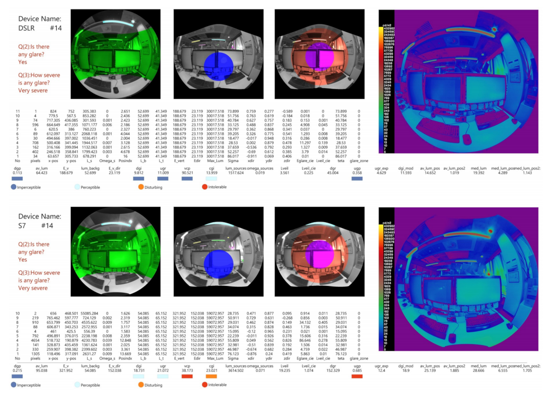
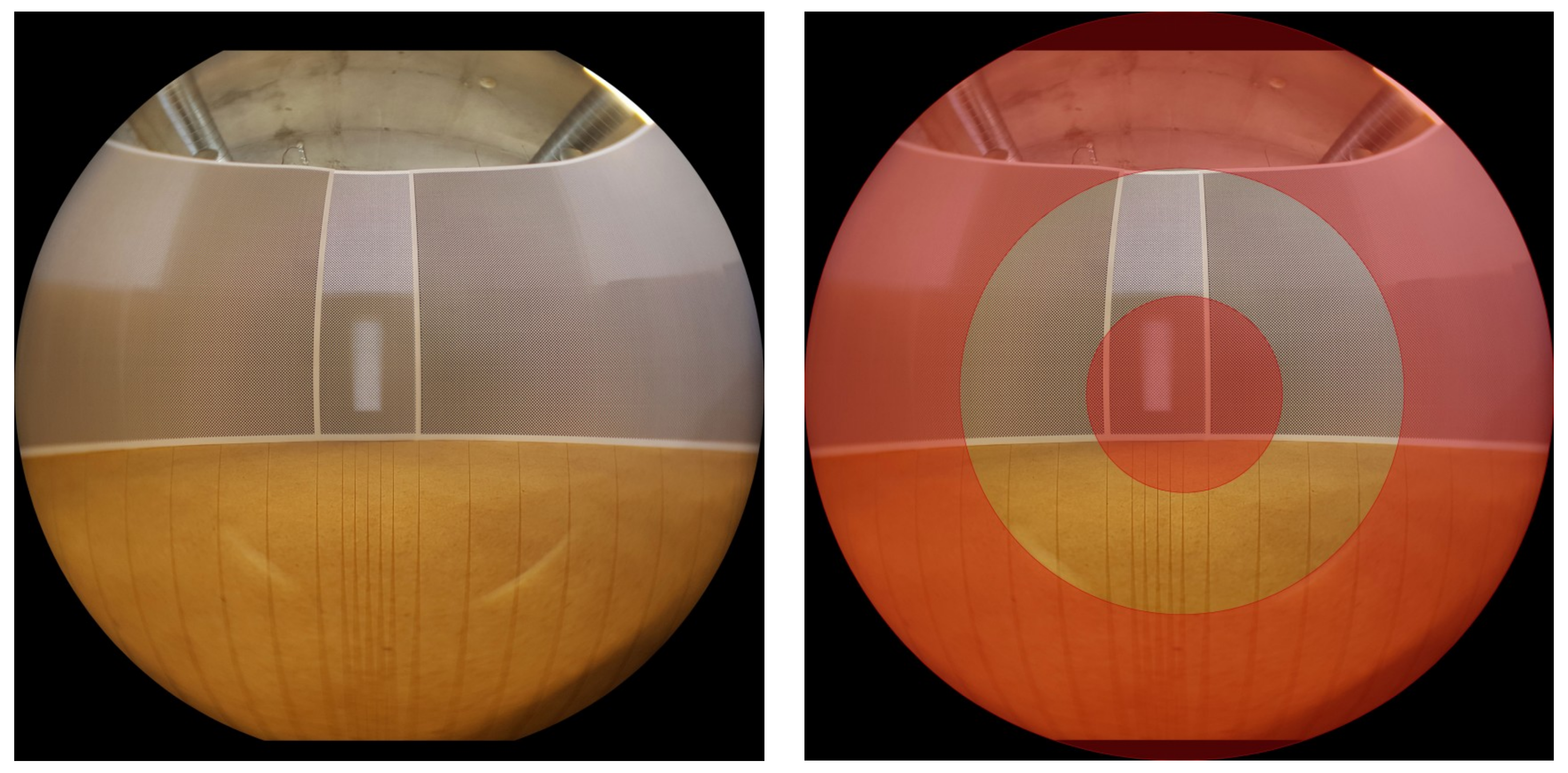
3.2.3. Glare Analysis

The previous calibration process was carried over 56 HDR images collected from three open-plan offices in a field study in Brisbane, Australia. The calibrated images were analyzed by Evalglare to extract the luminance information and to calculate different glare indices. Evalglare settings were adjusted to detect glare sources based on the task area method with a multiplying factor of 4 to evaluate visual scenes with contrast glare in accordance with Pierson, Wienold [35]. Results were evaluated through a statistical analysis in order to achieve two objectives. The first objective was to measure error percentage resulting from the use of non-calibrated images in glare analysis which emphasized the importance of conducting the calibration procedure. The second objective was to compare glare scores and luminance maps generated from Samsung Galaxy S7 and DSLR to demonstrate the validity of cameras from mobile phones as tools for image acquisition for glare analysis.

Glare scores of the 56 calibrated HDR images were statistically compared to non-calibrated versions of the same images. The minimum, maximum and the average difference in each glare score were recorded. Differences ranged significantly from one index to another, with averages ranging from 5% in av_lum_pos2 metric to 167% in DGI as shown in

Table 3. Glare score results: the percentage difference in values between the calibrated and non-calibrated images over 22 metrics.

Index	Max	Min	Average	Index	Max	Min	Average
DGP	20%	−54%	9%	Lveil	61%	−484%	61%
Av_lum	7%	−69%	13%	Lveil_cie	89%	−483%	58%
E_v	8%	−30%	7%	DGR	39%	−124%	17%
DGI	13%	−4609%	167%	UGP	19%	−284%	19%
UGR	19%	−282%	19%	UGR_exp	413%	−1547%	70%
VCP	56%	−128%	14%	DGI_mod	15%	−234%	16%
CGI	20%	−122%	11%	Av_lum_pos	3%	−34%	7%
Lum_sources	10%	−94%	14%	Av_lum_pos2	2%	−26%	5%
Omega_sources	25%	−217%	32%	Med_lum	−12%	−54%	6%
Lum_backg	18%	−31%	8%	Med_lum_pos	1%	−50%	7%
E_v_dir	26%	−444%	60%	Med_lum_pos2:	−6%	−47%	6%

. In general, results denote the underestimation of glare scores in non-calibrated images and emphasized the significance of calibration prior to glare evaluation.

Detailed glare analysis was conducted using Evalglare in which it returned twenty-two (22) values of luminance, illuminance and glare scores which were detailed in the Supplementary Materials. These analyses were carried out over the calibrated HDR images for each device. Statistical data analysis was used to examine the relationship between by the two devices. This was accomplished by computing the linear correlation and significance between each glare score as detailed in

Table 4. Glare score results: the correlation and the significance between DSLR and Samsung S7 over 22 indices.

luminance, Illuminance and Glare Metrics	Correlation	Sig. (2-Tailed)
DGP	0.887	p < 0.001
Av_lum	0.927	p < 0.001
E_v	0.981	p < 0.001
Lum_backg	0.861	p < 0.001
E_v_dir	0.979	p < 0.001
DGI	0.914	p < 0.001
UGR	0.886	p < 0.001
VCP	0.821	p < 0.001
CGI	0.878	p < 0.001
Lum_sources	0.564	p < 0.001
Omega_sources	0.951	p < 0.001
Lveil	0.973	p < 0.001
Lveil_cie	0.929	p < 0.001
DGR	0.768	p < 0.001
UGP	0.886	p < 0.001
UGR_exp	0.975	p < 0.001
DGI_mod	0.911	p < 0.001
Av_lum_pos	0.992	p < 0.001
Av_lum_pos2	0.993	p < 0.001
Med_lum	0.972	p < 0.001
Med_lum_pos	0.949	p < 0.001
Med_lum_pos2	0.957	p < 0.001

. Most of the indices -21 out of 22- showed high correlation up to (0.993). However, in some cases variations were found which were explained further in the discussion. One of the 56 scenes (see Figure 15) was used to compare luminance maps and glare scores between a DSLR camera, and a Samsung Galaxy S7. The luminance map scale was set to a maximum of 500,000 cd/m² with log 5 intervals in order to have a constant luminance scale. The HDRi was rendered into false color map using Radiance to generate luminance maps. As highlighted in Figure 15, the luminance disruption was almost similar between the two devices. However, when a very bright source was present in the FOV, the maximum luminance value reported by Samsung Galaxy S7 and DSLR was around 185,000 cd/m² and 1,024,000 cd/m². This happened due to the fixed aperture size of the mobile phone (F1.7). This limitation not only affected the brightness of all glare scores, but also changed the glare classification in some cases from one category to another. However, both devices identified the same glare sources and most of the glare scores were similar.

3.3. Phase 3: Validation

To test and validate the proposed remapping method, two validation tests were conducted. The first test evaluated the accuracy of the pixel remapping, while the second tested the color distortion.

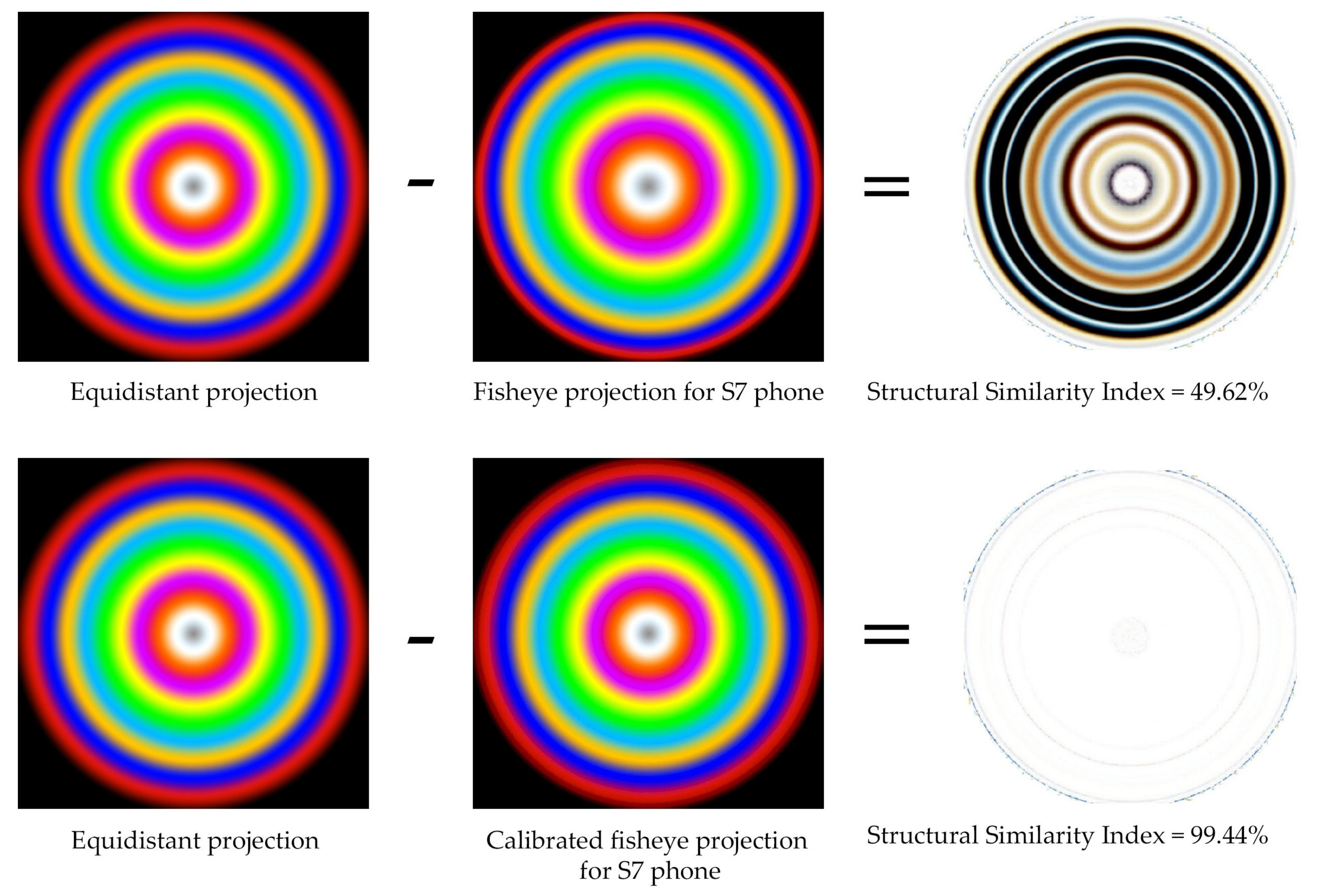
3.3.1. First Validation Test: Pixel Remapping

First, a fisheye image was rendered in Radiance [36] to create an image with accurate equidistance projection. This was used as a benchmark to compare with the new calibrated images from the algorithm. The rendered image has a corresponding Theta angle for each projection ring plotted in dark grey as shown in Figure 16.

The validation process started with importing the benchmark image to the algorithm and was defined as an equidistance fisheye 180° image. This generated red circles that overlaid the image in Grasshopper. In this instance, these red rings represented the mathematical model of equidistance projection; which precisely overlaid with the grey circles of the benchmark image. This indicated that the radiance image had accurate projection, as expected. To validate the remapping process quantitatively, MATLAB was then used to calculate the difference between the projection rings by measuring and comparing the radius of each circle found in the benchmark image and the expected correct value calculated from the mathematical model.

The accuracy of this algorithm in remapping fisheye images from one projection to another was tested by overlaying the mathematical model of the desired projection on top of the new remapping benchmark image. This was done by checking the differences between the projection circles of the mathematical model and the Radiance image. As the hemispherical image projection has strong distortion near the circumference, it was used to test the accuracy of this tool. After the desired output projection was set to hemispherical, the blue circles, which represents the mathematical model of hemispherical projection, overlaid precisely over the grey circles of the new transformed image as illustrated in the left picture of Figure 17. This was also confirmed by measuring the differences between the circles in MATLAB. Moreover, Different output images were tested, including the equisolid angle and stereographic projection, with the same accuracy in mapping results, as shown in Figure 18.

3.3.2. Second Validation Test: Color Distortion

To measure the color distortion resulting from the remapping process and to evaluate the image quality, Structural Similarity Index (SSIM) metric was used [37]. This metric uses an error sensitivity approach to decompose the image and estimate the visible errors between two images. Figure 19 shows the two test configurations. The test was carried out by comparing two gradient-colored images: one with original equidistant projection and one with actual projection of fisheye lens of S7 mobile. The SSIM index was 49.62%, which means that more than half of the image is misaligned with equidistant projection. The second test used a calibrated fisheye image based on the developed method and compared it with the original equidistant image as shown in Figure 19. Structural Similarity Index indicated 99.44% similarity between the images. It is apparent from SSIM image that very few pixels were showing errors around the periphery. These errors in color were a result of a stretching phenomenon that accrues around the periphery when the image is deformed from one projection to another.

4. Discussion and Limitations

This paper presents a methodology for calibrating and remapping fisheye projection(s) for glare analysis. A geometrical model was used to correct the projection distortion, and to transform this from one projection to another (i.e., equidistant, equisolid angle, orthographic or stereographic) using three phases. For correct luminance assessment and luminance mapping, angular projection needs to be accurate down to the pixel level. That is why an exact fitting was intended in our calibration method, as it defined the projection distortion of the fisheye lens. If a simplified curve is used, it will not yield an accurate remapping from one projection to another. This can be confirmed using the Structural Similarity Index (SSIM) test, which will indicate a large percentage error similar to Figure 19. Therefore, we modeled a 2D curve using Rhino3D, which is 3D Non-Uniform Rational B-spline (NURBS) software for generating B-splines, in order to connect the 10 projection points, as shown previously in Figure 5 and Figure 6. This method was combined into an easy to use plugin that can be used within parametric modelling software such as Grasshopper.

After introducing the geometrical model for remapping the fisheye projections in phase one, laboratory measurements were carried out to apply this method on HDR images generated from two fisheye lenses mounted on DSLR and smart phone camera. Using the proposed method, 56 HDR images were calibrated by correcting projection distortion, vignetting, and luminance error. In the last phase, the method was validated through two tests: accuracy of pixel remapping and color distortion. The results showed that this method is accurate, efficient and reliable as a post-processing technique for correcting distorted projections from fisheye images and for remapping projections. Furthermore, it was possible to define lenses of unknown projections and remap them to any other projection (e.g., equidistant) to be suitable for glare analysis. This enables researchers to recover distorted images in field research and make the use of smart phones and/or cameras a reliable method to capture the luminous environment.

By comparing calibrated versus non-calibrated images through 22 glare indices, statistical analysis showed the significance of the calibration procedure to avoid significant errors in glare analysis. The same image data were used to examine the reliability of smart phone camera compared to DSLR camera for image capturing for glare analysis. There was a high correlation between the two devices, as the same glare sources were identified, and glare scores were similar. However, some cases seemed to be non-linearly related. This is due to two important factors that caused variation between the output of the two devices (DSLR and calibrated phone):

(1)

The maximum luminance reading that can be captured with the device due to hardware limitation, and

(2)

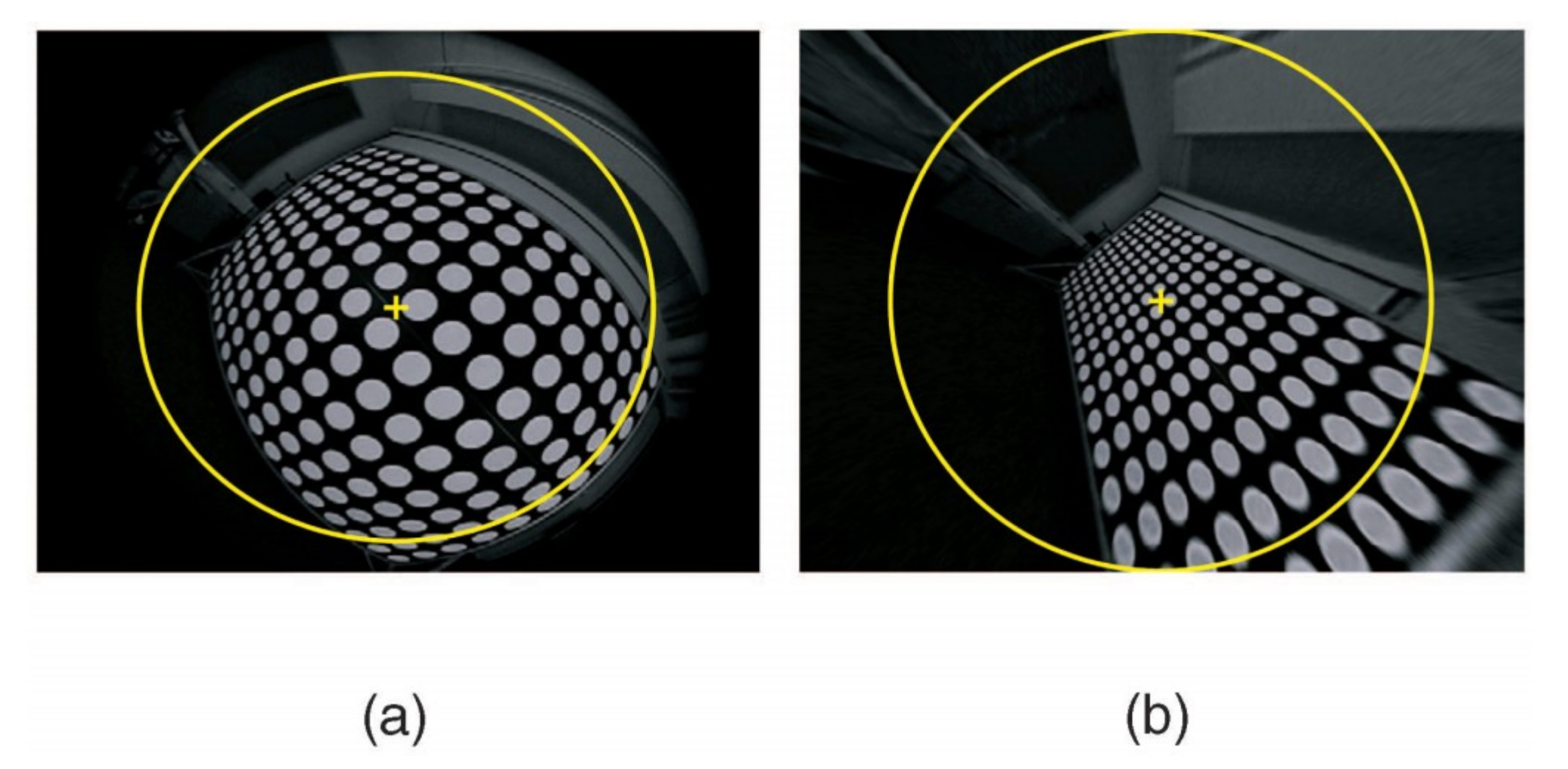
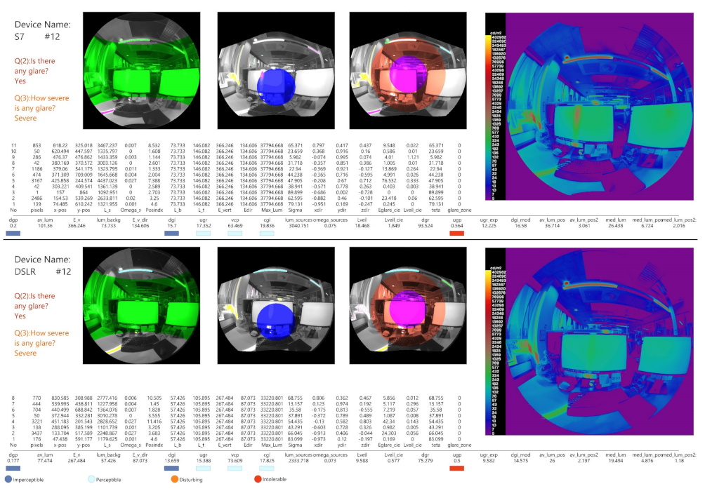
The limitation of taking the same field of view in both devices; since we had 10 cm gap between them, each device had a slightly different FOV. In some cases, the main glare source was shaded in one of the two captured images, as shown in Figure 20, which caused random errors.

The key advantage of using a mobile camera is the electronic shutter speed, which can reach high speeds of up to 1/24,000 s (as found for the Samsung S7). Although the electronic shutter outperformed the mechanical shutter speed, which topped out at 1/8000 s, the aperture size for mobile phones is usually fixed to a large value (2.2 or lower), which increases the amount of light that reaches the camera sensor. As a result, mobile phones produce brighter images than the DSLR, even with the maximum shutter speed selected in both devices. This hardware limitation confines the accuracy of mobile phones to identify the luminance values of very bright sources. A quantification of this problem was found in the maximum luminance value reported based on 56 HDR images (185,000 cd/m²) for the Samsung S7 smartphone and (1,024,000 cd/m²) for the DSLR camera. However, further studies will be conducted to investigate this limitation and possible solutions in future studies.

In addition, we found that the large aperture size of the built-in lens of the phone made it challenging to adjust the image focus. Since the fisheye lens was mounted in front of a wide-angle lens of the phone, the combined optical properties of the two lenses blurred some regions of the image even after setting the focus to infinity. This resulted in distortion of luminance intensity in these regions, as shown in Figure 21. It was found that the vignetting calibration corrected the luminance distortions, yet the image quality still showed blurred areas. This limitation did not apply to the DSLR camera with the fisheye lens.

The new projection curve of the phone was compared to the mathematical fisheye projection curves. It was found that the curve is a kind of deformed version of equidistant angle projection. As illustrated in Figure 10 the new curve starts to deviate from the mathematical model of equidistant projection at 30 degrees and onwards, which affects the size of any potential glare source located between 30 and 90 degrees.

While developing this method, the existing literature reported that the SIGMA 8 mm F3.5 EX DG fisheye lens uses an equidistant projection, our measurements indicated that it has an equisolid angles projection type, which was confirmed as well by the Photolux provider who distributed the pre-calibrated DSLR cameras with fisheye lens.

5. Conclusions

This study provided a new remapping method for glare analysis through defining and remapping fisheye projections through a geometrical model which was then validated through laboratory measurements. The algorithm of this method was transformed into a friendly user interface tool through Grasshopper. We believe this fisheye remapping and calibration tool will aid researchers in working with fisheye images and will give them the flexibility to change between projections systems with high level of accuracy.

The developed method resolved the issue of using fisheye lenses of unrecognized image projections. The model can transform any LDR image even with any projection to a recognized projection that can be used in glare evaluation tools. This tool allowed the use of any image projection for glare analysis without concerning about the limitations of glare evaluation tools such as Evalglare of accepting only equidistant or hemispherical image projections. The proposed method was validated using two methods; first, a fisheye image rendered in Radiance that acted as a benchmark for new calibrated images from the algorithm and it precisely coincided with it when measure in MATLAB. The second validation test was carried out using the Structural Similarity Index (SSIM) metric to compare visible errors in fisheye projection before and after calibration in relation to the accurate equidistant projection of the same image, which indicated 50.38% and 0.56% respectively.

The vignetting calibration was also addressed by this study, which is inherently caused by fisheye lenses, by identifying the magnitude of luminance loss and calculating the calibration factor at each Theta angle to compensate this loss. This was done through lab measurements where we calibrated the vignetting of two devices (smart phone Samsung S7 and DSLR camera) by capturing a series of HDR images at 10 degree increments.

Fifty-six (n = 56) HDR images collected from three open-plan offices in a field study were used to compare glare output of smart phone Samsung S7 and DSLR camera. Evalglare was used to calculate 22 glare, luminance and illuminance indices where the linear correlation was computed to find the correlation between the two devices which in some indices ranged between (0.768) to (0.993) except the luminance of the source index. Although the maximum luminance value reported—based on 56 HDR images—by the smart phone (185,000 cd/m²) was lower than the DSLR camera (1,024,000 cd/m²), the same glare sources were identified, and most glare scores were similar, since we used the task luminance method (glare sources were identified when the luminance of the glare source is 4 times higher than the average luminance of the task).

Finally, based on the high correlation between DSLR and Samsung S7 with 21 out of 22 indices and high accuracy of the calibration process of 99.44%, we confirm the reliability of using smart phones in capturing HDR images for photometric and glare research if the camera setting was adjusted according to Table 1.

References

1. Tzempelikos, A. Advances on daylighting and visual comfort research. Build. Environ. 2017, 100, 1–4. [Google Scholar] [CrossRef]
2. Jacobs, A. High dynamic range imaging and its application in building research. Adv. Build. Energy Res. 2007, 1, 177–202. [Google Scholar] [CrossRef]
3. Jacobs, A.; Wilson, M. Determining lens vignetting with HDR techniques. In Proceedings of the XII National Conference on Lighting, Varna, Bulgaria, 10–12 June 2007. [Google Scholar]
4. Hirning, M.B.; Isoardi, G.L.; Cowling, I. Discomfort glare in open plan green buildings. Energy Build. 2014, 70, 427–440. [Google Scholar] [CrossRef]
5. Hirning, M.B.; Isoardi, G.L.; Coyne, S.; Garcia Hansen, V.R.; Cowling, I. Post occupancy evaluations relating to discomfort glare: A study of green buildings in Brisbane. Build. Environ. 2013, 59, 349–357. [Google Scholar] [CrossRef]
6. Konis, K.; Lee, E.S.; Clear, R.D. Visual comfort analysis of innovative interior and exterior shading systems for commercial buildings using high. resolution luminance images. Leukos 2011, 7, 167–188. [Google Scholar]
7. Borisuit, A.; Scartezzini, J.-L.; Thanachareonkit, A. Visual discomfort and glare rating assessment of integrated daylighting and electric lighting systems using HDR imaging techniques. Archit. Sci. Rev. 2010, 53, 359–373. [Google Scholar] [CrossRef]
8. Kurnia, K.A.; Azizah, D.N.; Mangkuto, R.A.; Atmodipoero, R.T. Visual comfort assessment using high. dynamic range images under daylight condition in the Main Library Building of Institut Teknologi Bandung. Procedia Eng. 2017, 170, 234–239. [Google Scholar] [CrossRef]
9. Wienold, J.; Christoffersen, J. Evaluation methods and development of a new glare prediction model for daylight environments with the use of CCD cameras. Energy Build. 2006, 38, 743–757. [Google Scholar] [CrossRef]
10. Nazzal, A.A.; Chutarat, A. A new daylight glare evaluation method. Archit. Sci. Rev. 2001, 44, 71–82. [Google Scholar] [CrossRef]
11. Hirning, M.B.; Isoardi, G.L.; Garcia-Hansen, V.R. Prediction of discomfort glare from windows under tropical skies. Build. Environ. 2017, 113, 107–120. [Google Scholar] [CrossRef]
12. Mitsunaga, T.; Nayar, S.K. Radiometric self calibration. In Proceedings of the 1999 IEEE Computer Society Conference on Computer Vision and Pattern Recognition (Cat. No PR00149), Fort Collins, CO, USA, 23–25 June 1999. [Google Scholar]
13. Cauwerts, C.; Bodart, M.; Deneyer, A. Comparison of the vignetting effects of two identical fisheye lenses. Leukos 2012, 8, 181–203. [Google Scholar]
14. Inanici, M. Evaluation of high dynamic range photography as a luminance data acquisition system. Lighting Res. Technol. 2006, 38, 123–134. [Google Scholar] [CrossRef]
15. Goldman, D.B. Vignette and Exposure Calibration and Compensation. IEEE Trans. Pattern Anal. Mach. Intell. 2010, 32, 2276–2288. [Google Scholar] [CrossRef] [PubMed]
16. Garcia-Hansen, V.R.; Cowley, M.; Smith, S.S.; Isoardi, G. Testing the accuracy of luminance maps acquired by smart phone cameras. In Proceedings of the CIE Centenary Conference “Towards a New Century of Light”; Commission Internationale l’Eclairage: Paris, France, 2013; pp. 951–955. [Google Scholar]
17. Sahin, C. Comparison and calibration of mobile phone fisheye lens and regular fisheye lens via equidistant model. J. Sens. 2016, 2016, 9379203. [Google Scholar] [CrossRef]
18. Debevec, P.E.; Malik, J. Recovering high dynamic range radiance maps from photographs. In ACM SIGGRAPH 2008 Classes; ACM: Los Angeles, CA, USA, 2008; p. 31. [Google Scholar]
19. Robertson, M.A.; Borman, S.; Stevenson, R.L. Dynamic range improvement through multiple exposures. In Proceedings of the 1999 International Conference on Image Processing (Cat. 99CH36348), Kobe, Japan, 24–28 October 1999; pp. 159–163. [Google Scholar]
20. Kannala, J.; Brandt, S.S. A generic camera model and calibration method for conventional, wide-angle, and fish-eye lenses. IEEE Trans. Pattern Anal. Mach. Intell. 2006, 28, 1335–1340. [Google Scholar] [CrossRef] [PubMed] [Green Version]
21. Dersch, H. Panorama Tools—Open Source Software for Immersive Imaging. 2007. Available online: https://webuser.hs-furtwangen.de/~dersch/IVRPA.pdf (accessed on 30 Septemper 2019).
22. Bettonvil, F. Fisheye lenses. WGN J. Int. Meteor Organ. 2005, 33, 9–14. [Google Scholar]
23. Freeman, W.T.; Jones, T.R.; Pasztor, E.C. Example-based super-resolution. IEEE Comput. Graph. Appl. 2002, 22, 56–65. [Google Scholar] [CrossRef] [Green Version]
24. Ni, K.S.; Nguyen, T.Q. An Adaptable-k Nearest Neighbors Algorithm for MMSE Image Interpolation. IEEE Trans. Image Process. 2009, 18, 1976–1987. [Google Scholar] [CrossRef]
25. Rutten, D. Grasshopper-Algorithmic Modeling for Rhino Software Version 0.9077. 2014. Available online: http://www.grasshopper3d.com (accessed on 5 September 2014).
26. Sherif, A.; Sabry, H.; Wagdy, A.; Mashaly, I.; Arafa, R. Shaping the slats of hospital patient room window blinds for daylighting and external view under desert clear skies. Solar Energy 2016, 133, 1–13. [Google Scholar] [CrossRef]
27. Wagdy, A.; Fathy, F.; Altomonte, S. Evaluating the daylighting performance of dynamic façades by using new annual climate-based metrics. In Proceedings of the 32nd International Conference on Passive and Low Energy Architecture; PLEA 2016: Los Angeles, CA, USA, 2016; pp. 941–947. [Google Scholar]
28. Wagdy, A.; Garcia-Hansen, V.; Isoardi, G.; Allan, A.C. Multi-region contrast method–A new framework for post-processing HDRI luminance information for visual discomfort analysis. In Proceedings of the PLEA 2017: Design to Thrive, Edinburgh, Scotland, 3–5 July 2017. [Google Scholar]
29. Wagdy, A.; Sherif, A.; Sabry, H.; Arafa, R.; Mashaly, I. Daylighting simulation for the configuration of external sun-breakers on south oriented windows of hospital patient rooms under a clear desert sky. Solar Energy 2017, 149, 164–175. [Google Scholar] [CrossRef]
30. Pham, K.; Wagdy, A.; Isoardi, G.; Allan, A.C.; Garcia-Hansen, V. A methodology to simulate annual blind use in large open plan offices. In Proceedings of the Building Simulation 2019: 16th Conference of IBPSA, Rome, Italy, 2–4 September 2019. [Google Scholar]
31. Wagdy, A. New Parametric workflow based on validated day-lighting simulation. Build. Simul. Cairo 2013, 2013, 412–420. [Google Scholar]
32. Inanici, M. Evalution of High Dynamic Range Image-Based Sky Models in Lighting Simulation. Leukos 2010, 7, 69–84. [Google Scholar]
33. Jakubiec, J.A.; Van Den Wymelenberg, K.; Inanici, M.; Mahic, A. Improving the accuracy of measurements in daylit interior scenes using high dynamic range photography. In Proceedings of the Passive and Low Energy Architecture (PLEA) 2016 Conference, Los Angeles, CA, USA, 11–13 July 2016. [Google Scholar]
34. Jakubiec, J.A.; Van Den Wymelenberg, K.; Inanici, M.; Mahic, A. Accurate measurement of daylit interior scenes using high dynamic range photography. In Proceedings of the CIE 2016 Lighting Quality and Energy Efficiency Conference, Melbourne, Australia, 3–5 March 2016. [Google Scholar]
35. Pierson, C.; Wienold, J.; Bodart, M. Daylight Discomfort Glare Evaluation with Evalglare: Influence of Parameters and Methods on the Accuracy of Discomfort Glare Prediction. Buildings 2018, 8, 94. [Google Scholar] [CrossRef]
36. Ward, G.J. The RADIANCE lighting simulation and rendering system. In Proceedings of the 21st Annual Conference on Computer Graphics and Interactive Techniques; ACM: New York, NY, USA, 1994; pp. 459–472. [Google Scholar] [Green Version]
37. Wang, Z.; Bovik, A.C.; Sheikh, H.R.; Simoncelli, E.P. Image quality assessment: From error visibility to structural similarity. IEEE Trans. Image Process. 2004, 13, 600–612. [Google Scholar] [CrossRef]
Figure 1. The four commonly used methods for projecting fisheye images.
Buildings 09 00219 g001
Figure 2. Method for calibrating image (a) to image (b).
Buildings 09 00219 g002
Figure 3. Methodological workflow diagram showing the three major phases.
Buildings 09 00219 g003
Figure 4. Two capturing devices (DSLR camera and Samsung S7 phone) with fisheye lenses. The DSLR camera is Manufacturer by Canon and provided by Soft Energy Consultants “ENTPE”, France with Photolux 3.1. The Phone is Manufacturer by SAMSUNG ELECTRONICS CO., LTD.
Buildings 09 00219 g004
Figure 5. Steps for drawing a rectified curve which represents the hemispherical fisheye projection (Source: the authors).
Buildings 09 00219 g005
Figure 6. Shows the rectified curve for each fisheye projection type (Source: the authors).
Buildings 09 00219 g006
Figure 7. Shows the process of remapping the pixels of fisheye images from one projection to another through the steps from A to L (Source: the authors).
Buildings 09 00219 g007
Figure 8. Shows the Fisheye Remapping Tool as a Grasshopper definition.
Buildings 09 00219 g008
Figure 9. (Right) Measurement setup diagram; (Left) Alignment between camera/phone device and the light source using a Goniometer (type A).
Buildings 09 00219 g009
Figure 10. On the left a graph shows the relation between the rectified curve of Samsung Galaxy S7 and the rectified curve of equidistant projection. The figure on the right shows the test scene and the projection rings of the smart phone with fisheye lens (S7).
Buildings 09 00219 g010
Figure 11. The input projection rings for the optical system of the fisheye lens Samsung Galaxy S7 colored in red and the equidistance output projection in blue.
Buildings 09 00219 g011
Figure 12. The test scene in different fisheye projection after calibration and remapping process.
Buildings 09 00219 g012
Figure 13. Show matrix of LDR images used for computing CRF for HDR images on the left and the CFR computed in MATLAB on the right.
Buildings 09 00219 g013
Figure 14. Show the camera vignetting curve for the Samsung Galaxy S7 on the left, and 3d representation of the calibration factor for each pixel on the right.
Buildings 09 00219 g014
Figure 15. Detailed comparison of multiple glare scores between DSLR and Samsung S7.
Buildings 09 00219 g015
Figure 16. The mathematical projection of equidistance on the left, and the benchmark image of hemisphere with Theta rings created in Radiance on the right (Source: the authors).
Buildings 09 00219 g016
Figure 17. The original benchmark image on the left and the remapped image to hemispherical projection on the right (Source: the authors).
Buildings 09 00219 g017
Figure 18. Shows the output fisheye images from the tool in equisolid and stereographic projection (Source: the authors).
Buildings 09 00219 g018
Figure 19. Shows the structural similarity index (SSIM) of the mobile fisheye projection.
Buildings 09 00219 g019
Figure 20. The random errors found in almost identical FOV with very small variation (the sun was shaded by the monitor on the DSLR photo; however it was visible in the Samsung S7 photo), which resulted in significant variation in the calculation of glare indices (e.g., UGP was 0.368 in DSLR and 0.685 in Samsung S7).
Buildings 09 00219 g020
Figure 21. On the right is the original image captured by Samsung S7 with fisheye lens, and on the left the blurred areas were highlighted.
Buildings 09 00219 g021