Article

Concrete Defects Sizing by Means of Ultrasonic Velocity Maps

Department of Civil and Environmental Engineering and Architecture, University of Cagliari, 09123 Cagliari, Italy
*
Author to whom correspondence should be addressed.
Buildings 2018, 8(12), 176; https://doi.org/10.3390/buildings8120176
Submission received: 7 November 2018 / Revised: 28 November 2018 / Accepted: 4 December 2018 / Published: 7 December 2018

Abstract

:
The paper illustrates the results of an experimental test which intends to check the efficacy of ultrasonic testing (UT) in detecting anomalies inside concrete elements. For this purpose, UT has been carried out on a small concrete wall having different defects deliberately settled inside the wall during casting. A grid of several measurements points has been arranged on the wall surfaces and for each point the ultrasonic signal has been acquired after passing through the thickness of the wall and the propagation velocity V has been extracted and analyzed. A graphic representation of V distribution has been implemented by a map where each pixel identifies one measurement point and is representative of its neighborhood. This map highlights areas with different velocity values, and allows to visually detect areas having particularly low velocity. The matching between the low-velocity areas and the artificial defects has been analyzed, and the level of accuracy of the V map in detecting and sizing the concrete inner defects has been discussed with reference to different spacing of the grid points. Finally, some considerations regarding the choice of the most suitable measurements grid have been addressed.

1. Introduction

The goal of extending buildings service life has become of fundamental importance in the last decades because buildings maintenance involves several environmental, economic, and social benefits, such as: energy savings, emissions reduction, and reduced usage of materials; employment and innovation; health, wellbeing and comfort benefits; and increase in property value and tenant satisfaction [1]. There is a general interest in achieving this goal and particular attention is paid to managing the increasing cost of building maintenance. This cost is increasing above all because many structures, exposed to aging and aggressive environmental conditions, are not as durable as desired. In the EU the stock of buildings is relatively old, with more than 40% of it built before 1960 and 90% before 1990, being the rate at which new buildings replace old ones or expand the total stock very low, about 1% a year, and it is estimated that renovation accounts for 57% of all construction activity [1]. As an example, in Italy in 2016 about 79% of the production in the building sector consisted of interventions on the existing heritage and the cost of preservation and rehabilitation of existing buildings is now more than twice the cost of investment in new residential construction [2].
This situation has led to the development and implementation of systems for the management and maintenance of structures, in order to process information properly and to memorize relevant data, to plan and organize maintenance activities and to prepare and manage the maintenance budget [3,4,5]. In this frame, inspection and control of structural conditions have become essential parts of the life cycle management of buildings [6,7]. In fact, the outputs of the control and evaluation of the conditions of a structure become the inputs of the maintenance and restoration strategies, with the aim of ensuring public safety, monitoring structural performance, identifying gaps and facilitating immediate intervention.
In this context, the so called non-destructive testing (NDT), which is the process of non-invasively inspecting, testing, and evaluating materials, components or assemblies, including buildings, proves to be particularly useful [8,9,10,11,12]. When applied to buildings diagnosis, the advantages involved by NDT are multiple:
  • maintenance of the integrity of the structural element or the building with negligible interference with its current condition;
  • acquisition of data on areas of the structural element or the building otherwise inaccessible;
  • possibility to study the structure even when advanced instability phenomena or precarious structural situations are present, with sufficient margins of safety for the operators;
  • possibility of investigation either on individual elements or on the entire body of the structure, or at least on considerable parts thereof; this is impossible to the traditional invasive tests, as core extraction, which, being forcibly confined to single points, do not provide information generalizable to the whole complex;
  • consideration of the current boundary and operating conditions of the work, to the advantage of the reliability of information: the exclusive use of tests on laboratory samples, almost never really undisturbed, involves the use of corrective coefficients never so refined as to summarize the real conditions;
  • rapidity of execution;
  • repeatability of the tests; and
  • economy in materials and test equipment.
A rough classification of NDT techniques based on the physical principle of the method can be as follows [13,14]:
  • surface hardness methods: pull-out, rebound hammer, flat jacks;
  • acoustical and vibrational methods: dynamic characterization, sonic and ultrasonic techniques, acoustic emission;
  • electrical and magnetic methods: electrical resistivity, potential field methods, radar, infrared thermography, microwave testing, magnetic flux leakage;
  • radiological methods: X-rays, gamma rays, neutron beams; and
  • visual and optical methods: endoscopy, interferometry, holography, laser, dye penetrants.
In the field of concrete structures, ultrasonic testing (UT), based on measurements of the characteristics of elastic waves propagating through the material, is often used in non-invasive diagnostics and suggested for quality control and structural faults detection [15,16,17,18]. UT can be used for evaluating on-site the condition of elements of a wide range of structures and infrastructures, and in laboratory for materials characterization. Several studies related to the application of UT to concrete can be addressed. Main topics are the evaluation of concrete early-stage properties [19,20,21,22,23,24], the assessment of physical and mechanical properties [25,26,27,28,29,30,31,32], and the evaluation of damage [33,34,35,36,37,38,39,40]. Despite the large amount of contributions, the performance of UT in field on on-site concrete is still questionable and needs to be validated. This depends on the fact that the specific environmental factors (geometry, accessibility, instrumentation, operator, etc.) affect the test in a way that is not easily quantifiable, making the conditions on-site significantly different from controlled laboratory environments, in which most of the research on the reliability of UT have been carried out. Few studies have been devoted to examine some of these affecting factors, such as measurements grid, operators experience, surfaces condition, and the presence or absence of reinforcement [41], transducers natural frequency [42], measurements arrangement [43], but the topic is still challenging and claims to further deepening, also because UT is one of the most widespread methods for the on-site control of concrete and reinforced concrete elements due to its non-invasiveness and its ability to provide information on the inner parts of the elements in a relatively simple and low-cost way.
This paper illustrates the results of an experimental test which intends to check the efficacy of UT in detecting anomalies inside concrete elements by taking into account the influence of the arrangement of the measurements probes on the surface of the item. UT is based on single point measurements, so that the density of the grid of measurements points directly affects the possibility of detecting internal anomalies, since there is a direct relationship between the grid pitch and the sensitivity and resolution of the diagnostic method. The current European standard [44] provides instructions on how to perform ultrasonic measurements and suggests to plot contours of equal velocity to highlight the homogeneity of the material; however, it does not provide any indication on how to set up the measuring points grid. Similarly, the Italian guidelines [45] recommend to carry out at least three measurements on different routes in each measurement area, without providing further indications on the properties of the measuring points grid. This lack is a problem when performing on-site measurements, as the choice and setting of the measuring points grid is left to the discretion of the operator, with heavy repercussions on the precision of the test, as well as to the detriment of its character of objectivity, generality and repeatability.
In order to study this problem, UT has been carried out on a small concrete wall having different defects (a void and some plastic elements) deliberately settled inside the wall during casting with the aim of simulating typical concrete defects such as rock pockets, honeycombs, and delamination. A grid of measurements points has been arranged on the wall surfaces and for each point the ultrasonic signal has been acquired and processed after passing through the thickness of the wall. The level of accuracy of UT in detecting and sizing the concrete inner defects has been discussed with reference to different spacing of the grid points and some considerations regarding the choice of the most suitable measurements grid have been addressed.

2. Ultrasonic Testing

Ultrasonic testing refers to a complex method for analyzing materials and structures based on the study of phenomena connected with the propagation of elastic perturbations inside the material. The perturbation, that can be intended as an acoustic wave, is produced by a signal that penetrates into the material, generated artificially by an external source and acquired by a receiver after passing through the item following appropriate paths. By the analysis of the propagation of these perturbations it is possible to collect information on the material examined: the measurements of some properties of acoustic waves propagating through the material is directly related to some mechanical and physical parameters of the material itself, so that changes in measurable parameters associated with the passage of the wave through the material can be correlated with changes in some of its physical properties [46,47]. In fact, waves are absorbed or attenuated at different rates in different materials, determined in a complex manner by interactive effects of density, hardness, viscosity, and structure. Moreover, waves are reflected at the interface between different materials, thus changes in material structure, e.g., the presence of discontinuities or defects can affect velocity, amplitude, direction, and frequency content of scattered signals.
The easier and faster way to get relevant information by using UT on-site is the measurement of the waves propagation velocity V. A pulse of longitudinal vibrations is produced by an electro-acoustical transducer held in contact with one surface of the element and is converted into an electrical signal by a second transducer after it has travelled through the material along a path of known length L. An electronic timing circuit enables the transit time T of the pulse to be measured, and then the average velocity V of the wave is simply obtained as the ratio L/T. When the transducers are positioned directly opposite each other on opposite faces of the structural element (direct transmission technique) the path length L is the shortest distance between the transducers.
The velocity V of longitudinal waves depends on the elastic constant of the material concerned through the following relation [46]:
V = ( E d d ) ( 1 n ) ( 1 + n ) ( 1 2 n ) ,
where Ed is the dynamic modulus of elasticity, n is the dynamic Poisson’s number and d is the density, thus, the velocity V can give information on the physical-mechanical condition of the materials. Several studies have pointed out the velocity of longitudinal waves as a useful and reliable non-invasive tool for assessing the physical and mechanical characteristics, such as density, modulus of elasticity, and strength in concrete [23,27,29,31,37,48,49,50,51], and European Standard EN 12504-4 [44] suggests that the pulse velocity can be used for the determination of the uniformity of concrete, the presence of cracks or voids, changes in properties with time and in the determination of dynamic physical properties, and that it may also be used to estimate the strength of in situ concrete elements or specimens, although it is not intended as an alternative to the direct measurement of the compressive strength of concrete. For concrete testing UT is normally based on the use of portable equipment, composed by the source-detector unit and handheld surface transducers, usually working in the frequency range of 25 kHz to 60 kHz [52]. The time between signal emission and reception is measured to an accuracy of at least 0.1 µs [53].
When an ultrasonic wave propagating through concrete crosses a concrete-air interface, there is negligible transmission of energy across it. Thus, any air-filled crack or void lying directly in the wave path will impede the direct ultrasonic wave, moving it through the outskirts of the defect and resulting in longer propagation time than in similar concrete with no defect. This effect can be exploited for locating flaws, voids or other defects not smaller than the wavelength, since minor defects do not usually cause significant effects on the travel time of the wave but equally are probably of minor engineering importance. It is, thus, possible to detect air-filled defects when a grid of wave velocity measurements is arranged over a region in which these defects are located. Assuming that the concrete around the defect is uniformly dense, the size of such defects may be estimated as a function of the area in which wave velocities are the lowest.

3. Experimental Tests

The experimental tests have been carried out on a concrete wall sized 0.90 m × 0.62 m × 0.38 m. During casting some elements have been deliberately settled inside the wall in order to realize known anomalies: (1) an empty box of polystyrene sized 0.20 m × 0.38 m × 0.14 m assumed as a macro-cavity (MC), (2) three plastic discs (P1, P2, P3) having diameter of 0.075 m and thickness of 0.003 m settled in the near surface of the structure at different depths, assumed as small sub-surface defects (Figure 1).
The UT has been applied in the direct transmission technique mode. It has been carried out on the concrete wall by means of Pundit Lab+ ultrasonic test equipment, developed by Proceq®, Schwerzenbach, Switzerland. The testing equipment includes:
  • a pair of standard transducers (diameter 0.04 m) with natural frequency of 54 kHz for emitting and receiving signals;
  • a unit for signals generation, acquisition and preliminary analysis;
  • a PC for data storage and further signal processing; and
  • a dedicated software, Pundit Link, which unlocks the full capabilities of the ultrasonic test system.
The energizing signal is a square wave with input voltage of 500 V which allows signals to be detected even if strongly attenuated. A dry coupling agent between transducers and concrete has been used in order to reduce signal energy dissipation due to acoustic impedance difference between the materials in contact.
The emitting and receiving points have been marked on the opposite surfaces of the wall (Figure 2a) in order to realize five different measurements grids having different spacing. The center of each cell of the grids represents the extremity of a wave path (Figure 2b). Table 1 reports the characteristics of the five grids used for UT measurements; to notice that the external cells of the grid can have different size than the others, therefore, X and Y values reported in Table 1 have to be intended as average values. The minimum size of the cell is always greater than the diameter of the transducer. Signals have been transmitted on the wall side closer to defects P1, P2, and P3 and acquired on the opposite side. For each wave path the velocity V of the ultrasonic signal has been calculated as the ratio L/T, where T is the time the signal needs to travel along the distance emitter-receiver L that, in this, case is equal to the thickness of the concrete wall.

4. Data Processing and Results

Table 2 gives a summary of the UT results. The grids show similar value of Vmax and Vmean and a slight difference in Vmin, which is the most scattered property having a standard deviation about 25 times higher than Vmax and five times higher than Vmean. This finding is consistent with the fact that defects slow down the velocity of the signals that are diffracted around the periphery of the defect, whereas highest values of V are generally reached in points without defects regardless of the presence or not of some defects in other zones of the wall.

4.1. Velocity Maps

In order to produce a user-friendly representation of the results, for each grid the distribution of the V data has been graphically represented by implementing two different types of velocity maps. In the maps, each cell identifies one emitter-receiver couple and, thus, one value of V, and is representative of its neighborhood.

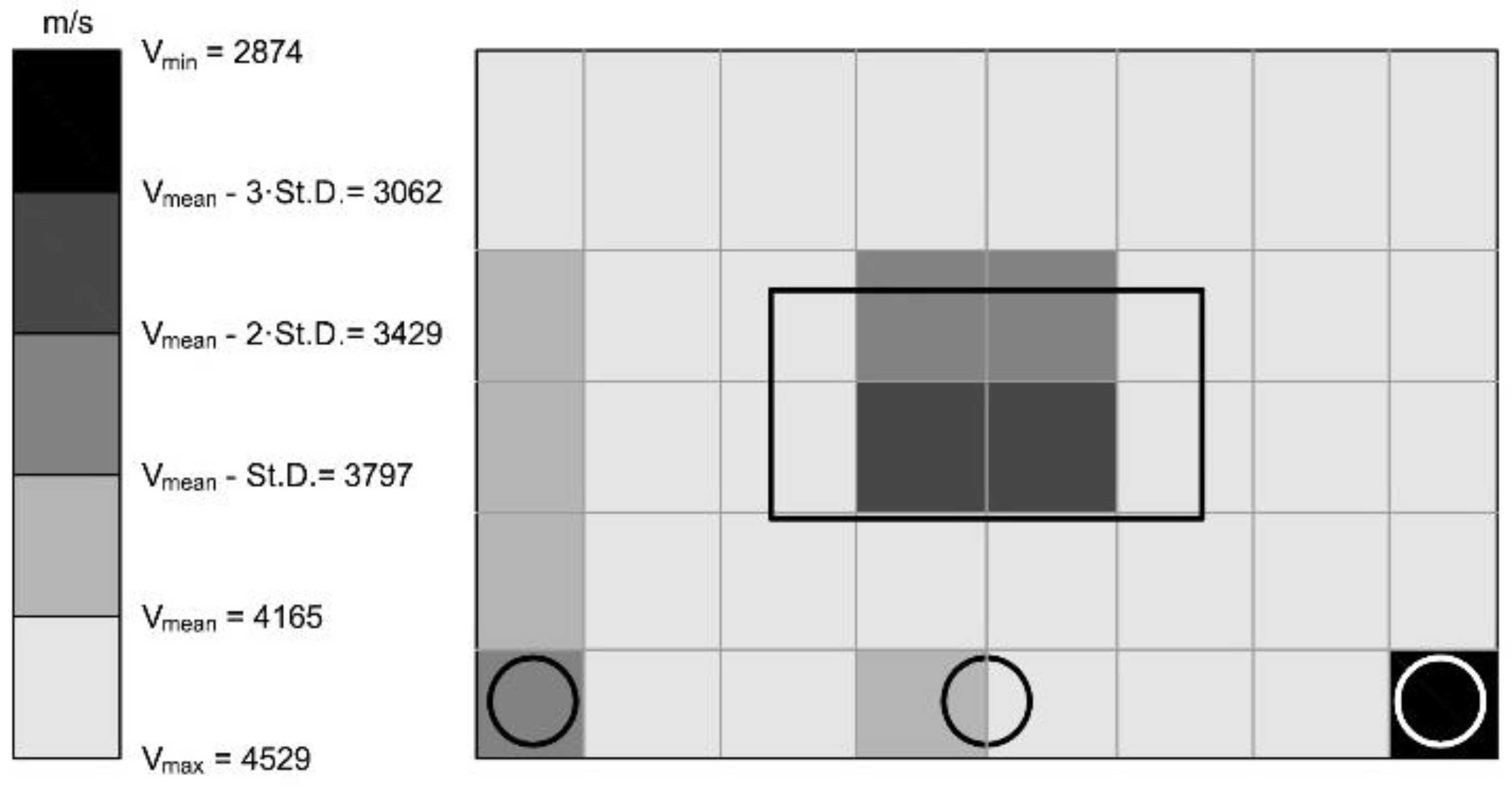
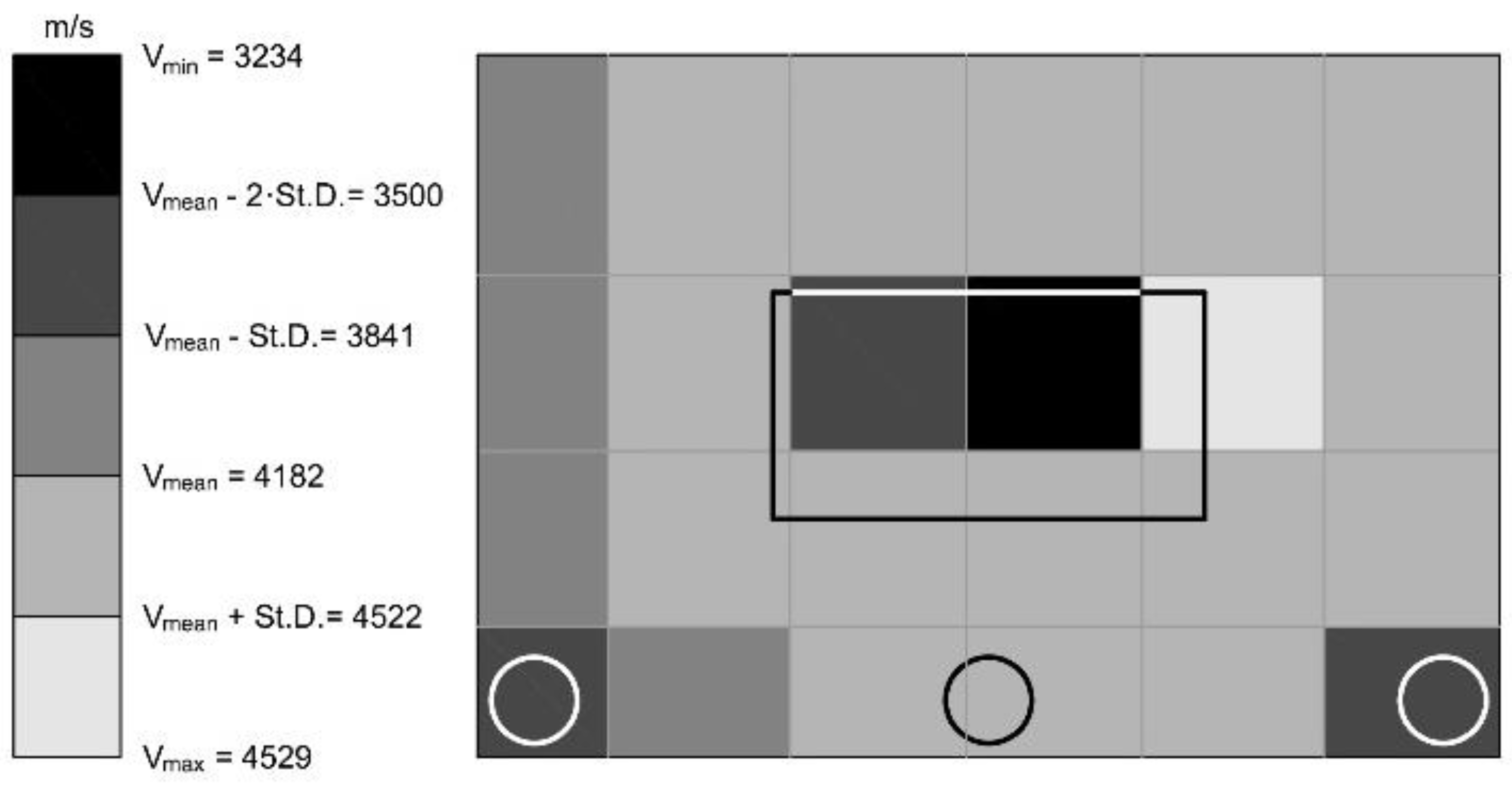
4.1.1. Velocity Maps. Type 1

In the first type of velocity maps, the range Vmax–Vmin has been divided into levels defined by:
V m e a n ± ( i ) S t . D . ,
where i is an integer ranging from 1 to a number depending on Vmax–Vmin. The outer levels, bordered by Vmax and Vmin respectively, are generally smaller than St.D. The values of V have, therefore, been grouped within the defined levels. Figure 3, Figure 4, Figure 5, Figure 6 and Figure 7 show the resulting maps (named 1 to 5) for measurements grids A to E, respectively, along with the actual position and size of the defects.
As shown in Figure 3, Figure 4, Figure 5, Figure 6 and Figure 7, the maps provide an immediate visualization of the presence and position of factors that determine anomalies in the propagation of the signals and, therefore, in V values.
By comparing the areas highlighted in the maps with the actual position and size of the defects, it can be notice the influence of both the pitch of the measurement grid and the position of the transducers with respect to the defect (transducers are assumed to act in the central point of the cells). Grid A (map 1, Figure 3), which is the densest having an average cells size of 0.04 m in both horizontal and vertical directions, provides the largest amount of information concerning the inside of the wall despite the lowest scattering of V data (see Table 2), which generally would be indicative of a homogeneous material. A detailed interpretation of all the information is not an easy task, because signal propagation is affected not only by the presence of the defects but also by all the changes of the inner structure of the wall, such as the variation of the consistency of concrete due to not perfect casting or the presence of gap-graded aggregates, and of the characteristics of the external surfaces, such as texture and roughness. Nevertheless, all the defects are detected with good accuracy, as testified by the number and the position of darker cells. It is worth noting the presence of a kind of boundary effect which causes V measured in correspondence of the edges to be generally slightly lower than V measured in the areas without known defects. This might depend on the disturbance due to reflection, refraction and scattering phenomena occurring at the edges of the wall. As soon as the grid thins out, the amount of information concerning the inside of the wall decreases, as well as the boundary effect, whereas the chance of differentiate between defective areas and boundary effect decreases. The artificial defects are still visible, although with less accuracy. In particular, in maps 3 and 4 (Figure 5 and Figure 6) the plastic disc P2 is not yet detectable and the empty box MC is more underestimated; these facts are also due to the eccentricity between the defects and the measurement points (the center of the cells).
This type of maps allows to collect information on the inside of the wall and to identify the presence of areas characterized by anomalous V distribution, thus giving a valuable picture of the wall. Nevertheless, an accurate sizing of the artificial defects is difficult, as well as the selection of the more suitable grid, because of the already mentioned effect on V of the inner characteristics and the geometry of the wall.

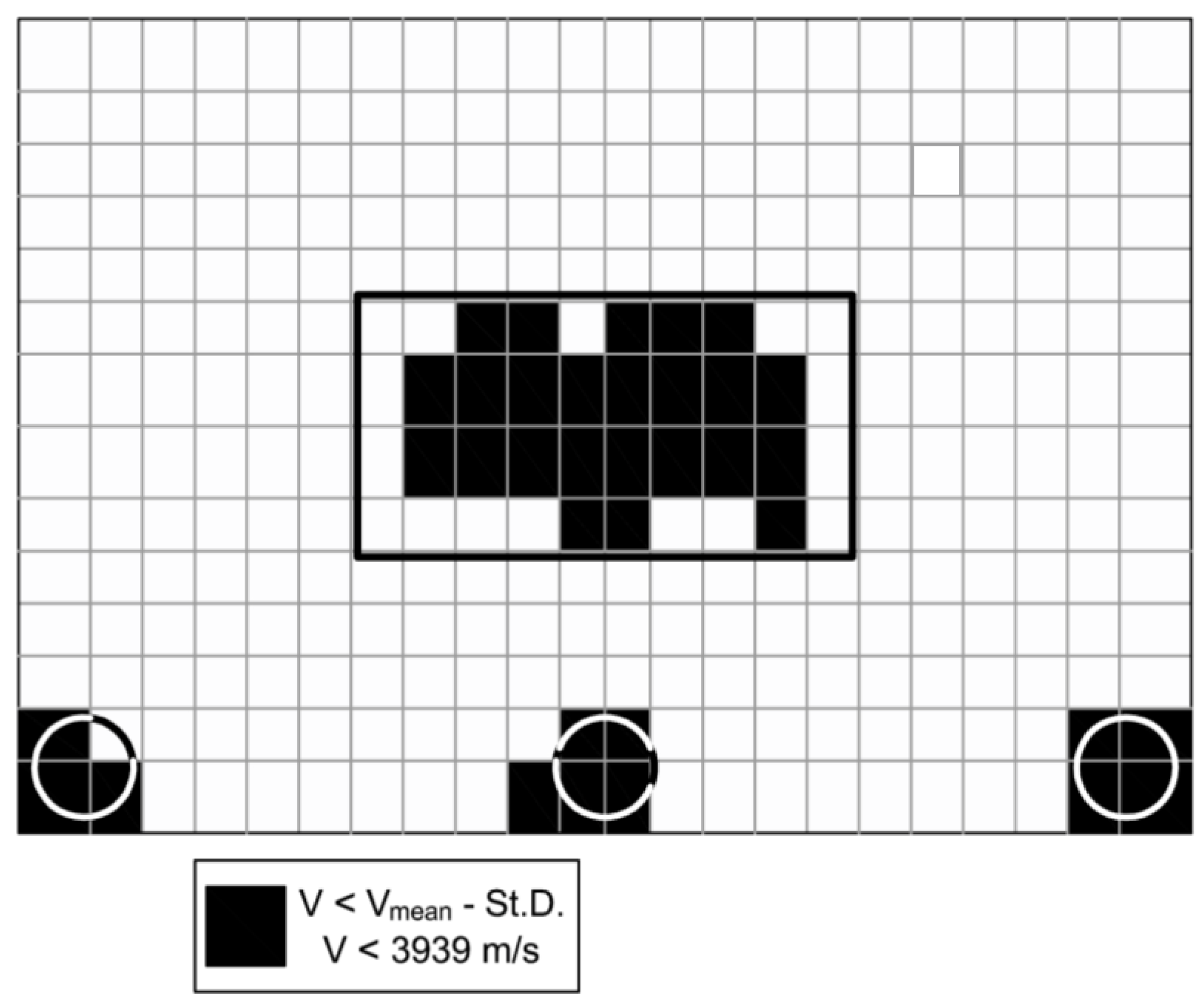
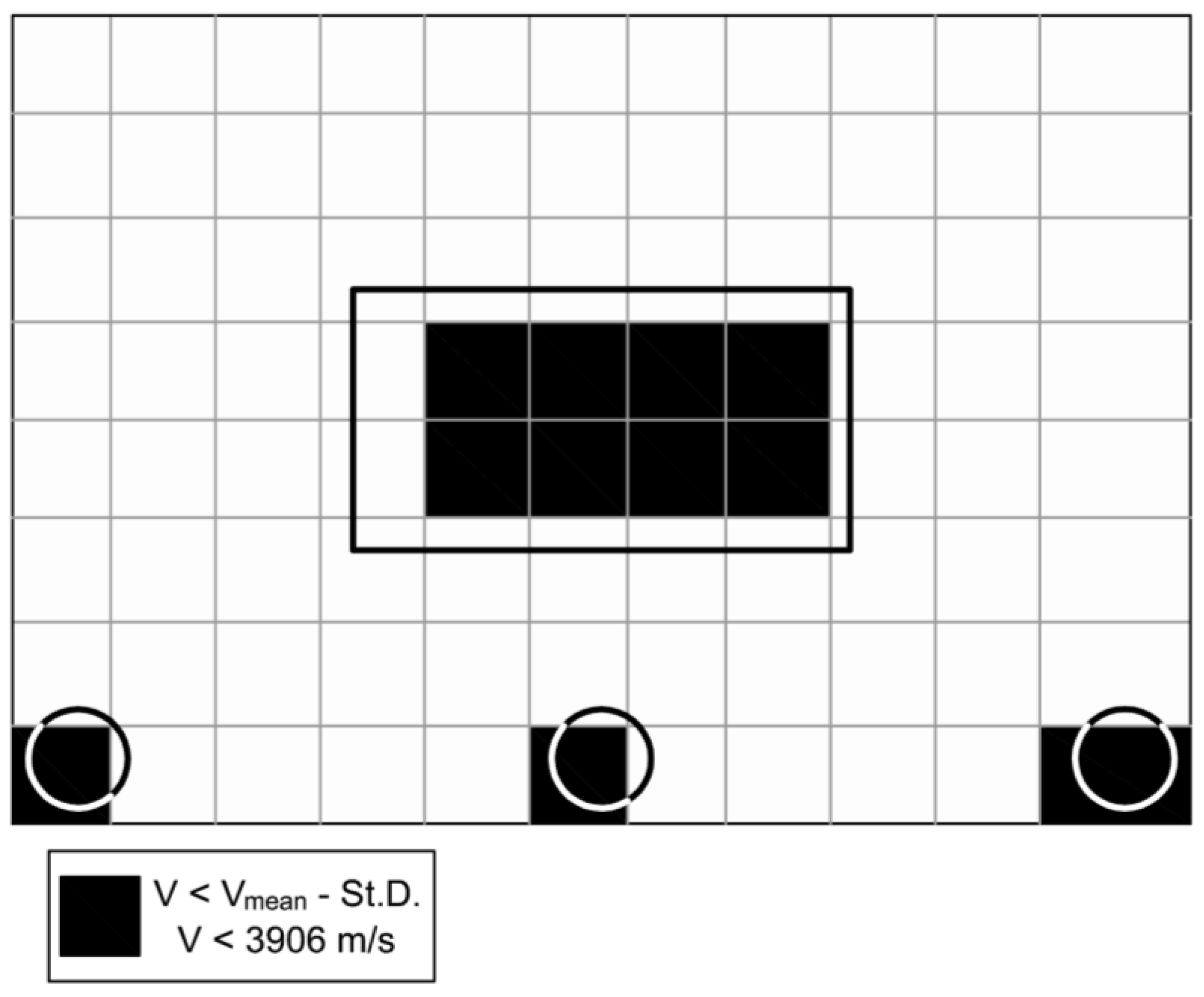
4.1.2. Velocity Maps. Type 2

In order to facilitate the location and sizing of the defects, even if at the price of losing some information, a second type of velocity maps has been implemented. V data have been considered anomalous only when:
V < V m e a n S t . D . ,
Figure 8, Figure 9, Figure 10, Figure 11 and Figure 12 show the resulting maps (named 6 to 10) for grids A to E, respectively.
As shown in Figure 8, Figure 9, Figure 10, Figure 11 and Figure 12, these maps highlight only areas corresponding to the defects. The maps point out all defects except P2, that again is not yet detectable by grids D and E (Figure 9 and Figure 11) because of the eccentricity between the defect and the measurement point.
These maps can be used for defect sizing, as discussed in the following section.

5. Defect Sizing

In order to evaluate the accuracy of maps 6–10 in sizing the artificial defects, for each defect an index I has been calculated as follows:
I = ( A e s t A a c t ) 100 100 ,
where Aest is the sum of the areas of the dark cells highlighted by the map and Aact is the actual area of the defect. The values of I are summarized in Table 3, while Figure 13 shows a comparison between the accuracy of the measurement grids. The empty box MC is detected by all grids and is always underestimated. The best accuracy (Figure 13) is provided by grid D (average cell size = 0.12 m), which corresponds to map 9 (Figure 11). The plastic disc P1 is detected by all grids. The best accuracy (Figure 13) is provided by grid C (average cell size = 0.08 m), which corresponds to map 8 (Figure 10). The plastic disc P2 is detected only by grids A, B, and C. The best accuracy (Figure 13) is provided by grid A (average cell size = 0.04 m), which corresponds to map 6 (Figure 8). The plastic disc P3 is detected by all grids. The best accuracy (Figure 13) is provided by grid B (average cell size = 0.08 m × 0.04 m), which corresponds to map 7 (Figure 9).
Figure 14 shows better the variability of the I index within the type of defect.
As previously noted, the identification and sizing of the empty box MC is less affected than the other defects by the spacing of the measurement grid, which, on the contrary, affects substantially the detection and sizing of the plastic discs P1, P2, and P3. This aspect mainly depends on the relationship between the mesh of the grid and the size of the defect. It is worth noting that maps 9 and 10 (Figure 11 and Figure 12), which correspond to measurement grids having average cells size greater than the diameter of the plastics discs, provide the lower accuracy for these defects. In detail, defects P1 and P3 are largely overestimated, while defect P2 is not detected because of an unfavorable combination of cells size and eccentricity between the cells center (measurement points) and the defect itself. The relationship between the accuracy and the pitch of the grid is illustrated in Figure 15 with reference to the grid spacing in the horizontal direction X. The trend lines related to the plastic defects clearly show the increase of the error as the size of the grid increases with respect to the size of the defect. This behavior arises starting from values of the grid pitch equal to the size of the defect.

6. Comments

The tests performed on the concrete wall have pointed out that the choice of the measurement grid significantly influences the diagnostic capacity of UT. The most significant parameter to take into consideration is the proportion between the grid pitch and the size of the defect. As shown in Figure 15, as the grid spacing exceeds the size of the defect, the error made by UT in estimating the size of the defect increases significantly. On the other hand, the capacity of sizing defects sufficiently greater than the grid cells, such as the empty box MC, is less affected by grid spacing variation, although the defect is underestimated by all the grids. The other factor that influences the accuracy of the method is the misalignment between the center of the grid cell, which corresponds to the point of input of the signal in the material, and the position of the defect. This factor can cause considerable errors in the estimate of the size of the defect, especially when it occurs concurrently with the use of grids with a pitch greater than the size of the defect (Figure 11 and Figure 12).
In order to further highlight the importance of the topic, an analogy can be made between the laboratory case analyzed and real cases of defects in concrete. When considering anomalies in concrete elements and structures, it should be taken into account that the causes of defects differ according to the period in which they arise. They can arise: before construction, such as design errors; during the construction phases, such as errors of execution and realization; during the normal use of the building, such as overloading and environmental effects; as a consequence of exceptional events as earthquake, fire, impacts; as a result of anthropic actions, such as extension works and changing in end use [54]. Some of these causes give rise to phenomena known as segregation of concrete, cracking, spalling and delamination, that result in the formation on the surface of the element or within its volume of more or less important voids and discontinuities, often referred to as rock pockets, honeycombs, cracks, delamination, and detachment. The presence of such internal defects can impact overall stiffness, accelerate aging, reduce service life and cause structural problems, being the severity of the degradation of the concrete element proportional to the size of the defect [55,56,57].
Let us consider a reinforced concrete element, for example a vertical one such as a pillar or a wall, in which a segregation phenomenon occurred during hardening, determining the formation of a volume full of cavities that can be assimilated by size to the MC of the test. This kind of defect is commonly simulated by means of embedded voids [58,59,60,61,62] as the MC of the test. Figure 16 shows the overestimate of the usable cross section of the element net of the section of the defect as a function of the size of the defect and of the I index reported in Table 3.
The figure shows the effect of underestimating the size of the defect on the value of the area of the resistant section, which can be overestimated even by 40% with serious detriment of the static safety. As an example and by accepting a rough calculation, if the element is loaded by axial compression the overlap of the resistant section results in a corresponding overestimate of the section capacity load. Similarly, if we consider the presence of a delamination or detachment area that can be assimilated to the plastic elements P1,2,3 of the test, as is common in literature [61,62,63,64], depending on the spacing and the position of the measurement points the defect is not detected or it is overestimated even by 150%. Additionally, in this case there can be repercussions on the correct evaluation of the structural integrity and therefore on the refurbishment planning.
In the light of these considerations, the complexity of defining an optimal grid to make the most of the UT capabilities to identify and size the defects present inside the concrete element clearly emerges. The criterion for choosing the grid mesh should be based on a prior idea of the type and size of the defects to be detected. From this perspective, it is necessary to keep in mind some aspects:
  • small defects are more difficult to identify but are also generally less important from an engineering point of view;
  • more refined measurements grids are more sensitive to the presence of defects, but at the same time they are strongly affected by the intrinsic irregularity of the material, which influences the propagation of the signal and, thus, its velocity;
  • when the goal is a qualitative preliminary diagnosis of the concrete element or structure, less refined grids are already sufficient and facilitate both the execution of the tests and the data analysis; and
  • the timing and costs of the tests cannot be ignored.
Starting from the results of the present experimentation, a possible operative methodology is the following: UT data can be first implemented accordingly to velocity maps of type 1, in order to gather comprehensive information regarding the inside of the concrete element, choosing the grid pitch according to the geometry of the problem and the expected results and eventually repeating the tests with different grid spacing; after that, once the areas potentially affected by defects of interest have been established, the data can be implemented according to velocity maps of type 2, aiming to locate and size the defects. In this second phase the choice of the grid should be made according to the minimum size of the defect to be determined.

7. Conclusions

This paper illustrates the results of an experimental test aimed to check the efficacy of ultrasonic testing (UT) in detecting anomalies inside concrete elements by taking into account the influence of the measurements grid arrangement.
UT has been carried out on a small concrete wall in which some defects have been settled during casting: an empty box of polystyrene assumed as a macro-cavity (MC), and three plastic discs (P1, P2, P3) assumed as small sub-surface defects. UT measurements have been performed by applying the direct transmission technique (DTT). Five measurements grids, having different spacing, have been realized by marking the emitting and receiving points on the opposite surfaces of the wall. For each point the ultrasonic signal has been transmitted and acquired, and the velocity of propagation V has been extracted and analyzed. Then, for each grid the distribution of V data has been graphically represented by implementing two different types of velocity maps where each cell identifies one emitter-receiver couple—and one value of V—and is representative of its neighborhood.
The following conclusions can be drawn.
  • The five measurements grids show similar value of Vmax and Vmean and a slight difference in Vmin, which is the most scattered property accordingly to the fact that defects slow down the velocity of the signals that are diffracted around the periphery of the defect, whereas highest values of V are generally reached in points without defects regardless of the presence or not of some defects in other areas of the wall. This finding confirms the sensitivity of V to the presence of anomalies inside the concrete.
  • The velocity maps of type 1, based on the definition of various V levels, allow to collect information on the inside of the wall and to identify the presence of areas characterized by anomalous V distribution, thus, giving a valuable picture of the wall. Nevertheless, an accurate sizing of the artificial defects is difficult because signals propagation is affected not only by the artificial defects but also by all changes of the inner structure of the wall.
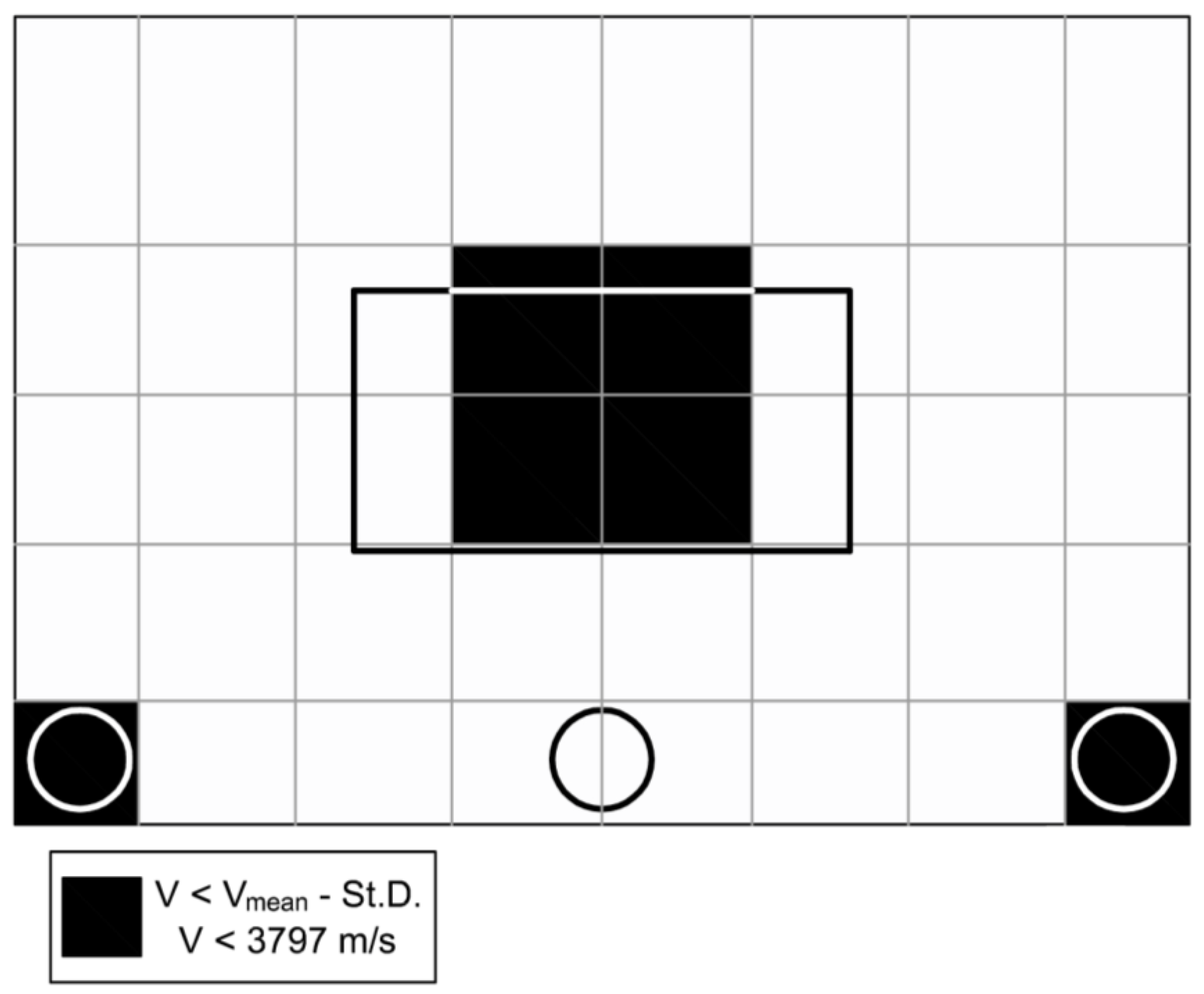
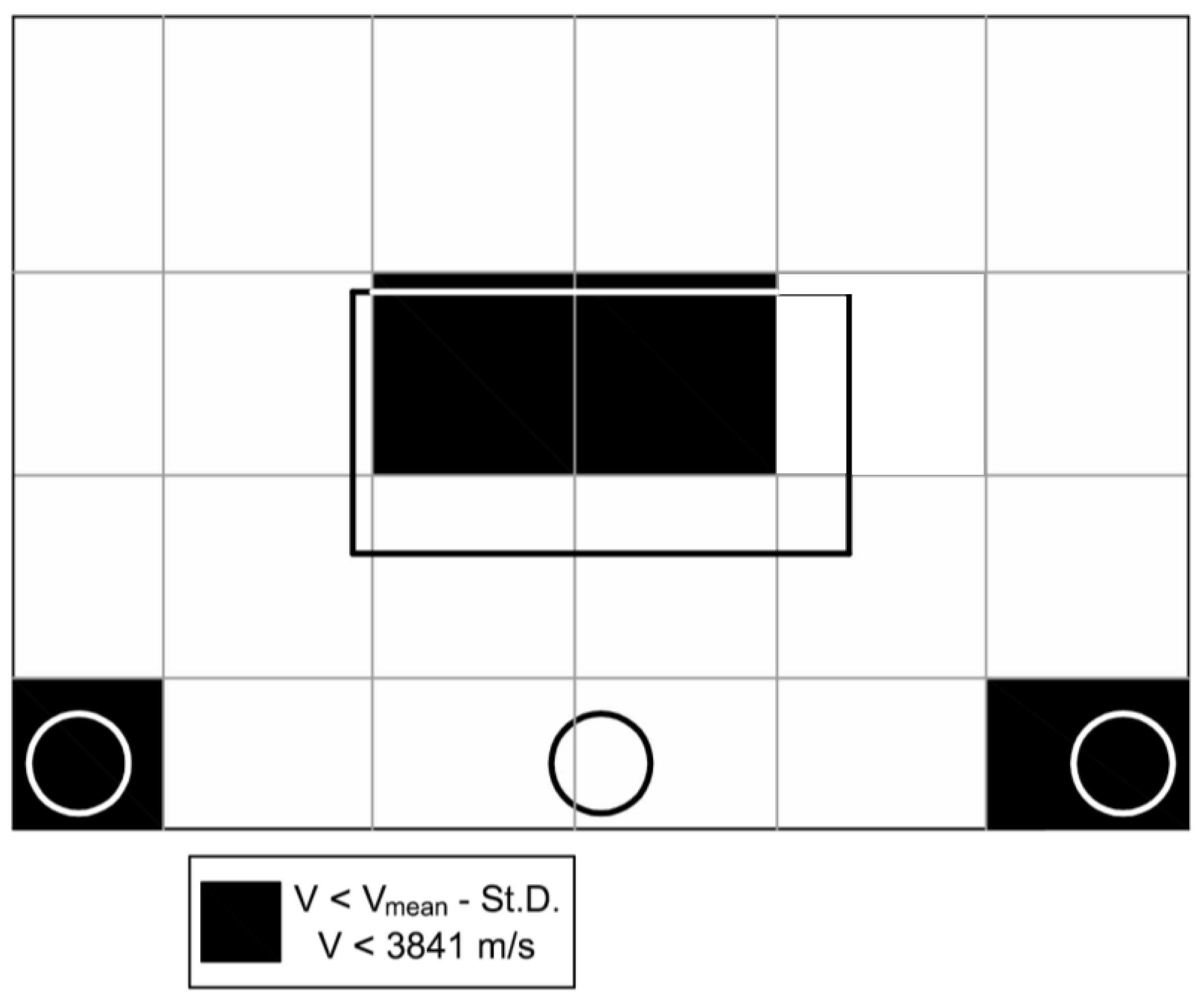
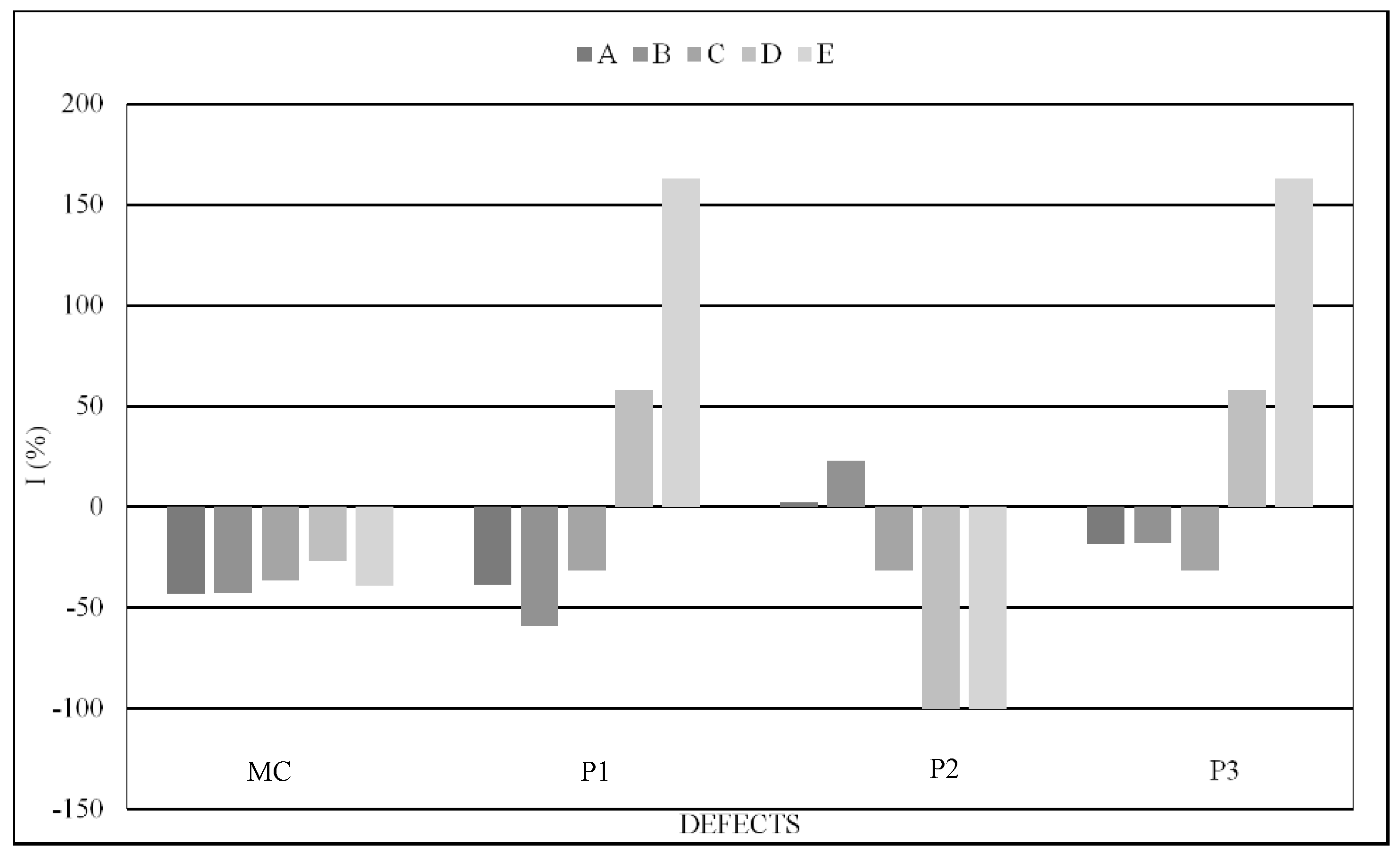
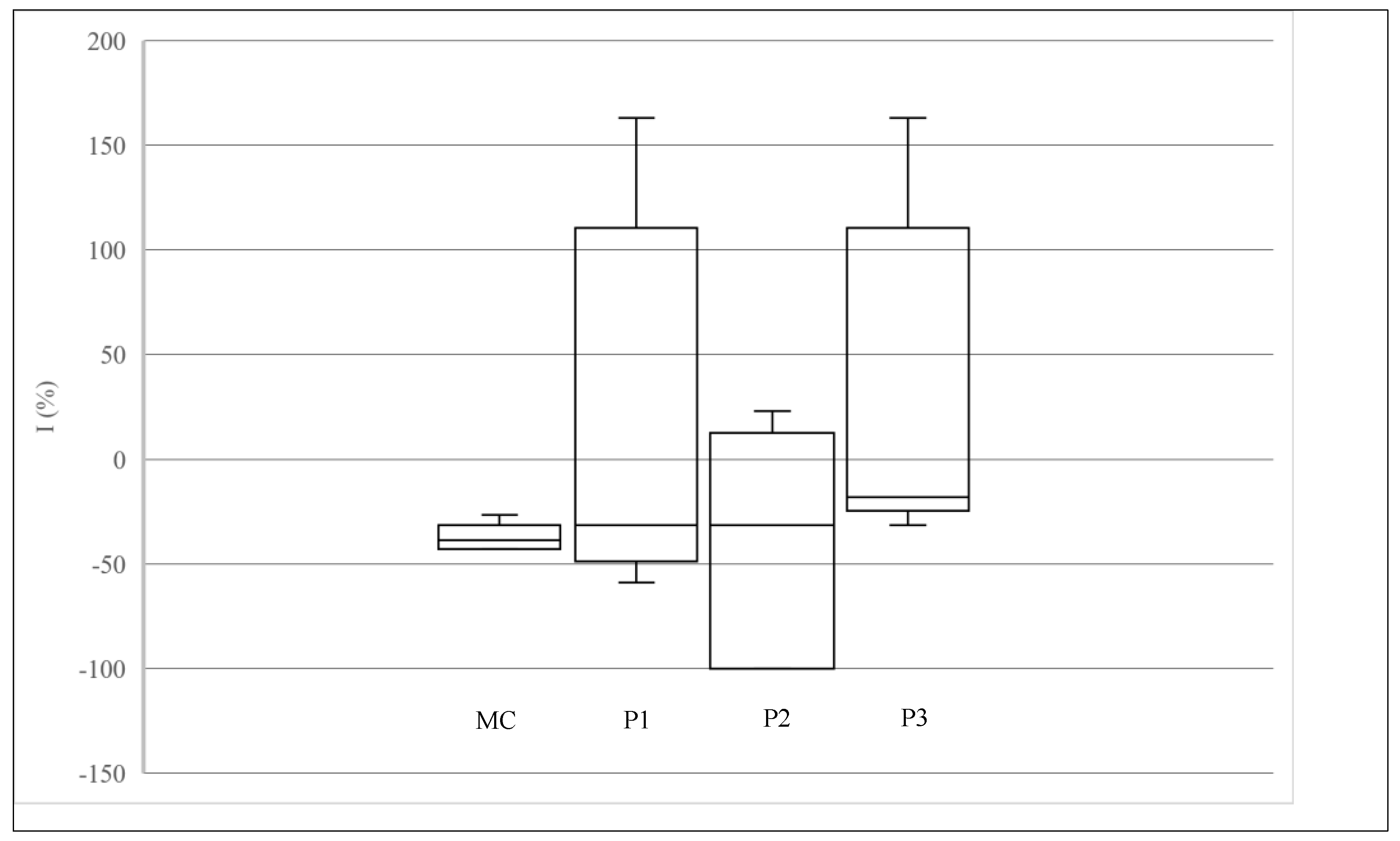
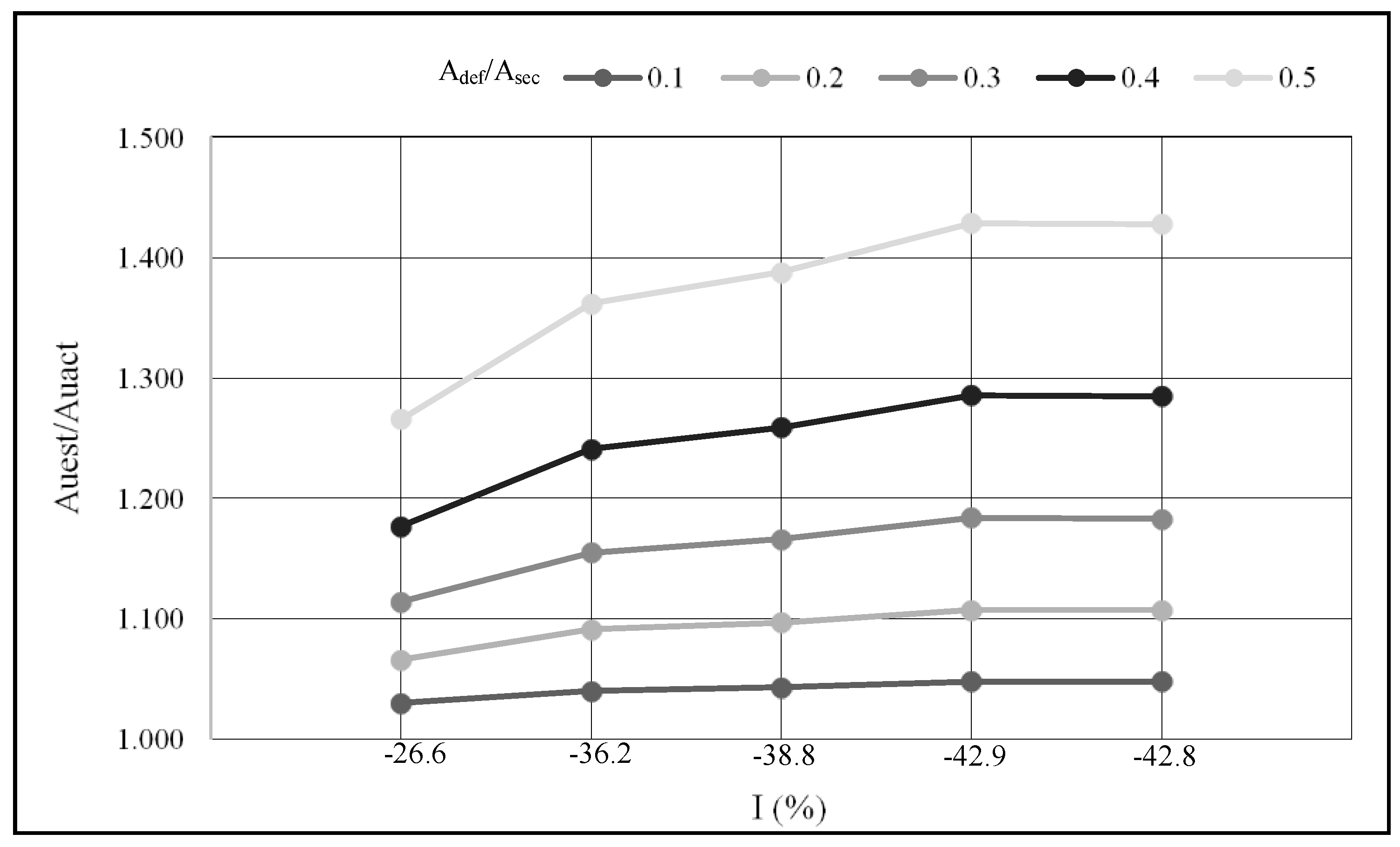
  • The velocity maps of type 2 have been implemented in order to highlight only the artificial defects, even if at the price of losing some information, and have been used to define a criterion for evaluating the accuracy of V maps in sizing the artificial defects based on an index I that takes into account the sum Aest of the area of dark cells highlighted by the map and the actual area of the defect Aact.
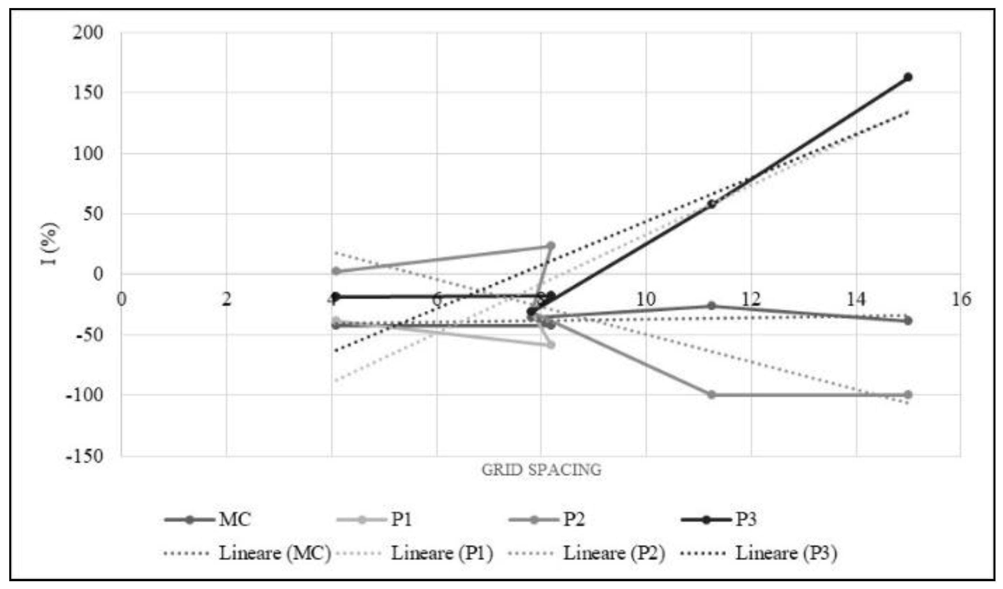
  • The choice of the measurements grid significantly influences the diagnostic capacity of UT. The proportion between the grid pitch and the size of the defect, along with the misalignment between the center of the grid cell and the position of the defect, are the most influencing factors. It has been pointed out that as the grid spacing exceeds the size of the defect, the error made by UT in estimating the size of the defect increases significantly and that the unfavorable combination of cells size and eccentricity between the cells center and the defect itself could lead to very large miscalculating in defect sizing.
The results since now achieved suggest that velocity maps are powerful tools for concrete defects identification. In order to optimize the diagnostic capabilities of the method, finding a compromise between maximum accuracy and minimum test times, UT data should be first implemented accordingly to velocity maps of type 1, in order to gather comprehensive information regarding the inside of the concrete element, and then accordingly to the velocity maps of type 2, aiming to locate and size the inner defects. The importance of measurement points spacing and position, which clearly emerges from the present experimentation and which has not been analyzed sufficiently and comprehensively in the existing literature, suggests the need of deepening this topic and encourages the future implementation of design criteria for the measurement grids in standards and guidelines related to UT. In conclusion, the presented study allows us to shed light on an aspect of UT since now not sufficiently addressed in the literature, and provides important and useful results to understand the importance of the problem and to suggest the opportunity for further research, for example by varying the type and characteristics of the concrete defects.

Author Contributions

Conceptualization: G.C.; data curation: G.C. and N.T.; funding acquisition: G.C.; investigation: G.C. and N.T.; methodology: G.C. and N.T.; supervision: G.C.; writing—original draft: G.C.; writing—review and editing: G.C.

Funding

This research was supported by the research grant for the project “Healthy Cities and Smart Territories” (2016/17) funded by Fondazione di Sardegna and the Autonomous Region of Sardinia.

Conflicts of Interest

The authors declare no conflict of interest. The funders had no role in the design of the study; in the collection, analyses, or interpretation of data; in the writing of the manuscript; or in the decision to publish the results.

References

  1. Boosting Building Renovation: What Potential and Value for Europe? Directorate General for Internal Policies Policy Department A: Economic and Scientific Policy. Available online: http://www.europarl.europa.eu/RegData/etudes/STUD/2016/587326/IPOL_STU(2016)587326_EN.pdf (accessed on 19 November 2018).
  2. CRESME Technical Report. 2017. Available online: http://www.cresme.it/doc/rapporti/rapporto-cresme-symbola-2017.pdf (accessed on 19 november 2018).
  3. Frangopol, D.M.; Liu, M. Maintenance and management of civil infrastructure based on condition, safety, optimization, and life-cycle cost. Struct. Infrastruct. Eng. 2007, 3, 29–41. [Google Scholar] [CrossRef]
  4. Frangopol, D.M.; Saydam, D.; Kim, S. Maintenance, management, life-cycle design and performance of structures and infrastructures: A brief review. Struct. Infrastruct. Eng. 2012, 8, 1–25. [Google Scholar] [CrossRef]
  5. Jensen, P.A.; Maslesa, E. Value based building renovation—A tool for decision making. Build. Environ. 2015, 92, 1–9. [Google Scholar] [CrossRef] [Green Version]
  6. Fib Bulletin N° 22. Monitoring and Safety Evaluation of Existing Concrete Structures; State-of-Art Report; fib: Lausanne, Switzerland, May 2003. [Google Scholar]
  7. Fib Bulletin N° 17. Management, Maintenance and Strengthening of Concrete Structures; Technical Report; fib: Lausanne, Switzerland, April 2002. [Google Scholar]
  8. McCann, D.M.; Forde, M.C. Review of NDT methods in the assessment of concrete and masonry structures. Ndt E Int. 2001, 34, 71–84. [Google Scholar] [CrossRef]
  9. Hussain, A.; Akhtar, S. Review of non-destructive tests for evaluation of historic masonry and concrete structures. Arab. J. Sci. Eng. 2017, 42, 925–940. [Google Scholar] [CrossRef]
  10. Moropoulou, A.; Labropoulos, K.C.; Delegou, E.T.; Karoglou, M.; Bakolas, A. Non-destructive techniques as a tool for the protection of built cultural heritage. Constr. Build. Mater. 2013, 48, 1222–1239. [Google Scholar] [CrossRef]
  11. Concu, G.; Nicolo, B.D.; Pani, L. Non-destructive testing as a tool in reinforced concrete buildings refurbishments. Struct. Surv. 2011, 29, 147–161. [Google Scholar] [CrossRef]
  12. Rehman, S.K.U.; Ibrahim, Z.; Memon, S.A.; Jameel, M. Nondestructive test methods for concrete bridges: A review. Constr. Build. Mater. 2016, 107, 58–86. [Google Scholar] [CrossRef] [Green Version]
  13. Blitz, J. Electrical and Magnetic Methods of Non-Destructive Testing, 2nd ed.; Springer Science & Business Media: Dordrecht, The Netherlands, 1997; ISBN 9789401158183. [Google Scholar]
  14. Maierhofer, C.; Reinhardt, H.W.; Dobmann, G. Non-Destructive Evaluation of Reinforced Concrete Structures: Non-Destructive Testing Methods; Woodhead Publishing: Cambridge, UK, 2010; ISBN 9781845699604. [Google Scholar]
  15. Popovics, J.S. Ultrasonic testing of concrete structures. Mater. Eval. 2005, 63, 50–55. [Google Scholar]
  16. De Nicolo, B.; Piga, C.; Popescu, V.; Concu, G. Non-Invasive Acoustic Measurements for Faults Detecting in Building Materials and Structures. In Applied Measurement Systems; Haq, Z., Ed.; InTech: Rijeka, Croatia, 2012; ISBN 978-953-51-0103-1. [Google Scholar]
  17. Krause, M.; Mielentz, F.; Milman, B.; Müller, W.; Schmitz, V.; Wiggenhauser, H. Ultrasonic imaging of concrete members using an array system. Ndt E Int. 2001, 34, 403–408. [Google Scholar] [CrossRef]
  18. Schickert, M.; Krause, M.; Müller, W. Ultrasonic imaging of concrete elements using reconstruction by synthetic aperture focusing technique. J. Mater. Civ. Eng. 2003, 15, 235–246. [Google Scholar] [CrossRef]
  19. De Nicolo, B.; Mistretta, F.; Concu, G. NDT ultrasonic evaluation of early compressive strength in SCC. In Proceedings of the 9th International Conference on Inspection, Appraisal, Repairs and Maintenance of Structures, Fuzhou, China, 20–21 October 2005; pp. 187–194, ISBN 981-05-3548-1. [Google Scholar]
  20. Del Río, L.M.; Jiménez, A.; López, F.; Rosa, F.J.; Rufo, M.M.; Paniagua, J.M. Characterization and hardening of concrete with ultrasonic testing. Ultrasonics 2004, 42, 527–530. [Google Scholar] [CrossRef] [PubMed]
  21. Trtnik, G.; Gams, M. Ultrasonic assessment of initial compressive strength gain of cement based materials. Cem. Concr. Res. 2015, 67, 148–155. [Google Scholar] [CrossRef]
  22. Trtnik, G.; Gams, M. Recent advances of ultrasonic testing of cement based materials at early ages. Ultrasonics 2014, 54, 66–75. [Google Scholar] [CrossRef] [PubMed]
  23. Concu, G.; De Nicolo, B.; Mistretta, F.; Pani, L. Ultrasonic test methods for assessment of concrete strength during construction. In Proceedings of the 10th International Conference on Inspection, Appraisal, Repairs and Maintenance of Structures, Hong Kong, China, 25–26 October 2006; pp. 83–88, ISBN 981-05-5562-8. [Google Scholar]
  24. Popovics, J.S.; Subramaniam, K.V. Review of ultrasonic wave reflection applied to early-age concrete and cementitious materials. J. Nondestruct. Eval. 2015, 34, 267. [Google Scholar] [CrossRef]
  25. Haach, V.G.; Juliani, L.M.; Roz, M.R.D. Ultrasonic evaluation of mechanical properties of concretes produced with high early strength cement. Constr. Build. Mater. 2015, 96, 1–10. [Google Scholar] [CrossRef]
  26. Zhao, Y.; Hao, W.; Xu, X. Experimental study of the working stress state of concrete frame structures through ultrasonic testing. Chem. Eng. Trans. 2017, 62, 919–924. [Google Scholar]
  27. Ivanchev, I. Experimental determination of concrete compressive strength by non-destructive ultrasonic pulse velocity method. Int. J. Res. Appl. Sci. Eng. Technol. 2018, 6. [Google Scholar] [CrossRef]
  28. Nogueira, C.L.; Willam, K.J. Ultrasonic testing of damage in concrete under uniaxial compression. Mater. J. 2001, 98, 265–275. [Google Scholar]
  29. Abo-Qudais, S.A. Effect of concrete mixing parameters on propagation of ultrasonic waves. Constr. Build. Mater. 2005, 19, 257–263. [Google Scholar] [CrossRef]
  30. Kewalramani, M.A.; Gupta, R. Concrete compressive strength prediction using ultrasonic pulse velocity through artificial neural networks. Autom. Constr. 2006, 15, 374–379. [Google Scholar] [CrossRef]
  31. Concu, G.; De Nicolo, B.; Trulli, N.; Valdes, M. Estimation of concrete strength and stiffness by means of ultrasonic testing. In Concrete Repair, Rehabilitation and Retrofitting IV; Dehn, F., Beushausen, H.-D., Alexander, M.G., Moyo, P., Eds.; Taylor & Francis Group: London, UK, 2016; ISBN 978-113802843-2. [Google Scholar]
  32. Hernández, M.G.; Izquierdo, M.A.G.; Ibáñez, A.; Anaya, J.J.; Ullate, L.G. Porosity estimation of concrete by ultrasonic NDE. Ultrasonics 2000, 38, 531–533. [Google Scholar] [CrossRef]
  33. Benmeddour, F.; Villain, G.; Abraham, O.; Choinska, M. Development of an ultrasonic experimental device to characterise concrete for structural repair. Constr. Build. Mater. 2012, 37, 934–942. [Google Scholar] [CrossRef]
  34. Moradi, F.; Rivard, P.; Lamarche, C.P.; Kodjo, S.A. Evaluating the damage in reinforced concrete slabs under bending test with the energy of ultrasonic waves. Constr. Build. Mater. 2014, 73, 663–673. [Google Scholar] [CrossRef]
  35. Molero, M.; Aparicio, S.; Al-Assadi, G.; Casati, M.J.; Hernández, M.G.; Anaya, J.J. Evaluation of freeze–thaw damage in concrete by ultrasonic imaging. Ndt E Int. 2012, 52, 86–94. [Google Scholar] [CrossRef] [Green Version]
  36. Toutanji, H. Ultrasonic wave velocity signal interpretation of simulated concrete bridge decks. Mater. Struct. 2000, 33, 207–215. [Google Scholar] [CrossRef]
  37. Shah, A.A.; Ribakov, Y. Non-linear ultrasonic evaluation of damaged concrete based on higher order harmonic generation. Mater. Des. 2009, 30, 4095–4102. [Google Scholar] [CrossRef]
  38. Antonaci, P.; Bruno, C.L.E.; Gliozzi, A.S.; Scalerandi, M. Monitoring evolution of compressive damage in concrete with linear and nonlinear ultrasonic methods. Cem. Concr. Res. 2010, 40, 1106–1113. [Google Scholar] [CrossRef]
  39. Antonaci, P.; Bruno, C.L.E.; Bocca, P.G.; Scalerandi, M.; Gliozzi, A.S. Nonlinear ultrasonic evaluation of load effects on discontinuities in concrete. Cem. Concr. Res. 2010, 40, 340–346. [Google Scholar] [CrossRef]
  40. Rucka, M.; Wilde, K. Experimental study on ultrasonic monitoring of splitting failure in reinforced concrete. J. Nondestruct. Eval. 2013, 32, 372–383. [Google Scholar] [CrossRef]
  41. Adamatti, D.S.; Lorenzi, A.; Chies, J.A.; Silva Filho, L.C.P. Analysis of reinforced concrete structures through the ultrasonic pulse velocity: Technological parameters involved. Rev. IBRACON Estrut. Mater. 2017, 10, 358–385. [Google Scholar] [CrossRef]
  42. Concu, G.; De Nicolo, B.; Trulli, N.; Valdes, M. Transducers frequency influence on ultrasonic velocity measurements in concrete specimens. In Research and Applications in Structural Engineering, Mechanics and Computation; Taylor & Francis Group: London, UK, 2013; ISBN 9781138000612. [Google Scholar]
  43. Lorenzi, A.; Caetano, L.F.; Chies, J.A.; Pinto da Silva Filho, L.C. Investigation of the potential for evaluation of concrete flaws using nondestructive testing methods. ISRN Civ. Eng. 2014, 2014, 543090. [Google Scholar] [CrossRef]
  44. EN 12504-4. Testing Concrete—Part 4: Determination of Ultrasonic Pulse Velocity; British Standards Institution: London, UK, 2004. [Google Scholar]
  45. Guidelines for the Evaluation of Concrete Characteristics On-Site. High Council for Public Works—Central Technical, Service, 2017. Available online: http://cslp.mit.gov.it/index.php?option=com_content&task=view&id=157&Itemid=20 (accessed on 19 November 2018).
  46. Krautkramer, J.; Krautkramer, H. Ultrasonic Testing of Materials; Springer-Verlag Berlin Heidelberg GmbH: Berlin/Heidelberg, Germany, 1990. [Google Scholar]
  47. Berke, M. Non-destructive material testing with ultrasonics. Introduction to the basic principles. NDT.net 2000, 5, 9. [Google Scholar]
  48. Mahure, N.V.; Vijh, G.K.; Sharma, P.; Sivakumar, N.; Ratnam, M. Correlation between pulse velocity and compressive strength of concrete. Int. J. Earth Sci. Eng. 2011, 4, 871–874. [Google Scholar]
  49. Bogas, J.A.; Gomes, M.G.; Gomes, A. Compressive strength evaluation of structural lightweight concrete by non-destructive ultrasonic pulse velocity method. Ultrasonics 2013, 53, 962–972. [Google Scholar] [CrossRef]
  50. Demirboga, R.; Türkmen, İ.; Karakoç, M.B. Relationship between ultrasonic velocity and compressive strength for high-volume mineral-admixtured concrete. Cem. Concr. Res. 2004, 34, 2329–2336. [Google Scholar] [CrossRef]
  51. Lafhaj, Z.; Goueygou, M.; Djerbi, A.; Kaczmarek, M. Correlation between porosity, permeability and ultrasonic parameters of mortar with variable water/cement ratio and water content. Cem. Concr. Res. 2006, 36, 625–633. [Google Scholar] [CrossRef]
  52. Taffe, A.; Mayerhofer, C. Guidelines for NDT methods in civil engineering. In Proceedings of the 5th International Symposium on NDT in Civil Engineering, Berlin, Germany, 16–19 September 2003; German Society for Non-Destructive Testing: Berlin, Germany, 2003. ISBN 3-931381-49-8. [Google Scholar]
  53. Neville, A.M.; Brooks, J.J. Concrete Technology, 6th ed.; Longman Singapor Publishers Pte: Singapore, 1997. [Google Scholar]
  54. Macdonald, S. Concrete: Building Pathology; John Wiley & Sons: Hoboken, NJ, USA, 2008; ISBN 9781405147538. [Google Scholar]
  55. Sezer Atamturktur, H. Detection of Internal Defects in Concrete Members Using Global Vibration Characteristics. ACI Mater. J. 2013, 110, 1. [Google Scholar]
  56. Santos, J. Common pathologies in RC bridge structures: A statistical analysis. Electron. J. Struct. Eng. 2007, 7, 19–26. [Google Scholar]
  57. Garrido Vazquez, E.; Naked Haddad, A.; Linhares Qualharini, E.; Amaral Alves, L.; Amorim Féo, I. Pathologies in Reinforced Concrete Structures. In Sustainable Constructions Building Performance Simulation and Asset and Maintenance Management; Delgado, J.M.P.Q., Ed.; Springer: Singapore, 2016; ISBN 978-981-10-0650-0, 978-981-10-0651-7. [Google Scholar]
  58. Cheng, C.C.; Cheng, T.M.; Chiang, C.H. Defect detection of concrete structures using both infrared thermography and elastic waves. Autom. Constr. 2008, 18, 87–92. [Google Scholar] [CrossRef]
  59. Haach, V.G.; Ramirez, F.C. Qualitative assessment of concrete by ultrasound tomography. Constr. Build. Mater. 2016, 119, 61–70. [Google Scholar] [CrossRef]
  60. Maierhofer, C.; Brink, A.; Röllig, M.; Wiggenhauser, H. Detection of shallow voids in concrete structures with impulse thermography and radar. Ndt E Int. 2003, 36, 257–263. [Google Scholar] [CrossRef]
  61. Cotič, P.; Kolarič, D.; Bosiljkov, V.B.; Bosiljkov, V.; Jagličić, Z. Determination of the applicability and limits of void and delamination detection in concrete structures using infrared thermography. Ndt E Int. 2015, 74, 87–93. [Google Scholar] [CrossRef]
  62. Cotič, P.; Jagličić, Z.; Niederleithinger, E.; Stoppel, M.; Bosiljkov, V. Image fusion for improved detection of near-surface defects in ndt-ce using unsupervised clustering methods. J. Nondestruct. Eval. 2014, 33, 384–397. [Google Scholar] [CrossRef]
  63. Shin, S.W.; Oh, T.; Popovics, J.S. Identification of Delamination Damages in Concrete Structures Using Impact Response of Delaminated Concrete Section. In Proceedings of the 2013 World Congress on Advances in Structural Engineering and Mechanics, Jeiu, Korea, 8–12 September 2013; Techno-Press: Daejeon, Korea, 2013. [Google Scholar]
  64. Van der Wielen, A.; Courard, L.; Nguyen, F. Nondestructive Detection of Delaminations in Concrete Bridge Decks. In Proceedings of the XIII International Conference on Ground Penetrating Radar, Lecce, Italy, 21–25 June 2010; Institute of Electrical and Electronics Engineers (IEEE): Piscataway, NJ, USA, 2010. ISBN 9781424446049. [Google Scholar]
Figure 1. Vertical and horizontal sections of the concrete wall (dimensions are in meters).
Buildings 08 00176 g001
Figure 2. Transducer position in grid A (a) and scheme of transducers position in grid C (b).
Buildings 08 00176 g002
Figure 3. Map 1: Grid A. Levels of velocity.
Buildings 08 00176 g003
Figure 4. Map 2: Grid B. Levels of velocity.
Buildings 08 00176 g004
Figure 5. Map 3: Grid C. Levels of velocity.
Buildings 08 00176 g005
Figure 6. Map 4: Grid D. Levels of velocity.
Buildings 08 00176 g006
Figure 7. Map 5: Grid E. Levels of velocity.
Buildings 08 00176 g007
Figure 8. Map 6: Grid A. Defective areas.
Buildings 08 00176 g008
Figure 9. Map 7: Grid B. Defective areas.
Buildings 08 00176 g009
Figure 10. Map 8: Grid C. Defective areas.
Buildings 08 00176 g010
Figure 11. Map 9: Grid D. Defective areas.
Buildings 08 00176 g011
Figure 12. Map 10: Grid E. Defective areas.
Buildings 08 00176 g012
Figure 13. I index: comparison between the accuracy of measurement grids.
Buildings 08 00176 g013
Figure 14. Variability of the I index within the type of defect.
Buildings 08 00176 g014
Figure 15. Relationship between I index and grid spacing in X direction.
Buildings 08 00176 g015
Figure 16. Ratio between the estimated area of the usable cross section Auest and the actual area of the usable cross section Auact. Adef and Asec are the area of the cross section of the defect and of the element, respectively.
Buildings 08 00176 g016
Table 1. Grids information.
GridNumber of CellsX × 10−2 (m)Y × 10−2 (m)
A3084.084.43
B1548.184.43
C887.827.75
D4011.2512.40
E2415.0015.50
Table 2. Summary of UT measurements.
GridVmin (m/s)Vmax (m/s)Vmean (m/s)St.D. 1 (m/s)CoV 2 (%)
A287445404239299.797.07
B287445404240313.447.39
C309445294222315.757.48
D287445294165367.928.83
E323445294182340.898.15
Average299045334210--
St.D.166.376.0234.25--
1 St.D. = Standard Deviation, 2 CoV = Coefficient of Variation.
Table 3. I index.
Table 3. I index.
DefectGridAact × 10−4 [m2]Aest × 10−4 [m2]I [%]
MCA760.00433.79−42.9
B434.85−42.8
C484.84−36.2
D558.00−26.6
E465.00−38.8
P1A88.3654.22−38.6
B36.24−59.0
C60.61−31.4
D139.5057.9
E232.50163.1
P2A88.3690.372.3
B108.7123.0
C60.61−31.4
D0.00−100.0
E0.00−100.0
P3A88.3672.30−18.2
B72.47−18.0
C60.61−31.4
D139.5057.9
E232.50163.1

