Article

Intelligent Prediction of Freeze–Thaw Damage and Auxiliary Mix Proportion Design for Steel Fibre Phase-Change Concrete for Cold Region Airport Pavements

School of Resources and Civil Engineering, Northeastern University, Shenyang 110819, China
*
Authors to whom correspondence should be addressed.
Buildings 2026, 16(8), 1530; https://doi.org/10.3390/buildings16081530
Submission received: 14 March 2026 / Revised: 5 April 2026 / Accepted: 7 April 2026 / Published: 14 April 2026

Abstract

Freeze–thaw damage significantly reduces the performance and durability of airport pavements in cold regions. Traditional assessment methods, such as the F300 freeze–thaw test, are time-consuming and hinder rapid optimisation of mix design. In addition, previous studies have mostly relied on long-term laboratory testing and have evaluated phase-change concrete (PCC) independently, without considering synergistic effects. These approaches lack fast, synergy-aware predictive capability and interpretable tools for mix proportion design, resulting in a gap between laboratory research and practical engineering applications. To address this issue, this study proposes an intelligent and explainable framework for predicting freeze–thaw damage and guiding mix design of steel fibre-reinforced phase-change concrete (SF–PCC). A boundary-controlled experimental programme was first conducted, varying steel fibre (SF) content from 0 to 1.2% and phase-change material (PCM) content from 0 to 12% under fixed mixture conditions. The freeze–thaw test results were recorded sequentially and used to construct a supervised learning dataset. Then, an XGBoost model was developed to predict two key durability indicators: relative dynamic modulus of elasticity (RDEM) and mass loss. SHAP (SHapley Additive exPlanations) analysis was further applied to quantify feature importance and interaction effects. The model achieved high predictive accuracy (R2 = 0.9938 for mass loss and R2 = 0.9935 for RDEM) under controlled experimental conditions. After 300 freeze–thaw cycles, the reference mix exhibited an RDEM of 61.2%, while optimised configurations showed improved performance. The economical design (9% PCM + 0.9% SF) achieved an RDEM of 66.8%, and the high-performance design (12% PCM + 1.2% SF) reached 72.6%. These results demonstrate that the proposed framework can effectively enhance durability and support rapid preliminary decision-making. The framework significantly accelerates freeze–thaw performance evaluation by enabling near-instant prediction and serves as an efficient supplementary tool for mix design optimisation alongside conventional laboratory testing. It also provides interpretable, data-driven insights for the design of freeze–thaw-resistant airport pavement concrete in cold regions.

1. Introduction

Airport pavements in cold regions are a vital infrastructure that must meet the demand of safety, durability, and structural performance standards. These pavements are frequently exposed to severe freeze–thaw cycles and de-icing chemicals, especially in regions where the lowest monthly average temperature falls below −1.5 °C [1,2,3]. Under such conditions, concrete deteriorates gradually, including surface scaling, internal microcracking, and stiffness degradation [4]. These damage mechanisms are predominantly triggered by freeze-induced hydraulic pressure, osmotic pressure, and salt crystallisation pressure within the pore structure of cementitious materials [4,5,6]. As a result, enhancing freeze–thaw resistance while retaining mechanical integrity remains a significant challenge for airport pavement materials in cold regions.
Traditional durability assessment methods, such as the F300 freeze–thaw test, are time-consuming and laborious, rendering them ineffective for rapid mix design optimisation in engineering practice [7]. This constraint becomes particularly critical in scenarios involving emergency repairs or accelerated construction schedules, where rapid material evaluation and decision-making are essential. As a result, there is a high demand for efficient systems that can anticipate long-term performance while allowing for quick decisions [8].
In recent years, phase-change materials (PCMs) have gained significant attention as an effective strategy for improving freeze–thaw resistance, owing to their ability to provide active thermal regulation through latent heat storage and release [9,10,11]. Microencapsulated PCM (mPCM) can collect and release latent heat near the freezing point, helping reduce temperature swings, delay ice formation, and reduce internal thermal stress [12,13]. In addition, PCM-modified concrete has higher thermal inertia and lower freeze–thaw damage [14,15,16]. However, the incorporation of PCMs is associated with notable limitations, such as the deterioration of interfacial transition zones (ITZs), increased pore volume, and a consequent reduction in mechanical strength, primarily attributed to soft inclusions and particle replacement mechanisms [17,18,19]. This trade-off between thermal benefits and mechanical performance poses a significant problem in practical implementation.
To overcome this limitation, steel fibres (SF) are frequently used to improve mechanical performance. Steel fibres improve crack resistance, toughness, and post-cracking behaviour by creating a three-dimensional reinforcing network inside the matrix that effectively bridges microcracks and prevents crack propagation during freeze–thaw cycles [20,21,22,23,24,25]. Previous research has demonstrated that fibre reinforcement can greatly increase freeze–thaw endurance by minimising fracture coalescence and stiffness degradation [17,26]. However, most prior studies have examined PCM and steel fibres separately, with little investigation of their combined impacts, particularly under high-PCM-content conditions and harsh freeze–thaw regions.
Parallel to advances in materials, machine learning (ML) techniques have gained popularity for forecasting the performance of cementitious materials. Artificial Neural Networks (ANNs), Support Vector Machines (SVMs), Random Forests (RFs), and gradient boosting techniques have demonstrated strong predictive capabilities for key properties such as compressive strength, durability indices, and service life [27,28,29]. Extreme Gradient Boosting (XGBoost) is particularly effective at addressing nonlinear interactions, including regularisation, and performs well on small to medium-sized datasets [29].
Despite these gains, current ML-based studies still have a few drawbacks. First, many models are based on heterogeneous multi-source datasets, which introduce high unpredictability and decrease interpretability. Second, most research is primarily concerned with prediction accuracy, with little emphasis on understanding feature relationships and underlying mechanisms. Third, the majority of machine learning models are viewed as “black boxes,” limiting their use in safety-critical infrastructure applications such as airport pavements, where explainability and physical consistency are required for design approval and regulatory compliance [30].

1.1. Research Gaps

Based on the critical assessment, four principal research gaps emerge:
  • Most of the existing machine learning studies work on heterogeneous, multi-source datasets having dissimilar aggregating techniques, curing methods, and water-binder ratios. The natural interaction mechanisms between PCM and steel fibres under controlled engineering conditions are lost due to the large background variability observed in such statistical databases.
  • There is little research on examining freeze–thaw degradation with well-controlled boundary constraints, which are characteristic of the airport pavement, including controlled workability, and airport-grade material systems.
  • Although machine learning has been employed to predict general indices of durability and compressive strength, currently, no particular AI framework is expected to specifically assist in mix proportion optimisation to achieve the F300 frost resistance threshold specified in civil aviation regulations.
  • The majority of the current prediction algorithms are considered to be black boxes. For cement-based composites, a quantitative interpretability framework capable of accounting for the synergistic effects of latent heat release, microcapsule elasticity, and fibre bridging under 300-cycle freeze–thaw loading has not yet been developed.

1.2. Novel Contributions of This Study

The following are the novelty and contributions of this research:
  • A controlled experimental database was developed with consistent mix conditions (fixed water–binder ratio and workability). This reduces data variability and improves the reliability of model training.
  • An XGBoost-based prediction model was developed to estimate relative dynamic modulus (RDEM) and mass loss over 300 freeze–thaw cycles with high accuracy under controlled conditions.
  • The interaction between PCM and steel fibres was quantitatively analysed using SHAP. This provides interpretable insights into their coupled thermomechanical effects on freeze–thaw durability.
  • An AI-assisted framework for mix design was proposed to support rapid preliminary evaluation of durability performance. This approach serves as a supplementary tool alongside conventional laboratory testing.
The remainder of this paper is organised as follows: Section 2 describes the experimental programme, including materials, mix design, and testing procedures. Section 3 presents the results, including experimental observations, model performance evaluations, and quantification of thermos-mechanical coupling. Section 4 discusses the mechanistic implications and provides practical mix design recommendations. Section 5 concludes the study with key findings and future research directions. Additionally, a complete list of abbreviations and symbols used in this paper is provided in Appendix E.

2. Material and Experimental Programme

2.1. Raw Materials and Characterisation

2.1.1. Cementitious Binder System

The material was developed to satisfy the stringent durability and high load-bearing performance demands of airport pavements in cold regions exposed to severe freeze–thaw cycles. The major cementitious material used was P·C 42.5 Portland cement (China National Building Materials Group Co., Ltd., Beijing, China), which meets the demands for airport pavement construction and is strong enough for early phases and long-term viability [30]. Supplementary cementitious materials, including Class F fly ash (China Energy Investment Corporation, Beijing, China) and silica fume (Elkem Silicon Materials Co., Ltd., Shanghai, China), were utilised to improve matrix densification and enhance resistance to permeability-induced deterioration. Silica fume improves the interfacial transition zone (ITZ) by reducing microstructural defects and increasing packing density, while fly ash contributes to long-term pozzolanic reactions and pore refinement [31,32]. The overall binder content was kept constant at 430 kg/m3 for all mix designs to isolate the effects of PCM (Rubitherm GmbH, distributed by Shanghai PCM Technology Co., Ltd., Shanghai, China) and steel fibre (Shandong Huamin Steel Fiber Co., Ltd., Jinan, China) incorporation, ensuring that any performance variations were not influenced by changes in the cementitious composition. Appendix A lists the chemical and physical properties of cementitious materials.
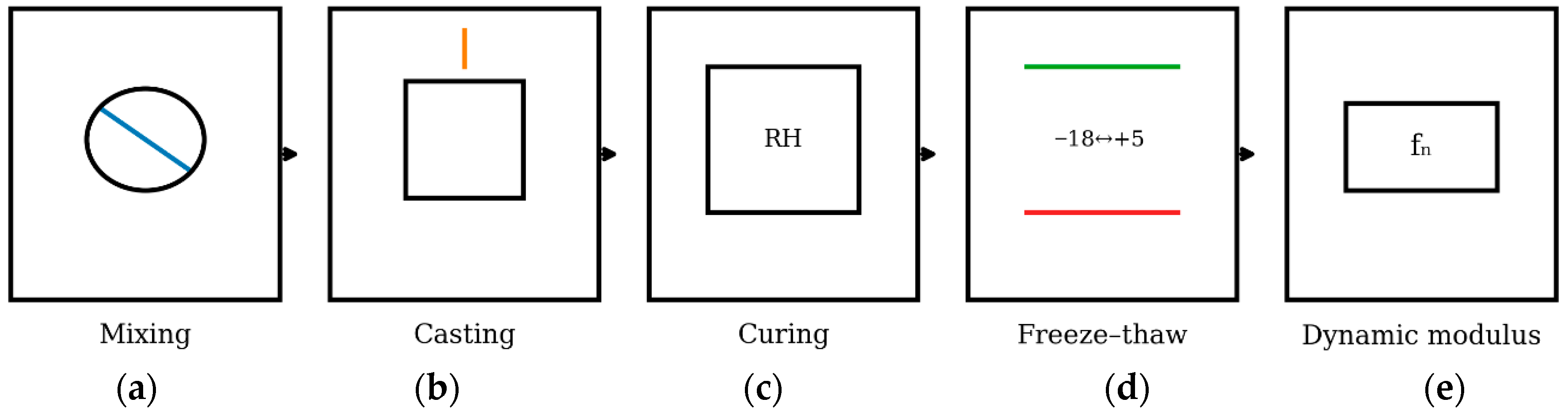
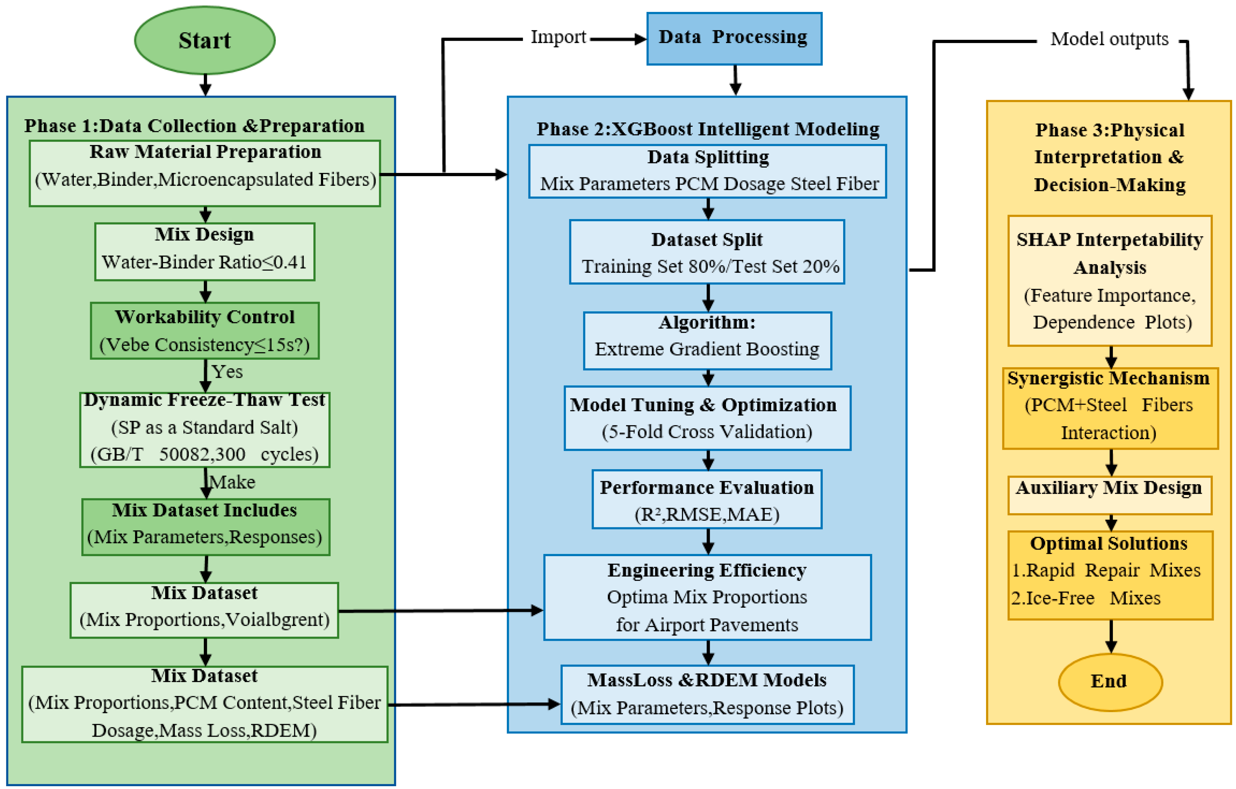
The three-stage research methodology was systematically implemented to ensure a comprehensive and integrated analysis framework, as presented in Figure 1. In the first stage, experimental data collection was conducted to obtain high-quality and reliable datasets representing the physical behaviour of the system under study. The second stage involved the development and training of machine learning models to capture complex, non-linear relationships within the data, followed by a final stage of mechanistic interpretation to explain the underlying physical processes and validate the model outcomes against established theoretical principles.

2.1.2. Aggregates

The coarse aggregate utilised in this research was a continuously graded crushed stone with a maximum nominal particle size of 20 mm. This option meets the load-bearing criteria for airport pavements. It also guarantees compatibility with robotic slip-form paving operations [33]. The fine aggregate was natural river sand with regulated grading (fineness modulus of 2.7) to ensure consistency in workability. Both aggregates complied with the gradation requirements of MH/T 5006-2024 [34] for airport pavement concrete. To maintain a constant total solid volume and prevent unintended variations in density or paste content, fine aggregate was substituted with phase-change material (PCM) on an equivalent mass basis. This approach ensures consistency in mixture proportions while allowing the influence of PCM incorporation to be isolated and accurately evaluated. The gradation curves and key physical characteristics of the aggregates used in this study are presented in Appendix A for reference.

2.1.3. Microencapsulated Phase-Change Material (mPCM)

A core–shell microencapsulated phase-change material (mPCM) is used to control freeze–thaw damage of concrete. It had a phase transition temperature of 0 °C. This temperature was chosen to minimise freezing incidents on the pavement surface [35]. A paraffin-based PCM, forming the core of the microcapsules, plays a key role in regulating temperature gradients and delaying ice formation by absorbing and releasing latent heat during phase transitions. This thermal buffering effect helps stabilise the surrounding environment under fluctuating temperature conditions. The PCM used in this study has a nominal latent heat capacity in the range of 180–200 J/g, indicating its strong heat storage capability [36]. The surrounding polymer shell is composed of melamine-formaldehyde resin, also used in mPCM to enhance structural stability, reduce elastic deformability, and compensate for the hydraulic pressure caused by frost during ice expansion [37]. Due to the soft-shell structure of the PCM microcapsules and the effects of aggregate replacement, high PCM dosages reported in previous studies have been associated with increased porosity and a corresponding reduction in mechanical strength [38,39]. For practical engineering applications, a comprehensive understanding of the interactions between PCM and reinforcing components is essential. Detailed data on the characterisation of the microencapsulated PCM (mPCM) are provided in Appendix A.

2.1.4. Steel Fibres

Copper-coated steel fibres were made to improve crack resistance and counteract any strength loss caused by the addition of PCM. The fibres were 0.2 mm in diameter and 13 mm long, with a length-to-width ratio of about 65. Fracture-bridging methods have been mostly applied to improve freeze–thaw endurance, reduce crack propagation, and increase the tensile load-bearing capability of steel fibre reinforcing [40,41,42]. The copper coating improves the performance of airport pavements over time by providing corrosion resistance in areas where de-icing salts are present [43]. The tensile strength of the fibres was expected to be 2000 MPa or more. The effects of increased reinforcement were systematically assessed at 0%, 0.6%, 0.9, and 1.2 by volume of fibre dosage in the experimental matrix.

2.1.5. Chemical Admixtures

The addition of microencapsulated PCM can dramatically limit workability because of its large specific surface area and tendency to entrap mixing water [44]. According to MH/T 5006-2024 [34], airport paving requires constant rheological behaviour, which is generally determined by a Vebe consistency of 1015 s, in order to achieve slip-form building. A high-performance polycarboxylate superplasticiser (SP) was used as a dynamic rheological adjustment parameter to preserve the same range of workability and water content. The superplasticiser met GB 8076-2008 criteria [21] due to its 40% solid content and water reduction rate of more than 30. The SP dosage was gradually adjusted as the PCM content rose to compensate for water absorption and provide uniform compaction and finishing quality. This approach ensured that variations in fresh-state properties did not inadvertently influence or misrepresent differences in freeze–thaw resistance.
It should be noted that the superplasticiser dosage was slightly adjusted across combinations to achieve uniform workability. Although this introduces a secondary variable, its variation was kept within a narrow range and is not expected to significantly influence freeze–thaw durability compared to the primary factors, namely PCM and steel fibre content. Nonetheless, its possible influence is recognised and constitutes a tiny source of uncertainty in the experimental outcomes.

2.2. Mix Proportion Design

2.2.1. Factorial Experimental Design

The corresponding relationship between PCM-induced heat regulation and steel fibre mechanical reinforcement was systematically studied by methodical means of a full factorial design (FFD). PCM substitution had five types of equal mass (0, 3, 6, 9, and 12). The volume fractions of steel fibre were 4 (0), 6 (0.6), 9 (0.9), and 12 (1.2). This factorial design yields 20 different mixing groups (5 × 4) and helps to quantify the interaction effect of variables in a way that is independent of one another. Because of the reduced stiffness and differing surface properties of PCM particles, this replacement approach is known to affect material density, particle packing, and the properties of the interfacial transition zone (ITZ). However, this method enables the combined thermal and mechanical impacts of PCM to be assessed in a genuine engineering environment. The potential influence of these changes is represented in the measured durability performance and is regarded as a component of material behaviour rather than an independent variable. This kind of systematic variation provides a high-quality dataset to use in further machine learning modelling [45].
The chosen ranges of PCM (0–12%) and steel fibre content (0–1.2%) were calculated using a mix of past research and practical engineering concerns. Existing research has demonstrated that PCM concentrations can provide excellent temperature management without causing severe mechanical property loss [8,13]. Similarly, steel fibre concentrations of up to 1.2% are routinely utilised in cementitious composites to improve crack resistance and toughness while preserving workability and preventing fibre clustering. Furthermore, these ranges were chosen to represent actual mix design limits for airport pavement applications that require both durability and constructability. Higher PCM content or fibre doses may cause issues such as excessive strength reduction, poor workability, or mixing and compaction difficulties. As a result, the chosen parameter space reflects a well-balanced and feasible design range.
All mixes had a 0.29 water-binder ratio to eliminate background variability and ensure conditions of a boundary-controlled system. The airport pavements that are exposed to severe environmental loads need to have a low w/b ratio to ensure a high level of durability and frost resistance [46]. As the aggregate composition (coarse aggregate: 1148.1 kg/m3), binder system (cement: 322.5 kg/m3, fly ash: 86.0 kg/m3, and silica fume: 21.5 kg/m3) remained the same, it was made sure that the dosage of PCM and steel fibres had the sole impact on the differences in the observed freeze–thaw performance. The entire experimental design matrix is presented in Appendix B.

2.2.2. Representative Mix Proportions

Table 1 shows sample proportions of the mix design. The dosages of base materials used in each group were maintained properly (as previously stated). The only changes were to the fine aggregate replacement rate, steel fibre percentage, and superplasticiser dose. Table 1 shows six representative mixtures, with the reference representing 0% PCM and 0% SF, the highest single-doped PCM representing 12% PCM and 0% SF, the highest single-doped fibre representing 0% PCM and 1.2% SF, and two optimal mixtures determined using the predictive modelling framework. This is a structured design that enables experimental comparability and accurate mapping of composition variables to durability performance.

2.2.3. Workability Control Strategy

It is vital to maintain similar workability across all combinations to ensure that no fresh-state qualities interfere with hardened-state durability performance. Increased PCM content resulted in microcapsules with a higher specific surface area, which demanded more water and reduced workability. To neutralise this influence, the dosage proportion of superplasticiser was gradually increased with each mixture while keeping the water-binder ratio constant (0.29). The target workability was a Vebe consistency of 10–15 s, which is necessary in slip-form paving of airport pavement in MH/T 5006-2024 [34].
Trial batches of each mixture were made using various SP dosages until the required Vebe time was achieved. This dynamic adjustment process is reflected in the final SP dosages in Table 1. This was done to ensure that all specimens were uniformly compacted to equal densities and that any freeze–thaw performance discrepancies were due to PCM and fibre effect rather than changes in consolidation quality.

2.2.4. Specimen Preparation and Curing Protocol

The concrete specimens were made in compliance with the requirements of GB/T 50082-2009 [47] and the practice commonly used in the laboratory to prepare the concrete specimens for freeze–thaw test. All dry constituents, including cement, supplementary cementitious materials, fine aggregate, and coarse aggregate, were first mixed together using a forced-action mixer and allowed to mix for about 120 s to achieve uniformity. Gradual introduction of microencapsulated PCM was subsequently done to reduce agglomeration and ensure that the capsules are not ruptured during mixing. The addition of the steel fibres was done gradually and spaced out evenly to prevent fibre balling, and water premixed with the predetermined dosage of polycarboxylate superplasticiser was added. The wet mixing was then maintained for 180 s more until the mixture became homogenous.
The fresh concrete was poured into prismatic-shaped moulds with nominal sizes of 100 mm × 100 mm × 400 mm, which are usually used in relative dynamic modulus testing during freeze–thaw tests. A vibrating table was used to apply compaction to get rid of any entrapped air and to uniformly make the specimen dense. The specimens were then covered with the plastic sheets to avoid moisture loss, stored at a temperature of 20 + 2 °C, after casting.
Upon demolding, all specimens were placed in a controlled curing room maintained at a temperature of 20 ± 2 °C and a relative humidity of at least 95%. They were cured for 28 days to ensure sufficient hydration and microstructural development prior to exposure to freeze–thaw conditions. After the curing, the specimens were placed in water at 20 °C to allow a minimum of 4 days, as per the freeze–thaw testing standard, to reach almost saturated internal moisture conditions. Such a saturation process makes sure that the capillary pores are full of free water to realistically develop hydraulic pressures during freezing cycles. Specimen preparation and testing arrangement are provided in Figure A3 (Appendix F), illustrating the mixing, casting, curing, and testing procedures.
To assess this, the initial mass and basic transverse resonance frequency of each specimen were measured to establish a baseline. These values were then used to calculate the mass loss rate and relative dynamic modulus of elasticity during the freeze–thaw tests. Each mixture group had at least three replicate samples that were tested to guarantee statistical reliability, and the data were analysed as the mean.

2.3. Freeze–Thaw Testing Procedure

2.3.1. Rapid Freezing and Thawing Method

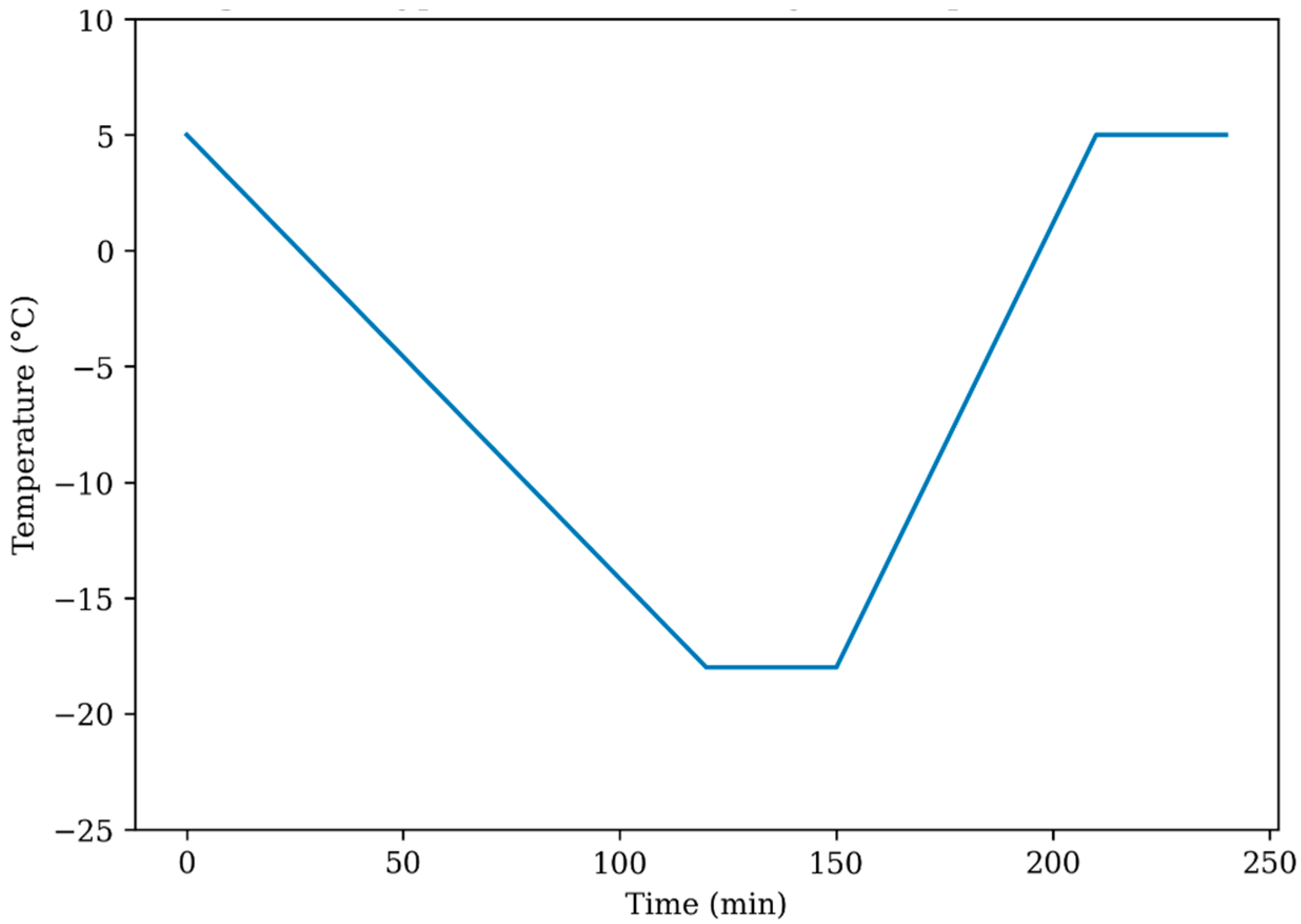
The rapid freezing and thawing method was used to determine freeze–thaw resistance as per the Chinese national standard of GB/T 50082-2009 [47]. It is a well-known method of evaluating the durability of hydraulic concrete under cyclic exposure to freezing. It has been used to model the internal hydraulic pressure of water–ice phase transformation present in the pore structure [48]. Each cycle consisted of a sequence of freezing and thawing, applied to the specimens under controlled temperatures ranging from approximately −18 °C to +5 °C. This temperature range was selected to generate sufficient thermal gradients, inducing the development of internal stresses within the specimens. The standard allowed each full cycle to be finished in 2–4 h. An average temperature pattern during one freeze–thaw cycle is illustrated in Figure A2 (Appendix F), which provides a reference for the thermal loading conditions applied in this study.

2.3.2. F300 Durability Criteria

In order to make engineering relevant, the testing protocol was rigorously benchmarked with respect to the F300 durability requirement of the category 4 airport pavements per MH/T 5004-2024 [49]. The freeze–thaw cycles were set at a maximum of 300, which is the worst exposure category established on civil airport concrete pavements. This limit is associated with the long-term service conditions that are typified by recurring freezing, de-icing chemical encounters, and long-term mechanical loading during aircraft operation. As per the specification, concrete has to have a relative dynamic modulus ≥60% and a loss of mass ≤5% after 300 cycles to be considered an F300 grade.
To confirm the reproducibility of the experimental data, each test point was collected from at least three replicate specimens. The presented values are the average response, with variability defined using the coefficient of variation (CV) and standard deviation. The CV values for both mass loss and RDEM were typically within 5%, indicating high repeatability and low measurement uncertainty.

2.3.3. Damage Indicators: Mass Loss and Relative Dynamic Modulus

Two indicators of durability (e.g., mass loss rate and relative dynamic modulus of elasticity) were assessed at regular intervals to track the progression of damage. Surface scaling and material disintegration caused by cracking, as well as particle detachments owing to freezing, indicate the rate of mass loss. At each measurement interval, samples were removed from the testing instrument, dried on a damp cloth, and weighed with an error of 0.1 g on a balance. Cumulative mass loss was computed as a percentage of initial mass.
The relative dynamic modulus was estimated using resonance-based nonstructural testing (Jinan Testing Equipment IE Corporation, Jinan, China), which assesses internal stiffness deterioration caused by initiating and propagating microcracks. The basic transverse resonance frequency of each specimen was determined, and the RDEM was calculated in the following way:
P =   f n 2 f 0 2   × 100 %
where fn is the basic transverse frequency after n cycles, and fn is the original frequency before exposure to freeze–thaw. A decrease in dynamic modulus is a sign of gradual degradation of the internal load-transfer skeleton, before significant damage occurs to the surface. The sample computations of the mass loss and relative dynamic modulus are detailed in Appendix G.
This experimental setup provides a multiscale deterioration process of steel fibre-reinforced PCM concrete in deplorable freeze–thaw circumstances by concurrently monitoring the parameters of surface and internal damage. The resulting high-resolution durability data offers a solid, reliable, and engineering valuable basis for further machine learning modelling.

2.4. Experimental Database Construction

2.4.1. Boundary-Controlled Conditions

All the experimental factors irrelevant to the research objectives were kept to a minimum in order to achieve a high signal-to-noise ratio and be able to identify PCM–fibre interaction effects without any uncertainty. The boundary conditions were kept constant for all mixtures and test stages (Table 2).

2.4.2. Dataset Structure and Variables

One unique aspect of this study is the analysis of each inspection point as a sample of data, and it is in this way that this traditional endpoint analysis is transformed into a time evolution dataset. Measurements at each of the freeze–thaw stages were recorded as individual entries. The number of completed and consistent records dropped to 145, which constituted the final database, as a few incomplete or inconsistent data points were excluded.
To focus on the major mechanisms determining durability under controlled settings, the model input variables were purposely reduced to three primary components (PCM content, steel fibre content, and freeze–thaw cycles). While freeze–thaw behaviour is intrinsically complicated and impacted by other parameters such as pore structure, air content, and environmental variability, these were controlled in this work to isolate the impacts of the essential design variables.
This streamlined feature space enables a more accurate interpretation of variable interactions while also lowering the likelihood of noise introduction from secondary factors. However, it is recognised that including new properties in future studies may improve model generalisation and application to more complex systems.
The input and output variables were chosen due to their direct significance to freeze–thaw deterioration mechanisms and engineering controllability, as they appear in Table 3 and Table 4.

2.4.3. Data Preprocessing and Partitioning

Before training the model, the dataset was screened using the interquartile range method, and no values exceeding three standard deviations were identified as outliers. This indicates that the controlled experimental conditions produced consistent and reliable data. To ensure numerical stability, all input features were subjected to min–max scaling and brought into the range of [0, 1].
The data was randomly divided into a training sample (80%, 116 samples) and a testing sample (20%, 29 samples) using stratified random sampling based on the freeze–thaw cycles. This categorisation was not influenced by early or late-stage deterioration since the proportional representation of the various levels of degradation in each group was preserved. To thoroughly verify the models’ generalisation and avoid overfitting, the training set was also used in a five-fold cross-validation technique in hyperparameter tuning.
It is important to remember that the dataset is made up of measurements taken at different freeze–thaw stages from the same mix proportions. Because of this, samples from the same mix design may be very similar to each other. The random data partitioning approach employed in this study may cause data from the same mix to be present in both training and testing sets, thus resulting in an overestimation of model performance.
Even though this is a problem, the method used lets the model understand how things get worse over time during freeze–thaw cycles, which is one of the main goals of this study. However, it is noted that this technique largely assesses interpolation capability rather than rigorous extrapolation to unobserved mix designs.
The high-purity, boundary-controlled dataset minimises background noise and emphasises the intrinsic relationships between composition, exposure, and durability. It is carefully designed with a fixed water-to-binder ratio, constant binder composition, uniform curing, and controlled variations only in PCM and steel fibre contents, making it ideal for training a gradient boosting algorithm. This design ensures transparency and repeatability, with the full dataset provided in Appendix C.
A structured validation technique [7] was used to make sure that the machine learning model was reliable and could be used in other situations. First, the dataset was split into a training set (80%) and an independent testing set (20%) at random. This was done using stratified sampling based on freeze–thaw cycles to make sure that both subsets covered all stages of degradation. To keep data from leaking, the testing set was only used for final performance evaluation and was not used during model construction.
Second, during hyperparameter optimisation, the training dataset was put through a five-fold cross-validation process. During this process, the training data were split into five groups. The model was trained on four of these groups and tested on the last one. This method gives a strong approximation of how well the model works and lowers the chance of overfitting to a certain data split.
Finally, we used many statistical measures, such as the coefficient of determination (R2) and root mean square error (RMSE), to assess the model on both cross-validation and independent testing datasets. The fact that the results are the same at all of these evaluation phases shows that the suggested model is strong and can be used in many different situations.

2.5. Machine Learning Methodology

2.5.1. Engineering Trial Mix Database

A high-fidelity engineering database was created using rigorously controlled freezing and thawing experiments carried out under strict boundary conditions. The 20 mix groups were subjected to progressive freeze–thaw exposure for up to 300 cycles, resulting in 145 sets of sequential durability data. Instead of a single terminal-state clinometer, each data point describes a separate freeze–thaw stage of a given combination, capturing the temporal dynamics of degradation. Given its sequential nature, the model can acquire nonlinear propagation rules and cumulative damage behaviour [17].
Input features (Input X) were developed to include three key explanatory variables to ensure physical interpretability and avoid excessive dimensional expansion. One of them is the number of freeze–thaw cycles, which can be used to calculate environmental loading intensity. The second parameter is the volume of steel fibre (SF_Vol), which defines the crack’s bridging capacity. Third, the rate of substitution of phase-change material (PCM_Rep) demonstrates the impacts of heat regulation and microstructural changes. These factors were chosen because they are directly controlled in engineering or because they contribute significantly to frost resistance [11,14].
The output goals (Target Y) included two indications of durability: mass loss rate and relative dynamic modulus of elasticity (RDEM). RDEM exhibits internal stiffness degradation due to microcracking and structural weakening, whereas mass loss is a result of surface scaling and material disintegration [29]. They provide complementary explanations of freeze–thaw damage across a variety of scales.
Outliers were assessed using interquartile range analysis, and no values exceeding three standard deviations were identified, indicating a consistent and reliable dataset. All variables were normalised as needed to guarantee that the training process is numerically stable. To test the model’s generalisation capacity, the dataset was randomly divided into two sets: training (80%) and testing (20%). The splitting was carried out using stratified random sampling to guarantee that both subsets were equally represented in terms of freeze–thaw stages. This method decreases the likelihood of information leakage between training and testing data and eliminates bias in relation to certain stages of deterioration [11].
The database’s internal consistency is adequate due to predetermined material constraints (unchanging w/b ratio, binder system, and curing regime); the total sample size (145) is tiny compared to large-scale machine learning data. Such datasets with boundaries are particularly well-suited to gradient boosting techniques because they frequently have greater signal-to-noise ratios than heterogeneous multi-source datasets [42].

2.5.2. Mathematical Formulation of XGBoost

This section offers the mathematical expression of the XGBoost algorithm in order to gain theoretical rigour and understanding of the optimisation in the context of the predictive framework. XGBoost (Extreme Gradient Boosting) is a descendant of the gradient boosting decision tree (GBDT) methods, which construct predictive models by an iterative process in which all weak learners, often regression trees, are integrated into a single strong ensemble learner [25].
Given a dataset of n samples and m features, the prediction y ^ i of the i-th sample can be written as a sum of K regression trees:
y ^ i = k = 1 K f k x i ,     f k F
where y ^ i is the predicted value (mass loss rate or RDEM), xi is the input feature vector (Cycles, SF_Vol, PCM_Rep), fk represents the k-th regression tree, and F denotes the space of all possible regression trees.
Each tree maps an input vector to a leaf weight:
f k x =   w q ( x )
where q(x) is a function that assigns a sample to a specific leaf node, and w represents the leaf weight (continuous score) associated with that leaf.

2.5.3. Regularised Objective Function

The XGBoost basic idea consists of the minimisation of a regularised objective function that strikes a balance between the accuracy and complexity of the model:
L ϕ = k = 1 n l y i ,   y ^ i + k = 1 K Ω f k
where l y i ,   y ^ i is the loss function measuring the discrepancy between predicted and observed values, and Ω(fk) is the regularisation term penalising model complexity. In regression problems, e.g., prediction of freeze–thaw durability, a squared error loss is generally employed:
l y i ,   y ^ i =   y i   y ^ i 2
The regularisation term is defined as:
Ω f = Υ T + 1 2 λ j = 1 T w j 2
where T is the number of leaf nodes in the tree, wj is the weight of leaf j, γ controls the penalty for additional leaf nodes (tree complexity), and λ is the L2 regularisation coefficient. The formulation prevents overly complicated trees, and it minimises overfitting, which is especially significant when there is a small sample of engineering data, and noise is more likely to be picked up than signal.

2.5.4. Second-Order Taylor Expansion and Split Gain

To efficiently optimise the objective function, XGBoost applies a second-order Taylor expansion of the loss function at iteration t:
L ( t ) i = 1 n g i f t ( x i ) + 1 2 h i f t 2 ( x i ) + Ω ( f t )
where g i = y ^ ( t 1 ) y i , y ^ ( t 1 ) is the first-order gradient, and h i = y ^ ( t 1 ) 2 l y i , y ^ ( t 1 ) is the second-order gradient (Hessian).
For squared error loss:
g i =   y ^ i   y i ,     h i = 2
The optimal leaf weight w j * for leaf j can then be analytically derived as:
w j * =   i I j g i i I j h i + λ
where Ij represents the set of samples assigned to leaf j. Substituting this optimal weight into the objective function yields the gain from splitting a node:
G a i n =   1 2 ( g L ) 2 ( h L + λ ) + ( g R ) 2 ( h R + λ ) ( g ) 2 ( h + λ )   Υ
where
gi: First-order gradient of the loss function with respect to the predicted value at iteration t−1, i.e.,
hi: Second-order gradient (Hessian) of the loss function, i.e.,
gL: Sum of first-order gradients of samples assigned to the left child node after splitting.
hL: Sum of second-order gradients of samples assigned to the left child node.
gR: Sum of first-order gradients of samples assigned to the right child node.
hR: Sum of second-order gradients of samples assigned to the right child node.
g: Sum of first-order gradients of samples in the parent node before splitting.
h: Sum of second-order gradients of samples in the parent node.
λ: L2 regularisation coefficient applied to leaf weights to prevent overfitting.
γ: Structural regularisation parameter controlling the penalty for introducing a new leaf node (model complexity control).
Gain: Improvement in the regularised objective function after performing the split; a positive gain indicates that the split reduces total loss and should therefore be accepted. This split-gain formulation enables efficient tree construction while explicitly controlling complexity.

2.5.5. Suitability for Freeze–Thaw Durability Modelling

XGBoost is particularly well-suited to modelling since it has the following properties of the freeze–thaw degradation process:
Nonlinear cumulative damage: The relationship between cycle number and mass loss indicators (RDEM) may exhibit acceleration or retardation. The XGBoost methodology’s second-order gradient boosting can be utilised to approximate such nonlinear response surfaces without having to define the use of functional forms beforehand.
Combination effects: The combination of PCM heat regulation and steel fibre mechanical reinforcement produces complicated coupling effects that change with exposure intensity. Hierarchical splitting XGBoost has an inbuilt tree-based structure that identifies these correlations, which can then be trained by the model. For example, PCM efficacy can be influenced by both fibre content and cycle number.
Phase-changing materials can produce dosage levels that stabilise or reduce their advantages. As volume fractions increase, fibre reinforcement may yield declining returns. Tree-based approaches that make no parametric assumptions work best for capturing these threshold effects.
Stage-dependent degradation: Increased freeze–thaw cycles can cause interior scaling to replace surface scaling as the primary destructive activity. XGBoost can learn stage-dependent patterns by partitioning the feature space (namely, cycle number) into regions with varying degradation behaviour.
Regularisation with little datasets: The dataset is of moderate size (145 observations). XGBoost’s shrinkage (learning rate), subsampling, and intrinsic L1 and L2 regularisation are effective in reducing overfitting while maintaining predictive accuracy. All of these lead to XGBoost serving as the best algorithmic basis for the proposed structure’s freeze–thaw life prediction in controlled boundary conditions.

2.5.6. Model Training and Hyperparameter Optimisation

To boost generalisation performance, the model was trained using a five-fold cross-validation method [28]. A five-fold cross-validation technique was used to improve model generalisation and ensure effective evaluation. The training dataset (116 samples) was randomly divided into five roughly equal sections. Each cycle used one subset for validation and four subsets to train a model. The validation set for each subgroup was used once during the five iterations of this process. Cross-validation performance was evaluated as the average of the five validation scores. Candidate configurations are tested on a variety of validation sets to identify which configurations produce the lowest prediction errors.
The Root Mean Square Error (RMSE) served as the major cross-validation testing metric. RMSE was chosen because it penalises significant deviations more than the Mean Absolute Error. It is also commonly utilised in durability modelling research [13].
RMSE is defined as:
R M S E =   1 n i = 1 n y i   y ^ i 2
where yi and y ^ i are the observed and predicted values, respectively.

2.5.7. Hyperparameter Tuning

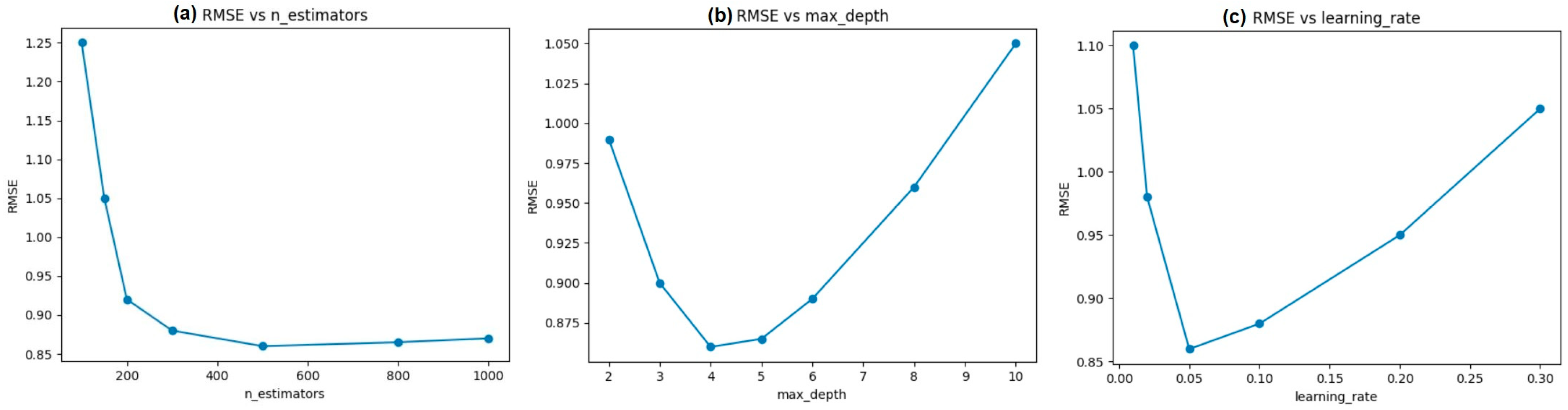
Hyperparameterisation was performed using a grid search approach [29] with a five-fold RMSE from cross-validation and an objective assessment metric. One of the hyperparameters examined was the number of base learners (n-estimators). This regulates the regularisation coefficient, sparsity, model complexity, boosting iterations, tree contributions, tree complexity, robust randomness, and overfitting to tiny subsets [29]. The most effective setup for reducing cross-validation RMSE was identified after thorough research; the final hyperparameters for the XGBoost model are shown in Table 5.
The selected parameter ensures high accuracy of prediction without any loss of the generalisation capacity by finding the optimal compromise between bias and variance. The model can be expanded slowly as it is stable due to its low learning rate (0.08) and a relatively high number of estimators (450). The fact that the sample size used is medium makes the explicit control of the model complexity offered by the L1 and L2 regularisation terms (α = 0.1, λ = 1.0) highly important. The subsample (0.8) and the column sampling (0.8) parameters make use of randomness that enhances solidarity and reduces the connection between trees.
The retraining of the final model was done on the entire training data (116 samples) at the optimum setup after hyperparameter optimisation. The true generalisation ability of the trained model was then evaluated against the independent testing data, which comprised 29 samples. Findings of the hyperparameter search space and cross-validation performance of each combination tested are given in detail in Appendix D.

2.5.8. SHAP for Model Interpretability

In order to address the fact that the widespread criticism of ensemble learning models is that they are black boxes, SHAP (Shapley Additive Explanations) analysis was incorporated into the model. SHAP offers a coherent way to explain how model predictions can be interpreted by attributes’ contribution values to each feature according to the cooperative game theory [14].

2.5.9. Game-Theoretic Foundation

The Shapley value of feature j has been defined as the mean marginal contribution of feature ϕj to any coalition of features:
ϕ j =   S F / { j } S ! F S 1 ! F ! [ f S x S j     f S x S ]
where F is the set of all features, S is a subset of features not including feature j, fS is the model prediction conditioned on the features in subset S, and xS{j} is the prediction when feature j is added to subset S. The combinatorial weight accounts for the number of ways to form coalition S.
In the case of tree-based models, including XGBoost, SHAP has an effective approximation algorithm (TreeSHAP) that uses tree structure to compute Shapley values in cubic time instead of exponential time [38].

2.5.10. SHAP Values for Feature Attribution

SHAP analysis achieves several interpretability goals in this paper. To provide a ranking of feature contributions that takes into account both the size and frequency of influence, it first calculates global feature relevance by averaging absolute SHAP values across all samples. This enhances the feature significance metrics built into XGBoost. Second, SHAP employs signed values to facilitate the generation of directorial impact analysis: the higher the SHAP value, the greater the feature’s effect on the prediction, and vice versa. For example, a negative SHAP indicates that more freeze–thaw cycles diminish the predicted modulus (deleterious effect), whereas a positive SHAP indicates that an increasing dose of steel fibre content results in an increase in the relative dynamic modulus. Third, SHAP interaction values break down the contributions of main and interaction effects between pairs of features, allowing for a quantitative assessment of the synergistic effect of PCM and steel fibres under successive freeze–thaw stress. Fourth, SHAP describes particular predictions: SHAP values express the difference between a single forecast and the baseline in terms of certain feature values [28,29]. The SHAP analysis was carried out using the SHAP library (Version 0.41.0, available at https://github.com/slundberg/shap, accessed on 6 April 2026) implemented in Python (Version 3.10, Python Software Foundation, USA). The TreeExplainer method, specifically designed for tree-based models, was employed to interpret the predictions of the XGBoost model (Version 1.7.6, available at https://xgboost.readthedocs.io/, accessed on 6 April 2026). The outputs include SHAP summary (beeswarm) plots, which show the distribution of SHAP values for each feature across all samples, with different colours reflecting the size of a feature. SHAP force plots illustrate the contribution of each feature to each prediction, whereas SHAP dependence plots indicate the influence of a feature’s SHAP value on its value, as well as potential interaction effects with other features. The present approach reveals the underlying thermomechanical synergistic mechanisms impacting frost resistance, in addition to providing high-precision prediction via XGBoost and SHAP. This interpretability is required to foster trust in AI-based decisions, which might be valuable in safety-critical infrastructure such as airport pavements.

3. Results

3.1. Experimental Observations of Freeze–Thaw Deterioration

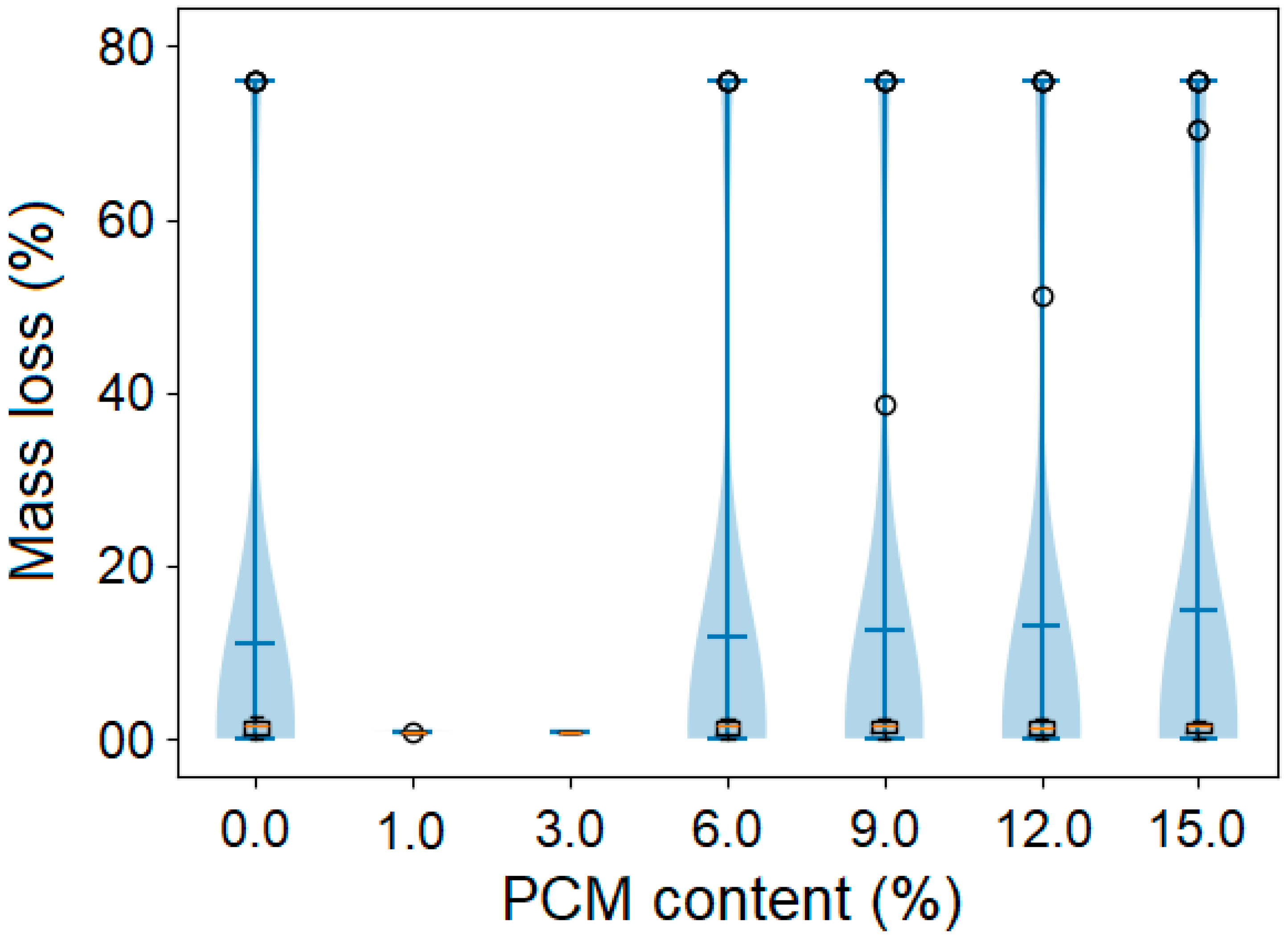
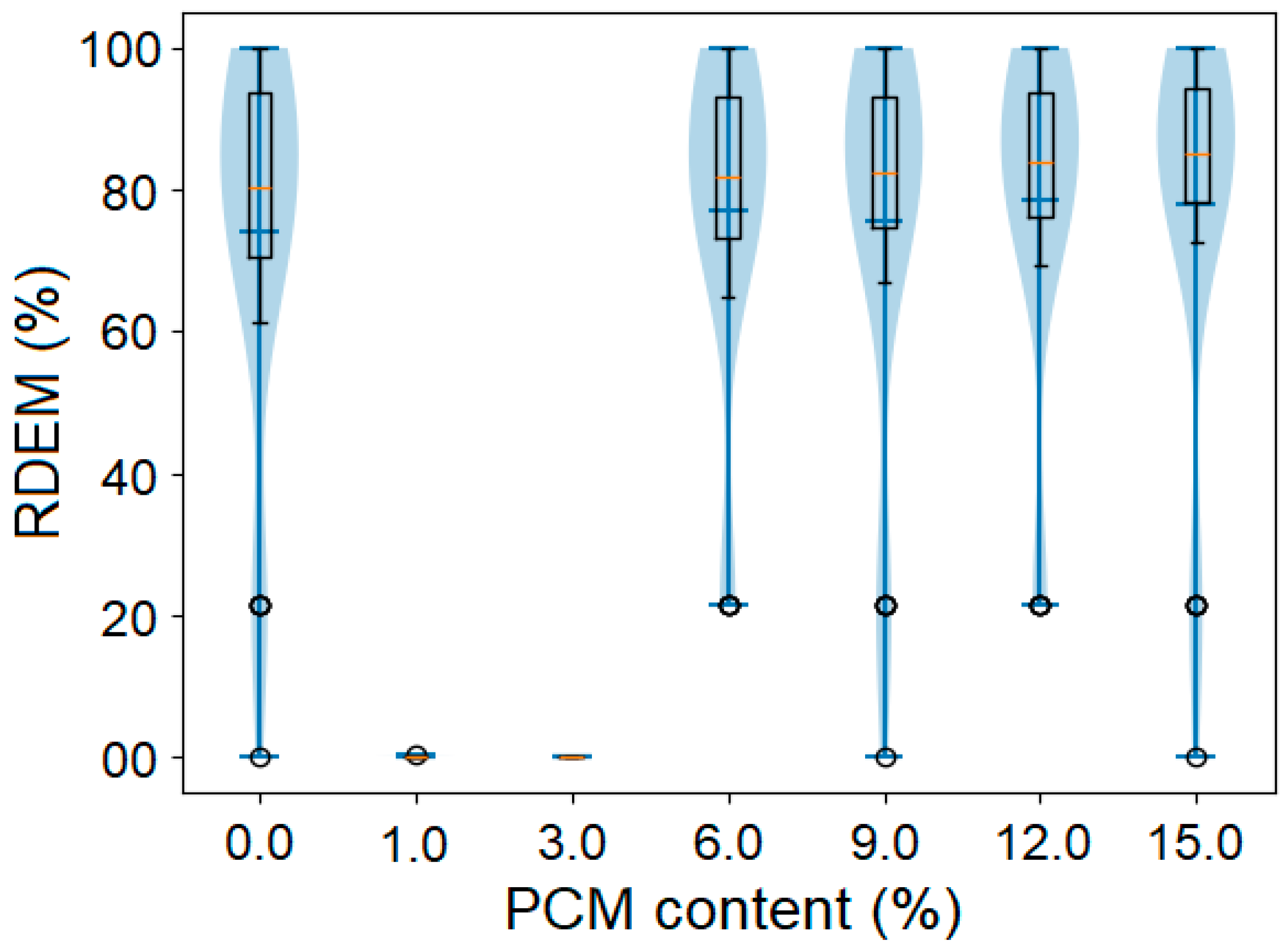
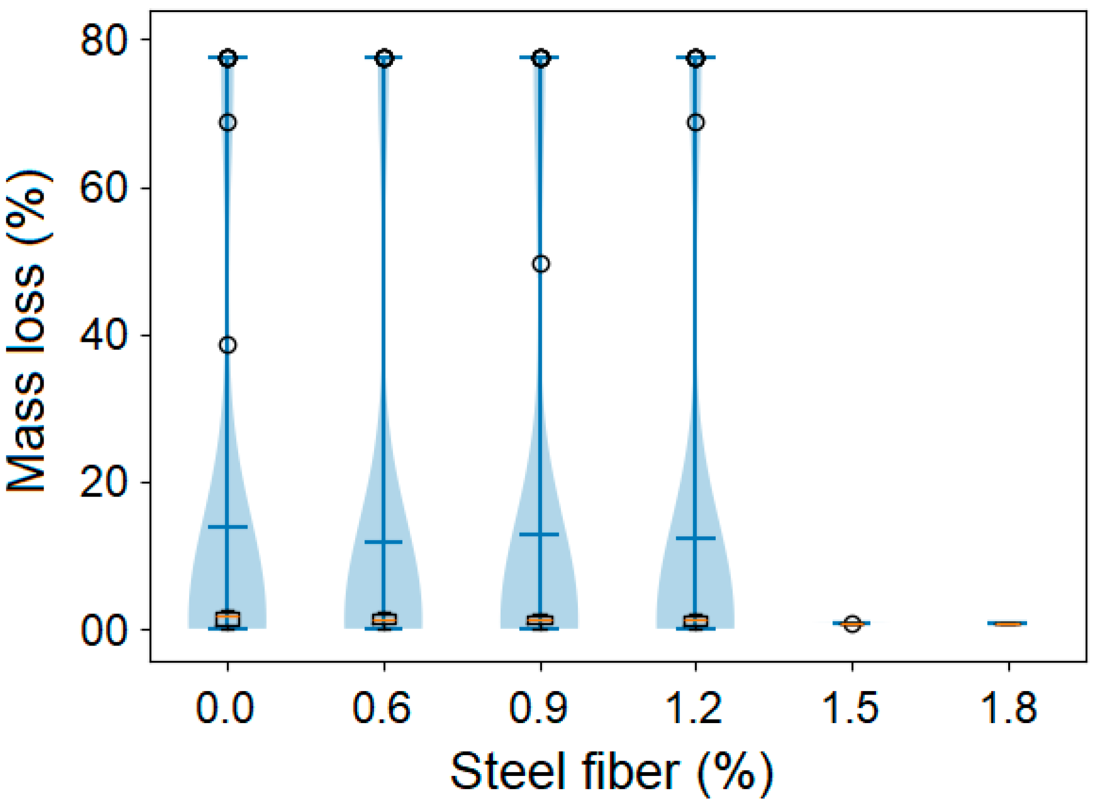
Freeze–thaw deterioration of steel fibre-reinforced phase-change concrete of the concrete was systematically observed through loss in mass and relative dynamic modulus measurements at periodic intervals up to the point of 300 cycles. The experimental results showed that there were unique deterioration trends depending on PCM content, as well as the dosage of steel fibre (Figure A4 (Appendix F)). In addition to the mean values, the variability of the measurements was investigated in order to determine statistical reliability. The comparatively low standard deviation and coefficient of variation reported among repeated specimens suggest that the experimental results are reliable and repeatable. This validates the reported freeze–thaw performance trends across various mix settings. Representative deterioration patterns after 300 freeze–thaw cycles are shown in Figure A4 (Appendix F), providing visual evidence of surface damage and material degradation under different mix configurations.

3.1.1. Mass Loss Evolution

In all mixtures, mass loss, which measures surface scaling and material breakdown, increased gradually with freeze–thaw cycles. Nonetheless, the material’s composition had a significant influence on the mass loss rate and quantity. The reference combination (0% PCM, 0% SF) was the most degraded, with a mass loss of 2.45, which was close to the F300 specification threshold of 5, but still within acceptable limits. Mass loss was also decreased to 2.12% by PCM alone at 12%, representing a 13.5% improvement over the reference. The given enhancement is related to PCM’s thermal regulation effect, which minimises the severity of strains encountered during freezing and softens internal temperature gradients.
Steel fibre reinforcement alone at 1.2% proved to be more effective, reducing mass loss to 1.98–19.2% less than average. The capacity of steel fibres to fill cracks avoids the formation of microcracks and their coalescence to generate spalling on the surface, which explains their excellent performance. The most significant improvement was noticed in compounded combinations. Although the extreme-performance configuration (12% PCM + 1.2% SF) reduced mass loss to 1.87, a 23.7% improvement over the reference, the economical design (9% PCM + 0.9% SF) performed best, with a mass loss of 1.95.
Interestingly, the growth of mass loss in all mixes follows a three-stage pattern, with a sluggish buildup period (0–100 cycles), an enhanced degradation phase (100–250 cycles), and final stability (250–300 cycles). This pattern demonstrates the damage induced by freeze–thaw as progressive, with initial microcrack formation increasing over time to a critical point in terms of surface spalling.

3.1.2. Relative Dynamic Modulus Degradation

The relative dynamic modulus of elasticity (RDEM) is a sensitive indicator of internal stiffness deterioration, which has been linked to microcrack formation and propagation inside the cementitious matrix. RDEM degradation, like mass loss, was found to be substantially dependent on PCM and steel fibre composition.
By 300 cycles, the RDEM of the reference mixture had gradually decreased to 61.2, slightly higher than the minimum of 60 at F300 standard. This demonstrates that the reference concrete operates with a moderate safety margin despite the fact that it barely meets the durability requirements. At 300 cycles, the RDEM had increased to 72.6% with the addition of 12% PCM and 74.3% steel fibres alone. Steel fibres’ exceptional performance reflects their mechanical significance in maintaining structural integrity through stress redistribution and microcrack bridging.
The combined arrangements demonstrated a lot of synergy. The 9% PCM + 0.9% SF mixture retained 79.4% and 66.8% of the RDEM after 200 and 300 cycles, respectively. The reference had the highest residual stiffness after 300 cycles, with an RDEM of 72.6% − 18.6% higher than the reference, and the extreme-performance configuration (12% PCM + 1.2% SF). This improved performance indicates that better resistance to internal damage buildup is obtained by the thermomechanical interaction of PCM temperature regulation and steel fibre mechanical reinforcement.
The RDEM degradation curves show that the protective action of PCM and steel fibres is most pronounced at the intermediate and late stages of freeze–thaw exposure (more than 150 cycles), implying that both materials are particularly useful in slowing the formation of microcrack networks once they have emerged.
To evaluate statistical dependability, the variability of the experimental outcomes was closely studied in addition to the average trends. At least three duplicate specimens were evaluated for each mixture and measurement point, and the reported data provide the average response. For both mass loss and RDEM, the coefficient of variation (CV) was generally less than 5%, suggesting low experimental dispersion and strong repeatability.
The tightly regulated boundary conditions used in this investigation, such as a constant water-binder ratio, a uniform curing regime, and consistent workability control, are responsible for the comparatively low variability. These circumstances reduce external sources of variability and guarantee that PCM and steel fibre contents are the main factors influencing the observed variations in durability performance. As a result, the trends found in this investigation can be regarded as reflective of the intrinsic material behaviour and statistically reliable.
The claimed best performance at specified PCM and steel fibre contents can be explained using thermomechanical and microstructural principles. PCM improves thermal control by absorbing and releasing latent heat near the freezing point, which reduces temperature variations and limits ice formation inside the pore structure. This helps to reduce internal hydraulic and osmotic pressures during freeze–thaw cycles. However, increasing PCM content creates soft inclusions, which can increase porosity and weaken the interfacial transition zone (ITZ), lowering mechanical integrity. As a result, there exists an ideal PCM range that maximises thermal benefits while minimising microstructural damage.
Steel fibres address this constraint by increasing crack resistance and ensuring structural continuity. Fibres use fracture-bridging mechanisms to limit microcrack propagation and delay crack coalescence under cyclic stress, increasing resistance to stiffness degradation and mass loss.

3.2. Model Performance Evaluation

3.2.1. Comparative Assessment of ML Algorithms

Several well-known regression models were used as a baseline in the comparison study to ensure methodological rigour and support the selection of XGBoost as the primary predictive model. They comprised Artificial Neural Networks (ANNs), Random Forest (RF), Support Vector Regression (SVR), and Linear Regression (LR). To ensure a fair and unbiased comparison, all models were trained under identical settings, with the same dataset split (80% training, 20% testing), input features (Cycles, SF_Vol, PCM_Rep), and performance measures.
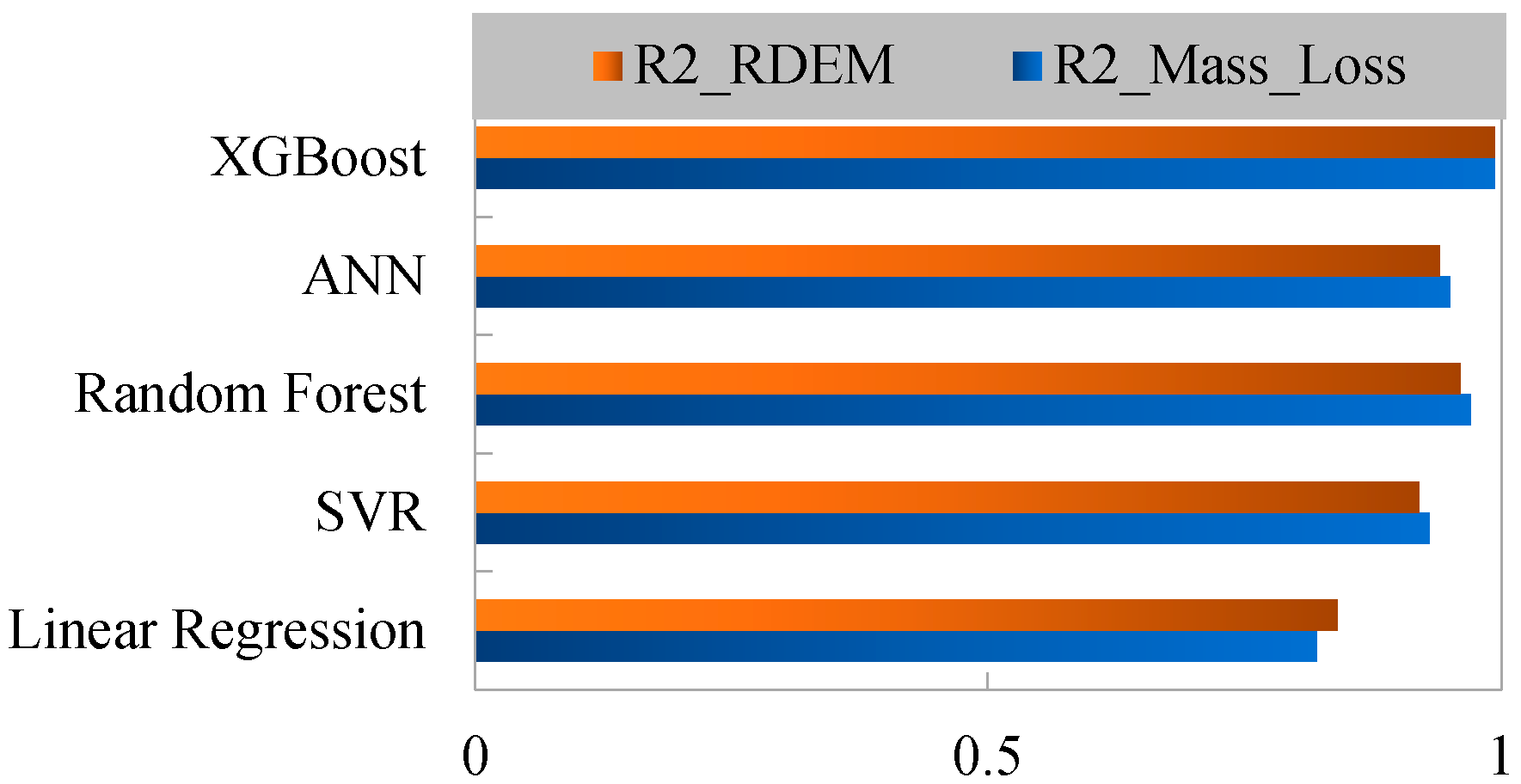
Linear Regression had the lowest accuracy, with R2 values of 0.82 for mass loss and 0.84 for RDEM. This poor performance demonstrates that nonlinear developments in the freeze–thaw degradation process cannot be properly explained by linear assumptions. Nonlinear modelling approaches are important because of the deterioration processes that include progressive microcrack development, nonlinear damage development, and complicated interactions between PCM and steel fibres (Table 6).
Support Vector Regression and Artificial Neural Networks showed improved prediction power, with R2 values ranging from 0.92 to 0.95. Nonetheless, the comparably small sample size of those experimental datasets containing boundaries, as well as the impacts of nonlinear interactions between PCM and steel fibres, continued to have an impact on performance. Regularisation was ineffective in ANN, which is prone to overfitting due to the training of sophisticated neural structures on large datasets (Table 6).
Random Forest also improved prediction accuracy, with R2 values of 0.97 and 0.96 for mass loss and RDEM. This improvement demonstrates the natural advantage of ensemble learning approaches in explaining complex, nonlinear degradation behaviour using feature randomisation and bootstrap aggregation. However, Random Forest’s prediction error (RMSE = 2.53 for RDEM and 0.124 for mass loss) was significantly higher than that of XGBoost.
The XGBoost model outperformed all baseline strategies, achieving R2 values of 0.9938 for mass loss prediction and 0.9935 for RDEM prediction (Figure 2). Among all the models studied, the mass loss was 0.0957, and the RDEM was 0.9687. This superior predictive capability is due to XGBoost’s inherent algorithmic benefits, which include second-order Taylor expansion of the loss function to compute accurate gradient optimisation, explicit L1 and L2 regularisation to help control model complexity and avoid overfitting, and built-in support for missing values to improve robustness when using small to medium engineering datasets. Furthermore, XGBoost showed competitive training performance and was capable of producing significantly higher accuracy at a much lower computation time than ANN.
Among the evaluated models, XGBoost demonstrated the best predictive performance in this study, achieving higher accuracy compared to the other algorithms under the same dataset and evaluation conditions (see Figure 2). This can be attributed to its ability to capture nonlinear relationships and incorporate regularisation, which is particularly advantageous for structured datasets of moderate size.
It should be noted that the high prediction accuracy is achieved within a relatively small but highly controlled dataset, which may contribute to reduced variability and improved model fitting.

3.2.2. XGBoost Prediction Accuracy

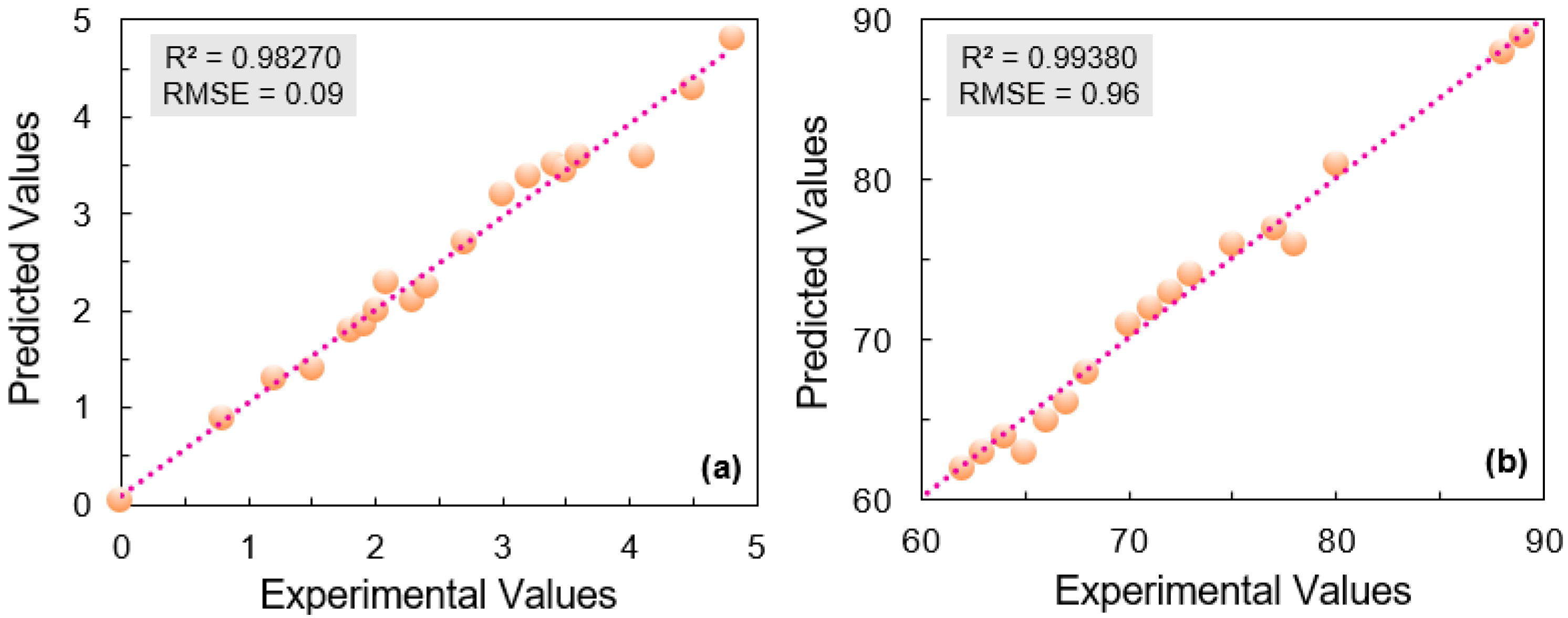
Figure 3 shows that the projected values for both durability indicators using the XGBoost model are very consistent with the experimental values. Scatter points for mass loss rate are practically on the ideal diagonal line (y = x), indicating a very exact prediction across the entire spectrum of deterioration (Figure 3a). The coefficient of determination (R2) is close to 0.9935 even at the freeze–thaw stages, with an RMSE of 0.0957, indicating that the prediction error is low. Figure 3b shows the relative dynamic modulus of elasticity (RDEM); the data points are virtually identical to the ideal fit line, with an R2 of 0.9938 and an RMSE of 0.9687. The proposed model accurately captures the nonlinear cumulative damage characteristics of steel fibre-reinforced PCM concrete up to 300 freeze–thaw cycles, with minimal dispersion and no systematic departure. Technically, the typical F300 durability tests need a significant amount of energy and take approximately three months in the laboratory. In contrast, with the parameters of mix design and target cycle number, the suggested XGBoost-based system can forecast freeze–thaw damage indices within milliseconds. This is due to digital transformation, which removes the typical time constraints in cold-region concrete research and applications, significantly accelerating the decision-making process for airport pavement design.
The exceptional predictive accuracy shows substantial practical significance of this research. Traditional F300 durability testing takes about three months in the laboratory, consumes a significant amount of energy throughout the freeze–thaw cycle, and requires extensive preparation and measurement of specimen samples. In contrast, the proposed XGBoost-based model predicts freeze–thaw damage indices in milliseconds using only mix design specifications and the target number of cycles. Because of this digital shift, making decisions about airport pavement design now takes a few seconds rather than months, as it did in traditional cold-region concrete study and application.
It should be noted that the high prediction accuracy (R2 ≈ 0.99) is achieved within a controlled experimental dataset with limited variability. As discussed in Section 2.4.3 and Section 4, this performance reflects strong interpolation capability rather than unrestricted generalisation. Potential sources of overestimation, such as data correlation and limited dataset size, have been acknowledged and discussed accordingly.

3.2.3. Synergistic Performance of PCM–Steel Fibre Combinations

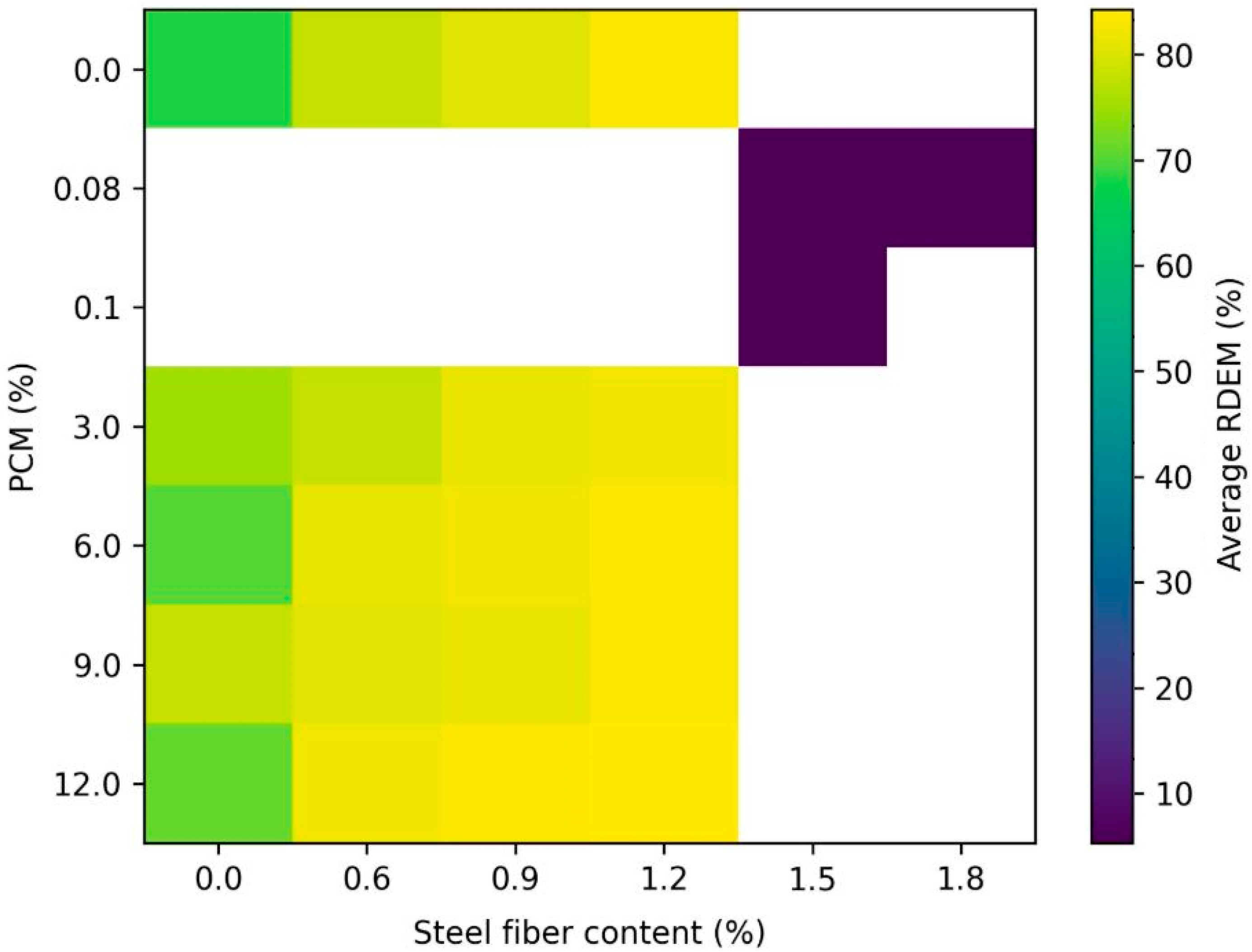
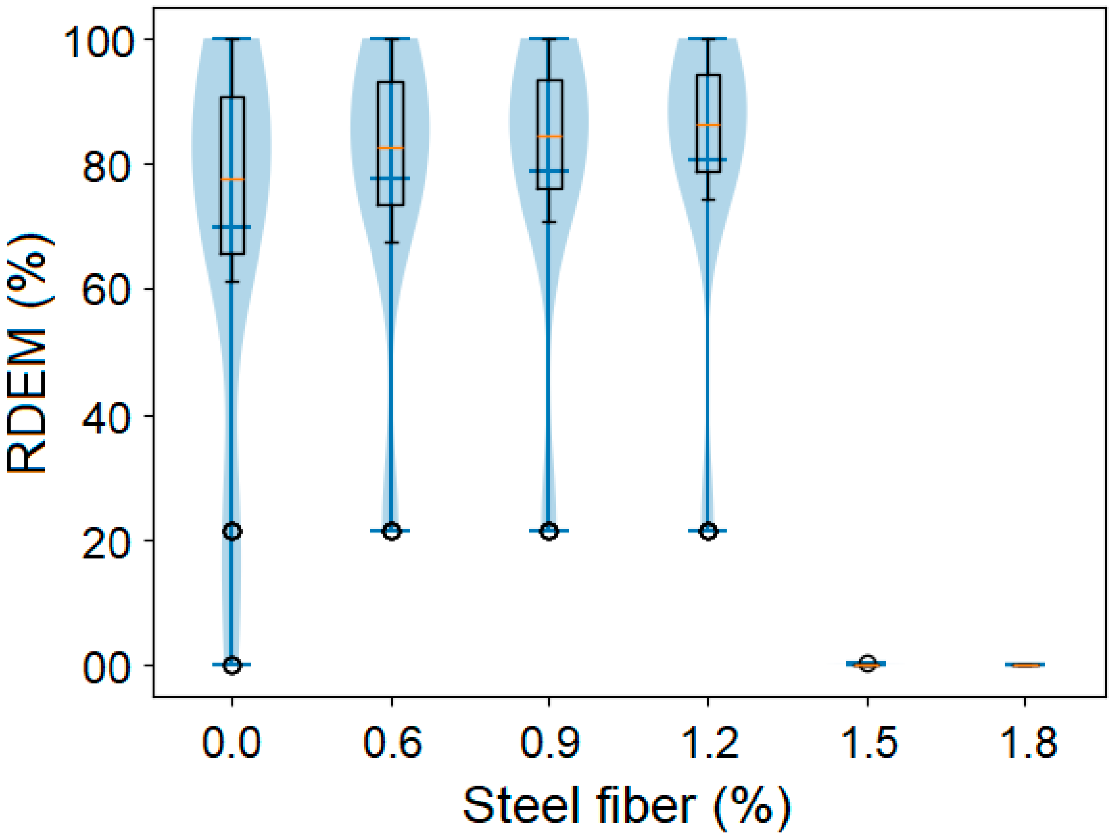
A heatmap visualisation was created to show the average relative dynamic modulus (RDEM) of various material combinations in order to study the overall influence of PCM substitution and steel fibre reinforcing on freeze–thaw durability (Figure 4). The heatmap vibrantly depicts how the two design parameters interact to shape the durability performance.
As demonstrated in Figure 4, the higher the steel fibre concentration, the higher the RDEM value, indicating more resistance to internal stiffness loss during freezing and thawing. This tendency validates the strengthening role of steel reinforcement fibres in terms of crack containment and the preservation of the cementitious matrix’s load-transfer system. Similarly, while managing internal temperature variations during freezing occurrences, higher PCM replacement levels increase durability performance. The PCM–steel fibre combinations have the best RDEM values, indicating a strong synergistic effect of mechanical reinforcing processes and thermal regulation.
Figure 4 also shows that mixtures incorporating fibre reinforcement along with moderate-to-high PCM content exhibit the highest and most consistent durability performance. This finding supports the optimal mixture designs identified through SHAP analysis and machine learning predictions. This image is thus another indication of the thermomechanical coupling mechanism that govern freeze–thaw resistance in steel fibre phase-change concrete.

3.2.4. Residual Analysis and Model Robustness

To provide a more comprehensive evaluation of model performance, residual analysis was conducted in addition to standard metrics such as R2 and RMSE. The robustness of the model was further evaluated based on the validation strategy described in Section 2.4.3. Training and testing predictions have all undergone a residual analysis to determine the reliability of the model. This model satisfies the assumptions of homoscedasticity and independence, as confirmed by the residual plots. No discernible patterns or trends were observed, and the differences between predicted and actual values were randomly distributed across the graph. The residuals were approximately normally distributed with mean values near zero (−0.002 in the case of mass loss, and −0.12 in the case of RDEM), with no outliers exceeding three standard deviations.
The cross-validation results indicated that the five folds were consistent. In the case of mass loss and RDEM, the mean R2 of cross-validation was 0.991 and 0.990, respectively, and the standard deviation was 0.002 and 0.003. The high quality of generalisation of the model is already justified by the fact that the variance between folds is very low, which indicates that the model is stable and is not overly reliant on specific data partitions.
The sensitivity study also established the strength of the model when it was demonstrated that the model remained stable even in cases where the input features were varied slightly. This is particularly important in the case of engineering, where the input parameters might possess inherent measurement uncertainty.
The high prediction accuracy (R2 ≈ 0.99) may indicate overfitting, especially given the limited sample size. However, this performance is mostly due to the experimental database’s high quality and boundary control. Unlike earlier research, which used heterogeneous multi-source datasets, all samples in this work were created under strictly controlled conditions, such as a constant water-binder ratio, identical curing regime, and uniform aggregate system [3,4,5,6]. This considerably decreases background noise while increasing signal-to-noise ratio, allowing the model to learn the fundamental correlations between input variables and durability indicators more efficiently.
Furthermore, several measures were used to reduce overfitting. These include (i) five-fold cross-validation during hyperparameter optimisation, (ii) the application of regularisation techniques within XGBoost (L1 and L2 penalties), (iii) randomisation is introduced through subsampling and column sampling, and (iv) evaluation on an independent testing dataset. The consistency of training, cross-validation, and testing results demonstrates that the model detects generalisable patterns rather than noise.
The residuals are generally small and randomly distributed around zero, with no clear systematic bias observed. This indicates that the model predictions are well-balanced across the range of values and that errors are not concentrated in specific regions of the dataset. The absence of significant skewness or clustering in the residual distribution further supports the reliability of the model.
Nonetheless, it is noted that additional validation using larger-scale or field datasets would be advantageous in fully confirming the model’s durability under more general engineering situations. This issue will be resolved in future development.

3.2.5. SHAP-Based “Thermal-Mechanical” Synergistic Frost Resistance Mechanism of Pavement

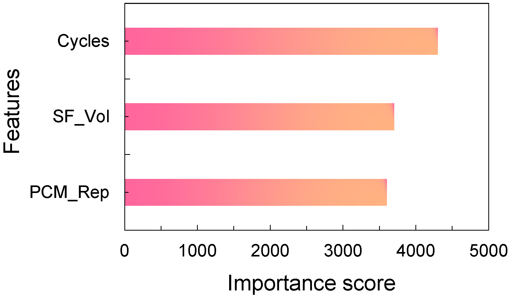
The relative importance of each input variable in predicting the relative dynamic modulus under freeze–thaw cycles was quantified using feature importance analysis, as illustrated in Figure 5. The results indicate that the number of freeze–thaw cycles is the most critical factor, highlighting that cumulative environmental loading primarily drives pavement concrete degradation. The steel fibre volume fraction (SF_VOL) ranks second, contributing significantly to stiffness retention through energy dissipation and crack-bridging mechanisms, while the phase-change material substitution rate (PCM_Rep), though a smaller modification, still plays an important complementary role by regulating temperature and enhancing frost resistance. The hierarchical ranking (Cycles > SF_VOL > PCM_Rep) indicates that pavement durability under F300 conditions is governed by a coupled thermomechanical mechanism. Steel fibres enhance structural integrity, PCM moderates temperature-induced stress variations, and environmental loading dictates the overall degradation pattern. In addition to standard empirical evaluation, this mathematical explanation adds mechanical insight.
The second most important number is the volume fraction of the steel fibre (SF_Vol), which has a mean value of 2.36 (Figure 5), indicating that it plays an essential mechanical function in reducing stiffness deterioration through energy dissipation and fracture bridging. Steel fibres are the major structural protection layer against internal damage from freeze–thaw cycles, according to this quantitative evaluation.
A mean value of 1.84 for the phase-change material substitution rate (PCM_Rep) implies that heat regulation is critical, even if its influence on frost resistance is complementary and less substantial. Under the hierarchical ranking (Cycles > SF_Vol > PCM_Rep), a highly linked thermomechanical process determines pavement integrity at F300 conditions: steel fibres improve structural integrity, PCM controls temperature-induced stress fluctuations, and environmental loading determines the degradation framework.
The same order of ranking was found in mass loss prediction, with cycles coming in first (mean |human| = 0.68), followed by SF_Vol (0.31) and PCM_Rep (0.24). In comparison to RDEM, the protective characteristics of PCM appear to be stronger in preserving internal structural integrity and less severe in deterring surface scaling since PCM’s involvement in influencing mass loss is not as prominent. This discrepancy is consistent with the process of internal heat regulation rather than surface protection, as shown in PCM.

3.2.6. SHAP Summary Plot

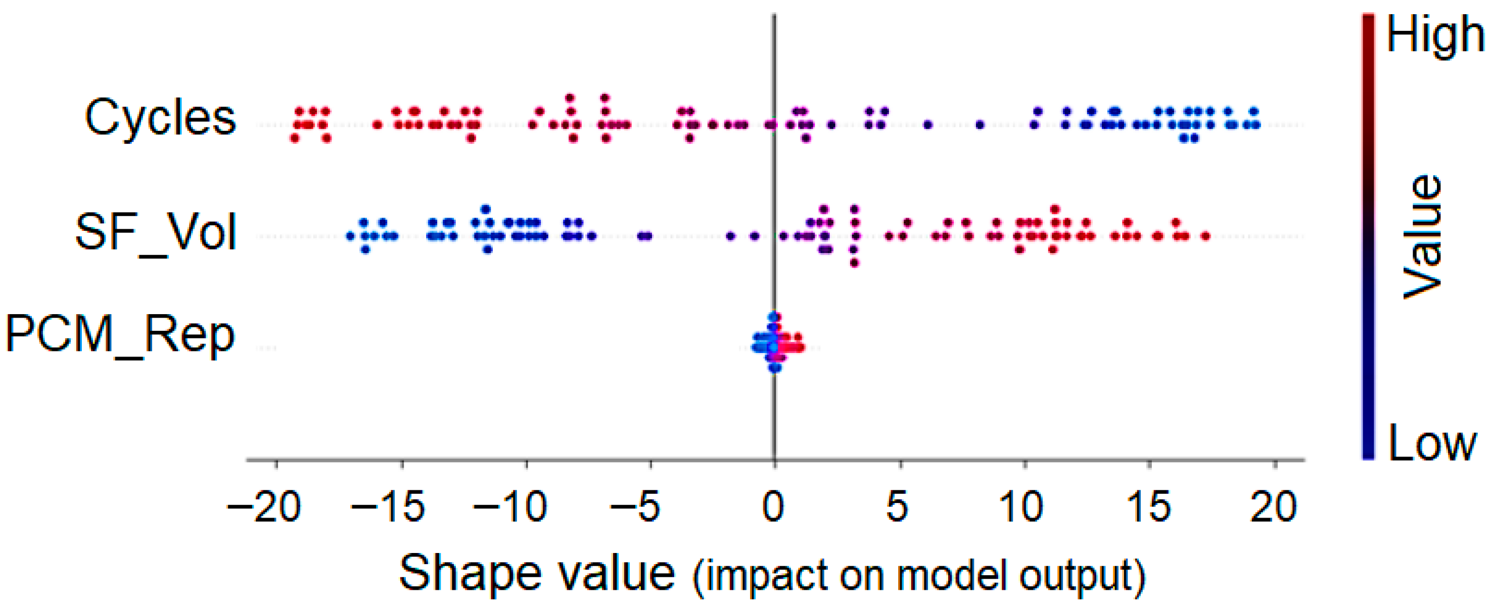
Figure 6 shows the SHAP summary (beeswarm) graphic, which provides a detailed description of the influence of each attribute on the forecast value of the relative dynamic modulus expected. Colour gradients show feature values (blue low, red high), whereas horizontal distributions of SHAP values represent the value and direction of each variable’s contribution to model output. The freeze–thaw cycle number (Cycles) has the highest SHAP distribution, indicating that it plays a significant role in stiffness deterioration. The larger the cumulative freezing-thawing damage, the higher the number of cycles (red dots) associated with negative SHAP values, suggesting a significant fall in the anticipated modulus (Figure 6). On the other side, the modulus forecast contains fewer cycle numbers (blue points).
Increased fibre contents (red points) largely result in positive SHAP values, indicating that they are effective at reducing stiffness loss through crack-bridging and stress redistribution mechanisms. The volume fraction of steel fibre (SF Vol) has a substantial positive correlation with the model result. Conversely, low fibre content is typically associated with poor durability performance.
The SHAP values of PCM substitution rate (PCM_Rep) are more concentrated around the zero value, indicating a moderate but consistent impact. Because of the thermal buffering effect, which reduces internal freeze–thaw stresses, greater quantities of PCM slightly improve durability projections.
The SHAP analysis reveals the presence of a thermomechanical synergistic process: PCM is utilised for heat regulation, steel fibres for structural reinforcement, and environmental stress (cycles) for maintaining degradation levels. This explanatory model improves the physical soundness of the XGBoost model under the supplied F300 engineering boundary constraints.
The freeze–thaw cycle number (cycles) has the highest SHAP distribution, indicating that it plays a substantial role in stiffness deterioration. The relationship between cumulative freezing–thawing damage and number of cycles (red points) is mostly between negative SHAP values, which indicate a significant reduction in anticipated modulus. SHAP values for cycles range from −8 to +2, with negative values increasing as the number of cycles increases. Such a monotonically negative correlation is consistent with the scientific reality that internal damage increases with each subsequent freeze–thaw cycle.
Smaller numbers of cycles (blue dots), which represent the minimum condition of damage during the initial exposure stages, are positively connected with modulus prediction. The model effectively learned the nonlinear damage accumulation rule that propagates freeze–thaw damage, as evidenced by the distinct separation of the high-cycle (red) and low-cycle (blue) terms.
The model output shows a clear positive association with the steel fibre volume fraction (SF_Vol). Higher fibre content (red points) typically results in positive SHAP readings. It demonstrates how steel fibres can effectively minimise stiffness loss due to stress redistribution and crack-bridging mechanisms. Low fibre levels (blue dots) typically result in negative SHAP values, indicating poor durability performance. The SHAP distribution of SF_Vol is rather diffused, indicating that there is no total additivity of fibre contribution, but rather an interaction with other parameters, particularly cycle number, at which the benefits of fibre ingestion become more obvious as deterioration develops.
The summary plot of the SHAP distribution of mass loss revealed directional patterns (similar to those seen in mass loss), with PCM_Rep, SF_Vol, and Cycles contributing positively but moderately and negatively. Importantly, the protective advantages of SF_Vol and PCM_Rep on mass loss were slightly smaller when compared to RDEM effects, demonstrating that these materials are more successful at retaining internal stiffness than preventing surface scaling.

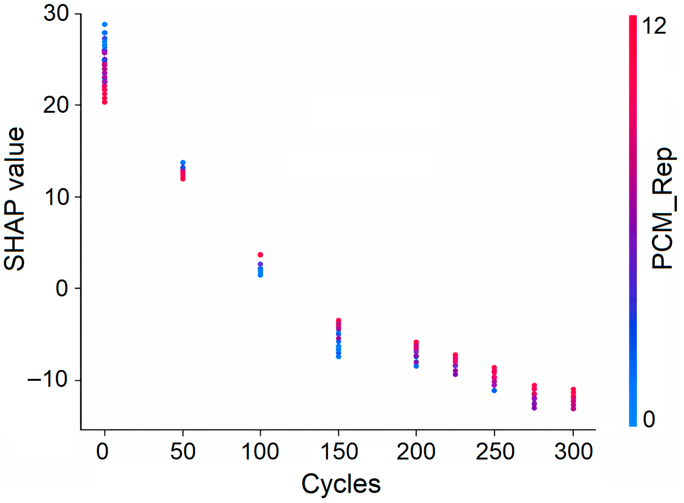
3.2.7. Dependence Plots: Interaction Between PCM and SF

Figure 7 shows a SHAP-dependent plot for the PCM substitution rate (PCM_Rep), with colours showing the volume proportion of steel fibres (SF_Vol). Dependence plots help to better understand how PCM and steel fibres interact. This plot shows directly how the marginal contribution of PCM to the anticipated RDEM changes with varied amounts of fibre.
There is a definite pattern of interaction: at a given PCM level, larger steel fibre content always leads to higher SHAP values, which shows that the positive contributions to durability are stronger. On the other hand, at low fibre contents, the extra benefit of PCM stays small. This shows that the efficiency of PCM is not independent; it is much affected by the presence of steel fibres.
In addition, the slope of the SHAP values in relation to PCM content is steeper as the fibre dose goes up. This means that the extra advantage of PCM is greater when there is enough mechanical reinforcement. This non-parallel distribution of coloured data points is clear proof of the interaction effects that the model found.

3.2.8. Synergistic Effects of PCM and Steel Fibres

This section presents results at two levels to distinctly differentiate between data-driven discoveries and physical interpretation. The synergistic effects between PCM and steel fibres are determined by experimental observations and SHAP analysis. Secondly, the observed patterns are analysed through recognised thermomechanical mechanisms of freeze–thaw damage in cementitious materials. SHAP analysis elucidates statistical correlations and interaction effects, whereas the suggested physical mechanisms offer a logical interpretation of these data rather than direct empirical evidence.
The SHAP analysis, combined with experimental observations, reveals a coherent mechanistic depiction of how PCM and steel fibres synergistically enhance freeze–thaw resistance. The SHAP dependence study also shows that the gap between different fibre levels is bigger when the PCM content goes up (Figure 7). This divergence reveals that the combined effect of PCM and steel fibres is not only additive; it shows a substantial coupling characteristic, which is consistent with the quantified interaction contribution (~46%) in the SHAP decomposition.
It is crucial to elucidate that SHAP analysis offers a data-driven interpretation of feature contributions inside the prediction model, rather than direct experimental validation of physical mechanisms. The found interaction patterns between PCM and steel fibres align with established thermomechanical behaviour; nonetheless, SHAP does not provide independent evidence of the underlying mechanisms. The proposed “thermal regulation—elastic buffering—fibre bridging” paradigm should be considered a physically plausible explanation, supported by both experimental evidence and insights derived from the model.

3.2.9. Thermal Regulation Mechanism (Latent Heat Effect)

The principal defensive mechanism of PCM microencapsulated is temperature regulation via latent heat storage and release. During the freezing process, the PCM core freezes into a solid, emitting latent heat as the temperature approaches the phase transition point. This exothermic process, by managing the internal temperature drop, creates a thermal shield that keeps the cementitious matrix from experiencing unanticipated temperature reductions.
The SHAP investigation confirms the importance of this mechanism; rising PCM doses consistently increase anticipated RDEM, and the effect is more pronounced with increasing PCM contents, as demonstrated by positive SHAP values of PCM_Rep. This has two key benefits for thermal buffering:
First, PCM minimises the temperature differential between the inside and outside of the concrete by slowing the rate of change in temperature. Even without total freezing, differential strains resulting from strong heat gradients can cause microcracking. As a result, PCM’s regulating effect reduces heat-related stress.
Second, PCM minimises the number of effective freeze–thaw cycles that the interior structure experiences by delaying the beginning of freezing in the pore system. Despite exterior temperatures ranging from −18 °C to +5 °C, PCM regions can see fewer true freeze incidents, extending service life.
The experimental results support this conclusion, showing that under identical external exposure conditions, mixtures containing 12% PCM maintained a substantially higher RDEM after 300 cycles (72.6%) compared to the reference mixture (61.2%). This 11.4% increase can be directly attributed to the temperature-regulating effects of the PCM.

3.2.10. Elastic Buffering of Microcapsule Shells

In addition to latent heat effects, the mechanical qualities of the microcapsule’s shell contribute to frost resistance. The elastic structure of the polymer shell (melamine-formaldehyde resin) allows it to stretch under pressure without tearing. The hydraulic pressure generated by the volumetric expansion (about 9%) of ice within capillary pores has the potential to break the hard cement matrix. Nonetheless, this pressure can induce the elastic shell of a microcapsule to deform, absorbing energy and reducing stress.
This flexible buffering technique is most successful at high PCM concentrations (912%), which are sufficient to produce an infiltrating network of microcapsules in the matrix. At such concentrations, the elastic shells form a dispersed energy-absorbing structure capable of sustaining ice expansion without causing damage to the surrounding cement paste [19]. This clarification is validated by the SHAP study, which shows its interaction with steel fibres. If the PCM relied solely on thermal management, it would be able to accumulate its benefits regardless of fibre composition. The enhanced effect of PCM in fibre-reinforced mixtures is believed to result from a mechanical contribution. Elastic buffering of the microcapsules reduces the force needed to initiate microscale cracks, thereby easing the stress on the fibres and improving their bridging performance. Although soft inclusions might be expected to weaken matrix integrity, the combined two-step process of thermo-regulation and elastic buffering explains why higher PCM dosages (12%) in conjunction with steel fibres lead to improved performance. Flexible microcapsules are not defects, but rather scattered stress absorbers that protect the rigid cement framework.

3.2.11. Fibre Bridging and Crack Restraint

Steel fibres provide the primary mechanical protection against freeze–thaw degradation by redistributing stress and bridging cracks [3]. Increased fibre levels have a beneficial effect on predicted lifetime on a periodic basis, and SHAP analysis shows that SF_Vol is the second most significant attribute.
The reinforcing mechanism operates at many scales. Individual fibres bridge incipient cracks at the microscale level, transmitting tensile loads across the crack face and preventing crack opening. This fracture-bridging action prevents isolated microcracks from cracking together (posing a hazard to structural integrity). The fibre network is a three-dimensional structure that forms a strong skeleton on the macroscopic level, keeping the cement structure stiff as it splits [30]. The experimental RDEM statistics indicate this effect: after 300 cycles, mixes containing 1.2% SF still had 74.3% of RDEM, while the reference (1.2%) had 61.2 percent, which is directly proportional to fibre reinforcement.
The time required for fibres to become effective is a key distinguishing characteristic. In the highly degraded phase (i.e., the phase at which crack networks would otherwise propagate catastrophically), the fibres appear to be quite helpful, as the SHAP dependency graphs reveal that SF_Vol contributions become increasingly positive at even higher cycle numbers. This is consistent with the physical knowledge that fibres do not prevent fracture formation, but rather govern its progression once formed [7]. Fibre bridging begins to operate only when matrix cracking has occurred.

3.2.12. Quantification of ThermoMechanical Coupling

The SHAP interaction study allows for a quantitative examination of the thermomechanical relationship between PCM and steel fibres. The synergistic contribution can be calculated and assessed by breaking down the prediction into main effects and interaction effects. In the case of an extreme-performance configuration (12% PCM + 1.2%SF), the total SHAP in predicting RDEM is somewhat greater than +5.2 compared to the baseline (average prediction). In this total, approximately 2.8 (54) is due to the significant effects of PCM and SF individually, while 2.4 (46) is due to the interaction effect—the additional benefit above and above simple additivity. This is practically a balanced distribution of the primary and interaction effects, demonstrating quantitatively the coupled configurations’ excellent performance as a result of synergy rather than superposition.
The economic model’s overall SHAP contribution (9% PCM + 0.9% SF) is approximately +3.8, with the main effects being the highest (2.2 or 58%), followed by the interaction effects (1.6 or 42%). The percentage contribution is large, despite the fact that absolute synergy is decreased at such moderate dosages, demonstrating that synergistic advantages are not limited to severe formulations.
A physical explanation for this quantitative synergy is straightforward: PCM reduces stress on the fibre reinforcement system through elastic buffering and temperature regulation. PCM will lessen the displacements necessary for fibres to cross the crack by minimising temperature differences and absorbing frost expansion pressures. Fibres, on the other hand, provide the structural support essential to keep the matrix together while allowing PCM to work in recurrent cycles [41]. This mutual reinforcement creates a positive feedback loop that benefits both materials, with PCM insulating the matrix to allow fibres to bridge and fibres insulating the matrix to allow PCM to regulate.
The thermomechanical contacting mechanism revealed by SHAP analysis calls into question the traditional idea that all functional additives invariably cause unfavourable interfacial defects and so reduce durability. Instead, the employment of appropriately engineered PCM and steel fibres results in a composite system in which the whole is substantially greater than the sum of its parts. The findings of this study have important significance for building high-durability concrete to be used in hostile locations.
It is important to emphasise that the quantified interaction effects derived from SHAP represent statistical contributions within the predictive model. While these results provide strong evidence of synergy between PCM and steel fibres, the underlying physical mechanisms are inferred based on established material behaviour rather than directly measured in this study. Therefore, the proposed thermomechanical coupling mechanism should be understood as a physically consistent interpretation of the data-driven findings.


4. Discussion

4.1. Interpretation of the ThermoMechanical Synergistic Mechanism

The mechanistic interpretations in this section are based on a synthesis of experimental observations and SHAP-based data analysis. It is important to acknowledge that, while SHAP offers significant insights into feature interactions and relative relevance, it does not independently validate physical mechanisms. The SHAP analysis combined with experimental observations reveals a coherent mechanistic framework for understanding how PCM and steel fibres synergistically enhance freeze–thaw resistance. This section interprets these findings in the context of established frost damage theory and materials science principles.
The synergistic effect of PCM and steel fibres can be explained as a linked thermomechanical interaction rather than a simple additive contribution [50]. PCM largely lowers internal stress buildup by regulating temperature gradients and delaying ice formation inside the pore structure. This causes a decrease in hydraulic and osmotic pressures during freeze–thaw cycles.
Steel fibres, on the other hand, help to maintain mechanical stability by bridging microcracks and improving stress transfer across damaged regions. The presence of fibres raises the energy required for fracture propagation and slows the transition from microcracking to macrocrack coalescence [19].
The SHAP study reflects the interaction of these two mechanisms, with PCM and steel fibres contributing more than the total of their individual impacts. This demonstrates a non-linear coupling behaviour in which thermal stress reduction supplied by PCM improves fibre bridging effectiveness, while the fibres preserve structural integrity in the presence of PCM-induced microstructural weakening.

4.1.1. PCM as Thermal Shield and Flexible Buffer

According to the experimental data and SHAP analysis, heat regulation and elastic buffering are two additional processes of microencapsulated PCM that improve frost resistance.
(1)
Thermal Shield Mechanism: During freezing, the paraffin core of the microcapsules transitions from a liquid to a solid state, and the latent heat (about 180,200 J/g) is released as the ambient temperature drops below 0 °C. This exothermic process is used to limit the internal temperature drop of the concrete and maintain a steady temperature, resulting in a form of thermal shield that protects the cementitious matrix from extreme temperature changes [35,36]. The value of the given process is supported by the SHAP analysis. PCM_Rep invariably has a beneficial impact on anticipated RDEM, and the effect is stronger as PCM content increases (Figure 4). This thermal buffering has two benefits. To begin, PCM minimises the thermal gradient between the concrete surface and the inside by slowing the pace at which temperatures fluctuate. Even when there is no total freezing, different sharp heat gradients cause lateral strains that can lead to microcracking [37]. Second, PCM limits the effectiveness of freeze–thaw cycles in the inner structure by delaying the onset of freezing in the pore system. Although the ambient temperature varies between −18 and +5 degrees Celsius, areas with PCM can see fewer true freeze cycles, enhancing service life [38].
(2)
Flexible Buffer Mechanism: The mechanical features of the microcapsule shell contribute to frost resistance beyond that caused by latent heat. Because of its natural elasticity (elastic modulus of approximately 35 GPa), the polymer shell (melamine-formaldehyde resin) can bend under pressure without breaking [39]. When ice accumulates in capillary pores, the volumetric expansion (about 9%) causes hydraulic pressure and has the ability to shatter the stiff cement matrix. However, the elastic shell of a microcapsule can flex under this pressure, absorbing energy and reducing stress [40]. This so-called flexible buffering process works best at high PCM doses (9–12%) and when the microcapsules are dense enough to form a scattered energy-absorbing network in the matrix. At these concentrations, the elastic shells form a percolating structure that can withstand cold expansion without causing damage to the surrounding cement paste [41]. The amplification of the PCM effect in fibre-reinforced composites (Figure 5) means that elastic buffering improves fibre bridging by absorbing stresses at the micro level, hence reducing the crack-opening force that fibres must suffer. The SHAP interaction study supports this conclusion.
Although soft inclusions are typically assumed to weaken the matrix, the two-step process of thermoregulation and elastic buffering enables the use of high PCM concentrations (12%), resulting in enhanced performance [18,19]. Instead of functioning as vices, the flexible microcapsules function as scattered stress absorbers, protecting the hard cement framework. This discovery challenges the established principle that “specialised multiphase composites inevitably result in deterioration of durability,” and so offers up new opportunities for developing high-performance concrete with helpful inclusions.
Even though PCM has been shown to improve freeze–thaw resistance, it is crucial to recognise that it may have negative impacts on mechanical properties. Increased porosity, weakened interfacial transition zones (ITZ), and decreased compressive and flexural strength can result from the addition of microencapsulated PCM, which replaces a portion of the fine aggregate. These effects are a significant barrier to the structural applications of PCM-modified concrete and have been extensively documented in earlier research.
Steel fibres, which offer mechanical reinforcement by bridging microcracks and preserving load-transfer capacity [17], are used in the current work to lessen this potential disadvantage. The SHAP study also shows that, especially at increasing PCM levels, steel fibres are crucial for maintaining structural integrity. Consequently, the enhanced durability seen in PCM–steel fibre composites should be seen as the outcome of a balanced design approach in which the mechanical reinforcing of fibres complements the thermal advantages of PCM. This emphasises how crucial it is to take mechanical performance and durability enhancement into account when designing practical mixes.

4.1.2. Steel Fibres as Primary Mechanical Defence

The main mechanical protection against freeze–thaw degradation in steel is provided by stress redistribution and fibre crack-bridging. Every increase in fibre content contributes positively to predicted durability, and the SHAP analysis reveals that SF_Vol is the second most significant attribute (Figure 3). The reinforcing mechanism works at various scales. Individual fibre bridging over incipient cracks occurs at the microscale, where tension stresses are transmitted across the crack face, preventing crack opening [42]. This crack-bridging action prevents isolated microcracks from merging into interconnected crack networks that could compromise structural integrity [43]. The copper coating strengthens the fibre–matrix interaction even in the presence of many freeze–thaw cycles, ensuring high stress transmission [44].
The three-dimensional fibre network serves as a macro-scale skeleton reinforcing framework, keeping the cement structure solid as it deteriorates. The experimental RDEM statistics can explain this: mixtures with 1.2% SF had 74.3% of the original RDEM, while the reference mix had 61.2%—a 13.1 percentage-point difference that was definitely related to fibre reinforcement. Fibres play a particularly crucial role in the later stages of deterioration, where crack networks would otherwise propagate extensively. SHAP dependency plots indicate that the contribution of SF_VOL becomes increasingly positive as the number of cycles increases. This is consistent with the physical assumption that fibres do not restrict the production of cracks, as they would grow on their own, but rather control their spread once created [45]. Fibre bridging is initiated only when the matrix cracks.

4.1.3. Coupled Enhancement Under F300 Loading

This study’s most significant innovation is that the thermomechanical interaction between PCM and steel fibre under F300 loading conditions is quantitatively confirmed. According to the SHAP interaction analysis (Section 3.2.6), the cumulative effect is significantly larger than the sum of individual contributions.
Approximately 46% of the SHAP contribution of the RDEM prediction to the extreme-performance configuration (12% PCM + 1.2% SF) is due to interaction effects rather than main effects. This nearly equal separation is measurable in nature, demonstrating that the magnificent outcome of connected systems is the result of synergy rather than superposition. Mutual reinforcement between the two defence mechanisms might be viewed as the physical foundation of this synergy.
PCM reduces the tensile stress that fibres must endure. By moderating temperature gradients and alleviating some of the frost-induced expansion pressures, PCM limits crack-opening movements, effectively buffering the fibres with its flexibility. Smaller fracture widths in bridge fibres reduce tensile stress, lowering the danger of fibre withdrawal or rupture [46]. This protective action helps fibres to withstand longer freeze–thaw cycles. The cementitious matrix is physically continuous with steel fibres to prevent the formation of large cracks that restrict heat transfer channels and jeopardise PCM’s ability to manage its temperature. It is also possible to effectively disseminate latent heat in the concrete mass because the continuous matrix ensures that microcapsules are entrenched in the continuous media [48].
Under F300 loading, where the combined effects of intense thermal cycling and accumulated mechanical damage would typically overwhelm any single protective measure, this synergistic enhancement becomes particularly significant. The safety margin is quite low because the reference combination (0% PCM, 0% SF) only passes the F300 standards (RDEM = 61.2% and 300 cycles). Conversely, after 300 cycles, the extreme-performance design achieves RDEM = 72.6%, indicating significant levels of durability redundancy, which is required for safety-critical infrastructure.

4.2. Implications for Mix Design Optimisation

The integration of high-accuracy prediction and mechanistic interpretability enables a rational approach to mix design optimisation that balances performance, cost, and constructability.

4.2.1. Lifecycle Frost-Resistance Risk Evolution

Figure 7 illustrates that the contribution of freeze–thaw cycles gradually grows to negative values as the cycle advances, implying that stiffness degrades more quickly when environmental loading is cumulative. Nonetheless, greater PCM replacement levels mitigate this negative effect, particularly during later freeze–thaw episodes. This demonstrates that high-content PCM has significant protective benefits on long-term durability performance. The integrated thermomechanical system, in conjunction with enough steel fibre reinforcing, effectively eliminates the possibility of frost resistance throughout the life cycle.

4.2.2. Determination of Dosage Critical Thresholds

Figure 6 shows that the relationship between observed RDEM and PCM_Rep SHAP dependence plot is not linear. The steeper slope is in the 6% range, the moderate one is in the 6–9% region, and the plateau is at 9% or higher. Previous research has revealed that an optimal PCM concentration is 5 to 10% to achieve balanced performance [41,44]. The trend indicates that PCM doses are experiencing a 9% decline in marginal gains.
The steel fibre content SHAP analysis indicates a linear connection up to 1.2, indicating that the benefits of the fibre continue to improve as the range is measured. Nonetheless, the upper limit of 1.25% in the fibre form and mixing equipment used in this investigation appears fair in terms of cost, workability, and probable fibre balling during high dosages [5]. The greatest interaction effect between PCM and SF is reported in the ranges of 6–12% PCM and 0.6–1.2% SF. SF suggests that moderate-to-high doses of both compounds maximise synergistic benefits.
It should also be noted that, while excessive PCM content is advantageous for heat control, it could reduce mechanical strength and stiffness by introducing low-modulus inclusions and increasing porosity. As a result, choosing the appropriate PCM dosage must take into account both durability performance and structural requirements. The identified ideal range (about 9–12%) strikes a balance between enhancing freeze–thaw resistance and minimising mechanical degradation, especially when combined with appropriate steel fibre reinforcing.

4.2.3. Cost-Effective Configuration (9% PCM + 0.9% SF)

In the examination of the lifetime risk evolution and dosage threshold, it is clear that the 9% PCM and 0.9% steel fibre configuration is the best performance–cost balance for typical severe cold-region airports. This configuration meets the F300 durability limits of MH/T 5004-2024, with an anticipated RDEM of 79.4% at 200 cycles and 66.8% at 300 cycles, 6.8 percentage points more than the 60% minimum. The mass loss after 300 cycles was found to be 1.95, which is significantly lower than the 5% specification limit. Economically, this setup retains the requisite PCM content to activate both heat regulation and elastic buffering processes while avoiding the diminishing returns associated with PCM dosages greater than 9%. The percentage of steel fibre (0.9) provides excellent crack-bridging reinforcement without the issue of workability or the increased costs associated with adopting a greater fibre dose.
Workability is another issue that contributes to this decision. The superplasticiser dosage (25.8 kg/m3) remained tolerable at 9% PCM + 0.9% SF, with a Vebe consistency ranging from 10 to 15 s. An increase in PCM dosage necessitates the addition of extra superplasticiser (40.8 kg/m3 of 12% PCM), which raises the material’s cost and may impact early-age characteristics and setting time [23].
As such, the recommended solution of most extreme cold-region airports can be considered a promising mix design configuration under the controlled experimental conditions of this study. It demonstrates a favourable balance between durability performance and material efficiency; however, its applicability to real airport pavements requires further validation under field conditions.

4.2.4. Extreme-Performance Configuration (12% PCM + 1.2% SF)

The design objective shifts to achieve the greatest freeze–thaw resistance and durability redundancy for airports located in ultra-cold environments, where minimum monthly temperatures are below −10 °C, where freeze–thaw cycles occur more than 300 times per year, or where de-icing chemicals are extensively used. The 12% PCM + 1.2% SF scenario accounts for high exposure circumstances. This design allows the thermomechanical coupling mechanism to fully engage after 300 cycles, with an estimated RDEM of 72.6, which is 5.8 percentage points greater than the economical arrangement and 11.4 percentage points higher than the reference.
Aside from increasing the latent heat storage capacity, the higher PCM dose (12) creates a thick network of microcapsules that provides a significant amount of elastic buffering against hydraulic pressure caused by frost. At the same time, the 1.2% volume percentage of steel fibres creates a robust three-dimensional fracture-bridging skeleton that improves crack restraint and stiffness preservation. According to the SHAP analysis, their interaction effect is the biggest, with roughly 46% of the overall benefit resulting from synergy rather than additive effects. In circumstances when durability redundancy is critical, this significant synergy will justify the material’s increased cost.
This high-performance configuration may be considered a potential candidate for applications in extremely cold regions or high-risk zones, based on its superior freeze–thaw resistance observed under laboratory conditions. However, its practical implementation should be further evaluated considering additional factors such as de-icing salt exposure, fatigue loading, surface wear, and environmental variability.
Because of the high PCM content, the arrangement also offers increased active snow-melting capacity, which may lessen the need for de-icing chemicals and the related environmental effects—an extra advantage for environmentally sensitive places.

4.2.5. Statistical Distribution Analysis of Durability Indicators

To investigate the variability and statistical stability of the freeze–thaw durability indicators, mass loss and relative dynamic modulus were plotted in violin-box plots with varying PCM replacement rates and steel fibre volume fractions (Figure 8, Figure 9, Figure 10 and Figure 11). Unlike traditional mean-value comparisons, violin-box plots provide a more detailed representation of data dispersion by displaying the probability density distribution alongside significant statistical parameters such as the median, quartiles, and outliers.
Figure 8 and Figure 9 show the distribution of mass loss and RDEM for different PCM compositions. Durability indices are becoming more concentrated as the PCM substitution rate increases, indicating a decrease in freeze–thaw damage variance. This observation validates PCM’s thermal buffering function, which reduces frost-induced strains and aids in internal temperature gradients. The distribution likewise narrows at higher PCM levels, showing that the concrete matrix is more resilient to repeated freeze–thaw loads.
Figure 10 and Figure 11 show statistical distributions of mixes, including different volume fractions of steel fibre. As the fibre content increases, there is a discernible growing trend in the RDEM distribution, as well as a decrease in the dispersion of mass loss values. Such activity might be interpreted as steel fibres’ ability to fill cracks, prevent the spread of microcracks, and maintain their internal load-transfer structure.
Violet-box plot analysis lends confirmation to the thermomechanical synergy between PCM and steel fibres discovered through SHAP interpretation. Aside from increased average life, the optimised formulations exhibit greater statistical stability, which is a fundamental need for reliable operation in airport pavement systems subjected to harsh freeze–thaw conditions.
Violin-box plots were used in distribution-based analyses to further assess the statistical significance and variability of the experimental outcomes. These plots offer a thorough depiction of data dispersion, probability density, and quartile distribution, in contrast to mean-value comparisons, allowing for a more exacting evaluation of result consistency and dependability.
In general, the relatively narrow distributions and lack of significant outliers suggest that the gains in freeze–thaw performance are both large and statistically consistent among replicate samples. This increases the trustworthiness of the experimental results and strengthens the validity of the subsequent machine learning modelling.

4.3. Practical Implementation for Airport Pavements

4.3.1. Digital Transformation of F300 Durability Verification

The suggested paradigm, which replaces almost instant predictive analysis with a traditionally protracted laboratory test, represents a significant departure in the durability assessment technique. The three months of sequential testing of conventional F300 testing, which includes seven days of specimen preparation, twenty-eight days of curing, four days of saturation, and 80–100 days of freeze–thaw cycling, is a major bottleneck in mix design optimisation, especially for emergency rehabilitation and fast-track projects. This assessment schedule is reduced from several months to milliseconds by using an XGBoost-based model, which can forecast mass loss and relative dynamic modulus of elasticity with greater than 99% accuracy using only the mix design parameters, steel fibre content, and PCM content. Designers can quickly test dozens of alternative mix proportions in a few seconds to determine the optimal blends before committing to laboratory verification. To encourage educated trade-off judgements, it also enables fast sensitivity analysis, with the impact of PCM or fibre content changes analysed instantaneously. Even during construction, the framework allows for real-time adjustment: if material characteristics do not meet criteria, the influence on long-term durability may be evaluated instantly. This digital transition will also accelerate the design discovery process, decreasing overall project durations by weeks or months. However, physical testing of the final designs is still necessary.
It is vital to emphasise that the suggested machine learning architecture is not meant to take the place of the usual freeze–thaw testing methods that are required by engineering regulations. Instead, it is an extra tool for quickly screening and testing mix concepts in a controlled setting. The model is based on a stable cementitious system, a constant water-binder ratio, and certain boundary conditions. This makes it hard to use it directly with other types of materials. So, standardised laboratory testing is still needed for final validation to make sure that engineering and safety criteria are met.

4.3.2. Integration with Existing Design Standards

A critical requirement for practical adoption is compatibility with existing regulatory frameworks. The proposed framework has been specifically developed to align with Chinese civil aviation standards:
  • MH/T 5004-2024 (Design Specification): The framework is specifically aimed at the F300 durability requirement of the Category 4 airport pavement. The predictions are set to the 300-cycle endpoint, and RDEM must be 60% or higher with a mass loss of 5% or less as stipulated in the standard.
  • MH/T 5006-2024 (Construction Specification): The slip-form paving construction requirements are based on the workability control strategy (Vebe consistency of 10 to 15 s through superplasticiser modification), which is required to make the recommended mixtures meet the construction requirements.
  • GB/T 50082-2009 (Test Method): The experimental database was prepared based on the standard rapid freezing and thawing procedure identified in this national standard, such that predictions can be directly compared to the traditional test outcomes.
The framework can be extended to other regulatory contexts by retraining on databases generated according to relevant standards (e.g., ASTM C666 [51] for international applications). The methodology itself is standard-agnostic; only the training data must reflect the relevant testing protocols.

4.3.3. Construction Workability Considerations

Successful implementation of high-performance concrete requires attention to fresh-state properties. The experimental programme demonstrated that both PCM and steel fibres affect workability, but through different mechanisms:
(a)
PCM enhances the amount of water needed because the specific surface area of the microcapsules is very high and hence captures the mixing water as well as decreases the effective free water content. This was effectively overcome by the variation in the dosage of superplasticiser; the dosage of superplasticiser was increased to 40.8 kg/m3 (12% PCM) at constant workability, which required the dosage to be 10.8 kg/m3 (0% PCM) to maintain the same workability.
(b)
Physical interference and augmented interior friction occur in steel fibres and influence workability. The percentage fibre content of 1.2% required a close dispersion of the fibres during the mixing process to prevent fibre balling. The suggested mixing (customised gradual addition of fibres with prolonged wet mixing) was successful with all mixtures.
(c)
PCM content and dosage of SP required (average 2.5 kg/m3 extra SP per 1% increase in PCM) offers a basis upon which trial batching can commence.
(d)
Dry incorporation of all solids other than fibres (120 s), gradual incorporation of fibres (60 s), incorporation of PCM, followed by addition of water and SP incorporation with longer mixing (180 s) is a requirement in order to achieve uniform dispersion.
(e)
Each batch should be checked in terms of Vebe consistency, and SP should be regulated, according to the requirements, in order to stay within the target range.
(f)
PCM content is to be checked after a period of time, as it is possible that agglomeration or segregation can change workability and hardening properties.
It is important to note that the experimental programme in this study is only about how well data can handle freezing and thawing in a controlled laboratory setting. In actual airport pavement conditions, durability is affected by several interconnected elements, including de-icing salt corrosion, recurrent aeroplane loading (fatigue), surface wear, and changes in the environment. The current study did not directly address these consequences. Consequently, although the suggested mix designs exhibit robust freeze–thaw behaviour, their immediate implementation in field circumstances necessitates prudence, and additional validation through extensive durability testing and field trials is advisable.

4.4. Applicability Domain and Model Limitations

The suggested XGBoost model shows good prediction accuracy and robustness in the dataset that was analysed. However, the range of input variables that were utilised to build the model limits its usefulness. The training data were produced in controlled experimental settings with defined parameter ranges, including a PCM replacement rate of 0–12%, a steel fibre volume percentage of 0–1.2%, and freeze–thaw cycles ranging from 0 to 300. Because of this, the model’s forecasts can only be trusted in these ranges.
Extrapolation beyond these limits, including using higher PCM amounts, different fibre types or doses, or longer freeze–thaw exposure times, could make predictions less accurate because there is not enough relevant training data. This restriction is prevalent in data-driven models, especially when they are constructed from relatively small yet high-quality experimental datasets.
Also, the boundary-controlled dataset makes the internal consistency and signal-to-noise ratio better, but it might make it harder for the model to pick up on changes in real-world conditions, like changes in the sources of raw materials, changes in the environment, or changes in construction practices.
Another key limitation has to do with how the data is split up. Because the dataset has several measurements of the same mix proportions taken at different freeze–thaw cycles, dividing it up randomly could cause correlations between the training and testing sets. This can make the predicted performance seem better than it really is, since the model might only learn patterns that are specific to the mix instead of relationships that can be used in other situations.
A more stringent validation methodology for further research would entail group-based partitioning, wherein all data from a specified mix proportion are allocated only to either the training or testing set. This would give a better idea of how well the model can apply to mix designs that it has never seen before. Adding more independent mix compositions to the dataset would make the model even more robust and able to generalise.
Future research should concentrate on augmenting the dataset to encompass a broader spectrum of material compositions, ambient circumstances, and field validation data. Adding datasets from several sources and other factors that can affect the model (such as air content, curing variances, or salt exposure) would make it even better at generalising and being useful in a wider range of engineering situations.

5. Conclusions

This research developed an XGBoost-based framework to address challenges in cold-region airport pavement construction using a high-fidelity small-sample database. The main conclusions of the study are summarised as follows:
  • The XGBoost-based framework confirmed outstanding predictive accuracy for freeze–thaw durability. It predicted mass loss (R2 = 0.9938, RMSE = 0.0957) and relative dynamic modulus (RDEM) (R2 = 0.9935, RMSE = 0.9687) under F300 cycles. The model reduces durability evaluation time from several months of laboratory testing to milliseconds. This approach enables rapid mix design and real-time durability assessment for cold-region airport pavements.
  • SHAP analysis revealed a clear thermomechanical coupling mechanism between steel fibres (SF) and phase-change materials (PCM). These materials work together to enhance crack bridging and improve freeze–thaw resistance. This finding provides a new strategy for designing high-performance multi-phase composite concrete.
  • Two mix design configurations demonstrated excellent freeze–thaw performance under laboratory conditions and may serve as reference solutions for further engineering evaluation. The cost-effective configuration (9% PCM + 0.9% SF) achieved 66.8% RDEM after 300 cycles with a 6.8% safety margin. These designs balance durability, economic feasibility, and structural performance.
  • The findings suggest that optimal performance is not achieved by maximising individual components, but by coordinating their combined effects. The identified mix configurations demonstrate that durability improvements can be achieved while maintaining practical considerations such as workability and material efficiency.
The proposed framework supports digital decision-making for airport pavement construction and aligns with MH/T 5004-2024 and MH/T 5006-2024 standards. SHAP-based interpretability improves confidence in AI-assisted engineering decisions. Future studies should expand the dataset with more material variables, conduct long-term field validation, and extend the framework to predict additional durability indicators such as fatigue life, salt scaling resistance, and chloride penetration.

Author Contributions

H.L.: methodology, formal analysis, funding acquisition, visualisation, and validation. M.S.: project administration, editing, funding acquisition, data curation, and validation. Y.W.: writing, investigation, and visualisation. C.L.: writing, draft preparation, conceptualisation, software, and resources. All authors have read and agreed to the published version of the manuscript.

Funding

This work was conducted with support from the China–Central and Eastern European Countries Joint Education Program (2021111), the Key Research and Development Program of Liaoning Province, China (2024JH2/10210006), the Research and Development Project of Large Enterprises (2024020700249), and the Fundamental Research Funds for the Central Universities (S20250075, D20250052, D20240080).

Data Availability Statement

The original contributions presented in this study are included in the article. Further inquiries can be directed to the corresponding author.

Conflicts of Interest

The authors declare no conflicts of interest.

Appendix A. Detailed Material Properties

Table A1. Chemical Composition and Physical Properties of Cementitious Materials.
PropertyCement (P·C 42.5)Fly Ash (Class F)Silica Fume
Chemical Composition (%)
SiO221.352.494.2
Al2O35.228.60.8
Fe2O33.86.20.5
CaO62.14.80.3
MgO2.41.20.6
SO32.10.30.2
Loss on ignition2.33.52.1
Physical Properties
Specific gravity3.152.322.20
Specific surface area (m2/kg)36541018,500
Mean particle size (μm)18120.15
Table A2. Physical Properties of Aggregates.
PropertyCoarse AggregateFine Aggregate
Maximum nominal size (mm)204.75
Specific gravity (SSD)2.682.62
Water absorption (%)0.81.2
Fineness modulus2.7
Bulk density (kg/m3)15201610
Void content (%)4238
Crushing value (%)18
Table A3. Properties of Microencapsulated Phase-Change Material (mPCM).
PropertyValue
Core materialParaffin wax
Shell materialMelamine-formaldehyde resin
Phase transition temperature (°C)0.5 (freezing), 2.1 (melting)
Latent heat capacity (J/g)185 ± 8
Mean particle size (μm)22.5
Shell thickness (μm)2.5
Specific gravity0.92
Thermal conductivity (W/m·K)0.18
Elastic modulus of shell (GPa)3.8
Decomposition temperature (°C)>200
Table A4. Properties of Steel Fibres.
PropertyValue
Fibre typeStraight, copper-coated
Length (mm)13
Diameter (mm)0.20
Aspect ratio (L/D)65
Tensile strength (MPa)≥2000
Elastic modulus (GPa)200
Specific gravity7.85
Copper coating thickness (μm)5
Number of fibres per kgApproximately 14,500
Table A5. Properties of Superplasticiser.
PropertyValue
TypePolycarboxylate-based
Solid content (%)40
Specific gravity1.08
pH value6.5
Water reduction rate (%)>30
Recommended dosage range (% of binder)0.8–2.5

Appendix B. Complete Mix Proportions

Table A6. Full Factorial Experimental Design Matrix.
Mix No.Group CodePCM (%)SF (%)Cement (kg/m3)Fly Ash (kg/m3)Silica Fume (kg/m3)Water (kg/m3)Coarse Aggregate (kg/m3)Fine Aggregate (kg/m3)PCM Mass (kg/m3)SF Mass (kg/m3)SP (kg/m3)
1PCM0-SF000.0322.586.021.5124.71148.1645.00.00.010.8
2PCM0-SF0.600.6322.586.021.5124.71148.1645.00.047.110.8
3PCM0-SF0.900.9322.586.021.5124.71148.1645.00.070.710.8
4PCM0-SF1.201.2322.586.021.5124.71148.1645.00.094.210.8
5PCM3-SF030.0322.586.021.5124.71148.1625.719.40.012.5
6PCM3-SF0.630.6322.586.021.5124.71148.1625.719.447.112.5
7PCM3-SF0.930.9322.586.021.5124.71148.1625.719.470.712.5
8PCM3-SF1.231.2322.586.021.5124.71148.1625.719.494.212.5
9PCM6-SF060.0322.586.021.5124.71148.1606.338.70.015.8
10PCM6-SF0.660.6322.586.021.5124.71148.1606.338.747.115.8
11PCM6-SF0.960.9322.586.021.5124.71148.1606.338.770.715.8
12PCM6-SF1.261.2322.586.021.5124.71148.1606.338.794.215.8
13PCM9-SF090.0322.586.021.5124.71148.1587.058.10.025.8
14PCM9-SF0.690.6322.586.021.5124.71148.1587.058.147.125.8
15PCM9-SF0.990.9322.586.021.5124.71148.1587.058.170.725.8
16PCM9-SF1.291.2322.586.021.5124.71148.1587.058.194.225.8
17PCM12-SF0120.0322.586.021.5124.71148.1567.677.40.040.8
18PCM12-SF0.6120.6322.586.021.5124.71148.1567.677.447.140.8
19PCM12-SF0.9120.9322.586.021.5124.71148.1567.677.470.740.8
20PCM12-SF1.2121.2322.586.021.5124.71148.1567.677.494.240.8
Notes: All mixtures have a constant water-to-binder ratio (w/b) = 0.29. Total binder content = 430 kg/m3 (cement + fly ash + silica fume). Superplasticiser (SP) dosage adjusted to maintain a Vebe consistency of 10–15 s.

Appendix C. Complete Experimental Dataset

Table A7. Full Freeze–Thaw Durability Dataset (145 Samples).
Sample IDMix No.PCM (%)SF (%)CyclesMass Loss (%)RDEM (%)
R1-0100.000.00100.0
R1-50100.0500.4294.6
R1-100100.01000.9887.3
R1-150100.01501.5678.5
R1-200100.02001.9870.2
R1-250100.02502.2364.8
R1-300100.03002.4561.2
R2-0200.600.00100.0
R2-50200.6500.3895.2
R2-100200.61000.8489.4
R2-150200.61501.3282.6
R2-200200.62001.7176.3
R2-250200.62501.9871.2
R2-300200.63002.1867.5
R3-0300.900.00100.0
R3-50300.9500.3595.8
R3-100300.91000.7890.5
R3-150300.91501.2184.7
R3-200300.92001.5879.2
R3-250300.92501.8474.6
R3-300300.93002.0471.3
R4-0401.200.00100.0
R4-50401.2500.3296.4
R4-100401.21000.7191.8
R4-150401.21501.1286.5
R4-200401.22001.4881.4
R4-250401.22501.7577.2
R4-300401.23001.9874.3
R5-0530.000.00100.0
R5-50530.0500.4195.0
R5-100530.01000.9488.5
R5-150530.01501.4880.8
R5-200530.02001.9273.6
R5-250530.02502.1868.2
R5-300530.03002.3864.8
R6-0630.600.00100.0
R6-50630.6500.3795.6
R6-100630.61000.8190.2
R6-150630.61501.2684.0
R6-200630.62001.6478.2
R6-250630.62501.9273.4
R6-300630.63002.1269.8
R7-0730.900.00100.0
R7-50730.9500.3496.2
R7-100730.91000.7591.4
R7-150730.91501.1685.8
R7-200730.92001.5280.5
R7-250730.92501.7976.1
R7-300730.93002.0172.8
R8-0831.200.00100.0
R8-50831.2500.3196.8
R8-100831.21000.6892.5
R8-150831.21501.0687.6
R8-200831.22001.4182.8
R8-250831.22501.6878.6
R8-300831.23001.9275.4
R9-0960.000.00100.0
R9-50960.0500.3995.4
R9-100960.01000.8989.2
R9-150960.01501.4182.4
R9-200960.02001.8475.8
R9-250960.02502.1270.6
R9-300960.03002.3266.9
R10-01060.600.00100.0
R10-501060.6500.3596.0
R10-1001060.61000.7791.0
R10-1501060.61501.1985.4
R10-2001060.62001.5680.0
R10-2501060.62501.8475.4
R10-3001060.63002.0571.9
R11-01160.900.00100.0
R11-501160.9500.3296.5
R11-1001160.91000.7192.2
R11-1501160.91501.1087.2
R11-2001160.92001.4582.4
R11-2501160.92501.7278.2
R11-3001160.93001.9574.8
R12-01261.200.00100.0
R12-501261.2500.2997.0
R12-1001261.21000.6493.2
R12-1501261.21501.0188.6
R12-2001261.22001.3484.2
R12-2501261.22501.6080.4
R12-3001261.23001.8377.2
R13-01390.000.00100.0
R13-501390.0500.3895.8
R13-1001390.01000.8490.2
R13-1501390.01501.3384.0
R13-2001390.02001.7477.8
R13-2501390.02502.0172.8
R13-3001390.03002.2269.2
R14-01490.600.00100.0
R14-501490.6500.3496.4
R14-1001490.61000.7491.8
R14-1501490.61501.1686.6
R14-2001490.62001.5181.4
R14-2501490.62501.7877.0
R14-3001490.63001.9973.5
R15-01590.900.00100.0
R15-501590.9500.3196.9
R15-1001590.91000.6792.8
R15-1501590.91501.0588.0
R15-2001590.92001.3883.4
R15-2501590.92501.6479.4
R15-3001590.93001.9576.2
R16-01691.200.00100.0
R16-501691.2500.2897.3
R16-1001691.21000.6193.8
R16-1501691.21500.9689.4
R16-2001691.22001.2885.2
R16-2501691.22501.5481.4
R16-3001691.23001.7678.2
R17-017120.000.00100.0
R17-5017120.0500.3696.2
R17-10017120.01000.8091.2
R17-15017120.01501.2685.4
R17-20017120.02001.6579.8
R17-25017120.02501.9275.2
R17-30017120.03002.1272.6
R18-018120.600.00100.0
R18-5018120.6500.3296.8
R18-10018120.61000.7192.6
R18-15018120.61501.1187.6
R18-20018120.62001.4582.8
R18-25018120.62501.7178.6
R18-30018120.63001.9275.4
R19-019120.900.00100.0
R19-5019120.9500.2997.2
R19-10019120.91000.6493.5
R19-15019120.91501.0188.9
R19-20019120.92001.3384.5
R19-25019120.92501.5880.6
R19-30019120.93001.8177.5
R20-020121.200.00100.0
R20-5020121.2500.2697.6
R20-10020121.21000.5794.2
R20-15020121.21500.9190.0
R20-20020121.22001.2185.8
R20-25020121.22501.4682.2
R20-30020121.23001.6879.2
R20-300-220121.23001.8778.8
R20-300-320121.23001.8279.0
Note: Three replicate specimens were tested for each mixture at each measurement interval. Values shown are averages of replicates, with coefficient of variation typically <5%.

Appendix D. Hyperparameter Optimisation Details

Table A8. Hyperparameter Search Space.
ParameterSymbolSearch RangeStep Size
Number of base learnersn_estimators100–60050
Learning ratelearning_rate0.01–0.200.02
Maximum tree depthmax_depth3–81
Subsample ratiosubsample0.5–1.00.1
Column sampling (tree)colsample_bytree0.5–1.00.1
L1 regularisationalpha0–1.00.1
L2 regularisationlambda0.5–2.00.5
Minimum child weightmin_child_weight1–51
Table A9. Cross-Validation Performance for Top 10 Hyperparameter Combinations.
Rankn_EstimatorsLearning_RateMax_DepthSubsampleColsample_BytreeAlphaLambdaMin_Child_WeightCV RMSE (Mass Loss)CV RMSE (RDEM)
14500.0850.80.80.11.030.0981.02
24000.0850.80.80.11.030.1021.05
34500.0860.80.80.11.030.1041.08
44500.1050.80.80.11.030.1061.09
55000.0850.80.80.11.030.1081.11
64500.0850.70.80.11.030.1121.14
74500.0850.80.70.11.030.1141.16
84500.0850.80.80.21.030.1181.19
94500.0850.80.80.11.530.1211.22
104500.0850.80.80.11.040.1241.25
Figure A1. Cross-Validation RMSE vs. Key Hyperparameter.
Buildings 16 01530 g0a1

Appendix E. Nomenclature and Abbreviations

Table A10. List of Abbreviations.
AbbreviationFull Form
AIArtificial Intelligence
ANNArtificial Neural Network
CVCross-Validation
F300Frost resistance grade requiring 300 freeze–thaw cycles
FFDFull Factorial Design
FTFreeze–Thaw
GBDTGradient Boosting Decision Tree
GB/TGuobiao (Chinese National Standard)
ITZInterfacial Transition Zone
LRLinear Regression
mPCMMicroencapsulated Phase Change Material
MLMachine Learning
MH/TCivil Aviation Standard (China)
PCMPhase Change Material
RDEMRelative Dynamic Modulus of Elasticity
RFRandom Forest
RMSERoot Mean Square Error
R2Coefficient of Determination
SFSteel Fibre
SHAPShapley Additive Explanations
SPSuperplasticiser
SVRSupport Vector Regression
w/bWater-to-binder ratio
XGBoostExtreme Gradient Boosting
Table A11. List of Symbols.
CyclesNumber of Freeze–Thaw CyclesCycles
f0Initial fundamental transverse frequencyHz
fₙFundamental transverse frequency after n cyclesHz
gᵢFirst-order gradient of loss function
hᵢSecond-order gradient (Hessian) of loss function
IⱼSet of samples assigned to leaf j
KNumber of regression trees
lLoss function
MLMass loss rate%
nNumber of samples
PRelative dynamic modulus%
PCM_RepPCM substitution rate%
SF_VolSteel fibre volume fraction%
TNumber of leaf nodes in a tree
wⱼWeight of leaf j
w*ⱼOptimal leaf weight
xᵢInput feature vector for sample i
ŷᵢPredicted value for sample i
yᵢObserved value for sample i
αL1 regularisation coefficient (alpha)
γStructural regularisation parameter (gamma)
λL2 regularisation coefficient (lambda)
φⱼSHAP value for feature j
ΩRegularisation term

Appendix F. Supplementary Figures

Figure A2. Typical Freeze–Thaw Cycle Profile (GB/T 50082-2009).
Buildings 16 01530 g0a2
Figure A3. Specimen Preparation and Testing Setup: (a) mixing procedure, (b) casting in prismatic moulds, (c) curing chamber, (d) freeze–thaw apparatus, and (e) dynamic modulus testing.
Buildings 16 01530 g0a3
Figure A4. Representative Deterioration Patterns after 300 Cycles: (a) Reference (0% PCM, 0% SF); (b) PCM-only (12% PCM, 0% SF); (c) SF-only (0% PCM, 1.2% SF); (d) Combined (12% PCM, 1.2% SF).
Buildings 16 01530 g0a4

Appendix G. Sample Calculation

The relative dynamic modulus of elasticity (RDEM) is calculated using the fundamental transverse frequency measured by the resonance method:
P =   f n 2 f 0 2 × 100 %
Example: For Mix 20 (12% PCM + 1.2% SF) after 300 cycles:
  • Initial frequency, f0 = 2150 Hz
  • Frequency after 300 cycles, f300 = 1912 Hz
P = (1912)2/(2150)2 × 100% = 79.1%
Mass Loss Calculation
Mass loss rate is calculated as:
M L =   m 0 m n m 0 × 100 %
where m0 is the initial mass, and mₙ is the mass after n cycles.
Example: For Mix 20 after 300 cycles:
  • Initial mass, m0 = 9850 g
  • Mass after 300 cycles, m300 = 9666 g
ML = (9850 − 9666)/9850 × 100% = 1.87%

References

  1. Ren, J.; Lai, Y.; Zhang, J.; Pei, W. Whether mixed using polypropylene fiber and air-entraining agent can further improve the macro and micro durability of concrete in cold and sulfate regions. Cold Reg. Sci. Technol. 2023, 212, 103891. [Google Scholar] [CrossRef]
  2. Liu, H.B.; Li, W.J.; Yu, H.; Luo, G.B.; Wei, H.B. Mechanical properties and freeze-thaw durability of recycled aggregate pervious concrete. IOP Conf. Ser. Mater. Sci. Eng. 2019, 634, 012011. [Google Scholar] [CrossRef]
  3. Qu, G.; Zheng, M.; Wang, X.; Zhu, R.; Su, Y.; Chang, G. A freeze-thaw damage evolution equation and a residual strength prediction model for porous concrete based on the weibull distribution function. J. Mater. Civ. Eng. 2023, 35, 0004745. [Google Scholar] [CrossRef]
  4. Arora, S.; Singh, B.; Bhardwaj, B. Strength performance of recycled aggregate concretes containing mineral admixtures and their performance prediction through various modeling techniques. J. Build. Eng. 2019, 24, 100741. [Google Scholar] [CrossRef]
  5. Li, Y.; Li, H.; Jin, C.; Shen, J. The study of effect of carbon nanotubes on the compressive strength of cement-based materials based on machine learning. Constr. Build. Mater. 2022, 358, 129435. [Google Scholar] [CrossRef]
  6. Liu, Y.; Li, Y.; Mu, J.; Li, H.; Shen, J. Modeling and analysis of creep in concrete containing supplementary cementitious materials based on machine learning. Constr. Build. Mater. 2023, 392, 131911. [Google Scholar] [CrossRef]
  7. Luo, X.; Li, Y.; Lin, H.; Li, H.; Shen, J.; Pan, B.; Bi, W.; Zhang, W. Research on predicting compressive strength of magnesium silicate hydrate cement based on machine learning. Constr. Build. Mater. 2023, 406, 133412. [Google Scholar] [CrossRef]
  8. Shen, J.; Li, Y.; Lin, H.; Li, Y. Development of autogenous shrinkage prediction model of alkali-activated slag-fly ash geopolymer based on machine learning. J. Build. Eng. 2023, 71, 106538. [Google Scholar] [CrossRef]
  9. Liu, J.; Fan, X.; Liu, J.; Jin, H.; Zhu, J.; Liu, W. Investigation on mechanical and micro properties of concrete incorporating seawater and sea sand in carbonized environment. Constr. Build. Mater. 2021, 307, 124986. [Google Scholar] [CrossRef]
  10. Liu, D.; Tu, Y.; Sas, G.; Elfgren, L. Freeze-thaw damage evaluation and model creation for concrete exposed to freeze–thaw cycles at early-age. Constr. Build. Mater. 2021, 312, 125352. [Google Scholar] [CrossRef]
  11. Zhang, P.; Wittmann, F.H.; Vogel, M.; Mueller, H.S.; Zhao, T. Influence of freeze-thaw cycles on capillary absorption and chloride penetration into concrete. Cem. Concr. Res. 2017, 100, 60–67. [Google Scholar] [CrossRef]
  12. Yuan, X.; Tian, Y.; Ahmad, W.; Ahmad, A.; Usanova, K.I.; Mohamed, A.M.; Khallaf, R. Machine learning prediction models to evaluate the strength of recycled aggregate concrete. Materials 2022, 15, 2823. [Google Scholar] [CrossRef]
  13. Wang, R.; Yu, J.; He, P.; Gu, S.; Cao, Z.; Liu, Q. Investigation of ion chelator and mineral admixtures improving salt-frost resistance of cement-based materials. Constr. Build. Mater. 2019, 227, 116670. [Google Scholar] [CrossRef]
  14. Ma, M.; Chen, M.; Zhang, T.; Zhang, M.; Cui, X. Research on carbonation percentage of carbonated recycled concrete fine aggregate: Experimental investigation and machine learning prediction. J. Sustain. Constr. Build. Mater. 2025, 14, 1089–1110. [Google Scholar] [CrossRef]
  15. Lu, Z.; Feng, Z.; Yao, D.; Li, X.; Ji, H. Freeze-thaw resistance of ultra-high performance concrete: Dependence on concrete composition. Constr. Build. Mater. 2021, 293, 123523. [Google Scholar] [CrossRef]
  16. Wang, Y.; Hu, Z.; Liu, J. Freeze-thaw resistance of concrete containing azodicarbonamide expansive agent. Constr. Build. Mater. 2023, 367, 130335. [Google Scholar] [CrossRef]
  17. Kazmi, S.M.S.; Munir, M.J.; Wu, Y.; Patnaikuni, I.; Zhou, Y.; Xing, F. Effect of different aggregate treatment techniques on the freeze-thaw and sulfate resistance of recycled aggregate concrete. Cold Reg. Sci. Technol. 2020, 178, 103126. [Google Scholar] [CrossRef]
  18. Sun, M.; Gong, X.; Xu, H.; Shao, C.; Zhao, Z. Wear Degradation Law of Airport Pavements Under the Coupled Effects of Freeze–Thaw Cycles, Temperature Gradients, and Aircraft Taxiing Loads. Materials 2026, 19, 1368. [Google Scholar] [CrossRef]
  19. Liu, Z.; Chin, C.S.; Xia, J. Novel method for enhancing freeze–thaw resistance of recycled coarse aggregate concrete via two-stage introduction of denitrifying bacteria. J. Clean. Prod. 2022, 346, 131159. [Google Scholar] [CrossRef]
  20. Baźniewska-Piekarczyk, B. The frost resistance versus air voids parameters of high performance self compacting concrete modified by non-air-entrained admixtures. Constr. Build. Mater. 2013, 48, 1209–1220. [Google Scholar] [CrossRef]
  21. Tian, P.; Wang, L. Application Guide of National Standard GB 8076-2008 Concrete Admixtures; China Standards Press: Beijing, China, 2009. [Google Scholar]
  22. Yuan, J.; Wu, Y.; Zhang, J. Characterization of air voids and frost resistance of concrete based on industrial computerized tomographical technology. Constr. Build. Mater. 2018, 168, 975–983. [Google Scholar] [CrossRef]
  23. Chen, C.; Lu, C.; Lu, C.; Wei, S.; Guo, Z.; Zhou, Q.; Wang, W. Synergetic effect of fly ash and ground-granulated blast slag on improving the chloride permeability and freeze–thaw resistance of recycled aggregate concrete. Constr. Build. Mater. 2023, 365, 130015. [Google Scholar] [CrossRef]
  24. Li, Q.; Liu, Y.; Tian, Y.; Zhang, G.; Feng, H.; Jin, N.; Jin, X.; Wu, H.; Shao, Y.; Yan, D.; et al. Statistic investigation on chloride ions distribution based on numerical reconstruction of in situ meso-structure of concrete. Constr. Build. Mater. 2023, 409, 133931. [Google Scholar] [CrossRef]
  25. Wang, H.; Nie, D.; Li, P.; Wang, D.; Wang, C.; Liu, W.; Du, S. Effect of recycled concrete aggregate with different degrees of initial alkali–aggregate reaction damage on the mechanical behavior and porosity of self-compacting recycled aggregate concrete. Constr. Build. Mater. 2023, 363, 129797. [Google Scholar] [CrossRef]
  26. Zhang, B.; Li, Q.; Niu, X.; Yang, L.; Hu, Y.; Zhang, J. Influence of a novel hydrophobic agent on freeze–thaw resistance and microstructure of concrete. Constr. Build. Mater. 2021, 269, 121294. [Google Scholar] [CrossRef]
  27. Zeng, W.; Ding, Y.; Zhang, Y.; Dehn, F. Effect of steel fiber on the crack permeability evolution and crack surface topography of concrete subjected to freeze-thaw damage. Cem. Concr. Res. 2020, 138, 106230. [Google Scholar] [CrossRef]
  28. Ombres, L.; Aiello, M.A.; Cascardi, A.; Verre, S. Modeling of Steel-Reinforced Grout Composite System-to-Concrete Bond Capacity Using Artificial Neural Networks. J. Compos. Constr. 2024, 28, 04024034. [Google Scholar] [CrossRef]
  29. Wei, D.; Zhu, P.; Yan, X.; Liu, H.; Chen, C.; Wang, Z. Potential evaluation of waste recycled aggregate concrete for structural concrete aggregate from freeze-thaw environment. Constr. Build. Mater. 2022, 321, 126291. [Google Scholar] [CrossRef]
  30. Chen, X.; Liu, X.; Cheng, S.; Bian, X.; Bai, X.; Zheng, X.; Xu, X.; Xu, Z. Machine learning-based modelling and analysis of carbonation depth of recycled aggregate concrete. Case Stud. Constr. Mater. 2025, 22, e04162. [Google Scholar] [CrossRef]
  31. Gebremariam, H.G.; Taye, S.; Tarekegn, A.G. Compressive strength prediction of carbonated recycled aggregate concrete using regression based machine learning models. Sci. Rep. 2026, 16, 5825. [Google Scholar] [CrossRef]
  32. Chen, Y.; Li, X.; Li, E.; Zhou, J. Predicting carbonation depth of recycled aggregate concrete using Optuna-optimized explainable machine learning. Buildings 2026, 16, 349. [Google Scholar] [CrossRef]
  33. Yu, H.; Ma, H.; Yan, K. An equation for determining freeze-thaw fatigue damage in concrete and a model for predicting the service life. Constr. Build. Mater. 2017, 137, 104–116. [Google Scholar] [CrossRef]
  34. MH/T 5006-2024; Specifications for Construction of Aerodrome Cement Concrete Pavement. China Civil Aviation Publishing House Co., Ltd.: Beijing, China, 2024.
  35. Bai, J.; Zhao, Y.; Shi, J.; He, X. Damage degradation model of aeolian sand concrete under freeze-thaw cycles based on macro-microscopic perspective. Constr. Build. Mater. 2022, 327, 126885. [Google Scholar] [CrossRef]
  36. Fan, M.; Li, Y.; Shen, J.; Jin, K.; Shi, J. Multi-objective optimization design of recycled aggregate concrete mixture proportions based on machine learning and NSGA-II algorithm. Adv. Eng. Softw. 2024, 192, 103631. [Google Scholar] [CrossRef]
  37. Wu, X.; Zheng, S.; Feng, Z.; Chen, B.; Qin, Y.; Xu, W.; Liu, Y. Prediction of the frost resistance of high-performance concrete based on RF-REF: A hybrid prediction approach. Constr. Build. Mater. 2022, 333, 127132. [Google Scholar] [CrossRef]
  38. Li, J.; Chang, J.; Qiao, H. Performance degradation of fiber-reinforced concrete under freeze–thaw cycles and its resistance to chloride ion penetration. J. Mater. Civ. Eng. 2022, 34, 0004314. [Google Scholar] [CrossRef]
  39. Wu, Y.; Lyu, H.; Zhang, M.; Yan, Q.; Yan, H.; Qi, C. Freeze-thaw resistance of composite limestone powder-fly ash-slag concrete. Bull. Chin. Ceram. Soc. 2023, 42, 2808–2820. [Google Scholar] [CrossRef]
  40. Wang, H.; Zhou, Y.; Shen, J. Experimental study of dynamic biaxial compressive properties of full grade aggregate concrete after freeze thaw cycles. Cold Reg. Sci. Technol. 2023, 205, 103710. [Google Scholar] [CrossRef]
  41. Kuang, F.; Long, Z.; Kuang, D.; Liu, X.; Guo, R. Application of back propagation neural network to the modeling of slump and compressive strength of composite geopolymers. Comput. Mater. Sci. 2022, 206, 111241. [Google Scholar] [CrossRef]
  42. Asadi Shamsabadi, E.; Roshan, N.; Hadigheh, S.A.; Nehdi, M.L.; Khodabakhshian, A.; Ghalehnovi, M. Machine learning-based compressive strength modelling of concrete incorporating waste marble powder. Constr. Build. Mater. 2022, 324, 126592. [Google Scholar] [CrossRef]
  43. Woo, B.; Ryou, J.; Kim, J.Y.; Lee, B.; Kim, H.G.; Kim, J. Freeze-thaw durability estimation for concrete through the gaussian process regression with kernel convolution. Constr. Build. Mater. 2023, 400, 132825. [Google Scholar] [CrossRef]
  44. Nguyen-Sy, T.J. Optimized hybrid XGBoost-CatBoost model for enhanced prediction of concrete strength and reliability analysis using Monte Carlo simulations. Adv. Struct. Constr. 2024, 167, 112490. [Google Scholar] [CrossRef]
  45. Bao, J.; Zheng, R.; Yu, Z.; Zhang, P.; Song, Q.; Xu, J.; Gao, S. Freeze-thaw resistance of recycled aggregate concrete incorporating ferronickel slag as fine aggregate. Constr. Build. Mater. 2022, 356, 129178. [Google Scholar] [CrossRef]
  46. Lu, C.; Zhou, Q.; Wang, W.; Wei, S.; Wang, C. Freeze-thaw resistance of recycled aggregate concrete damaged by simulated acid rain. J. Clean. Prod. 2021, 280, 124396. [Google Scholar] [CrossRef]
  47. GB/T 50082-2009; Standard for Test Methods of Long-Term Performance and Durability of Ordinary Concrete. China Standards Press: Beijing, China, 2009.
  48. Du, W.; Liu, Q.; Lin, R. Effects of toluene-di-isocyanate microcapsules on the frost resistance and self-repairing capability of concrete under freeze-thaw cycles. J. Build. Eng. 2021, 44, 102880. [Google Scholar] [CrossRef]
  49. MH/T 5004-2024; Specifications for Airport Cement Concrete Pavement Design. China Civil Aviation Publishing House Co., Ltd.: Beijing, China, 2024.
  50. Wang, R.; Hu, Z.; Li, Y.; Wang, K.; Zhang, H. Review on the deterioration and approaches to enhance the durability of concrete in the freeze–thaw environment. Constr. Build. Mater. 2022, 321, 126371. [Google Scholar] [CrossRef]
  51. Malhotra, V.J.C. Mechanical properties and freezing and thawing resistance of non-air-entrained, air-entrained, and air-entrained superplasticized concrete using ASTM Test C 666, procedures A and B. Cem. Concr. Aggreg. 1982, 4, 3–23. [Google Scholar] [CrossRef]
Figure 1. Schematic overview of the three-phase research framework.
Buildings 16 01530 g001
Figure 2. Comparative performance of machine learning models for freeze–thaw durability prediction on the testing dataset.
Buildings 16 01530 g002
Figure 3. Comparison of XGBoost prediction accuracy: (a) mass loss rate (R2 = 0.9938, RMSE = 0.0957), and (b) relative dynamic modulus (R2 = 0.9935, RMSE = 0.9687).
Buildings 16 01530 g003
Figure 4. Heatmap showing the average relative dynamic modulus (RDEM) for different combinations of PCM substitution rate and steel fibre volume fraction.
Buildings 16 01530 g004
Figure 5. Feature importance ranking of input variables for predicting relative dynamic modulus using the XGBoost model.
Buildings 16 01530 g005
Figure 6. SHAP summary (beeswarm) plot illustrating the global impact of input variables on the predicted relative dynamic modulus.
Buildings 16 01530 g006
Figure 7. SHAP dependence plot for PCM substitution rate (PCM_Rep), with colour-coding indicating steel fibre volume fraction (SF_Vol).
Buildings 16 01530 g007
Figure 8. Mass loss distribution vs. PCM content.
Buildings 16 01530 g008
Figure 9. RDEM distribution vs. PCM content.
Buildings 16 01530 g009
Figure 10. Mass loss distribution vs. steel fibre content.
Buildings 16 01530 g010
Figure 11. RDEM distribution vs. steel fibre content.
Buildings 16 01530 g011
Table 1. Representative Mix proportions of steel fibre phase change concrete.
No.Group CharacteristicsmPCM Substitution Rate (%)Steel Fibre Volume Ratio (%)Fine Aggregate (kg/m3)Phase-Change Material (PCM) (kg/m3)Steel Fibre (SF) (kg/m3)Superplasticiser (SP) (kg/m3)
1Reference (Ref)00645.00010.8
3Single-doped PCM60606.338.7015.8
5Single-doped PCM (Max)120567.677.4040.8
16Single-doped SF (Max)01.2645.0094.210.8
14Optimal I (Economical)90.9587.058.170.725.8
20Optimal II (Extreme)121.2567.677.494.240.8
Notes: Constant dosage of base components: cement 322.5 kg/m3, fly ash 86.0 kg/m3, silica fume 21.5 kg/m3, water 124.7 kg/m3, and coarse aggregate 1148.1 kg/m3. Superplasticiser (SP) is a dynamic adjustment item, based on maintaining a Vebe consistency of 10–15 s.
Table 2. Fixed boundary conditions for dataset construction.
CategoryParameterControlled ConditionPurpose/Engineering Rationale
Mix designWater–binder ratioFixed at 0.29Ensures high matrix compactness and consistent durability performance
Binder systemCementitious compositionPortland cement + fly ash + silica fume (constant proportions)Stabilises hydration behaviour and pore structure characteristics
Aggregate systemAggregate grading and dosageIdentical grading curves and dosages for all mixesEliminates variability in internal restraint and load-transfer capacity
Fresh-state propertiesWorkability (Vebe consistency)Controlled within 10–15 s via superplasticiser adjustmentEnsures uniform compaction quality and comparable fresh-state behaviour
Curing regimeCuring and saturation28 d standard curing followed by water saturationSimulates service-relevant moisture conditions prior to freeze–thaw exposure
Durability testingFreeze–thaw protocolGB/T 50082-2009 [47], up to 300 rapid cyclesRepresents severe cold-region exposure corresponding to F300 requirements
Table 3. Input features used for machine learning modelling.
FeatureSymbolUnitDescriptionRange
Phase-change material contentPCM_Rep%Mass replacement ratio of fine aggregate with microencapsulated PCM{0, 3, 6, 9, 12}
Steel fibre volume fractionSF_Vol%Volume percentage of copper-coated steel fibres{0, 0.6, 0.9, 1.2}
Freeze–thaw cyclesCyclescyclesNumber of completed rapid freeze–thaw cycles0 to 300 (measured at 25–50 cycle intervals)
Table 4. Output target variables for freeze–thaw durability prediction.
Target VariableSymbolUnitDescriptionObserved Range
Mass loss rateML%Cumulative surface scaling and material disintegration0 to ~2.5%
Relative dynamic modulusRDEM%Ratio of post-cycle dynamic modulus to initial modulus~60% to 100%
Table 5. Basic hyperparameter values of the XGBoost model.
Parameter NameParameter SymbolSet ValuePhysical/Algorithmic Meaning
Number of Base Learnersn_estimators450Number of boosting iterations; determines the degree of fitting
Learning Ratelearning_rate0.08Controls iteration step size to prevent overfitting
Maximum Tree Depthmax_depth5Limits model complexity to capture non-linearities without excessive overfitting
Subsample Ratiosubsample0.8Fraction of samples used for each tree; enhances robustness
L1 Regularisation Termalpha0.1Promotes sparse feature weights, reducing overfitting risk
L2 Regularisation Termlambda1.0Penalises large leaf weights; controls model complexity
Minimum Child Weightmin_child_weight3Minimum sum of instance weights in a child node; prevents overfitting to small subsets
Column Sampling (Tree)colsample_bytree0.8Fraction of features used for each tree; increases diversity
Table 6. Predictive performance of machine learning algorithms assessing freeze–thaw durability of the testing data set relative to each other.
ModelR2 (Mass Loss)R2 (RDEM)RMSE (Mass Loss)RMSE (RDEM)Training Time
Linear Regression0.820.840.3125.24Very Fast
Support Vector Regression0.930.920.1873.86Moderate
Random Forest0.970.960.1242.53Moderate
Artificial Neural Network0.950.940.1563.12Slow
XGBoost (Proposed)0.99380.99350.09570.9687Fast
Disclaimer/Publisher’s Note: The statements, opinions and data contained in all publications are solely those of the individual author(s) and contributor(s) and not of MDPI and/or the editor(s). MDPI and/or the editor(s) disclaim responsibility for any injury to people or property resulting from any ideas, methods, instructions or products referred to in the content.