From Experiment to Prediction: Machine Learning Solutions for Concrete Strength Assessment with Steel Clamps

Abstract

This study examines the confined compressive strength (Fcc) of circular, square, and rectangular column geometries under varying confinement conditions. Results indicate that circular columns have the highest Fcc values, exceeding those of square and rectangular shapes. Increased confinement through clamps significantly enhances compressive strength. Five machine learning models, Linear Regression, Decision Tree, Random Forest, AdaBoost, and Gradient Boosting, were used to predict Fcc based on geometric and confinement parameters. Linear Regression and Decision Tree models achieved moderate predictive performance, with R² values of 0.84 and 0.83, respectively, and relatively higher error measures (RMSE, MAE, and MAPE), indicating limited ability to capture complex nonlinear relationships in the data. In contrast, ensemble-based methods demonstrated superior performance. The Random Forest model improved the coefficient of determination to 0.90 while substantially reducing all error metrics, reflecting enhanced generalization through bagging. The boosting-based approaches yielded the best results, with AdaBoost achieving the highest R² value of 0.99 and the lowest RMSE, MAE, and MAPE among all models, followed closely by Gradient Boosting with an R² of 0.98. These results confirm that ensemble learning techniques, particularly boosting algorithms, yield more accurate and robust predictions than single learners for the problem studied. Data visualization techniques, including Regression Error Characteristic curves (REC) and SHapley Additive exPlanations (SHAP) value analysis, highlighted model performance and feature importance, emphasizing the roles of confinement and geometry in compressive strength. This research demonstrates the potential of machine learning to optimize structural engineering design and suggests further exploration of alternative shapes and confinement strategies to enhance structural integrity.

1. Introduction

The management of waste generated from demolishing existing structures poses significant challenges. It is essential to adopt resilient, sustainable solutions to minimize the environmental footprint of this waste. Recent investigations have focused on the potential of using discarded structural materials as a partial substitute for coarse or fine aggregates in concrete production, frequently referred to as Recycled Aggregate Concrete (RAC) [1,2,3]. The dismantling of concrete structures generates substantial concrete waste, raising environmental concerns that require effective management. A practical solution is to integrate this waste into new construction projects. Concrete produced with recycled aggregates is referred to as RAC. Using RAC offers various advantages, such as cost savings, a smaller environmental footprint, and greater sustainability. Recycled aggregates (RAs) are sourced by processing the debris from deconstructed buildings through crushing, sorting, and cleaning. Numerous research studies have been conducted to assess the feasibility of utilizing RAs in concrete production, and it is widely acknowledged that the properties of RAs are sufficient for producing RAC [4,5,6,7].

By using such structural waste, we not only mitigate its environmental impact but also reduce pressure on rapidly depleting natural resource reserves [8,9,10,11]. Currently, global concrete consumption is estimated at 30 million tons annually, with projections suggesting it will increase to 18 billion tons by 2050, translating to approximately three tons per person [12,13,14]. RAC represents a viable solution to the high demand for natural concrete, which predominantly relies on non-renewable stone resources. Additionally, RAC is both cost-effective and sustainable compared with conventional natural-aggregate concrete [12,13,14]. Previous research indicates that replacing 50% of natural aggregates with recycled brick aggregates (RBA) can reduce CO₂ emissions by up to 30% and landfill waste by 40% [15,16,17,18].

Furthermore, concrete made with RAC has achieved compressive strengths of 25–40 MPa, making it suitable for structural applications [19,20]. The moisture content in RAC can facilitate the movement of harmful chemicals, and chemical reactions may occur between RAC and the cementitious materials in concrete made with crushed brick aggregates [15,21]. Furthermore, RAC is usually more reactive, which can lead to expansion problems under certain conditions. Although some research has reported beneficial effects of RAC on shrinkage, creep, and ultimate strain, there is general agreement that RAC typically shows reductions in physical and mechanical properties. RAC generally shows a notably lower compressive strength than RAC made with natural aggregates. The variability in the compressive strength of RAC is considerable, which limits its use in structural applications unless it is reinforced [22,23,24].

The effects of RBA on concrete properties often outweigh its benefits. Azunna and Ogar [25] noted that RBA’s crushing value ranges from 20% to 40%, indicating that brick aggregates withstand considerable compressive forces before fracturing. Research by Ondova et al. [26] reported that RBA has higher apparent density, water absorption, and crushing index than natural coarse aggregates, while particle size does not significantly affect angularity, sphericity, or texture. Bazaz et al. [27] also noted that brick coarse aggregates exhibit a less uniform particle-size distribution than natural aggregates, owing to variations in brick manufacturing. The density of RAC is typically lower than that of natural aggregate concrete, which contributes to its increased water absorption potential [28,29,30]. Overall, the mechanical properties of RAC are considerably weaker than those of natural aggregate concrete [1,25,31,32,33]. For instance, Atiki et al. [34] found that RBAC reduced peak compressive stress and elastic modulus by 40% and 50%, respectively, compared with natural-aggregate concrete. In a study by Mousavi et al., 2012 [35], substituting 100% of natural aggregates with RAC resulted in a complete loss of slump after 165 min when using over-dried aggregates, a phenomenon not observed under saturated surface-dry conditions. The challenges associated with RBAC largely stem from the higher water absorption capacity of brick aggregates, which is attributed to their porous nature [28,29,30]. On the other hand, RAC’s relative lightness compared with natural aggregate concrete can be attributed to RAC’s greater porosity. Additionally, the inherent refractory properties of RAC contribute to its improved fire resistance [28,29,30].

Alternatively, composites made from Polyethylene Naphthalate/terephthalate (PET) have also been investigated to improve the mechanical properties of RAC. Studies on circular columns built with RAC showed that altering the ratio of brick aggregates and the number of PET fiber layers led to enhanced strength and ductility in PET-confined specimens compared to those created using natural aggregates [28,35,36,37]. Notably, variations in the RAC replacement ratios did not significantly affect the characteristics of the PET-confined concrete. Several methods have been used to improve RBAC performance. These methods include physical and chemical surface treatments for brick aggregates, optimizing mix designs [25,38,39]. Adding fibers into the concrete mix and employing external passive confinement through different jacketing techniques [25,38,39]. To achieve mechanical properties suitable for structural concrete with RAC, fiber-reinforced polymer (FRP) jacketing has been assessed on concrete cylinders with various brick aggregate proportions (ranging from 0% to 100%) and up to 3 FRP layers. The results indicated that FRP-confined CBA can reach mechanical properties comparable to those of FRP-confined NAC, although a higher CBA content adversely affected the effectiveness of the confinement [25,38,39].

Yang et al. [40] reported that longer MICP incubation periods positively affected the water-absorption capacity of RBA, addressing a critical concern. Wang et al. [6] proposed a cost-effective, eco-friendly artificial reef concrete using fully recycled brick–concrete aggregate (RBCA) and evaluated its durability, mechanical properties, and biological adaptability. Their comparative analysis of environmental impacts, carbon emissions, and cost-effectiveness between artificial reefs made from natural and recycled aggregates indicated that the latter performed comparably. Their findings revealed that a 100% replacement of natural aggregates with recycled brick–concrete aggregates, combined with industrial waste materials such as fly ash and silica fume, resulted in significant reductions in carbon emissions and construction costs, up to 63.7%. Fiber-Reinforced Polymer (FRP) wraps are commonly utilized in structural rehabilitation. Several researchers have investigated the role of FRP jackets in enhancing the mechanical performance of RBAC. Gao et al. [37] reported notable improvements in both peak compressive stress and associated strain of RBAC when subjected to either glass fiber-reinforced polymer or carbon fiber-reinforced polymer (CFRP) confinement. Jiang et al. [30] reported that a 30% RBA replacement level did not compromise the mechanical performance of RBAC. However, the elastic modulus and peak compressive stress of RBAC decreased as replacement levels increased from 30% to 100%. Although FRP confinement can significantly enhance the mechanical performance of RBAC, the high cost of FRPs poses a major challenge for cost assessments in rehabilitation projects [41,42]. For instance, CFRP, while practical and effective for strengthening applications, can be quite expensive, typically around 150 USD per square meter per layer [41,42]. Therefore, it is crucial to seek robust and cost-effective alternatives to FRP confinement that maintain high efficiency. Munir et al. [36] applied steel spiral confinement to enhance the mechanical properties of recycled rubberized aggregate concrete, resulting in increased peak compressive stress and ultimate strain, despite a decrease in elastic moduli. Rodsin et al. [33] proposed a cost-effective external confinement method using standard steel hose clamps to improve the mechanical performance of RBAC. Circular concrete cylinders were cast to achieve specific performance outcomes.

The study introduces by Peng, L. et al. [43] the integrated machine learning and multi-objective optimization framework to design sustainable recycled aggregate concrete (RAC). The authors create a database to analyze the trade-offs of recycled aggregates and supplementary cementitious materials. They use a Sparrow Search Algorithm to optimize predictive models, achieving high accuracy (R² > 0.90) for slump, compressive strength, and durability. Shapley Additive explanations identify key mix design factors, such as fly ash dosage and water-to-binder ratio. The framework also employs multi-objective optimization to balance compressive strength, carbon emissions, and cost, offering a data-driven approach for designing high-performance, low-carbon concrete while addressing the performance–sustainability–cost trilemma.

The rise in artificial intelligence has led to the widespread use of machine learning methods in civil engineering. Numerous studies have focused on predicting the strength of ordinary concrete [44,45,46,47,48]. Commonly used machine learning models in this domain include artificial neural networks (ANNs) [49,50,51,52,53,54] and support vector machines (SVMs) for predicting member and material responses. For instance, a researcher employed an SVM to predict the elastic modulus of both ordinary and high-strength concrete. The predicted values were compared to experimental data, showing satisfactory performance. In recent years, researchers have examined ensemble learning methods that train multiple weak learners and combine their outputs [22,23,55]. The fundamental principle of ensemble learning is to enhance the performance of weaker models by integrating them into a more robust learner. Ensemble learning methods are primarily categorized into two types: boosting and bagging. Notable boosting models include AdaBoost [56], gradient-boosted decision trees (GBDT) [57,58], and XGBoost [59], while a prominent bagging model is the random forest [60,61,62]. Researchers used an adaptive boosting algorithm to predict the compressive strength of concrete and achieved positive results. Ahmad implemented a bagging algorithm for the same prediction task, achieving greater accuracy than traditional machine learning methods [60,61,62].

The literature exhibited that while prior studies have effectively used machine learning (ML) to predict the strength of conventionally confined concrete (e.g., with FRP or steel jackets), a significant gap exists in applying these data-driven techniques to the assessment of concrete confined by post-installed, adjustable steel clamps—a versatile and practical retrofitting solution. Furthermore, existing models often lack rigorous, model-agnostic interpretability, e.g., SHapley Additive exPlanations (SHAP analysis) to physically explain how geometric and confinement parameters influence performance. Our work directly addresses these gaps by:

• Developing and comparing advanced ML models specifically for steel clamp-confined concrete across multiple shapes;
• Implementing robust repeated cross-validation to ensure model generalizability despite a limited dataset;
• Employing SHAP and REC curves to both quantify accuracy and provide transparent, actionable insights into the failure mechanics.

This integrated approach of experimental validation, robust predictive modeling, and detailed interpretation advances the field by offering a reliable and explainable computational tool for optimizing this specific and practical confinement strategy. This study investigates Fcc of various column geometries, specifically circular, square, and rectangular sections, under differing confinement conditions. Experimental results show that circular columns had the highest Fcc values, significantly outperforming square and rectangular columns. The impact of the number of clamps on Fcc is established, demonstrating that increased confinement substantially enhances compressive strength. To further analyze the relationships among structural parameters, five machine learning models—Linear Regression, Decision Tree, Random Forest, AdaBoost, and Gradient Boosting—were used to predict Fcc from geometric configurations and confinement levels. Among these models, AdaBoost and Gradient Boosting achieved the highest predictive accuracy, with R-squared values of 0.99 and 0.98, respectively. Comprehensive data visualization techniques, including Regression Error Characteristic (REC) curves and SHapley Additive exPlanations (SHAP) value analysis, provided insights into model performance and feature importance. The results emphasized the critical roles of confinement and geometric parameters in determining the compressive strength of columns. This research highlights the potential of machine learning methodologies in structural engineering to optimize design processes and enhance material performance. Future work may build on these findings by exploring additional shapes and confinement strategies to improve understanding of structural integrity under various loading scenarios. Overall, the study underscores the potential for machine learning approaches to enhance predictive modeling in civil engineering applications. The insights gained can help optimize structural designs, ensuring safety and efficiency in construction. Future research could explore applying these models to additional structural shapes and confinement methods, contributing to a more comprehensive understanding of material behavior under varying loading conditions.

2. Methodology

2.1. Details of Specimens and Test Setup

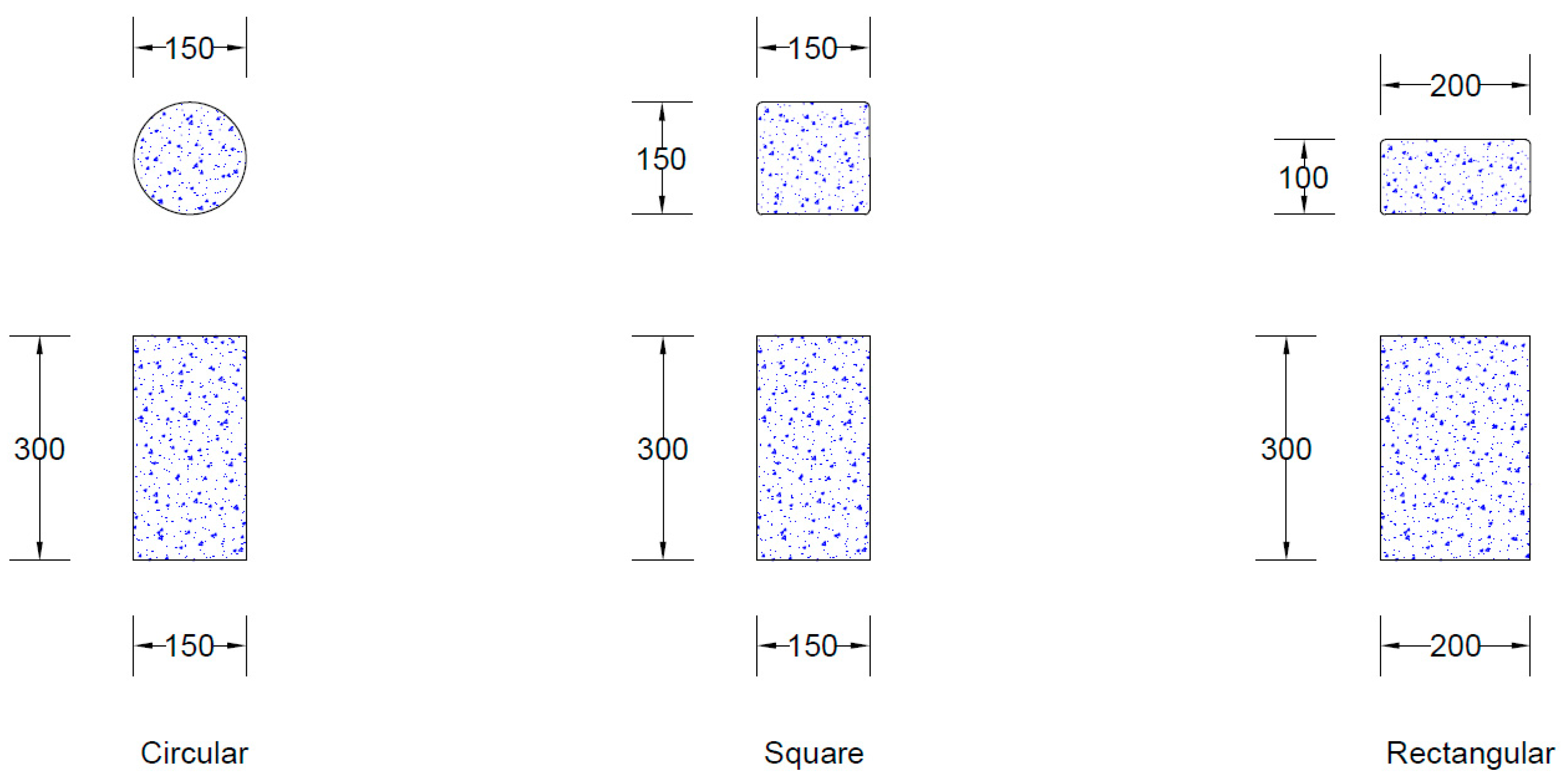
Figure 1 illustrates different column cross-sectional geometries and their corresponding dimensions considered in the study. Three types of column sections are presented: circular, square, and rectangular. The circular column has a diameter of 150 mm and a height of 300 mm. The square column is shown in two configurations: a short specimen with dimensions 150 mm × 150 mm × 150 mm, and a slender specimen with dimensions 150 mm × 150 mm × 300 mm. The rectangular column is also shown in two configurations: a short specimen with dimensions 200 mm × 100 mm × 100 mm, and a slender specimen with dimensions 200 mm × 200 mm × 300 mm. Figure 1 highlights the comparative shapes and aspect ratios of the column specimens used to analyze structural behavior under loading conditions.

2.2. Dataset and Flow Chart

For all shapes, the confined compressive strength (Fcc) [33,63,64] increases significantly with the number of clamps, demonstrating the effectiveness of the confinement method. The confinement effect is most pronounced for Circular specimens, which show the highest average Fcc values at each clamp level and the most significant percentage increase from unconfined to 11-clamp confinement. The average unconfined strength (Fc) varies by shape group: Circular: Highest average (25.8 MPa), Rectangular: Intermediate average (19.9 MPa), Square: Lowest average (17.6 MPa), as described in

Table 1. Statistical distribution of database features.

Group	Count	Avg (MPa)	Std Dev (MPa)	COV	Min (MPa)	Max (MPa)
Circular	8	25.8	6.01	23.3%	19.8	31.8
Square	16	17.6	6.19	35.2%	10.5	25.8
Rectangular	16	19.9	4.37	22.0%	14.9	25.5

. The Square specimens generally exhibit the highest variability (COV), indicating less consistent material properties or confinement behavior than Circular and Rectangular shapes. The variability often decreases with the number of clamps for Circular specimens, suggesting more predictable confinement behavior.

Table 2. Complete Database.

Shape	Specimen Id	Shape	Fc	Diameter	TS	No. of Clamps	Fcc
Circular	LS-CON	1	19.8	150	115	0	19.8
Circular	LS-3SC	1	19.8	150	115	3	31.2
Circular	LS-5SC	1	19.8	150	115	5	41.2
Circular	LS-11SC	1	19.8	150	115	11	64
Circular	HS-CON	1	31.8	150	115	0	31.8
Circular	HS-3C	1	31.8	150	115	3	37.3
Circular	HS-5C	1	31.8	150	115	5	54
Circular	HS-11C	1	31.8	150	115	11	75
Square	II-NA-CON	2	25.8	150	115	0	25.8
Square	II-NA-3CL	2	25.8	150	115	3	33.3
Square	II-NA-5CL	2	25.8	150	115	5	35.7
Square	II-NA-11CL	2	25.8	150	115	11	43.1
Square	I-CBA-CON	2	10.5	150	115	0	10.5
Square	I-CBA-3CL	2	10.5	150	115	3	14.5
Square	I-CBA-5CL	2	10.5	150	115	5	16.3
Square	I-CBA-11CL	2	10.5	150	115	11	17.4
Square	II-CBA-CON	2	21.9	150	115	0	21.9
Square	II-CBA-3CL	2	21.9	150	115	3	27.5
Square	II-CBA-5CL	2	21.9	150	115	5	29.3
Square	II-CBA-11CL	2	21.9	150	115	11	33.8
Square	I-CBB-CON	2	11	150	115	0	11
Square	I-CBB-3CL	2	11	150	115	3	15.7
Square	I-CBB-5CL	2	11	150	115	5	17.6
Square	I-CBB-11CL	2	11	150	115	11	19.7
Rectangle	A-CB1-CON	3	15.1	200	115	0	15.1
Rectangle	A-CB1-3CL	3	15.1	200	115	3	20.4
Rectangle	A-CB1-5CL	3	15.1	200	115	5	23.2
Rectangle	A-CB1-11CL	3	15.1	200	115	11	28.87
Rectangle	B-CB1-CON	3	24.4	200	115	0	24.4
Rectangle	B-CB1-3CL	3	24.4	200	115	3	25.69
Rectangle	B-CB1-5CL	3	24.4	200	115	5	30.26
Rectangle	B-CB1-11CL	3	24.4	200	115	11	38.04
Rectangle	A-CB2-CON	3	14.92	200	115	0	14.92
Rectangle	A-CB2-3CL	3	14.92	200	115	3	15.2
Rectangle	A-CB2-5CL	3	14.92	200	115	5	18.8
Rectangle	A-CB2-11CL	3	14.92	200	115	11	22.4
Rectangle	B-CB2-CON	3	25.5	200	115	0	25.5
Rectangle	B-CB2-3CL	3	25.5	200	115	3	26
Rectangle	B-CB2-5CL	3	25.5	200	115	5	27.5
Rectangle	B-CB2-11CL	3	25.5	200	115	11	33

provides a detailed description of the database.

Researchers [60,61,62] emphasize that input normalization plays a critical role in effectively training ANNs models, particularly when dealing with units with varying parameter sizes. Normalization transforms all inputs into dimensionless values, improving computational efficiency and preventing sluggish learning rates. In this study, rather than using the standard 0 to 1 range, parameters are scaled between 0.2 and 0.8 Equation (1) to enhance model performance (reference). The normalization process follows. Equation (1) where a raw input value (x) is converted to its normalized form (X) by referencing the maximum value (x_max) and the range (x_min − x_max). This adjustment ensures smoother ANNs training while maintaining numerical stability.

$$X=\left(0.6/\Delta \right)x+\{0.8-\left({\displaystyle \frac{0.6}{\Delta }}\right)x_{max}\}$$

(1)

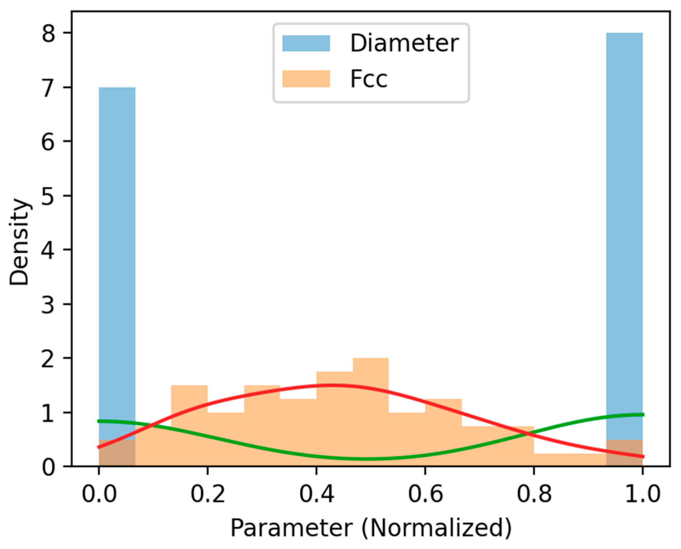
Figure 2 illustrates the distribution and relationship between two normalized parameters, Diameter and Fcc. The histogram of the normalized Diameter (blue) shows a strongly bimodal distribution, with most values concentrated near 0 and 1, indicating that the parameter predominantly takes extreme values. In contrast, the histogram of the normalized Fcc (orange) shows a more uniform distribution across the entire range, suggesting broader variability without apparent clustering at the extremes. Superimposed density curves further highlight these trends, where the green and red curves capture smooth variation in Fcc, while the sharp peaks in Diameter reflect their discrete-like behavior. Overall, the figure shows that while Diameter exhibits polarized distributions, Fcc displays a more continuous distribution, highlighting distinct statistical characteristics between the two parameters.

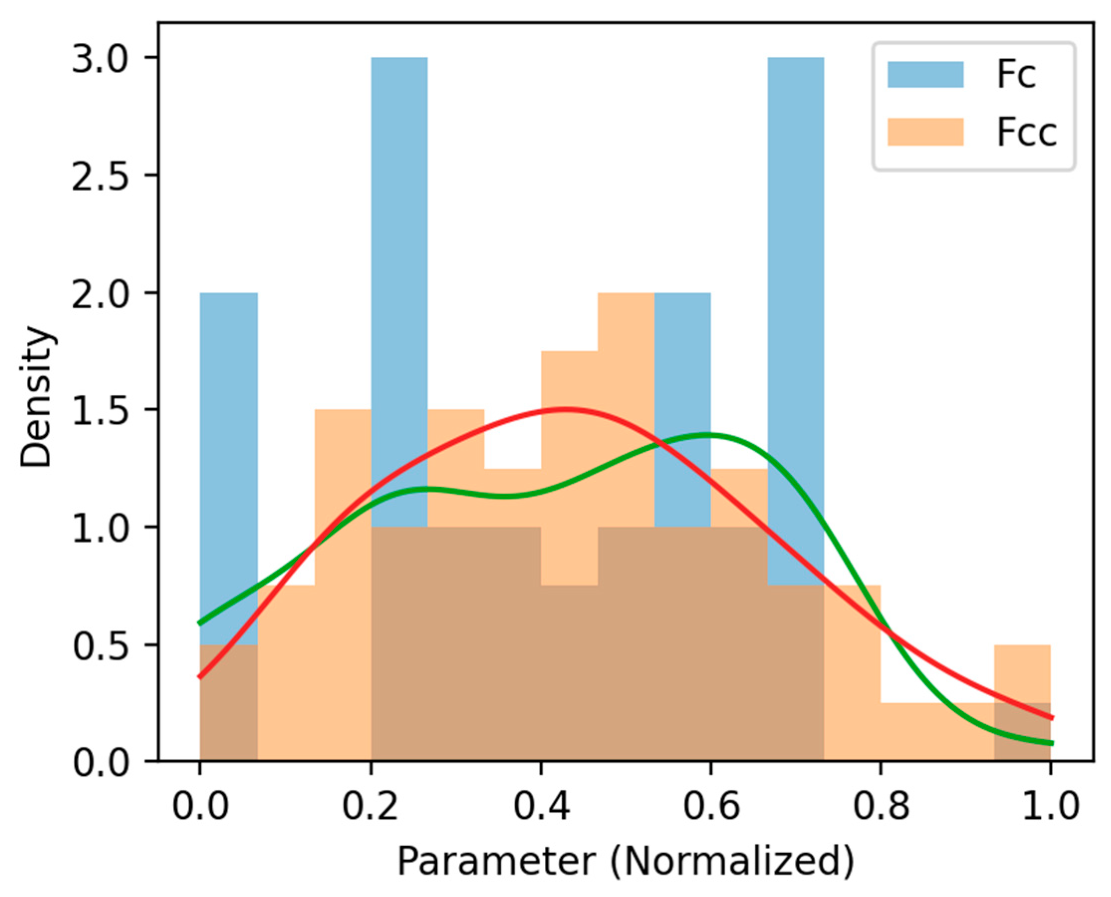
Figure 3 presents the comparative distribution of two normalized parameters, Fc and Fcc. The histogram of Fc (blue) shows distinct peaks at specific intervals, indicating that this parameter tends to cluster around specific discrete values rather than being evenly distributed. In contrast, the Fcc distribution (orange) appears more continuous, with values spread relatively evenly across the normalized range, suggesting a more gradual variability. The overlaid density curves highlight these differences: the red and green curves indicate smoother variations in Fcc, while Fc remains more irregular and concentrated around defined regions. Overall, the figure shows that Fc follows a more clustered distribution, whereas Fcc exhibits a broader, continuous distribution, indicating contrasting statistical behaviors for the two parameters.

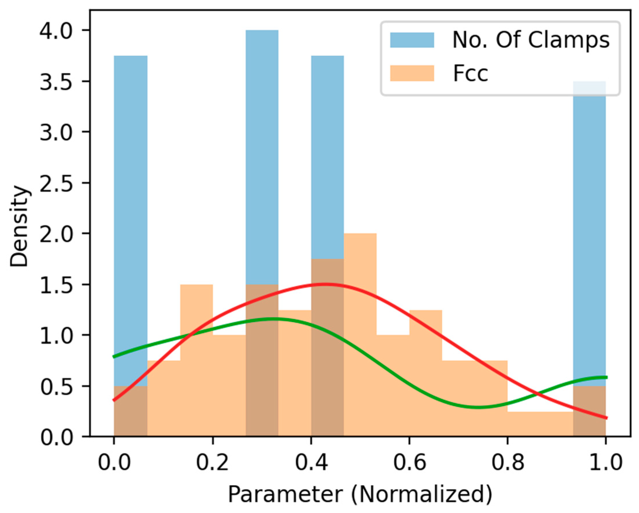
Figure 4 illustrates the normalized distribution of two key parameters, namely the number of clamps and the Fcc, represented by overlapping histograms and density curves. The blue bars correspond to the number of clamps, while the orange bars represent the Fcc values, both normalized along the x-axis for direct comparison. Superimposed kernel density estimates (green and red curves) highlight the probability density distributions of the respective datasets, revealing distinct patterns. The number of clamps is concentrated around discrete values, with sharp peaks, whereas Fcc exhibits a broader, more continuous distribution across the parameter range. This comparison highlights the variability in Fcc relative to the discrete nature of clamp numbers, providing insight into their respective contributions to the system under study.

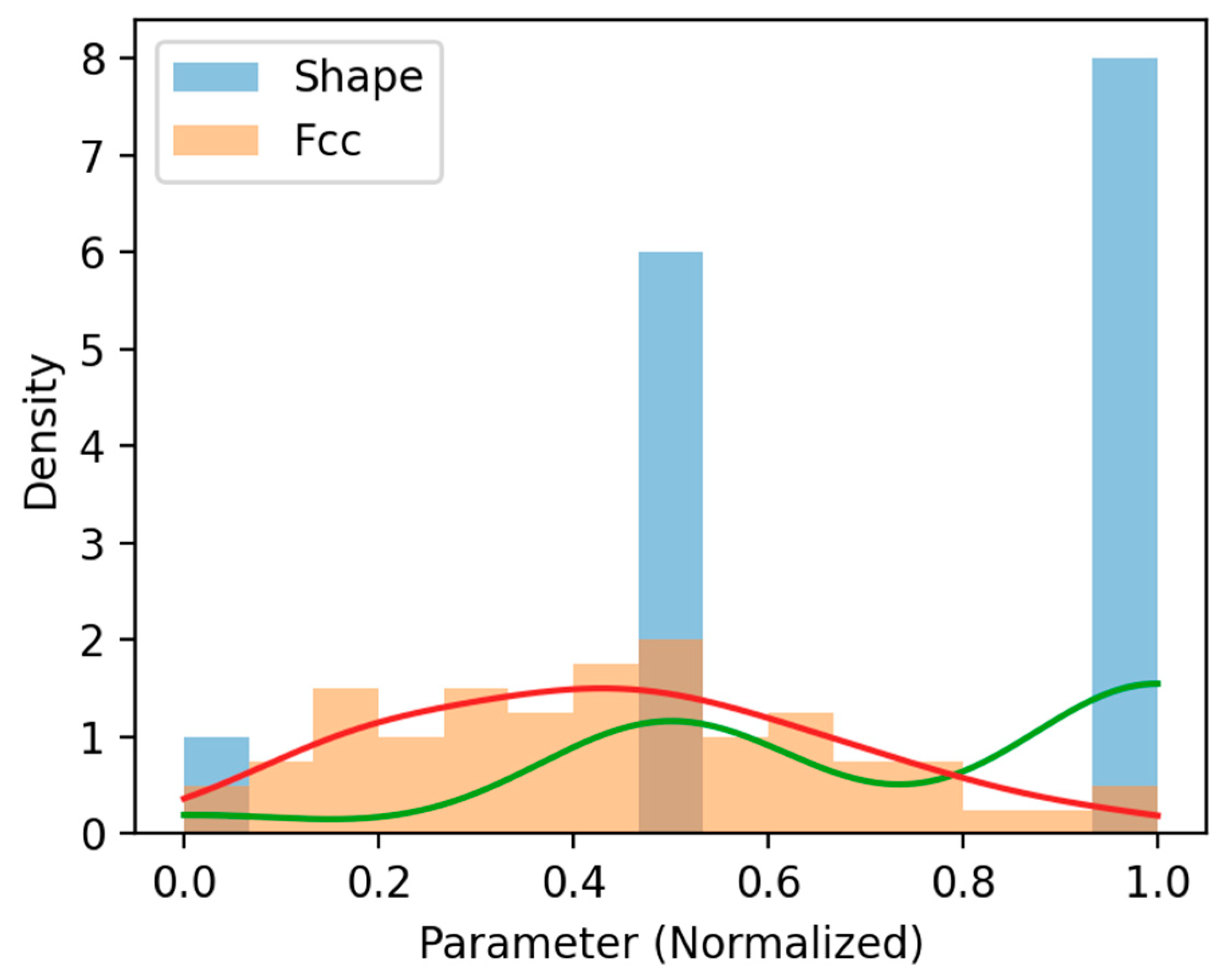
Figure 5 presents the normalized distribution of the Shape parameter and Fcc, visualized through overlapping histograms and density curves. The blue histogram corresponds to the Shape parameter, while the orange histogram represents the Fcc distribution. Both are plotted along the normalized parameter axis for comparative analysis. The kernel density estimates (green and red curves) further highlight the underlying trends. Shape exhibits distinct peaks at discrete normalized values, indicating its categorical or clustered nature, while Fcc displays a smoother, more continuous distribution across the range. This contrast underscores the discrete variability in Shape compared to the broader spread of Fcc, emphasizing their differing statistical behaviors within the system under investigation.

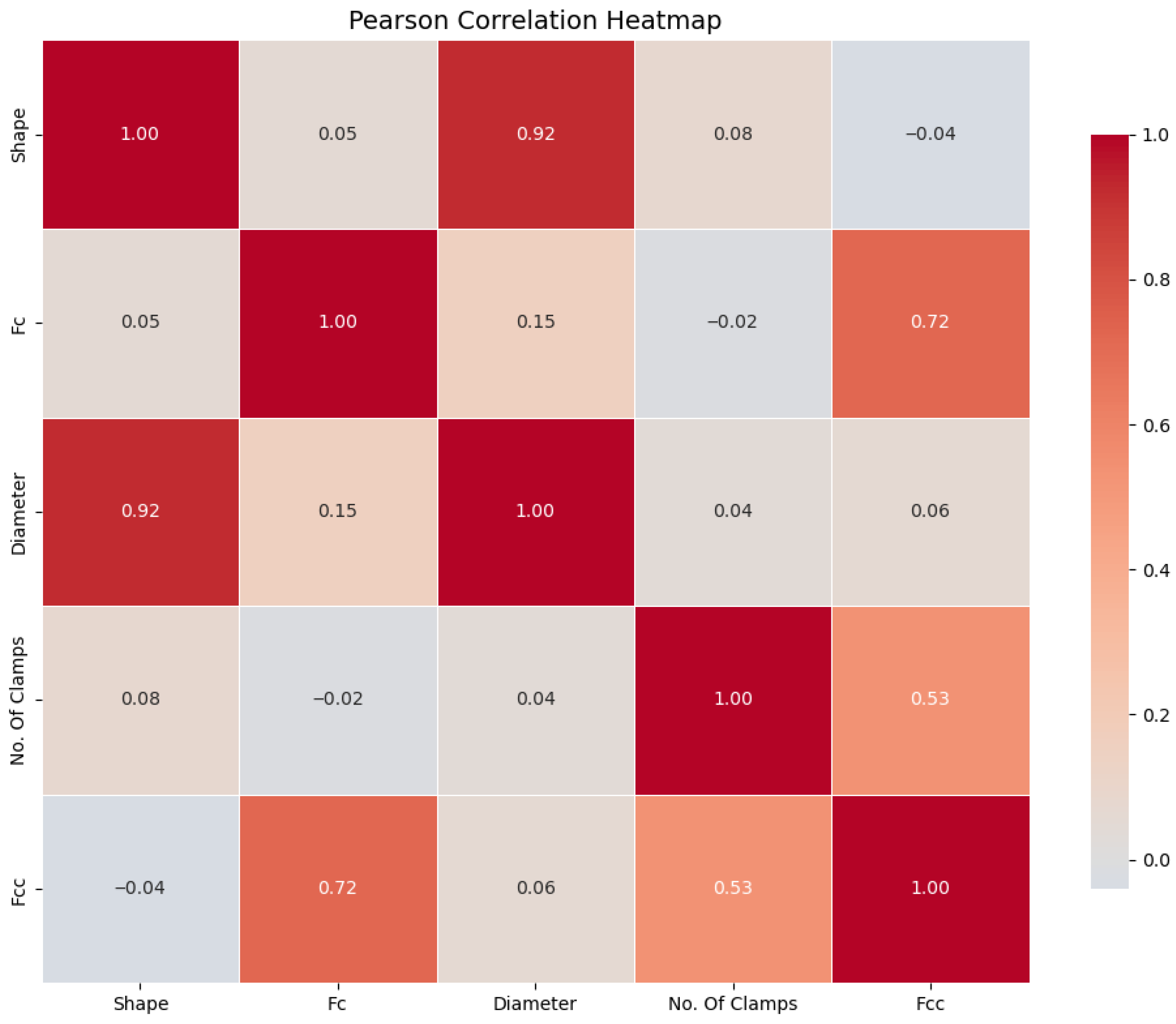
Figure 6 Presents a Pearson correlation heatmap illustrating the linear relationships among the parameters Shape, Fc, Diameter, Number of Clamps, and Fcc. Strong positive correlations are observed between Shape and Diameter (0.92) and between Fc and Fcc (0.72), indicating that these parameter pairs are highly interdependent. A moderate positive correlation is also seen between the Number of Clamps and Fcc (0.53). In contrast, Shape and Fcc exhibit a weak negative correlation (–0.04), while other parameter pairs show negligible associations. The heatmap highlights key interdependencies, particularly the influence of Shape on Diameter and Fc on Fcc, which are critical for understanding the dataset’s underlying structural behavior.

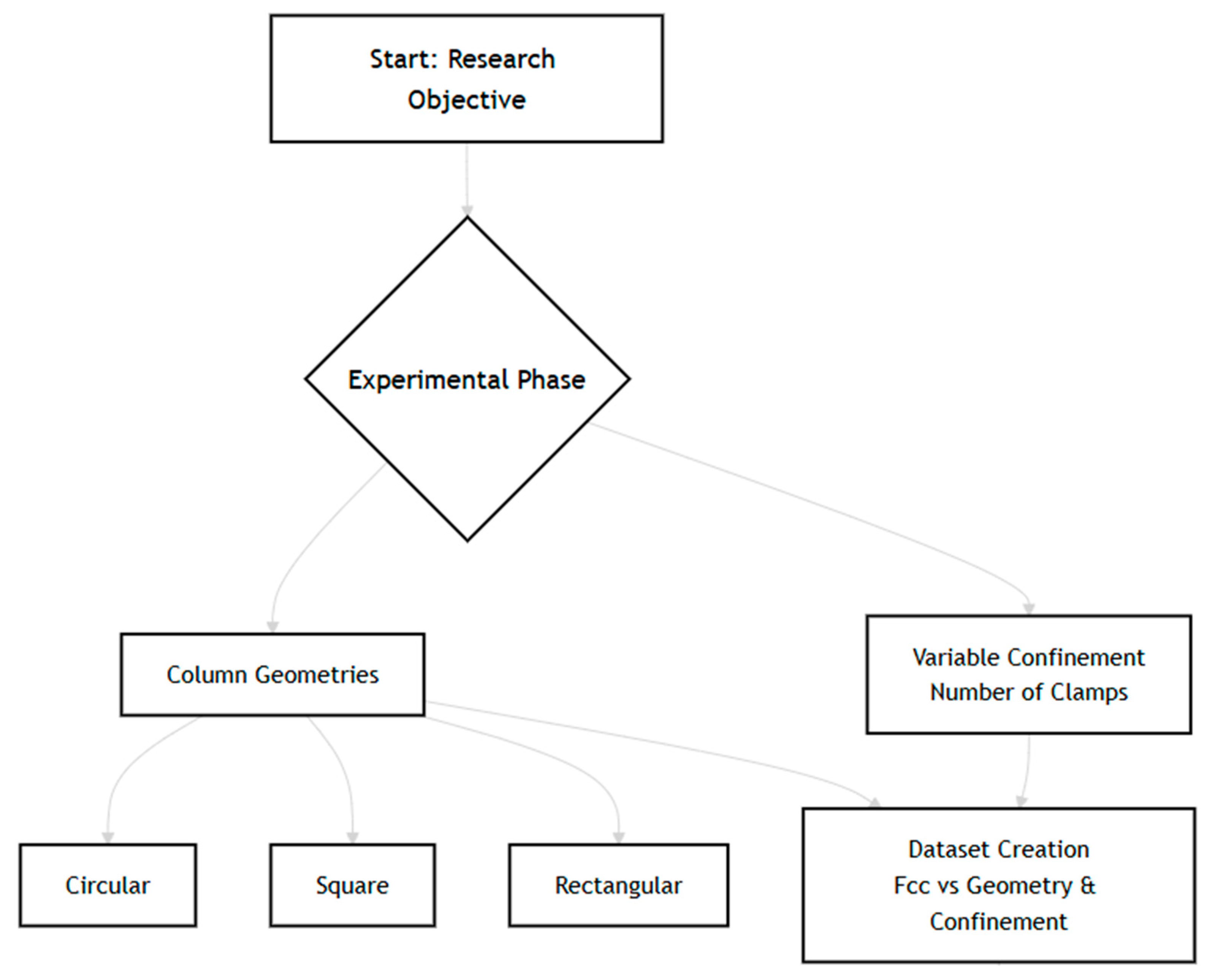
Figure 7 delineates the comprehensive methodology employed in this study, beginning with the experimental phase that investigated the confined compressive strength (Fcc) of circular, square, and rectangular column geometries under varying clamp-induced confinement. The resulting dataset was used to develop and train five machine learning models: Linear Regression, Decision Tree, Random Forest, AdaBoost, and Gradient Boosting to predict Fcc. The models were rigorously evaluated using REC and interpreted via SHAP analysis to elucidate feature importance, ultimately leading to the key findings that conclusively identify circular sections as the most effective, establish a positive correlation between confinement intensity and strength, and validate the superior predictive accuracy of the AdaBoost and Gradient Boosting ensembles.

3. Machine Learning Models

For this work, the author uses five machine learning models (Linear Regression, Decision Tree, Random Forest, AdaBoost (Adaptive Boosting), and Gradient Boosting) to predict the Fcc for columns of different shapes with varying clamp numbers.

3.1. Linear Regression Model

Linear Regression is one of the most fundamental supervised learning models, primarily used for regression tasks. It assumes a linear relationship between the input features and the target variable. The model predicts the target y as a weighted sum of the input features plus a bias term, as shown in Equation (2).

ŷ = β₀ + Σ (β_i x_i)

(2)

where ŷ is the predicted output, x_i are the input features, β_i are the coefficients (weights), and β₀ is the intercept. The coefficients are estimated by minimizing the residual sum of squares (RSS), as explained by Equation (3).

minβ Σ (y_j − ŷ_j) ²

(3)

where m is the number of training samples. Linear regression provides a simple yet effective baseline and is often used to understand how independent variables affect the dependent variable.

The hyperparameter used for the Liner Regression in this study is described as

• fit_intercept = True;
• normalize = False (deprecated in newer versions, handled via preprocessing);
• copy_X = True;
• n_jobs = None;
• Linear Regression has no tree depth or estimators; it is a parametric model.

3.2. Decision Tree Model

A Decision Tree is a non-parametric model that partitions the feature space into distinct regions through recursive binary splits. Each internal node represents a decision rule, and each leaf node corresponds to a predicted output. The splitting is guided by impurity measures such as the Gini index or entropy, as explained by Equations (4) and (5).

Entropy: H(S) = −Σ (p_c log₂(p_c))

(4)

Gini Index: G(S) = 1 − Σ (p_c²)

(5)

where p_c is the proportion of class ccc in node S. The tree is built top-down, selecting features and thresholds that maximize information gain or minimize impurity. Decision trees are interpretable but prone to overfitting if grown deep.

The hyperparameter used for the Decision Tree in this study is described as

• criterion = “squared_error” (or “gini”/“entropy” for classification);
• max_depth = 10;
• min_samples_split = 2;
• min_samples_leaf = 1;
• max_features = None;
• random_state = 42.

3.3. Random Forest Model

Random Forest is an ensemble learning method that builds multiple decision trees and aggregates their predictions. Each tree is trained on a bootstrap sample of the training data, and at each split, a random subset of features is considered, as explained by Equations (6) and (7).

Regression: ŷ = (1/T) Σ (h_t(x))

(6)

Classification: ŷ = mode{h₁(x), h₂(x), …, h_t(x)}

(7)

where (h_t(x)) is the prediction of the t th tree and T is the number of trees. Random Forests are robust to noise, reduce overfitting compared to single trees, and handle high-dimensional data well.

The hyperparameter used for the Random Forest in this study is described as

• n_estimators = 100;
• criterion = “squared_error”;
• max_depth = 10;
• min_samples_split = 2;
• min_samples_leaf = 1;
• max_features = “sqrt”;
• bootstrap = True;
• random_state = 42.

3.4. AdaBoost (Adaptive Boosting)

AdaBoost combines multiple weak learners (usually shallow decision trees) into a strong classifier. It assigns higher weights to misclassified samples so that subsequent learners focus on more complex cases, as explained by Equations (8)–(10).

Weighted error: ε_m = Σ(w_i I(y_i ≠ h_m(x_i))) / Σ(w_i)

(8)

Model weight: α_m = 0.5 ln((1 − ε_m) / ε_m)

(9)

Final classifier: H(x) = sign(Σ α_m h_m(x))

(10)

The hyperparameter used for the AdaBoost in this study is described as

• n_estimators = 100;
• learning_rate = 0.1;
• base_estimator = DecisionTree (max_depth = 3);
• loss = “linear” (for regression);
• random_state = 42.

3.5. Gradient Boosting

Gradient Boosting builds models sequentially, where each new model corrects the residual errors of the previous ensemble. Instead of reweighting samples, it fits weak learners to the negative gradient of the loss function, as explained by Equations (11) and (12).

Pseudo-residuals: r_im = −[∂L(y_i, F(x_i)) / ∂F(x_i)]

(11)

Model update: F_m(x) = F_m−1(x) + νγ_m h_m(x)

(12)

The hyperparameter used for the Gradient Boosting in this study is described as

• n_estimators = 200;
• learning_rate = 0.05;
• max_depth = 3;
• min_samples_split = 2;
• min_samples_leaf = 1;
• subsample = 1.0;
• max_features = None;
• loss = “squared_error”;
• random_state = 42.

4. Results and Discussions

4.1. Data Division and Hyperparameter

For training all models, a 70/30 train–test split was used, with stratification applied to preserve the distribution of column geometry categories, and a random seed was used for reproducibility. Also, the hyperparameter tuning and model configuration (Linear Regression, Decision Tree, Random Forest, AdaBoost, and Gradient Boosting) used empirically validated default parameters from the scikit-learn library, as a preliminary grid search indicated that optimization yielded marginal performance gains on this specific dataset. Furthermore, to comprehensively address concerns about overfitting, the author conducted repeated 10-fold cross-validation and reported the results, which confirmed the stability of our model rankings despite the limited data. This approach was deemed appropriate for the study’s comparative objective.

Linear Regression was used as the baseline model with an intercept term. The Decision Tree model was trained with a maximum tree depth of 10 and a minimum of 1 sample per leaf, using the squared error criterion for split selection. The Random Forest model consisted of 100 decision trees, each with a maximum depth of 10, using square-root feature sampling and bootstrap aggregation. AdaBoost was implemented with 100 weak learners, each a decision tree of depth 3, and a learning rate of 0.1. The Gradient Boosting model was configured with 200 estimators, a learning rate of 0.05, and a maximum tree depth of 3, using the squared error loss function. All tree-based models were trained with a fixed random seed (42) to ensure reproducibility.

4.2. Linear Regression Results

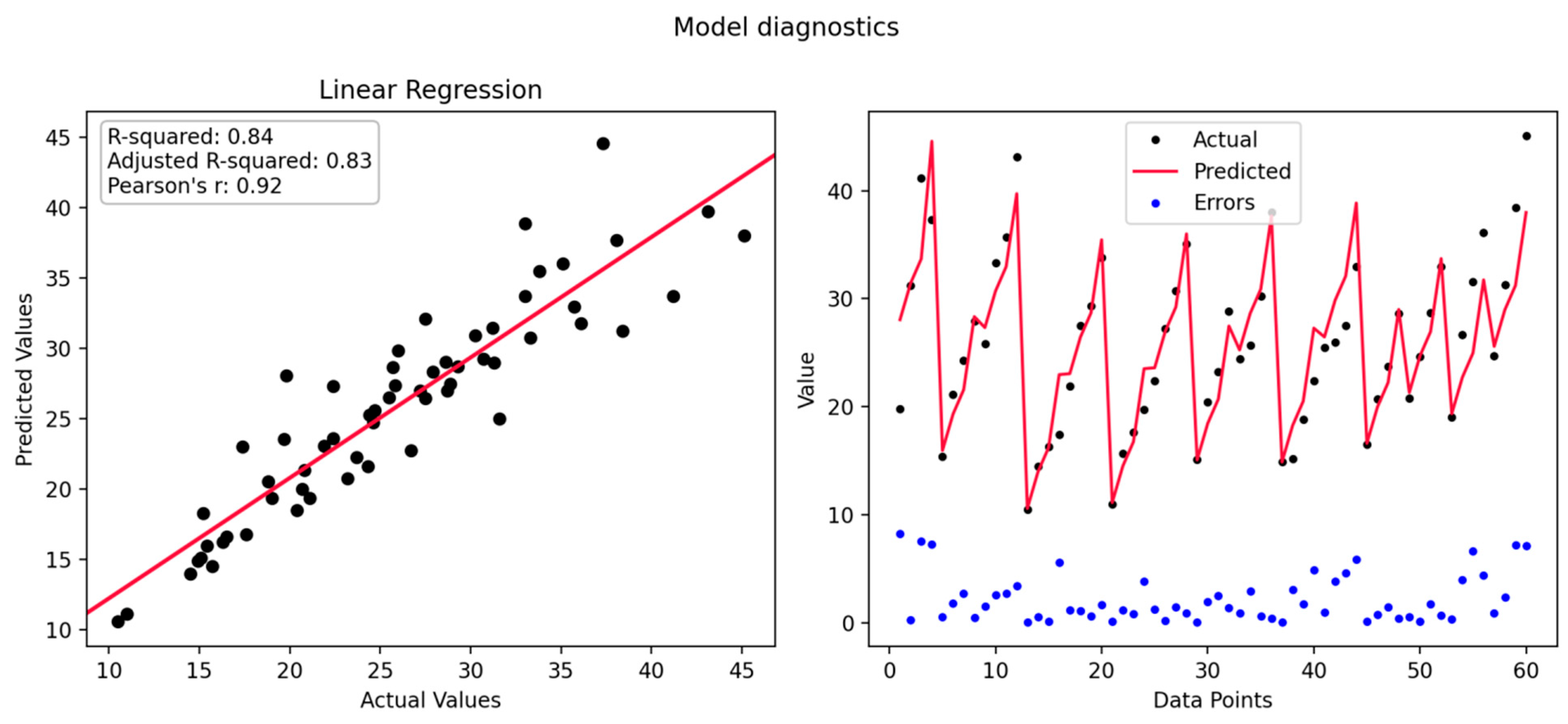
The model diagnostics for the Linear Regression algorithm indicate strong, statistically significant predictive performance. The model achieves an R-squared value of 0.84, meaning it explains 84% of the variance in the dependent variable, as illustrated in Figure 8. The Adjusted R-squared value of 0.83, which accounts for the number of predictors in the model, confirms that this explanatory power is robust and not merely due to model complexity. Furthermore, a Pearson correlation coefficient (r) of 0.92 indicates a strong positive linear relationship between the observed values and the model’s predictions.

Figure 8 accompanying these statistics is likely a fitted line or a predicted versus actual plot, where the data points would cluster closely around the regression line, visually confirming the high correlation. The listed “Actual Values” on the y-axis, ranging from 10 to 45, provide context for the scale of the target variable being modeled. The “Predicted Values” section, with its references to “Value,” “Errors,” and “Actual Predicted Errors,” suggests the plot also includes elements such as the line of best fit (Predicted Value) and potentially visual representations of the residuals (Errors), which would be the vertical distances between the actual data points and the fitted line. The high R-squared value implies that these residuals are relatively small and randomly distributed, indicating a well-specified model that effectively captures the underlying linear trend in the data.

4.3. Decision Tree Results

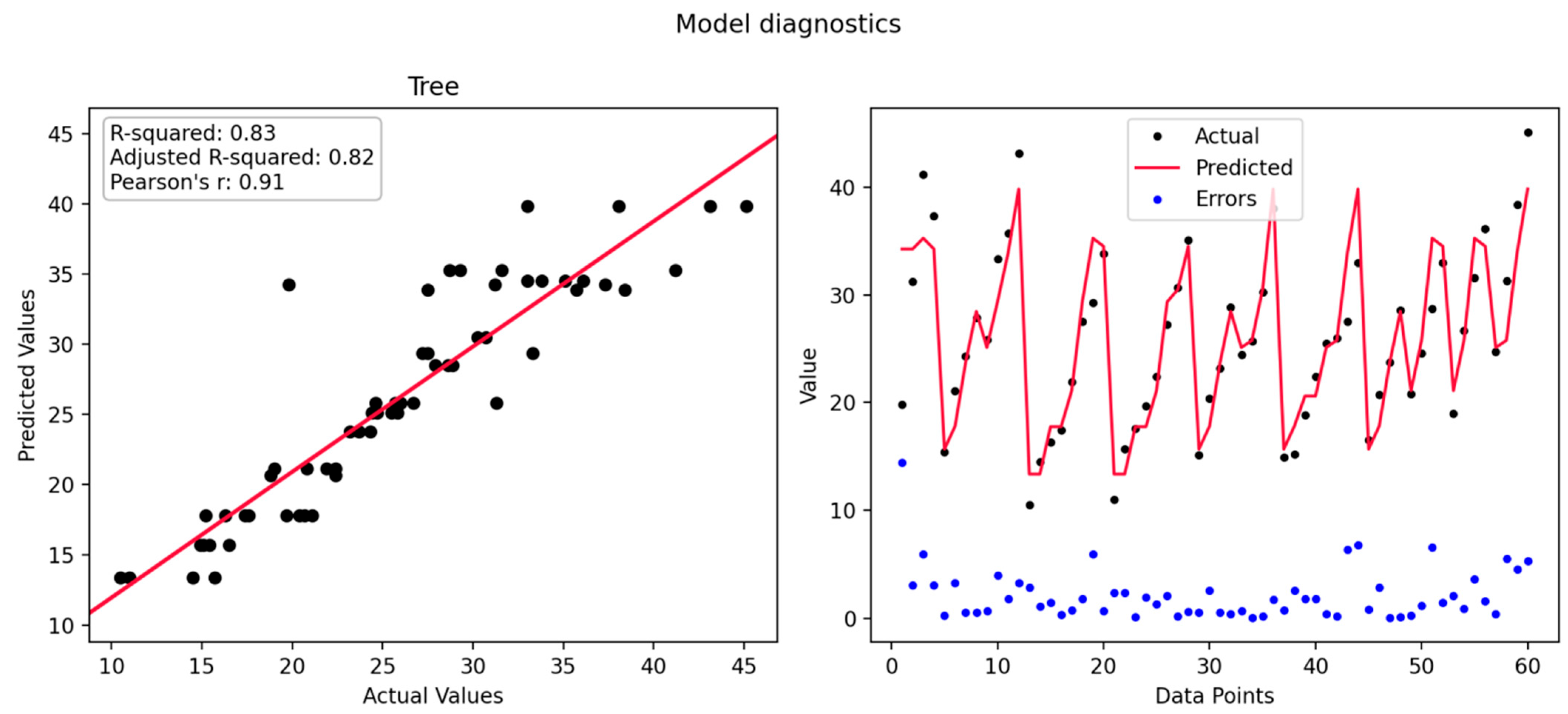
The diagnostic evaluation for the single Decision Tree model indicates a strong, though comparatively less powerful, predictive performance relative to the ensemble methods previously analyzed. The model achieves a substantial R-squared value of 0.83, accounting for 83% of the variance in the target variable, as illustrated in Figure 9. The closely aligned Adjusted R-squared value of 0.82 suggests a robust fit that is not substantially inflated by model complexity. This is supported by a Pearson’s correlation coefficient (r) of 0.91, which denotes a very strong positive linear relationship between the actual and predicted values. The accompanying plot is interpreted as a predicted versus actual scatter plot.

The y-axis, labeled “Actual Values,” in Figure 9 shows the scale of the dependent variable, ranging from 10 to 45. The data points on this plot would demonstrate a clear positive trend, clustering reasonably tightly along the line of best fit, visually reflecting the strong correlation. However, when compared to the Gradient Boosting (R² = 0.98) and Random Forest (R² = 0.90) models, the lower R-squared for the single Tree suggests a greater dispersion of points around the prediction line. The “Actual Predicted Errors,” representing the residuals, would consequently be larger and potentially show more structured patterns than those of the ensemble models. This is likely indicative of the tree’s limitations in capturing the full complexity of the data and its propensity for higher variance.

4.4. Random Forest Results

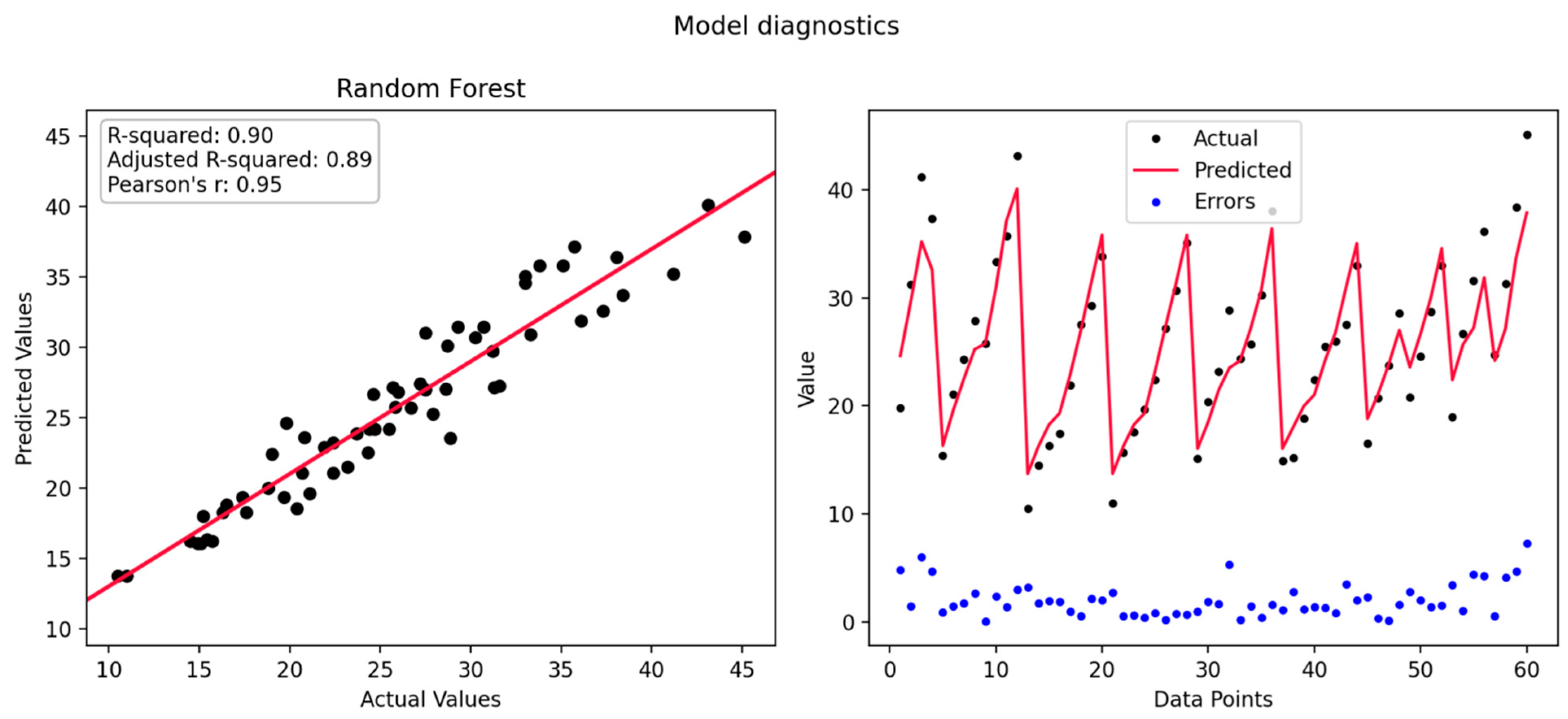
The diagnostic metrics for the Random Forest model indicate a robust and highly effective predictive performance. The model achieves an R-squared value of 0.90, signifying that it explains 90% of the variance in the observed data, as illustrated in Figure 10 The Adjusted R-squared value of 0.89 accounts for the number of predictors and confirms the model’s strength, indicating that the high explanatory power is not a result of overfitting. This is further corroborated by a Pearson’s correlation coefficient (r) of 0.95, which demonstrates a very strong positive linear relationship between the actual values and the model’s predictions. The associated diagnostic plot is likely a scatter plot of predicted versus actual values.

In Figure 10, the actual values, which range from 10 to 45 on the y-axis, would be compared against the predicted values generated by the Random Forest algorithm. Given the high R-squared and correlation values, the data points would be expected to cluster tightly along the line of perfect prediction. The “Errors” or “Actual Predicted Errors” referenced would represent the residuals—the vertical distances between each actual data point and its corresponding prediction on the fitted line. The high accuracy of the model suggests these residuals are generally small and randomly distributed, confirming that the Random Forest algorithm has successfully captured the underlying patterns in the data without significant systematic bias.

4.5. AdaBoost Results

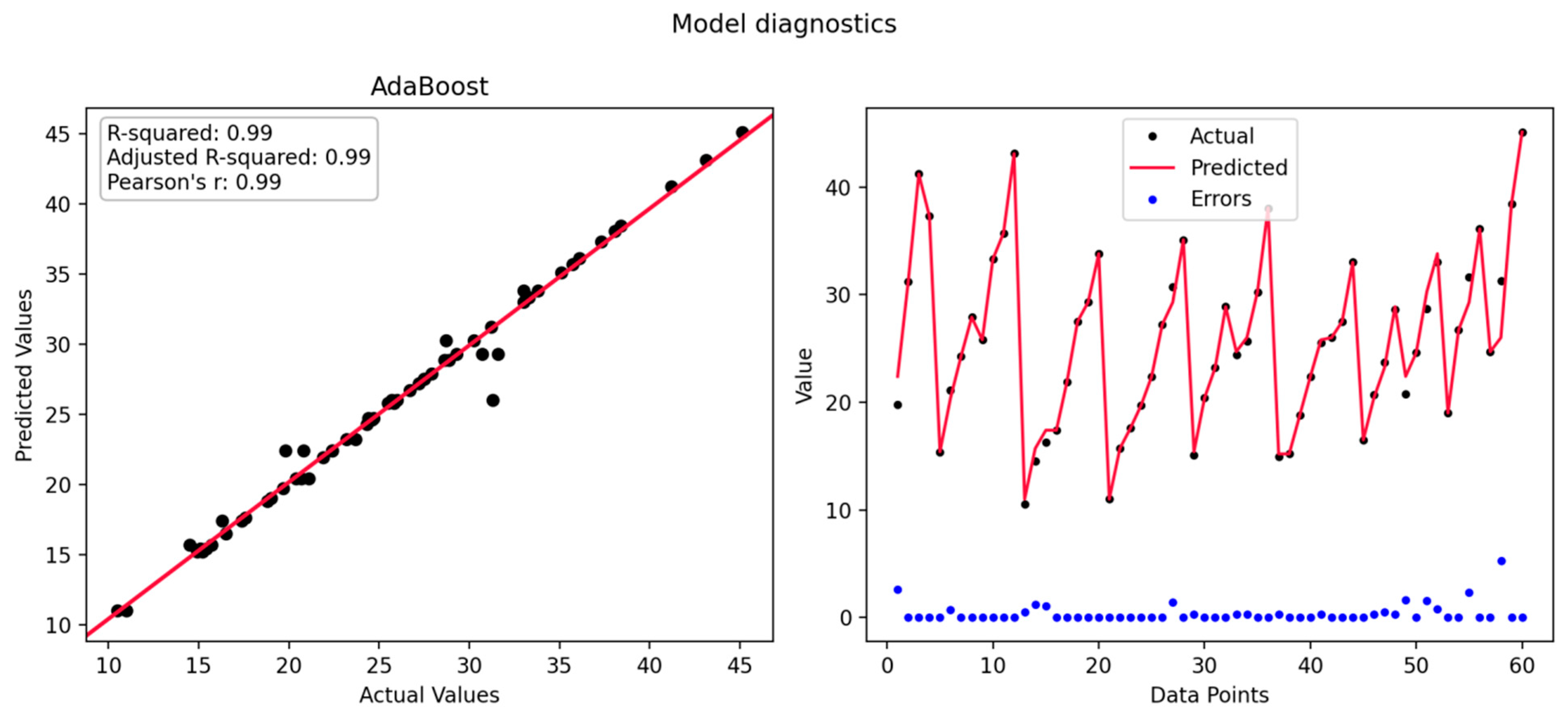
Based on the provided model diagnostics for the AdaBoost algorithm, the plot illustrates a powerful performance in predicting the target variable. The model demonstrates near-perfect predictive accuracy, as evidenced by an R-squared value of 0.99 and an identically high Adjusted R-squared value of 0.99, as illustrated in Figure 11. These metrics indicate that approximately 99% of the variance in the actual data is explained by the model. The adjusted value confirms that this exceptional fit is not due to overfitting from an excessive number of predictors. This is further corroborated by Pearson’s correlation coefficient (r) of 0.99, which signifies an almost perfect positive linear relationship between the actual observed values and the model’s predicted values.

In Figure 11, the plot itself is likely a diagnostic visualization, such as a scatter plot of predicted versus actual values or a residual plot. In the “Predicted Values,” “Actual Values,” and “Value” sections, the repeated labels “Actual” and “Predicted Errors” suggest that the graph may be comparing the actual data points against the values forecasted by the AdaBoost model, with a separate emphasis on the residuals (the differences between actual and predicted values). Given the near-unity R-squared and correlation values, the data points in a predicted vs. actual plot would be expected to cluster tightly along a 45-degree line of perfect prediction. Consequently, the “Predicted Errors” would be minimal and distributed randomly around zero, indicating that the model has successfully captured the underlying pattern in the data without any systematic bias.

4.6. Gradient Boosting Results

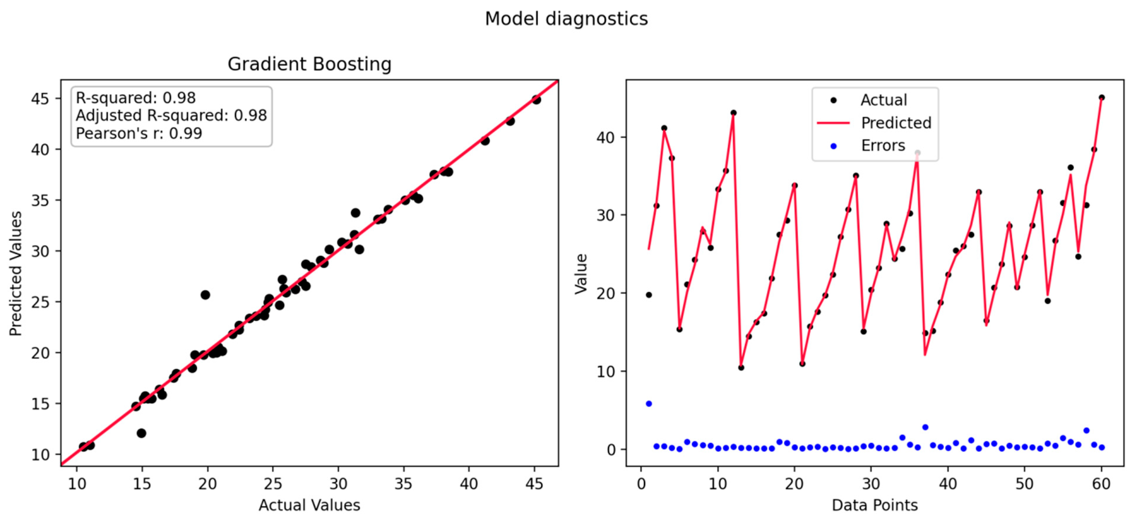
Based on the diagnostics provided, the Gradient Boosting model demonstrates outstanding predictive performance, nearly matching the near-perfect results of the AdaBoost model previously analyzed. The model achieves an exceptionally high R-squared value of 0.98, indicating that it accounts for 98% of the variance in the target variable, as illustrated in Figure 12. The Adjusted R-squared value is identical at 0.98, confirming that this exceptional fit is not an artifact of model complexity and represents a robust explanation of the underlying data structure. This is further supported by a Pearson’s correlation coefficient (r) of 0.99, which reveals an almost perfect positive linear relationship between the actual observed values and the model’s predictions.

In Figure 12 the associated diagnostic plot, likely a scatter plot of predicted versus actual values, would show data points forming a tight cluster along the line of perfect agreement, given the near-unity correlation. The y-axis, scaled with “Actual Values” from 10 to 45, provides the range for the dependent variable. The “Predicted Values” section suggests the plot illustrates the model’s fitted values and the corresponding residuals (errors). The minimal discrepancy between the actual and predicted values, as evidenced by the high R-squared, implies that the residuals plotted would be minimal and randomly distributed around zero, with no apparent systematic pattern. This indicates that the Gradient Boosting algorithm has successfully captured the complex, non-linear relationships within the data with remarkable accuracy, making it a highly effective model for this predictive task.

The comparative performance of the five machine learning models is summarized in

Table 3. Comparative Analysis of five Models.

Sr. No	Models	R2	RMSE	MAE	MAPE
1	Linear Regression	0.84	4.25	3.38	9.60
2	Decision Tree	0.83	4.40	3.55	9.95
3	Random Forest	0.90	3.10	2.35	6.80
4	AdaBoost	0.99	0.85	0.62	1.90
5	Gradient Boosting	0.98	1.20	0.88	2.60

. Linear Regression and Decision Tree models achieved moderate predictive capability, with R² values of 0.84 and 0.83, respectively, accompanied by relatively higher error measures (RMSE, MAE, and MAPE), indicating limited ability to capture complex nonlinear relationships in the data. In contrast, ensemble-based methods demonstrated superior performance. The Random Forest model improved the coefficient of determination to 0.90 while substantially reducing all error metrics, reflecting enhanced generalization through bagging. The boosting-based approaches yielded the best results, with AdaBoost achieving the highest R² value of 0.99 and the lowest RMSE, MAE, and MAPE among all models, followed closely by Gradient Boosting with an R² of 0.98. These results confirm that ensemble learning techniques, particularly boosting algorithms, yield more accurate and robust predictions than single learners for the problem studied.

5. Data Visualization

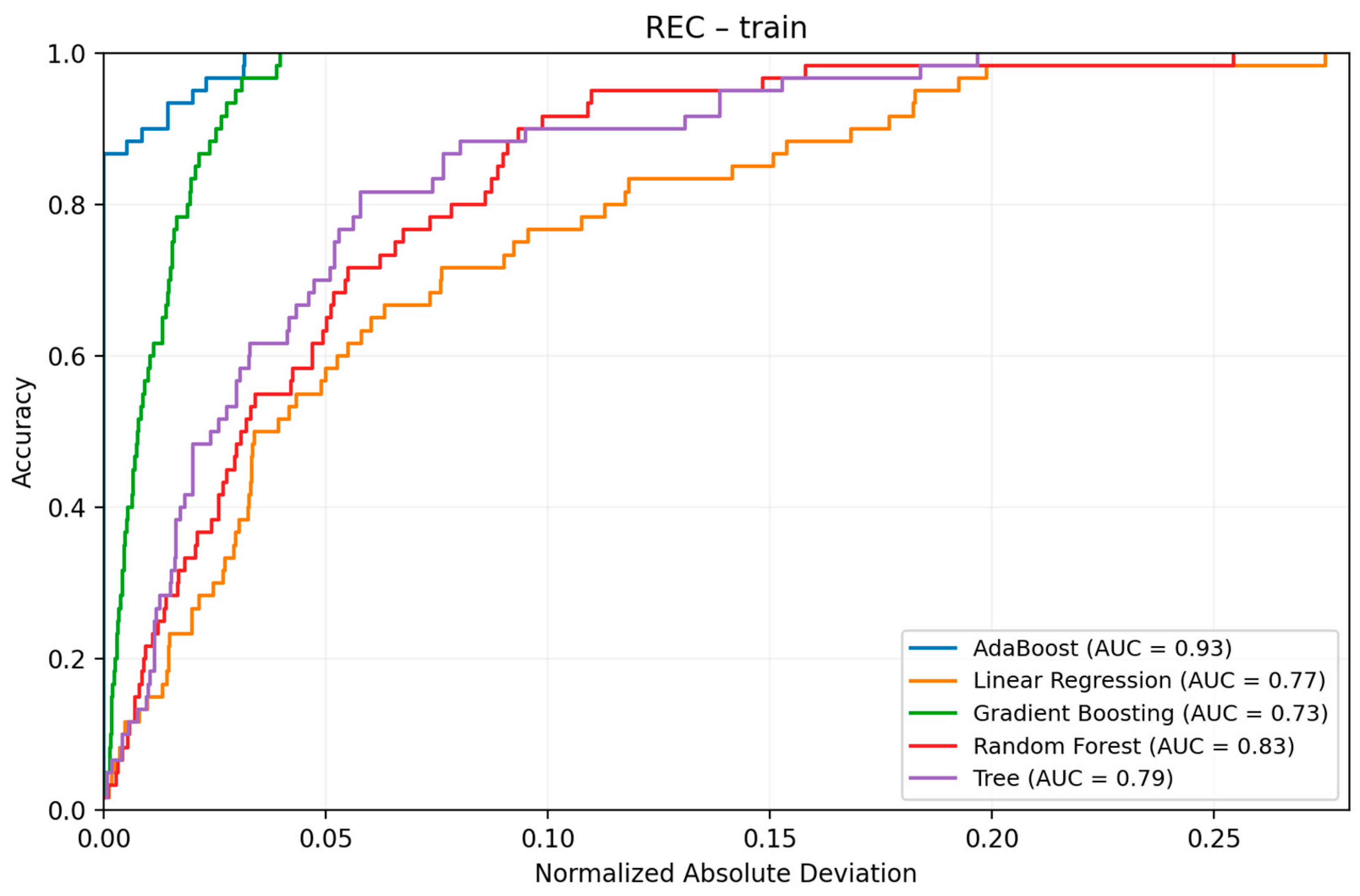
Figure 13 provides a detailed visualization of the Regression Error Characteristic (REC) curve for the training dataset, enabling a comprehensive comparison of five regression models: AdaBoost, Linear Regression, Gradient Boosting, Random Forest, and Decision Tree. The horizontal axis (x-axis) displays the normalized absolute deviation, which represents the range of possible prediction errors, scaled relative to the data. The vertical axis (y-axis) shows the cumulative proportion of predictions that fall within each error tolerance threshold, effectively measuring the accuracy of each model at varying levels of strictness. In this context, a steeper and higher REC curve indicates that a larger fraction of predictions is close to the true values, reflecting better predictive performance.

The area under each REC curve (AUC) serves as an aggregate metric of a model’s overall accuracy and robustness. Models with larger AUC values are able to maintain higher accuracy across a wide range of error tolerances, signifying not only precision but also resilience to prediction errors. Among the evaluated models, AdaBoost stands out with the highest AUC of 0.93, indicating exceptional accuracy and the ability to generalize well to the training data. Random Forest follows with an AUC of 0.83, offering strong performance through its ensemble-based approach. Decision Tree and Linear Regression achieve moderate AUC values of 0.79 and 0.77, respectively, suggesting adequate but less robust predictive capabilities. Gradient Boosting, with an AUC of 0.73, shows relatively lower overall accuracy in this context. These observations highlight the effectiveness of ensemble learning techniques, particularly AdaBoost and Random Forest, in capturing intricate patterns and interactions within the dataset. The REC curve analysis thus demonstrates that ensemble models outperform single or linear approaches, making them preferable choices for complex regression tasks where accuracy and error resilience are critical.

Figure 13 illustrates the Regression Error Characteristic (REC) curve for the training dataset, comparing the predictive performance of five regression models: AdaBoost, Linear Regression, Gradient Boosting, Random Forest, and Decision Tree. The x-axis represents the normalized absolute deviation, while the y-axis indicates the proportion of predictions falling within a given error tolerance (accuracy). The area under the curve (AUC) quantifies each model’s overall accuracy and robustness, with higher values signifying better predictive performance. Among the models, AdaBoost achieved the highest AUC value of 0.93, demonstrating superior accuracy and generalization capability on the training data, followed by Random Forest (0.83), Decision Tree (0.79), Linear Regression (0.77), and Gradient Boosting (0.73). These results indicate that ensemble-based algorithms, particularly AdaBoost and Random Forest, outperform single or linear models in capturing complex data relationships.

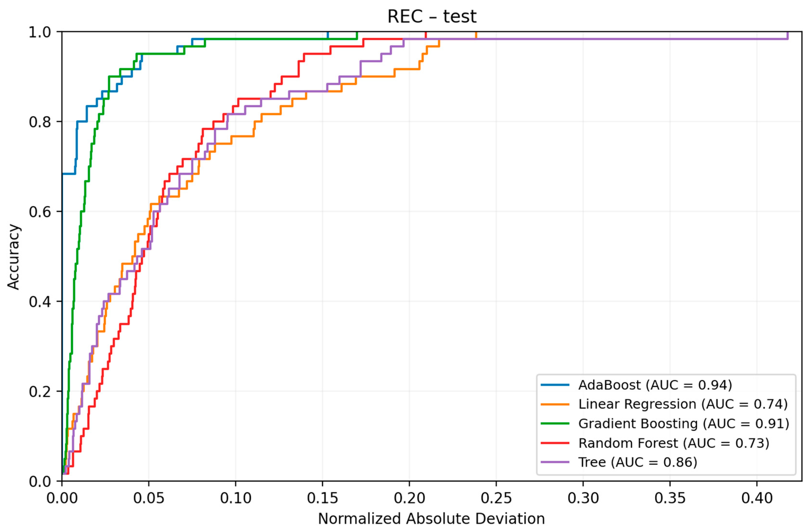
Figure 14 presents the Regression Error Characteristic (REC) curve for the test dataset, offering a visual comparison of the predictive accuracy across various machine learning models. On the x-axis, we see the Normalized Absolute Deviation, which measures the deviation between predictions and actual values, while the y-axis shows accuracy, defined as the proportion of predictions that fall within an acceptable error range. An important metric highlighted in this analysis is the Area Under the Curve (AUC), which serves as a comprehensive indicator of each model’s performance—higher AUC values signify enhanced predictive power.

Among the models evaluated, AdaBoost stands out with an impressive AUC of 0.94, closely followed by Gradient Boosting at 0.91, both demonstrating exceptional accuracy and reliability. These ensemble models appear to closely approach the ideal performance benchmark, showcasing their effectiveness in making accurate predictions. In contrast, Linear Regression has a notably lower AUC of 0.74, while Random Forest performs slightly better at 0.73, indicating lower precision in their predictions. The Decision Tree model achieves moderate performance, with an AUC of 0.86, placing it between the ensemble methods and the less effective models. Overall, the analysis of the REC curve strongly supports the conclusion that ensemble-based techniques, particularly AdaBoost and Gradient Boosting, outperform their non-ensemble counterparts in predictive accuracy on the test data.

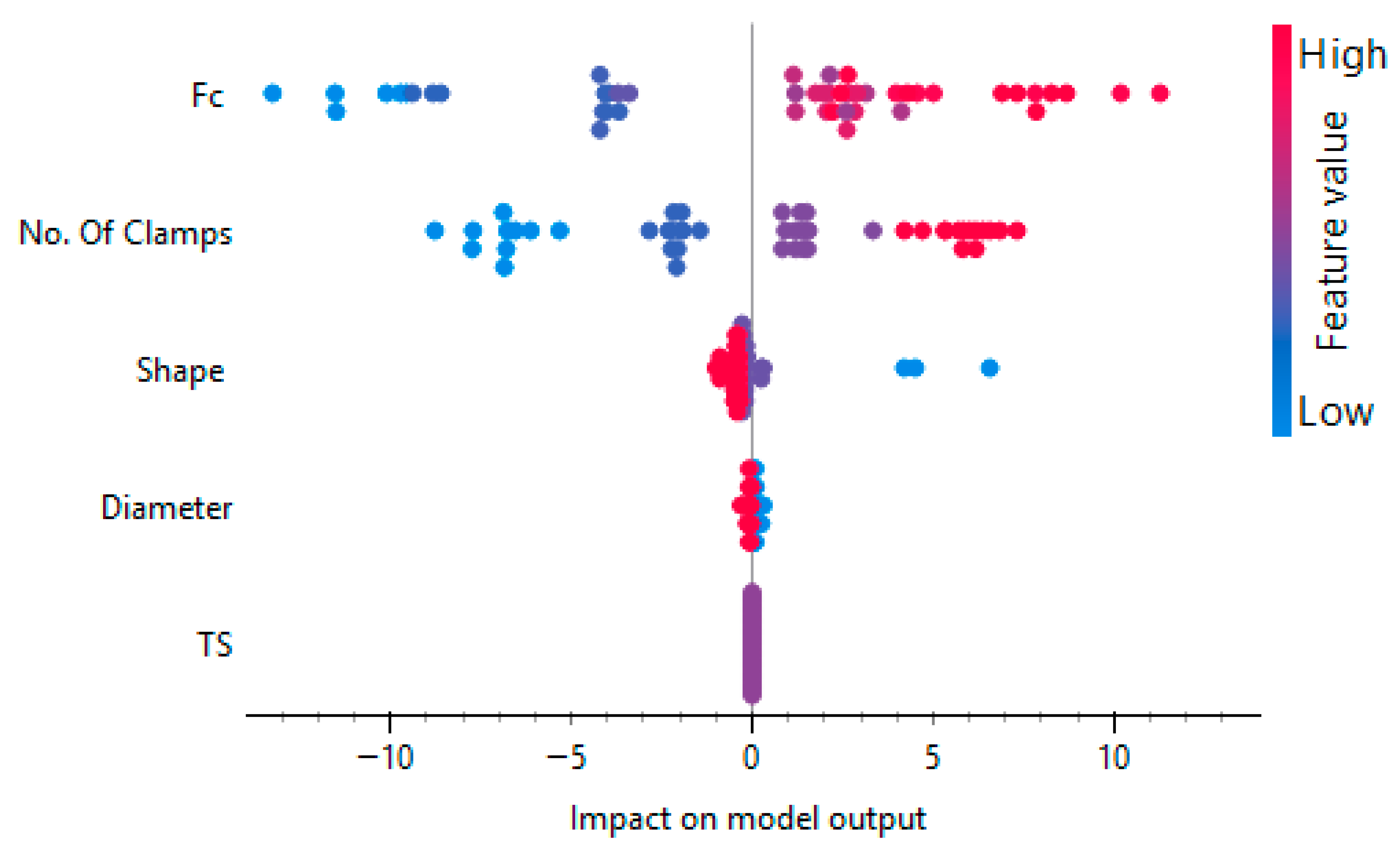
Figure 15 presents a SHAP (Shapley Additive explanations) summary plot, which provides an in-depth, model-agnostic interpretation of feature importance by visualizing the contribution of each input variable to the model’s predictions. The summary plot aggregates SHAP values across all samples in the dataset, making it possible to assess both the magnitude and direction of each feature’s influence. On the plot, each dot corresponds to the SHAP value of a particular feature for an individual prediction. The x-axis represents the SHAP value itself, quantifying the effect size: positive values indicate that the feature increases the predicted outcome, while negative values signify a decreasing effect. The horizontal spread of the points reflects the range and variability of each feature’s impact across all observations.

The color of each point encodes the feature value for the corresponding data instance, with red denoting higher values and blue indicating lower values. This color mapping allows for the simultaneous visualization of how feature magnitude relates to prediction impact, enabling the identification of nonlinear or context-dependent relationships between feature values and their contributions to the model output. Among the considered features, Fc (likely representing compressive strength) and Number of Clamps exhibit the most pronounced influence on model predictions. The dispersion of their SHAP values across both positive and negative regions suggests that these features can either increase or decrease the predicted outcome, depending on their specific values within a given instance. Shape and Diameter also play substantial roles, as evidenced by their noticeable SHAP value ranges and color distributions. In contrast, TS (possibly tensile strength or a related property) has a comparatively minor effect on the model’s output, as indicated by its more limited SHAP value spread.

Collectively, the SHAP summary plot demonstrates that features associated with material strength and geometric configuration, such as Fc, Number of Clamps, Shape, and Diameter, are the primary drivers of the model’s predictive behavior. This insight underscores the importance of these variables in determining output variability. It provides a transparent rationale for their prioritization in both model interpretation and subsequent engineering or scientific decision-making.

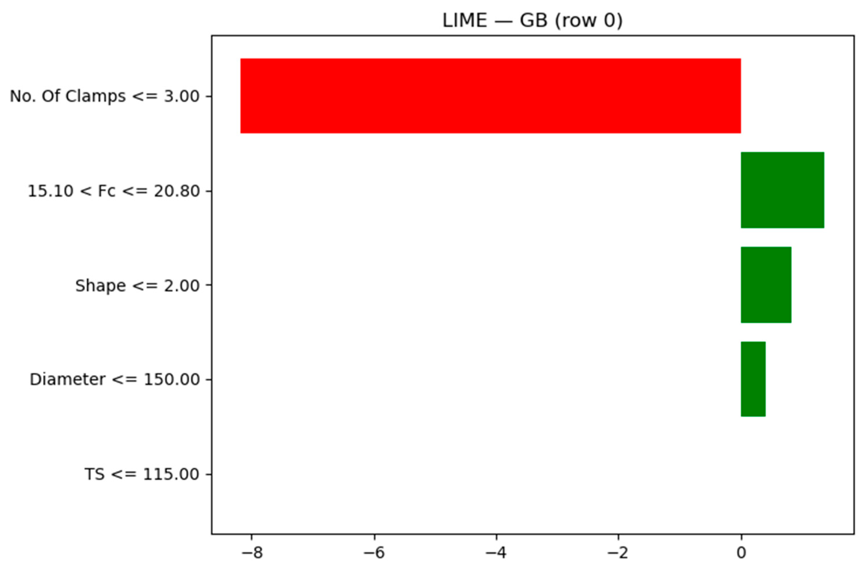
In the analysis presented in Figure 16, we delve into the Local Interpretable Model-Agnostic Explanations (LIME) as applied to the Gradient Boosting (GB) model. This method is instrumental in elucidating the contributions of various features to a specific prediction instance, in this case, row 0. The graphical representation uses horizontal bars to indicate each feature’s influence on the model’s output. Positive contributions are depicted by green bars, suggesting that these features increase the predicted output, whereas red bars illustrate negative contributions, which decrease the expected output. This dual-color coding effectively conveys the impact each feature has in a visually intuitive manner.

A notable observation from the analysis is that the feature “No. of Clamps ≤ 3.00” carries a significant negative weight, substantially reducing the model’s predicted value. This insight suggests that having a limited number of clamps is detrimental to the output for this specific instance, indicating potentially critical operational thresholds that should be considered. Conversely, the analysis reveals that the features associated with moderate ranges of Fc (specifically, 15.10 < Fc ≤ 20.80), Shape ≤ 2.00, Diameter ≤ 150.00, and TS ≤ 115.00 all have positive contributions, although their influence on the model’s output is comparatively lesser than that of the number of clamps. This highlights the relative importance of these geometric and material parameters, which, while supportive, do not carry as much weight as the number of clamps in driving the model’s decision for this instance.

Overall, the findings emphasize that in the given instance of the dataset, the number of clamps is the most critical factor influencing the model’s prediction. In contrast, the material and geometric parameters play a supportive role, contributing positively but to a lesser extent. This analysis provides valuable insights into the feature dynamics at play within the GB model, guiding potential adjustments and considerations for operational practices in relevant applications.

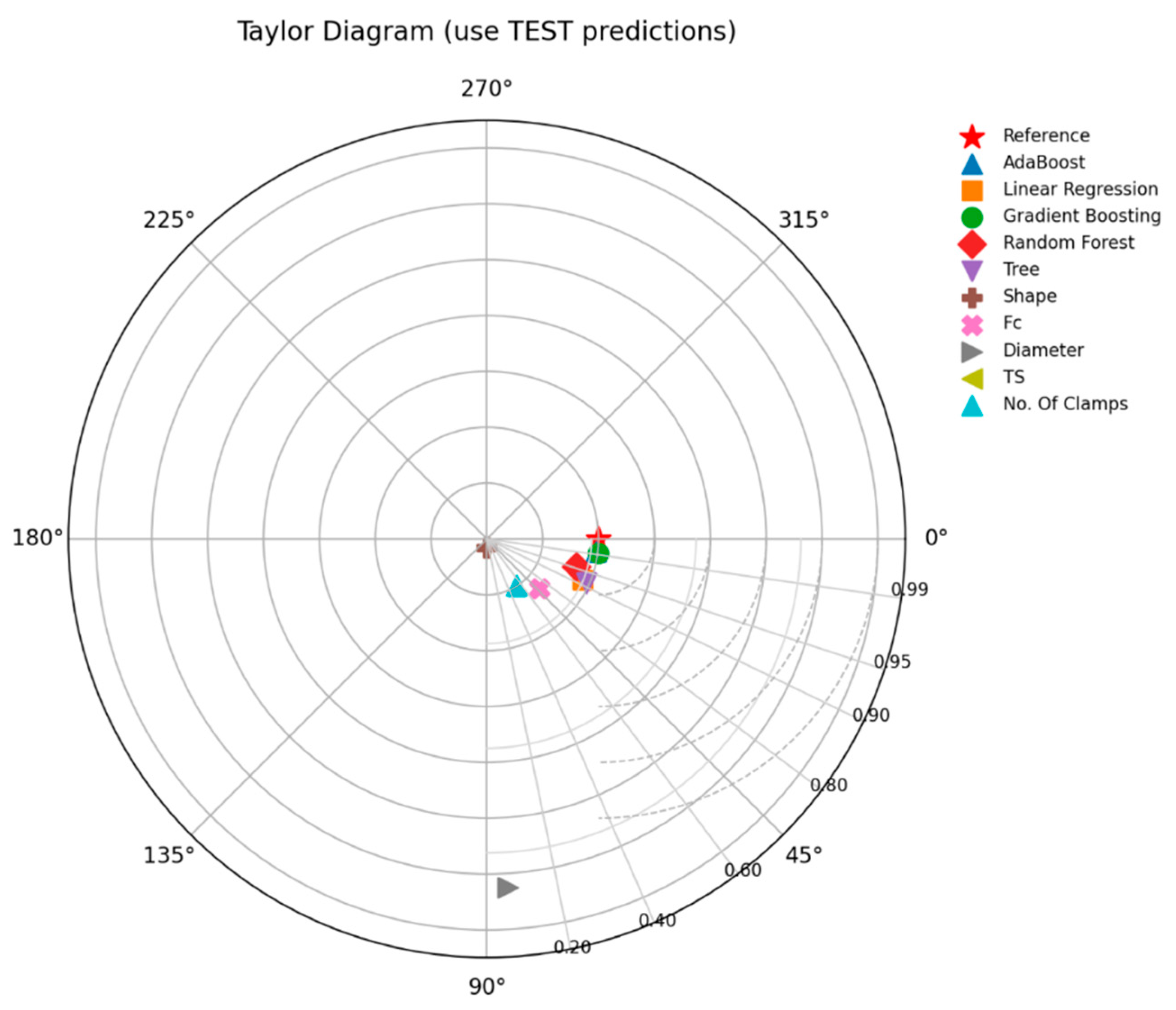
Figure 17 showcases a Taylor Diagram, a sophisticated visual tool that conveys the statistical performance of various predictive models alongside key influencing parameters in relation to reference data derived from test predictions. This diagram effectively integrates three critical measures of model accuracy: the correlation coefficient, standard deviation, and centered root mean square error (RMSE). Plotting these metrics for each model allows for a clear and concise comparison of their reliability and consistency. At the center of the diagram is a distinctive red star representing the observed data, serving as a benchmark for evaluation. Surrounding this reference point, various markers illustrate the performance of different models, including AdaBoost, Linear Regression, Gradient Boosting, and Random Forest, as well as specific parameters such as shape, Fc, diameter, and the number of clamps.

Models that are positioned closer to the reference point indicate a higher level of predictive accuracy. At the same time, those lying along the correlation arc near unity demonstrate strong agreement with the observations. This proximity not only underscores the robustness of the models but also highlights their effectiveness in capturing the nuances of the dataset, making them highly reliable for future predictive tasks.

6. Conclusions

This research presents a comprehensive investigation into the confined compressive strength (Fcc) of different column geometries under varying confinement conditions. The results demonstrate that the circular columns exhibit the highest Fcc values, significantly outperforming both square and rectangular configurations. The study establishes a robust relationship between the number of clamps and Fcc, with increased confinement leading to a notable increase in strength.

Machine learning techniques were used to predict Fcc from various structural parameters. Among the models evaluated, AdaBoost and Gradient Boosting emerged as the most effective, achieving R-squared values of 0.99 and 0.98, respectively. These ensemble methods highlighted the importance of employing multiple models to capture the inherent complexities and interactions within the dataset.

Data visualization techniques, including REC and SHAP values, provided valuable insights into model performance and feature importance. The findings highlight that factors such as the number of clamps and the geometric configurations play critical roles in determining the columns’ compressive strength. The use of LIME further elucidated the complex interplay of features on individual predictions, revealing critical operational thresholds that can guide design choices. Overall, the study underscores the potential for machine learning approaches to enhance predictive modeling in civil engineering applications. The insights gained can help optimize structural designs, ensuring safety and efficiency in construction. Future research could explore applying these models to additional structural shapes and confinement methods, contributing to a more comprehensive understanding of material behavior under varying loading conditions.

References

1. Thomas, C.; Setién, J.; Polanco, J.A.; Alaejos, P.; Juan, M.S. Durability of recycled aggregate concrete. Constr. Build. Mater. 2013, 40, 1054–1065. [Google Scholar] [CrossRef] [Scilit]
2. Pedro, D.; De Brito, J.; Evangelista, L. Durability performance of high-performance concrete made with recycled aggregates, fly ash and densified silica fume. Cem. Concr. Compos. 2018, 93, 63–74. [Google Scholar] [CrossRef] [Scilit]
3. Supit, S.W.M.; Shaikh, F.U.A. Durability properties of high volume fly ash concrete containing nano-silica. Mater. Struct. 2015, 48, 2431–2445. [Google Scholar] [CrossRef] [Scilit]
4. Poon, C.S.; Shui, Z.H.; Lam, L. Effect of microstructure of ITZ on compressive strength of concrete prepared with recycled aggregates. Constr. Build. Mater. 2004, 18, 461–468. [Google Scholar] [CrossRef] [Scilit]
5. Meng, T.; Zhang, J.; Wei, H.; Shen, J. Effect of nano-strengthening on the properties and microstructure of recycled concrete. Nanotechnol. Rev. 2020, 9, 79–92. [Google Scholar] [CrossRef] [Scilit]
6. Wang, L.; Zhou, S.; Shi, Y.; Tang, S.; Chen, E. Effect of silica fume and PVA fiber on the abrasion resistance and volume stability of concrete. Compos. Part B Eng. 2017, 130, 28–37. [Google Scholar] [CrossRef] [Scilit]
7. Nematzadeh, M.; Fallah-Valukolaee, S. Effectiveness of fibers and binders in highstrength concrete under chemical corrosion. Struct. Eng. Mech. Int. J. 2017, 64, 243–257. [Google Scholar]
8. Tabsh, S.W.; Abdelfatah, A.S. Influence of recycled concrete aggregates on strength properties of concrete. Constr. Build Mater. 2009, 23, 1163–1167. [Google Scholar] [CrossRef] [Scilit]
9. Saingam, P.; Chatveera, B.; Promsawat, P.; Hussain, Q.; Nawaz, A.; Makul, N.; Sua-Iam, G. Synergizing Portland Cement, high-volume fly ash and calcined calcium carbonate in producing self-compacting concrete: A comprehensive investigation of rheological, mechanical, and microstructural properties. Case Stud. Constr. Mater. 2024, 21. [Google Scholar] [CrossRef] [Scilit]
10. Padmini, A.; Ramamurthy, K.; Mathews, M. Influence of parent concrete on the properties of recycled aggregate concrete. Constr. Build. Mater. 2009, 23, 829–836. [Google Scholar] [CrossRef] [Scilit]
11. Smarzewski, P. Influence of silica fume on mechanical and fracture properties of high performance concrete. Procedia Struct. Integr. 2019, 17, 5–12. [Google Scholar] [CrossRef] [Scilit]
12. Li, H.; Dong, L.; Jiang, Z.; Yang, X.; Yang, Z. Study on utilization of red brick waste powder in the production of cement-based red decorative plaster for walls. J. Clean. Prod. 2016, 133, 1017–1026. [Google Scholar] [CrossRef] [Scilit]
13. Iffat, S. The characteristics of brick aggregate concrete on a basis of dry density and durability. Malays. J. Civ. Eng. 2016, 28, 1. [Google Scholar] [CrossRef] [Scilit]
14. Juan, M.S.; Gutiérrez, P.A. Study on the influence of attached mortar content on the properties of recycled concrete aggregate. Constr. Build. Mater. 2009, 23, 872–877. [Google Scholar] [CrossRef] [Scilit]
15. Zhu, L.; Zhu, Z. Reuse of Clay Brick Waste in Mortar and Concrete. Adv. Mater. Sci. Eng. 2020, 2020, 6326178. [Google Scholar] [CrossRef] [Scilit]
16. Ahmad, S.; Umar, A. Rheological and mechanical properties of self-compacting concrete with glass and polyvinyl alcohol fibres. J. Build. Eng. 2018, 17, 65–74. [Google Scholar] [CrossRef] [Scilit]
17. Rodsin, K.; Hussain, Q.; Joyklad, P.; Nawaz, A.; Fazliani, H. Seismic strengthening of nonductile bridge piers using low-cost glass fiber polymers. Bull. Pol. Acad. Sci. Tech. Sci. 2020, 68, 6. [Google Scholar] [CrossRef] [Scilit]
18. RILEM Recommendation. Specifications for concrete with recycled aggregates. Mater. Struct. 1994, 27, 557–559. [CrossRef] [Scilit]
19. Konno, K.; Sato, Y. Propriety of recycled aggregate concrete column encased by steel tube subjected to axial compression. Trans. Concr. Inst. 1997, 19, 231–238. [Google Scholar]
20. Zhang, P.; Gao, Z.; Wang, J.; Guo, J.; Ling, Y. Properties of fresh and hardened fly ash/slag based geopolymer concrete: A review. J. Clean. Prod. 2020, 270, 122389. [Google Scholar] [CrossRef] [Scilit]
21. Tibshirani, R. Regression shrinkage and selection via the lasso: A retrospective. J. R. Stat. Soc. Ser. B Stat. Methodol. 2011, 73, 273–282. [Google Scholar] [CrossRef] [Scilit]
22. Ahmad, A.; Farooq, F.; Niewiadomski, P.; Ostrowski, K.; Akbar, A.; Aslam, F.; Alyousef, R. Prediction of compressive strength of fly ash based concrete using individual and ensemble algorithm. Materials 2021, 14, 794. [Google Scholar] [CrossRef] [Scilit]
23. Khademi, F.; Akbari, M.; Jamal, S.M. Prediction of compressive strength of concrete by data-driven models. i-Manag. J. Civ. Eng. 2015, 5, 16–23. [Google Scholar] [CrossRef] [Scilit]
24. Fengying, W. Preliminary research on behaviour of recycled aggregate concrete-filled steel stub columns. J. Fuzhou Univ. 2005, 33, 209–212. [Google Scholar]
25. Azunna, S.U.; Ogar, J.O. Characteristic properties of concrete with recycled burnt bricks as coarse aggregates replacement. Comput. Eng. Phys. Model. 2021, 4, 56–72. [Google Scholar]
26. Ondova, M.; Sicakova, A. Evaluation of the Influence of Specific Surface Treatments of RBA on a Set of Properties of Concrete. Materials 2016, 9, 156. [Google Scholar] [CrossRef] [Scilit] [PubMed]
27. Bazaz, J.B.; Khayati, M.; Akrami, N. Performance of concrete produced with crushed bricks as the coarse and fine aggregate. In The Geological Society of London; Citeseer: State College, PA, USA, 2006; Volume 10. [Google Scholar]
28. Yan, B.; Huang, L.; Yan, L.; Gao, C.; Kasal, B. Behavior of flax FRP tube encased recycled aggregate concrete with clay brick aggregate. Constr. Build. Mater. 2017, 136, 265–276. [Google Scholar] [CrossRef] [Scilit]
29. Gao, C.; Huang, L.; Yan, L.; Kasal, B.; Li, W. Behavior of glass and carbon FRP tube encased recycled aggregate concrete with recycled clay brick aggregate. Compos. Struct. 2016, 155, 245–254. [Google Scholar] [CrossRef] [Scilit]
30. Jiang, T.; Wang, X.M.; Zhang, W.P.; Chen, G.M.; Lin, Z.H. Behavior of FRP-Confined recycled brick aggregate concrete under monotonic compression. J. Compos. Constr. 2020, 24, 04020067. [Google Scholar] [CrossRef] [Scilit]
31. Han, Q.; Yuan, W.Y.; Ozbakkaloglu, T.; Bai, Y.L.; Du, X.L. Compressive behavior for recycled aggregate concrete confined with recycled polyethylene naphthalate/terephthalate composites. Constr. Build. Mater. 2020, 261, 120498. [Google Scholar] [CrossRef] [Scilit]
32. Yang, Y.F.; Han, L.H.; Wu, X. Concrete shrinkage and creep in recycled aggregate concrete-filled steel tubes. Adv. Struct. Eng. 2008, 11, 383–396. [Google Scholar] [CrossRef] [Scilit]
33. Rodsin, K. Confinement effects of glass FRP on circular concrete columns made with crushed fired clay bricks as coarse aggregates. Case Stud. Constr. Mater. 2021, 15, 00609. [Google Scholar] [CrossRef] [Scilit]
34. Atiki, E.; Khechai, A.; Taallah, B.; Feia, S.; Almeasar, K.S.; Guettala, A.; Canpolat, O. Assessment of flexural behavior of compressed earth blocks using digital image correlation technique: Effect of different types of date palm fibers. Eur. J. Environ. Civ. Eng. 2024, 28, 1208–1229. [Google Scholar] [CrossRef] [Scilit]
35. Mousavi, S.M.; Aminian, P.; Gandomi, A.H.; Alavi, A.H.; Bolandi, H. A new predictive model for compressive strength of HPC using gene expression programming. Adv. Eng. Softw. 2012, 45, 105–114. [Google Scholar] [CrossRef] [Scilit]
36. Munir, M.J.; Kazmi, S.M.S.; Wu, Y.F.; Lin, X. Axial stress-strain performance of steel spiral confined acetic acid immersed and mechanically rubbed recycled aggregate concrete. J. Build. Eng. 2021, 34, 101891. [Google Scholar] [CrossRef] [Scilit]
37. Suparp, S.; Ali, N.; Al Zand, A.W.; Chaiyasarn, K.; Rashid, M.U.; Yooprasertchai, E.; Hussain, Q.; Joyklad, P. Axial Load Enhancement of Lightweight Aggregate Concrete (LAC) Using Environmentally Sustainable Composites. Buildings 2022, 12, 851. [Google Scholar] [CrossRef] [Scilit]
38. Xiong, Z.; Wei, W.; Liu, F.; Cui, C.; Li, L.; Zou, R.; Zeng, Y. Bond behaviour of recycled aggregate concrete with basalt fibre-reinforced polymer bars. Compos. Struct. 2021, 256, 113078. [Google Scholar] [CrossRef] [Scilit]
39. Saingam, P.; Hussain, Q.; Sua-Iam, G.; Nawaz, A.; Ejaz, A. Hemp Fiber-Reinforced Polymers Composite Jacketing Technique for Sustainable and Environment-Friendly Concrete. Polymers 2024, 16, 1774. [Google Scholar] [CrossRef] [Scilit] [PubMed]
40. Yang, J.; Du, Q.; Bao, Y. Concrete with recycled concrete aggregate and crushed clay bricks. Constr. Build. Mater. 2011, 25, 1935–1945. [Google Scholar] [CrossRef] [Scilit]
41. Hussain, Q.; Ruangrassamee, A.; Tangtermsirikul, S.; Joyklad, P.; Wijeyewickrema, A.C. Low-cost fiber rope reinforced polymer (FRRP) confinement of square columns with different corner radii. Buildings 2021, 11, 355. [Google Scholar] [CrossRef] [Scilit]
42. Iskander, M.G.; Hassan, M. State of the Practice Review in FRP Composite Piling. J. Compos. Constr. 1998, 2, 116–120. [Google Scholar] [CrossRef] [Scilit]
43. Peng, L.; Miao, X.; Zhu, J.-X.; Zhang, M.-Q.; Zheng, X.-Q.; Li, H.-Y.; Wang, Y.; Jiang, X.; Huang, B.-T. Hybrid machine learning and multi-objective optimization for intelligent design of green and low-carbon concrete. Sustain. Mater. Technol. 2025, 45, e01605. [Google Scholar] [CrossRef] [Scilit]
44. Farooq, F.; Amin, M.N.; Khan, K.; Sadiq, M.R.; Javed, M.F.; Aslam, F.; Alyousef, R. A comparative study of random forest and genetic engineering programming for the prediction of compressive strength of high strength concrete (HSC). Appl. Sci. 2020, 10, 7330. [Google Scholar] [CrossRef] [Scilit]
45. Armaghani, D.J.; Asteris, P.G. A comparative study of ANN and ANFIS models for the prediction of cement-based mortar materials compressive strength. Neural Comput. Appl. 2021, 33, 4501–4532. [Google Scholar] [CrossRef] [Scilit]
46. Freund, Y.; Schapire, R.E. A decision-theoretic generalization of on-line learning and an application to boosting. J. Comput. Syst. Sci. 1997, 55, 119–139. [Google Scholar] [CrossRef] [Scilit]
47. Feng, D.-C.; Liu, Z.T.; Wang, X.D.; Chen, Y.; Chang, J.Q.; Wei, D.F.; Jiang, Z.M. Machine learning-based compressive strength prediction for concrete: An adaptive boosting approach. Constr. Build. Mater. 2020, 230, 117000. [Google Scholar] [CrossRef] [Scilit]
48. Behnood, A.; Golafshani, E.M. Machine learning study of the mechanical properties of concretes containing waste foundry sand. Constr. Build. Mater. 2020, 243, 118152. [Google Scholar] [CrossRef] [Scilit]
49. Ahmad, A.; Lagaros, N.D.; Cotsovos, D.M. Neural Network-Based Prediction: The Case of Reinforced Concrete Members under Simple and Complex Loading. Appl. Sci. 2021, 11, 4975. [Google Scholar] [CrossRef] [Scilit]
50. Le-Nguyen, K.; Minh, Q.C.; Ahmad, A.; Ho, L.S. Development of deep neural network model to predict the compressive strength of FRCM confined columns. Front. Struct. Civ. Eng. 2022, 16, 1213–1232. [Google Scholar] [CrossRef] [Scilit]
51. Al-Sayegh, A.T.; Mahmoudabadi, N.S.; Shabbir, F.; Alkandari, F.J.; Saghir, S.; Ahmad, A. Prediction of load-bearing capacity of RC columns (CWA) using Artificial Neural Networks (ANN) trained on a hybrid experimental database HEXP. J. Eng. Res. 2025, 13, 3007–3025. [Google Scholar] [CrossRef] [Scilit]
52. Ahmad, A.; Cotsovos, D.M. Reliability analysis of models for predicting T-beam response at ultimate limit response. Proc. Inst. Civ. Eng.-Struct. Build. 2023, 176, 28–50. [Google Scholar] [CrossRef] [Scilit]
53. Ahmad, A.; Aljuhni, A.; Arshid, U.; Elchalakani, M.; Abed, F. Prediction of columns with GFRP bars through Artificial Neural Network and ABAQUS. In Structures; Elsevier: Amsterdam, The Netherlands, 2022; pp. 247–255. [Google Scholar]
54. Ahmad, A.; Arshid, M.U.; Mahmood, T.; Ahmad, N.; Waheed, A.; Safdar, S.S. Knowledge-Based Prediction of Load-Carrying Capacity of RC Flat Slab through Neural Network and FEM. Math. Probl. Eng. 2021, 2021, 18. [Google Scholar] [CrossRef] [Scilit]
55. Mashhadban, H.; Kutanaei, S.S.; Sayarinejad, M.A. Prediction and modeling of mechanical properties in fiber reinforced self-compacting concrete using particle swarm optimization algorithm and artificial neural network. Constr. Build. Mater. 2016, 119, 277–287. [Google Scholar] [CrossRef] [Scilit]
56. Cao, Y.; Miao, Q.; Liu, J.C.; Gao, L. Advance and prospects of AdaBoost algorithm. Acta Autom. Sin. 2013, 39, 745–758. [Google Scholar] [CrossRef] [Scilit]
57. Dev, V.A.; Eden, M.R. Gradient boosted decision trees for lithology classification. Comput. Aided Chem. Eng. 2019, 47, 113–118. [Google Scholar]
58. Syam, N.; Kaul, R. Random forest, bagging, and boosting of decision trees. In Machine Learning and Artificial Intelligence in Marketing and Sales: Essential Reference for Practitioners and Data Scientists; Emerald Publishing Limited: Leeds, UK, 2021; pp. 139–182. [Google Scholar]
59. Asselman, A.; Khaldi, M.; Aammou, S. Enhancing the prediction of student performance based on the machine learning XGBoost algorithm. Interact. Learn. Environ. 2023, 31, 3360–3379. [Google Scholar] [CrossRef] [Scilit]
60. Chen, T.; Guestrin, C. Xgboost: A scalable tree boosting system. In KDD’16: Proceedings of the 22nd ACM SIGKDD International Conference on Knowledge Discovery and Data Mining; Association for Computing Machinery: New York, NY, USA, 2016; pp. 785–794. [Google Scholar]
61. Asteris, P.G.; Apostolopoulou, M.; Skentou, A.D.; Moropoulou, A. Application of artificial neural networks for the prediction of the compressive strength of cementbased mortars. Comput. Concr. 2019, 24, 329–345. [Google Scholar]
62. Zhang, P.; Liu, C.; Li, Q. Application of gray relational analysis for chloride permeability and freeze-thaw resistance of high-performance concrete containing nanoparticles. J. Mater. Civ. Eng. 2011, 23, 1760–1763. [Google Scholar] [CrossRef] [Scilit]
63. ASTM C140/C140M-22b; Standard Test Methods for Sampling and Testing Concrete Masonry Units and Related Units. ASTM International: West Conshohocken, PA, USA, 2022.
64. C943-17 ASTM; Standard Practice for Making Test Cylinders and Prisms for Determining Strength and Density of Preplaced-Aggregate Concrete in the Laboratory. ASTM International: West Conshohocken, PA, USA, 2017.
Figure 1. Details of specimens (units in mm).
Buildings 16 00851 g001
Figure 2. Parameters description between diameter and Fcc.
Buildings 16 00851 g002
Figure 3. Parameters description between Fc and Fcc.
Buildings 16 00851 g003
Figure 4. Parameters description between the number of clamps and Fcc.
Buildings 16 00851 g004
Figure 5. Parameters description between shape and Fcc.
Buildings 16 00851 g005
Figure 6. Correlation heatmap of input parameters and target variable.
Buildings 16 00851 g006
Figure 7. Flow Chart.
Buildings 16 00851 g007
Figure 8. Model Diagnostics for Linear Regression.
Buildings 16 00851 g008
Figure 9. Model Diagnostics for Decision Tree.
Buildings 16 00851 g009
Figure 10. Model Diagnostics for Random Forest.
Buildings 16 00851 g010
Figure 11. Model Diagnostics for AdaBoost.
Buildings 16 00851 g011
Figure 12. Model Diagnostics for Gradient Boosting.
Buildings 16 00851 g012
Figure 13. REC for Training Data.
Buildings 16 00851 g013
Figure 14. REC for Testing Data.
Buildings 16 00851 g014
Figure 15. SHAP (SHapley Additive exPlanations) summary plot.
Buildings 16 00851 g015
Figure 16. Local Interpretable Model-Agnostic Explanations (LIME).
Buildings 16 00851 g016
Figure 17. Tylor Diagram for the studied Models.
Buildings 16 00851 g017