Prediction of the Extreme Dynamic Amplification Factor Based on Bayesian Peaks-over-Threshold–Generalized Pareto Distribution Method and Random Traffic–Bridge Interaction

Abstract

The accurate prediction of extreme dynamic amplification factor (DAF) values is significantly important to ensure a long-term safety assessment of bridges under stochastic vehicular loading. However, predicting extreme DAFs is challenging due to traffic randomness, road roughness variability, and nonlinear vehicle–bridge interaction (VBI) effects. This study presents an integrated framework for extreme DAF prediction for simply supported bridges by combining stochastic traffic–bridge interaction simulations with Bayesian updating and a Peaks-Over-Threshold–Generalized Pareto Distribution (POT–GPD) model. A coupled VBI model is developed, incorporating cellular automaton-based traffic flow, multi-axle nonlinear vehicle dynamics, finite-element bridge modeling, and stochastic road roughness profiles. A new DAF definition based on dynamic displacement difference is proposed to better represent dynamic effects. DAF samples obtained from VBI simulations under different road roughness levels are analyzed using the POT method, with GPD parameters estimated through maximum likelihood and Bayesian inference. Extreme DAFs corresponding to different return periods are then determined. The results indicate that extreme DAF values increase with worsening road roughness and longer return periods and that the Bayesian POT–GPD approach effectively captures tail behavior while providing reliable uncertainty quantification for extreme DAF prediction.

1. Introduction

Bridges are critical components of transportation infrastructures. Their safety and longevity have a significant role in ensuring efficient accessibility and interconnectivity across regions. Throughout their service life, bridges are subjected to complex dynamic loading conditions, primarily caused by traffic. The dynamic interaction forces between the bridge and the moving vehicles, commonly referred to as vehicle–bridge interaction (VBI), induce a dynamic response that is often significantly greater than those estimated by static loading.

To account for these amplified dynamic effects in the design, the DAF is commonly employed. Therefore, the accurate prediction of DAF, particularly their extreme values, is critical for guaranteeing the bridges’ structural safety and developing rational design standards. However, the randomness of traffic flows, the effect of road irregularities, and the complexity of the VBI system make the precise estimation of extreme DAF values a considerable challenge. O’Brien et al. [1] developed a methodology to predict lifetime DAF for various concrete bridges. The estimated DAF was consistently lower than the recommended values in design codes. Similarly, Caprani et al. [2] utilized extreme value theory (EVT) to estimate the DAF based on site-specific traffic loads, and the estimated DAFs was significantly lower than the values specified in design codes. Conversely, Cai et al. [3] employed an EVT to predict extreme responses in prestressed concrete bridges using short-term monitoring data, and the results demonstrate that DAF values exceed those recommended in the AASHTO specifications. Jafarian Kafshgarkolaei et al. [4] investigated extreme dynamic responses of beam-type structures under various loading conditions. Bagheri et al. [5] also examined extreme events in RC structures under dynamic loading, demonstrating significant displacement amplification relevant to the interpretation of extreme DAF.

However, existing research on the prediction of DAF remains relatively limited, with most available studies focusing on deterministic or simplified probabilistic approaches that do not fully capture the stochastic nature of traffic–bridge interactions. Furthermore, these studies commonly rely on traditional extreme value or empirical methods, without considering the more recent and powerful approaches capable of accurately representing the tail behavior of extreme responses. These show the need for more statistically reliable approaches to characterize the extreme tail behavior of DAF.

Over the past few years, more advanced methodologies have been developed based on the EVT to quantify the estimation of extreme bridge dynamic responses based on traffic data. In particular, the POT method associated with GPD has been extensively employed to effectively model the extreme dynamic effects on bridges, as it provides a significant statistical foundation for clearly understanding the probabilistic nature of rare events. Zhou et al. [6] employed a GPD method for estimating maximum bridge response using traffic data, and the results demonstrate the method’s effectiveness in performing extreme value analysis. Adam et al. [7] proposed a slice sampler algorithm based on the GPD model for multiple simulated datasets, and a comparable performance was obtained with other methods. Liu et al. [8] used WIM data to estimate the service life for different span bridges using GPD, showing the applicability of the model performance for various bridge types. Xu et al. [9] performed an extreme value analysis using a GPD model to study the influence of temperature on arch bridges. Deng et al. [10] developed an extreme value assessment for suspension bridges by integrating POT with GPD, thereby demonstrating the ability of the GPD for structural response extremes. Zhou et al. [11] used a GPD to model extreme lane load effects based on short-term traffic data from a simply supported bridge. The POT–GPD method provides better estimation under small sample data. These studies simultaneously show the capacity of the GPD model for determining the statistical nature of extreme load effects of bridges. However, most of them are highly dependent on the classical frequentist estimation techniques, which may provide inaccurate uncertainty predictions for parameters, especially when dealing with limited sample data.

To address these challenges, Bayesian inference has been introduced in bridge loads modeling and reliability assessment [12], as it provides a powerful probabilistic approach for evaluating parameter estimation and uncertainty quantification in extreme value analysis. Jacinto et al. [13] performed a structural assessment of existing bridges using the Bayesian method for bridge monitoring data. Yu et al. [14] applied a Bayesian method to estimate the non-stationary extreme traffic load effects on bridges. A better result was found for the bridge performance assessment. Ni et al. [15] applied a Bayesian method to study the effect of extreme loads on cable-stayed bridge expansion joints. Rizqiansyah et al. [16] utilized a hierarchical Bayesian modeling to estimate service life for multiple bridges based on extreme traffic load data. A significant reduction in prediction uncertainties was obtained. Yan et al. [17] employed a Bayesian inference to predict the extreme dynamic effect on RC bridges. The updated models demonstrated close agreement with the measurement data. Wang et al. [18] proposed a Bayesian probabilistic method to predict the extreme load value of a cable-stayed bridge from WIM data. The method’s performance was compared for multiple vehicle loading scenarios. Li et al. [19] employed a Bayesian deep learning approach to estimate the dynamic vibration response of bridges based on the VBI data from railway bridges. The result shows the Bayesian method combined with VBI data provides a better estimate under limited sample data. O’Brien et al. [20] used a Bayesian approach to determine bridge damage and road profile based on the acceleration of passing vehicles. Pei et al. [21] developed Bayesian Inference approach to study the temperature effects on steel bridges. Luo et al. [22] proposed a predictive framework using GEV distribution and Bayesian updating on RC bridges using VBI analysis. It proved that Bayesian updating can effectively predict the dynamic responses of RC bridges.

These works confirm the suitability of the Bayesian approach for handling parameter uncertainties under limited samples. Furthermore, some studies combined Bayesian inference with the GPD model to establish a unified Bayesian POT–GPD framework for more accurate extreme value prediction. Gao et al. [23] employed a Bayesian approach with the GPD to determine the extreme traffic effects on arch bridge suspenders, showing that the integration of Bayesian estimation significantly improves predictions. Xu et al. [24] proposed a Bayesian approach with GPD to estimate extreme load on a cable-stayed bridge using limited data. Mendoza et al. [25] applied the Bayesian method with EVT to assess bridge criticality using limited samples from WIM data. The predicted extreme load effects were subsequently compared with design codes.

Despite these achievements, a significant gap remains in the specific domain of extreme DAF value prediction. To overcome these limitations, in this study, a Bayesian POT-GPD framework is developed to estimate the DAFs of bridges under random traffic flow. This framework incorporates (1) a coupled traffic–bridge interaction (VBI) dynamic simulation using a cellular automaton (CA) traffic flow model to generate random, realistic vehicular movement across varying surface roughness levels; (2) follows an innovative approach to calculate the DAF based on the dynamic displacement difference that captures time-dependent amplification effects throughout the entire simulation; and (3) the Bayesian updating method combined with Markov Chain Monte Carlo (MCMC) sampling to enhance the posterior distributions of GPD parameters under limited sample data was employed. The extreme DAFs for different return periods under different road roughness are further discussed.

2. DAF Based on Dynamic Displacement Difference in Random Traffic–Bridge Interaction

2.1. Random Traffic Flow Simulation

A random traffic flow and bridge dynamic simulation system provides a computational framework for determining the dynamic responses behavior of bridge structures subjected to stochastic vehicular loading. In previous studies, scholars carried out the dynamic effects of VBI analysis under various traffic flow conditions and bridge systems. For example, Li et al. [26] introduced a time-varying updating technique for coupled VBI analysis, while Zhao et al. [27] studied how fluid viscous dampers influence suspension bridge responses under traffic flow simulation, and Wei et al. [28] proposed a coupling framework for suspension bridges to assess the effects of lane arrangement and traffic flow. Ebrahimzadeh Hassanabadi et al. [29] investigated beam vibration dynamics and proposed an efficient orthonormal polynomial-based formulation for dynamic analysis. Also, Asgari et al. [30] experimentally validated load–capacity relationships with analytical models under combined loading, supporting response-based dynamic assessment.

2.1.1. Single Vehicle Dynamic Model

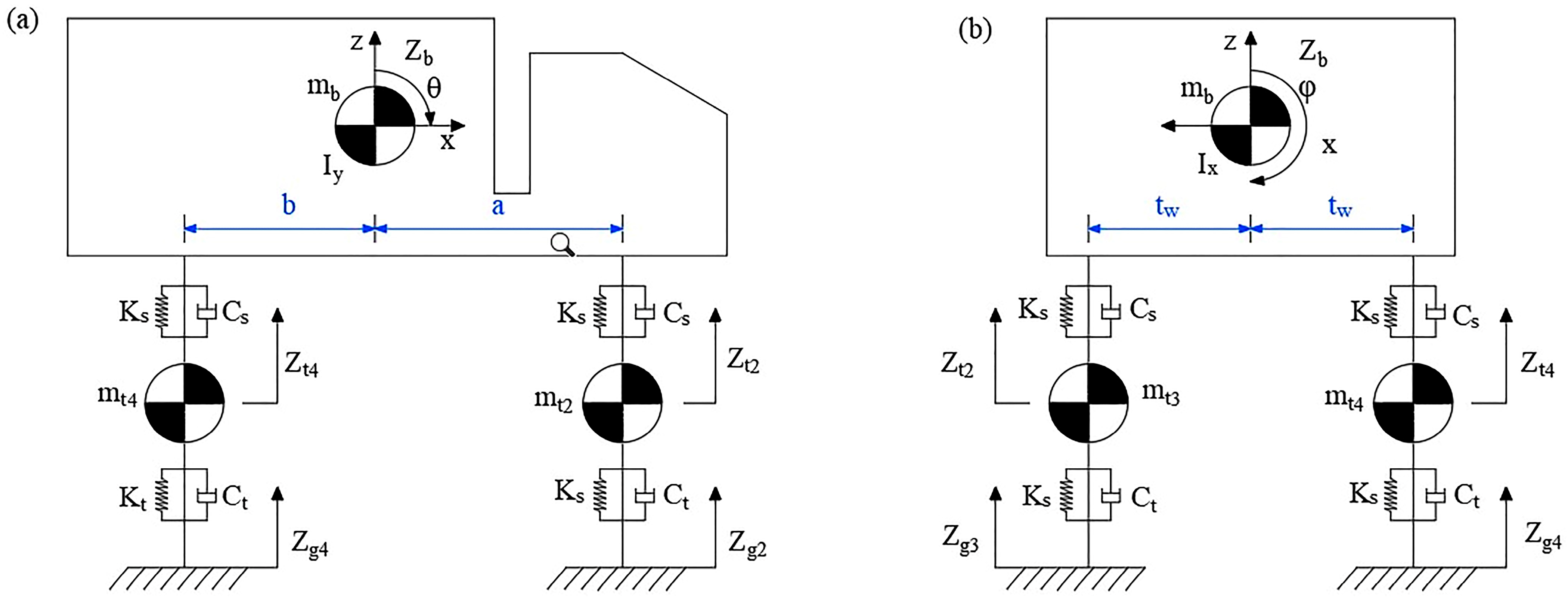
A random traffic flow is composed of several vehicles with different types and properties. Their dynamic behaviors should be fully described and applied to the bridges. For a single vehicle, the dynamic model is represented by rigid bodies and suspension systems. The vehicle body and tires are treated as a rigid body. The suspension system is idealized as spring and damper components that connect the vehicle body with axles. The vehicle tires were modeled considering a linear spring element that accounts for stiffness and damping properties. In fact, the traffic flow consists of various kinds of vehicles with different axle numbers. To simulate random traffic flow, vehicles with two to six axles are considered, corresponding to 7, 9, 11, 13, and 15 degrees of freedom, respectively. As an example, the simplified dynamic model of a two-axle vehicle with seven degrees of freedom is shown in Figure 1. The vehicle body has three degrees of freedom, including the vertical translation, rotation about a horizontal axis, and rotation about the longitudinal axis, which are represented by the vertical displacement $(Z)$, pitch angle $(\theta )$, and roll angle $(\phi )$, respectively. Each tire of the vehicle has an additional vertical displacement degree of freedom $(Z_{t1}, Z_{t2}, Z_{t3}, Z_{t4})$. The dynamic motion equations of a vehicle body and each tire are described as follows [31]:

In the vertical direction of the vehicle body (along the z-axis),

$$m_b{\ddot{Z}}_b=C_s{\displaystyle \sum _{i=1}^4\left({\dot{Z}}_{ti}-{\dot{Z}}_{bi}\right)}-K_s{\displaystyle \sum _{i=1}^4\left(Z_{ti}-Z_{bi}\right)}=0$$

(1)

In the longitudinal direction of the vehicle body (along the x-axis),

$$I_y\ddot{\theta }-b\left[C_s{\displaystyle \sum _{i=1}^4\left(Z_{ti}-Z_{bi}\right)+K_s{\displaystyle \sum _{i=1}^4\left(Z_{ti}-Z_{bi}\right)}}\right]+a\left[C_s{\displaystyle \sum _{i=1}^4\left(Z_{ti}-Z_{bi}\right)+K_s{\displaystyle \sum _{i=1}^4\left(Z_{ti}-Z_{bi}\right)}}\right]-m_{b}hg\theta =0$$

(2)

In the transversal direction of the vehicle body (along the y-axis),

$$I_x\phi -t_t\left[C_s{\left(-1\right)}^{i+1}{\displaystyle \sum _{i=1}^4\left(Z_{ti}-Z_{bi}\right)}+K_s{\left(-1\right)}^{i+1}{\displaystyle \sum _{i=1}^4{Z}_{ti}-Z_{bi}}\right]-m_{b}hg\theta =0$$

(3)

In the vertical direction for the four tires,

$$M_{ti}{\ddot{Z}}_{ti}-C_s\left({\dot{Z}}_{bi}-{\dot{Z}}_{ti}\right)-C_t\left({\dot{Z}}_{ri}-{\dot{Z}}_{ti}\right)-K_s\left(Z_{bi}-Z_{ti}\right)-K_t\left(Z_{ri}-Z_{ti}\right)=0, (i=1,2,3,4)$$

(4)

where $m_{ti}$ and $m_b$ denotes the mass of the $i\mathrm{th}$ tire and the vehicle body, respectively; $I_y$ and $I_x$ are the mass moment of inertia about the y- and x-axes. $C_t$, $C_s$ and $K_t$, $K_s$ represent damping and stiffness for the tires and suspension system. $a$ and $b$ denotes the front and rear axles distances from the vehicle’s gravity center. $h$ is the distance from the tires to the vehicle’s gravity center. $\theta$ and $\phi$ denote the rolling displacements of the vehicle about the y- and x-axes. $Z_{ti}$ and $Z_{bi}$ are the vertical displacement of the $i\mathrm{th}$ tire and suspension–body connection point, respectively; $Z_{ri}$ is the road surface elevation at the $i\mathrm{th}$ contact point, including bridge girder deformation.

2.1.2. Random Traffic Flow Method

Traffic flow simulation has a significant impact on the traffic flow–bridge dynamic system, as it provides a realistic representation of vehicular movement across the bridge, ensuring accurate evaluation of dynamic responses. Various techniques have been used to model traffic flow simulations on different types of bridges. Chen and Wu [32] applied the cellular automaton (CA) method to solve traffic loads on bridges, while Chen et al. [33] studied the combined random traffic and bridges dynamic effects of using a CA traffic simulation. Zhu et al. [34] employed a pseudo-excitation technique to study the dynamic coupling effect on the train–track–bridge interaction. Han et al. [35] also employed the CA method to develop a random traffic flow–bridge interaction, which was then used to evaluate the impact factor (IM) of the bridge. However, Chen et al. [36] introduced a probabilistic approach using an undirected graphical model to represent the stochastic distribution of traffic loads on bridges. Wang and Xu [37] utilized WIM data to model traffic flow, incorporating lane-changing rules and vehicle-following behavior on a suspension bridge. Yao et al. [38] adopted a time-division-based Markov model to estimate short-term traffic flow across different time periods. However, the cellular automaton (CA) method remains the most commonly used approach for analyzing random traffic simulations, as was performed by Yin et al. [39].

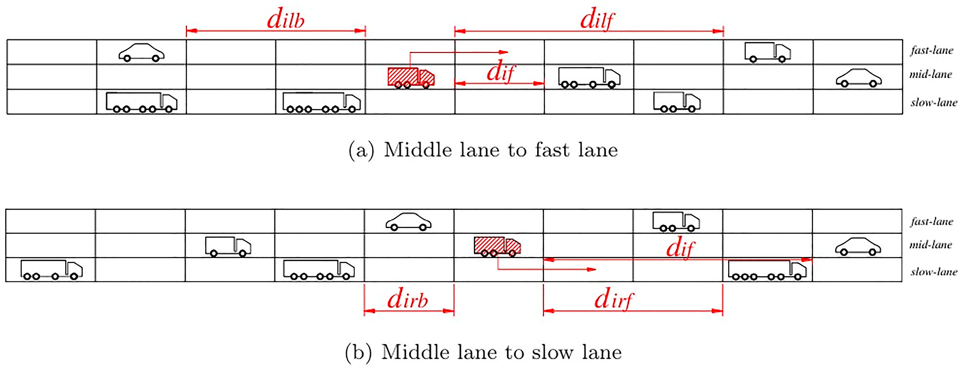
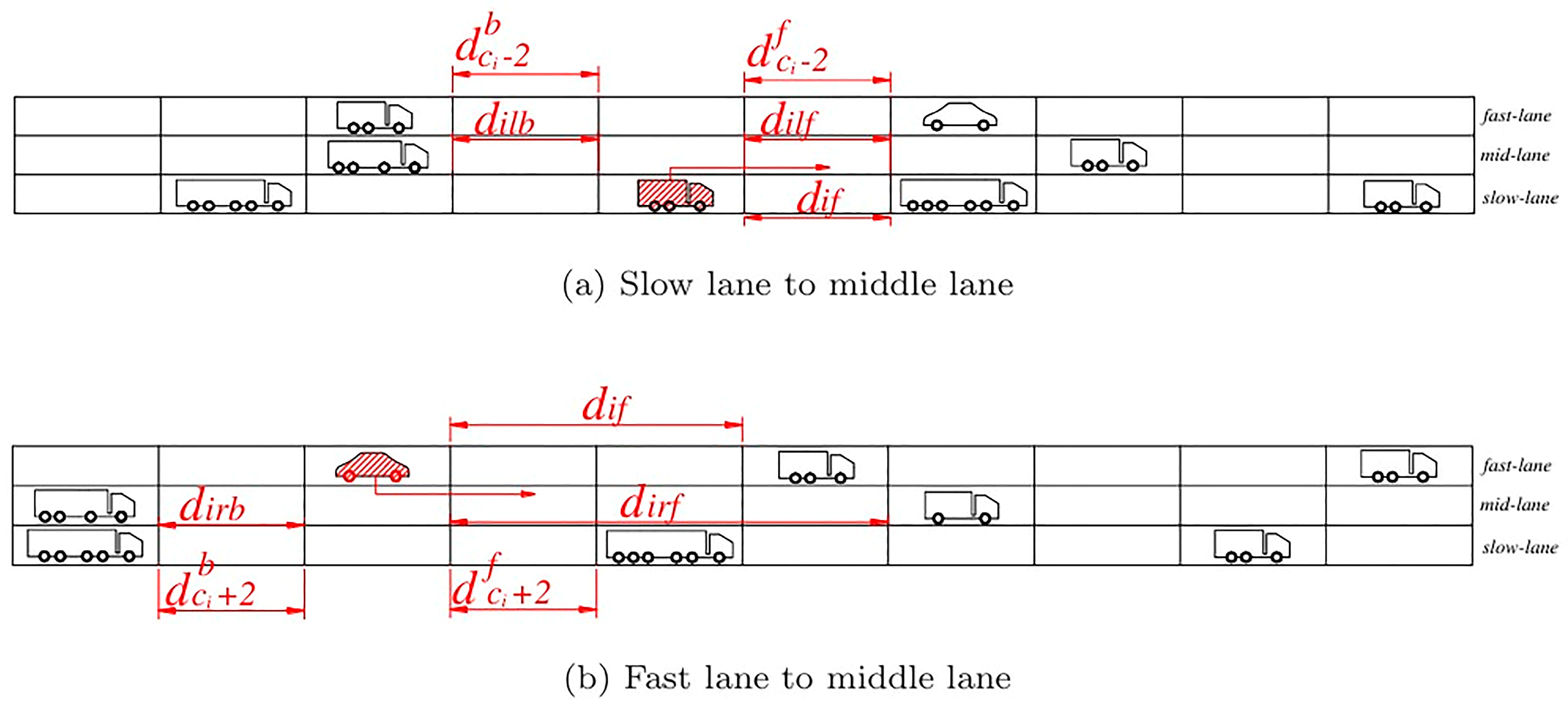
After a thorough review of previous studies and existing methods for random traffic flow simulation, this paper applies the classical CA method to conduct traffic flow on a simply supported bridge, as it provides a realistic random traffic simulation on bridges. In the CA method, the traffic flow–bridge system is proposed, taking into account random traffic, dynamic coupling effects, and the surface irregularity on the bridge. The bridge is modeled as a series of discrete cells; each cell is represented by the small segment on the bridge deck that may be occupied by the vehicle or unoccupied. The time progresses in discrete steps, and the vehicle movement on the bridge follows simple rules based on local iterations, which means the vehicle accelerates if the next cell is not occupied by another vehicle, slows down to avoid the collisions, and randomly brakes to simulate the driver’s behavior. The bridge deck is divided into three lanes: a slow, middle, and fast lane, as shown in Figure 2. Each cell length is 7.5 m. The maximum cell speeds are set to 3 cells/s, 4 cells/s, and 5 cells/s for the slow, middle, and fast lanes, respectively. The cell status updating time interval is 1 s. Also, the positions of the $i\mathrm{th}$ vehicle before changing lanes are shown in Figure 3. Xia et al. [40] and Wang et al. [41].

• The vehicle shifts from middle to slow/fast lanes.

In this case, if $c_i$ is the lane number of the $i\mathrm{th}$ vehicle, the vehicle shifts to the fast lane, as follows:

$$c_i=\left\{\begin{array}{l}{c}_i-1 , if d_{if}<d_{safe}, d_{ilf}>d_{safe}, d_{ilb}>1+{(v_{c_i-1})}_{\max }-\min \left\{v_i+1,{(v_{c_i-1})}_{\max }\right\}, else\\ v_i\end{array}\right.$$

(5)

where $v_i$ is the $i\mathrm{th}$ vehicle speed, ${\left(v_{c_i-1}\right)}_{max}$ is the vehicle speed on the $c_{i }-1$ lane; $d_{if}$ and $d_{safe}$ are unitless distances (actual distance/Lc); and Lc is the cell length.

And the vehicle will shift to the slow lane, as follows:

$$c_i=\left\{\begin{array}{l}{c}_i-1 , if d_{if}<d_{safe}, d_{irf}>d_{safe} , d_{irb}>d_{safe} ,else \\ c_i\end{array}\right.$$

(6)

2.

The vehicles shift from fast/slow lane to middle lane.

The $i\mathrm{th}$ vehicles location before shifting from fast/slow lane to middle lane is shown in Figure 4. The changing possibility is described by

$$c_i=\left\{\begin{array}{l}{c}_i-1 , if d_{if}<d_{safe}, d_{ilf}>d_{safe} , d_{ilb}>1+{(v_{c_i-1})}_{\max }-\min \left\{v_i+1,{(v_{c_i-1})}_{\max }\right\} , \\ \min \left\{{d^b}_{c_i-2}, {d^f}_{c_i-2}\right\} <d_{safe} ,else \\ c_i\end{array}\right.$$

(7)

or

It probably shifts to the middle lane, as follows:

$$c_i=\left\{\begin{array}{l}{c}_i-1 , if d_{if}<d_{safe}, d_{irf}>d_{safe} , d_{irb}>d_{safe}, \min \left\{{d^b}_{c_i+2}, {d^f}_{c_i+2}\right\} <d_{safe} ,else \\ c_i\end{array}\right.$$

(8)

3.

The vehicle’s acceleration and deceleration

If the vehicle speed is below the maximum limit ($v_{c_i}$), the vehicle will accelerate, and the speed $v_i$ is described by

$$c_i=\left\{\begin{array}{l}\min \left\{v_i+1,{(v_{ci})}_{\max }\right\} , if d_{if}<d_{safe}, v_i<{(v_{ci})}_{\max } ,else \\ v_i\end{array}\right.$$

(9)

If the vehicle speed is higher than the maximum limit, it will possibly decelerate, and the resulting speed is defined as

$$c_i=\left\{\begin{array}{l}\min \left\{v_i+1,{(v_{ci})}_{\max }\right\} , if d_{if}<d_{safe}, d_{if}\ge {(v_{ci})}_{\max }-{(v_{ci})}_{\min }\\ {(v_{ci})}_{\max } , if d_{if}<d_{safe}, d_{if}<{(v_{ci})}_{\max }-{(v_{ci})}_{\min }, else\\ v_i\end{array}\right.$$

(10)

4.

The vehicle’s random slowing

Due to road surface and other conditions, the vehicles possibly decelerate randomly, which is described by

$$c_i=\max \left\{v_i-1,{(v_{ci})}_{\min }\right\} v_i>{(v_{c_i})}_{\max }$$

(11)

2.2. Traffic–Bridge Interaction

The bridge is discretized using FE methods to divide the bridge deck into small elements to consider its material and geometrical properties. The bridge equation of motion is described as

$$M_b{\ddot{Z}}_d+C_b{\dot{Z}}_d+K_b{Z}_d=F_v$$

(12)

where ${\ddot{Z}}_d$, ${\dot{Z}}_d$, and $Z_d$ represent the nodal vectors of acceleration, velocity, and displacement, respectively. $M_b$, $C_b$, and $K_b$ represent the global mass, damping, and stiffness matrices, and $F_{vb}$ is the vehicle force vector.

The Rayleigh damping was considered for the FE bridge model. Since the bridge deck surface deteriorates due to construction and environmental factors, the resulting vertical surface irregularities introduce randomness that generates additional dynamic excitation, amplifying the response for the vehicle and bridge. Therefore, it is mandatory to consider the influence of bridge surface irregularities during the VBI analysis. According to Dodds and Robson [42], pavement roughness can be modeled as a stationary Gaussian stochastic process with zero mean and generated by inverse Fourier transform using a power spectral density (PSD) function. The mathematical expression is given by $G(n)=G(n_0){(n/n_0)}^{-w}$, where $G(n)$ denotes the power spectral density of the road elevation, $n$ is the spatial frequency, $n_0$ is the reference spatial frequency, and $w$ is the waviness exponent. In addition, the roughness levels A, B, and C are defined by increasing values of the reference PSD $G(n_0)$, consistent with the ISO 8608 standard [43], representing good, average, and poor road surface conditions, respectively.

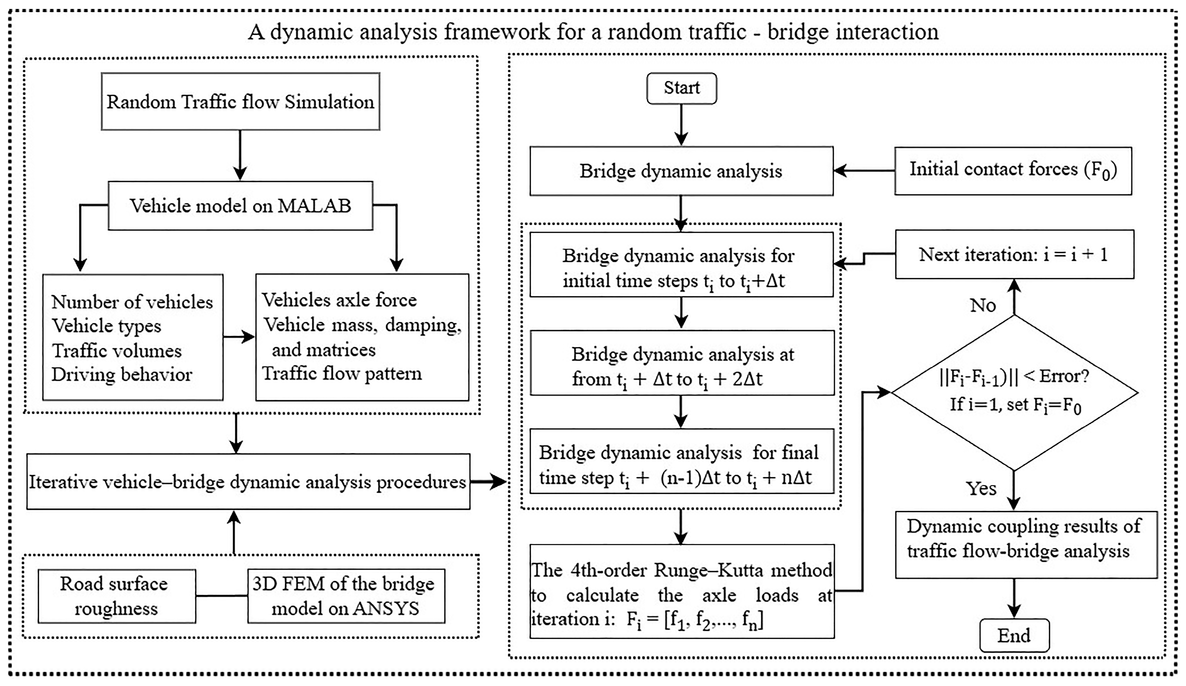
The random traffic–bridge interaction is primarily determined by the VBI forces within the vehicles and bridge. This coupled interaction system is modeled by solving the dynamic equations of the VBI system simultaneously through their interaction forces, Yu et al. [31]. The vehicle dynamic equations for the random traffic flow were computed according to the fourth-order Runge–Katta method. The bridge FEM is developed in the ANSYS software (v2023 R1), and the transient nodal displacements are extracted and combined with road surface roughness as the moving boundary for the vehicles [40]. The solution procedure for the coupled traffic flow–bridge interaction system is described in Figure 5.

2.3. DAF Based on Dynamic Displacement Difference

2.3.1. Definition of DAF

DAF is a crucial parameter in the design and assessment of bridge performances to quantify the dynamic effect, which is caused by moving vehicles on the bridge. In most of the previous studies [44,45] the definition of DAF is given as the ratio of the maximum dynamic response of the bridge (e.g., displacement, internal forces, stress) under moving vehicles to the static response under the same vehicle loading condition, only considering the static effect. For example, considering the displacement-based bridge response, the DAF is defined as

$$DAF={\displaystyle \frac{D_{\max }}{S_{\max }}}$$

(13)

where $D_{\max }$ is the maximum displacement at some specific position of the bridge as the vehicles pass the bridge, which is called maximum dynamic displacement; and $S_{\max }$ represents the maximum static displacement at a certain position.

Although this conventional definition of DAF is commonly utilized in design standards and studies, it shows certain drawbacks. The definition is overly simplistic and does not adequately capture the influence of dynamic effects. It relies exclusively on maximum peak responses that do not occur under the same vehicle conditions, which may not fully account for the incremental differences between the dynamic and static responses throughout the vehicle passage. This problem is even more challenging when a traffic flow involving multiple vehicles is considered. In such cases, the bridge maximum static response arises from specific vehicle configurations, such as multiple vehicles concentrated at midspan. These configurations are entirely different from those that produce the maximum dynamic response. Consequently, conventional DAF definitions are primarily intended for practical engineering design applications, where simplicity and conservatism are emphasized, rather than for a strict mathematical representation of dynamic behavior. Comparing these different cases through a simple ratio may provide an effective estimate of the combined effect of static and dynamic responses, but it may not precisely isolate the amplified dynamic effect. Therefore, this method can significantly underestimate or overestimate the dynamic response of the bridge in terms of both physical interpretability and statistical effectiveness, particularly when used for extreme value prediction.

For the definition of DAF in Equation (13), the dynamic displacement $D$ can be decomposed as the static displacement $S$ and the dynamic displacement difference $\Delta D$. Thus, Equation (13) can be analyzed further as

$$DAF={\displaystyle \frac{{(S+\Delta D)}_{\max }}{S_{\max }}}\le {\displaystyle \frac{S_{\max }+\Delta D_{\max }}{S_{\max }}}=1+{\displaystyle \frac{\Delta D_{\max }}{S_{\max }}}$$

(14)

where $\Delta D_{\max }$ represents the maximum dynamic displacement differences, and ${\mathrm{S}}_{\mathrm{m}\mathrm{a}\mathrm{x}}$ is the maximum static displacement at some position on the bridge.

A new DAF ($DA{F}_N$) based on dynamic displacement difference is then defined as

$$DA{F}_N=1+{\displaystyle \frac{\Delta D_{\max }}{S_{\max }}}$$

(15)

It offers a more physically and mathematically meaningful representation for the bridge’s dynamic response induced by traffic flow–bridge interaction forces. This method clearly integrates the time-dependent displacement variation between dynamic and static responses. As a result, it captures the accurate effect of the vehicle–bridge interaction for the entire loading period. It also confirms that the dynamic amplification induced by the interaction force is not restricted to a specific moment of maximum response; instead, it is the overall effect of the entire vibration. In this regard, the following steps are followed to calculate the DAF for each simulation case:

• The dynamic displacement $D_{dyn}$ at different locations of the bridge is calculated based on a random traffic flow–bridge simulation.
• The static displacement $D_{sta}$ of the bridge, under the same loading conditions as the dynamic case, is determined separately. To achieve this, traffic is simulated on the bridge using small time steps. At each time step, the vehicle’s tire forces are applied to the bridge nodes as vertically concentrated loads, and the corresponding static displacements are computed using a purely static analysis considering only the vehicle weight loads, without accounting for dynamic effects. Finally, by combining the results from all-time steps, the complete static displacement curve is obtained.
• For the entire time history, at every time step, the dynamic displacement difference is calculated using $\Delta D_{(t)}=D_{dyn(t)}-D_{sta(t)}$.
• The maximum dynamic displacement difference is identified for each simulation case from the entire time history based on $\Delta D_{\max }=\max (\Delta D_{(t)})$
• Finally, Equation (15) is applied based on the $\Delta D_{\max }$, and the DAFs are calculated for each simulation case separately.

2.3.2. DAF Calculation Example

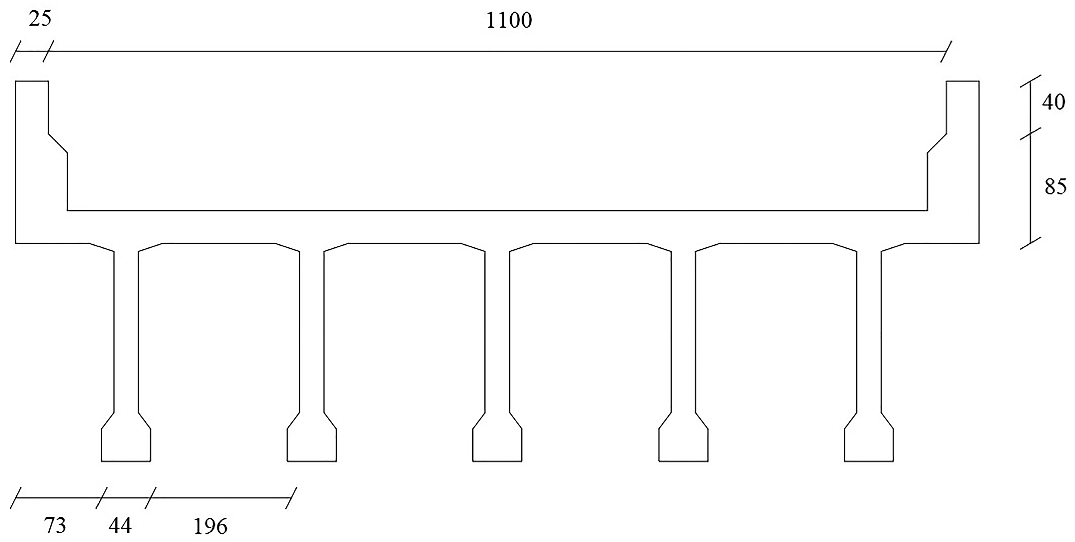
A concrete, simply supported, five T-girder beam bridge is used as the analysis model. Its span is 30 m. The T-girder is 2.50 m high, and the bridge cross-section is shown in Figure 6. The bending moment of inertia of the bridge is $I_z=2.9 {\mathrm{m}}^4$, and the modulus of elasticity for the bridge beam is $E_c=3.25\ast {10}^{10}\mathrm{pa}$. The bridge deck width is 11.50 m, and the left and right anti-collision railings width is 0.50 m.

A classical three-dimensional bridge FEM is developed, and the Euler beam was applied to build the bridge model. The span is divided into 40 finite elements, with an element length of 0.75 m. The main objective is to compute the global dynamic amplification factor of the beam; the detailed structure of the diaphragms and the real connection with the T-girders are not considered during the simulation. Rather, the multi-T-girder section is considered as a whole, and it is assumed that the deck of the bridge is connected rigidly at the top of the T-girders. To consider the transition between the road and bridge, two additional 25 m segments with very large stiffness are added before and after the bridge.

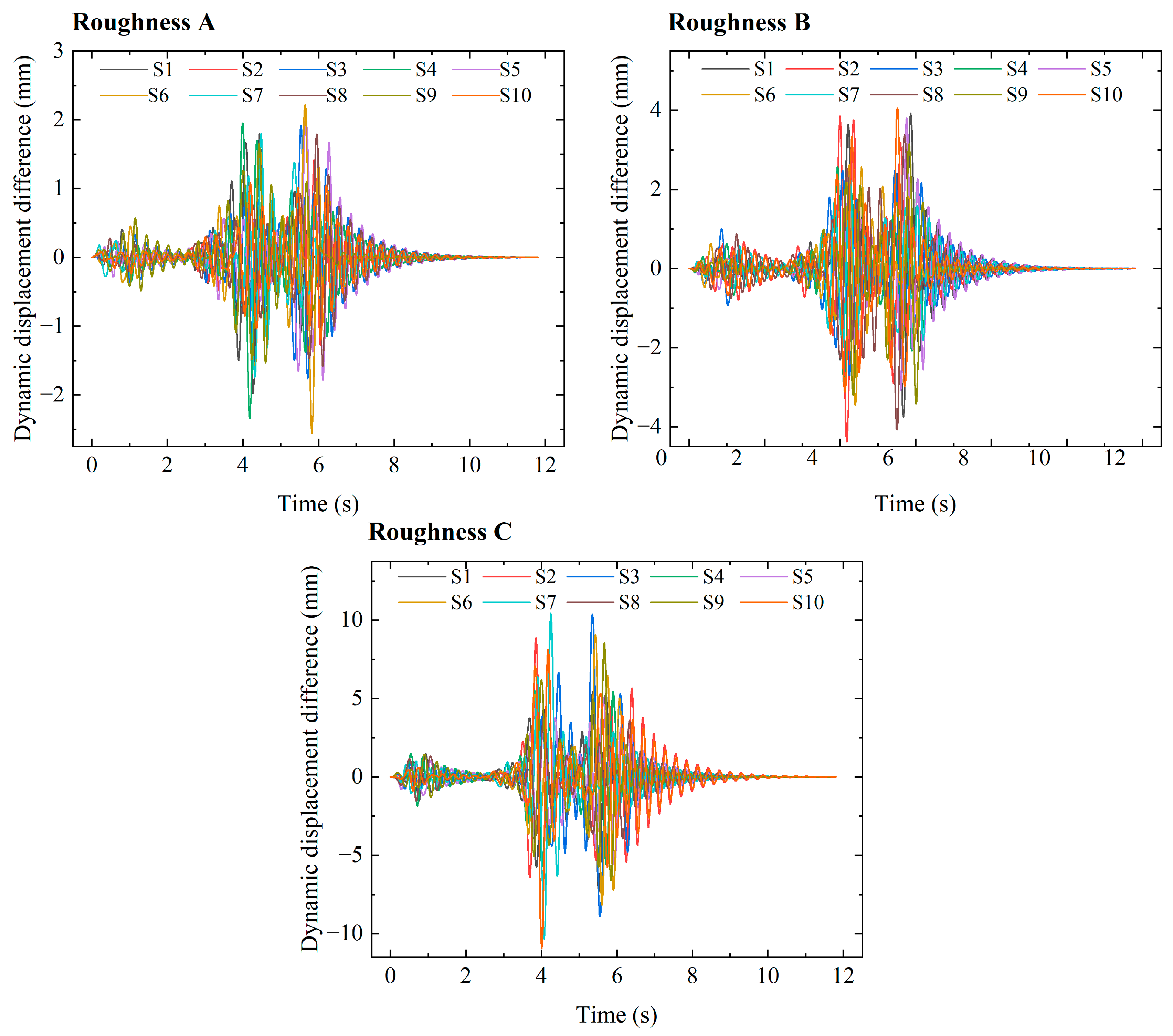
The time history of the $\Delta D$ for the midpoint of the bridge is shown in Figure 7. The first 10 samples of different road roughness levels are considered. For all roughness levels, at the initial stage, the $\Delta D$ is relatively lower, but it shows a significant vibration due to the first impact load from the vehicles during the entry of the bridge. Between 3.5 and 6.5 s, the amplitude of the vibration increases significantly as multiple vehicles pass over the bridge. In this period, the bridge dynamic response becomes higher due to the maximum VBI effects when the vehicle’s tire forces are distributed along the bridge span, and the bridge will be subjected to the combined effect of moving dynamic loads, VBI forces, and road surface-induced excitations. At the final stage, the bridge vibration gradually decreases as the vehicles exit the bridge.

The road irregularity has a significant effect on amplifying the vibration of the bridge’s dynamic responses. For example, road Roughness A generates the smallest $\Delta D$ with a maximum value of 2 mm. The vibration response is relatively stable and symmetrical, which shows that the excitation is primarily dominated by the moving vehicle loads with minimal effect from surface irregularities. However, for Roughness B and C, the excitation becomes larger in amplitude, reaching around 4 mm and 10 mm, respectively. The increased road irregularity contributes to the intense VBI, leading to a higher dynamic response. In general, the $\Delta D$ shows a consistent pattern with the initial excitation stage influenced by the entry impact load, the main vibration stage when multiple vehicles occupied the bridge span, and when the vehicles left the bridge.

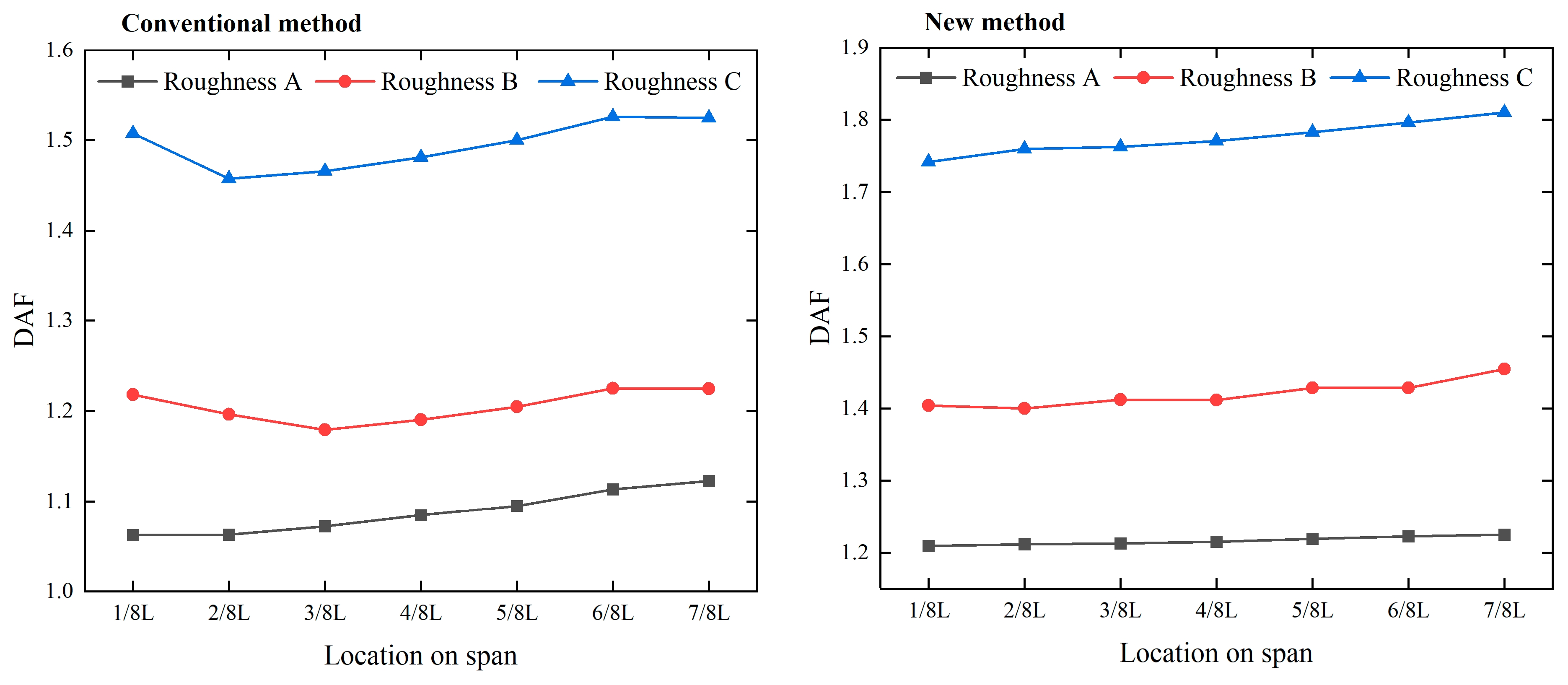
Figure 8 presents the variation in the $DA{F}_N$ for the different locations of the bridge span based on both the conventional (a) and the new method (b). As shown in the figure, it is clearly observed that the DAF values computed from the newly proposed method are consistently larger than the conventional approach for all road roughness levels and span positions. This increase is physically reasonable, as it accounts for the pure dynamic amplification of the bridge response by considering the dynamic displacement difference that compares the bridge dynamic and static responses at exactly the same time steps throughout the entire time history, rather than relying solely on peak dynamic and static responses. Therefore, this newly proposed definition can give realistic and representative DAF values that better reflect the actual dynamic response of the bridge considering the moving vehicular loads.

3. Bayesian POT-GPD Method for Extreme DAF Value Analysis

3.1. The Peaks-over-Threshold–Generalized Pareto Distribution (POT-GPD) Model for DAF

The POT method is an extreme value theory (EVT)-based statistical approach, which is used to model the tail behavior of the exceedances over a specified threshold based on the GPD. It has been widely applied across various areas, including engineering fields, to analyze extreme values. In recent years, the POT framework has gained significant attention for modeling extreme bridge dynamic load effects, as it enables precise quantification of tail behavior by focusing on the most critical exceedances above a threshold, where the extreme dynamic effects are most likely to occur. Considering the exceedances, the GPD can accurately estimate high quantiles and return levels under varying traffic and VBI conditions, even with limited extreme value samples. In this paper, the POT-GPD framework is applied to model the tail distributions of DAF, which are obtained from random traffic–bridge interaction simulations for 200 different cases, where each sample represents one independent realization of stochastic traffic and road roughness. The resulting 200 maximum DAF values are then used as a sample for extreme DAF estimation. The analysis begins with threshold selection to reveal significant exceedances, followed by parameter estimation using both maximum likelihood and Bayesian inference.

In the POT-GPD model, the most important step is selecting the appropriate threshold above which exceedances are modeled by the GPD. To choose a proper threshold, the mean residual life plot (MRLP) is the main tool in identifying the ranges of thresholds according to the GPD assumption.

To choose a threshold, the GPD mean excess function $\mathrm{e}\left(\mathrm{u}\right)$ is defined as

$$e(u)=E\left[X-u|X>u\right]={\displaystyle \frac{\sigma +\xi (u-u_0)}{1-\xi }}, \xi <1$$

(16)

$e(u)$ is the linear function of $u$, and for each candidate threshold $u$, $e(u)$ can be estimated as follows:

$$e(u)={\displaystyle \frac{1}{n_u}}{\displaystyle \sum _{i=1}^{n_u}(X_i}-u) for Xi>u$$

(17)

where $\sigma$ and $\xi$ are the GPD scale and shape parameters at the initial threshold $u_0$, respectively; $u$ is the range of candidate thresholds of the sample data. $X_i$ and $n_u$ are the DAF samples and the number of DAF samples above the threshold, respectively.

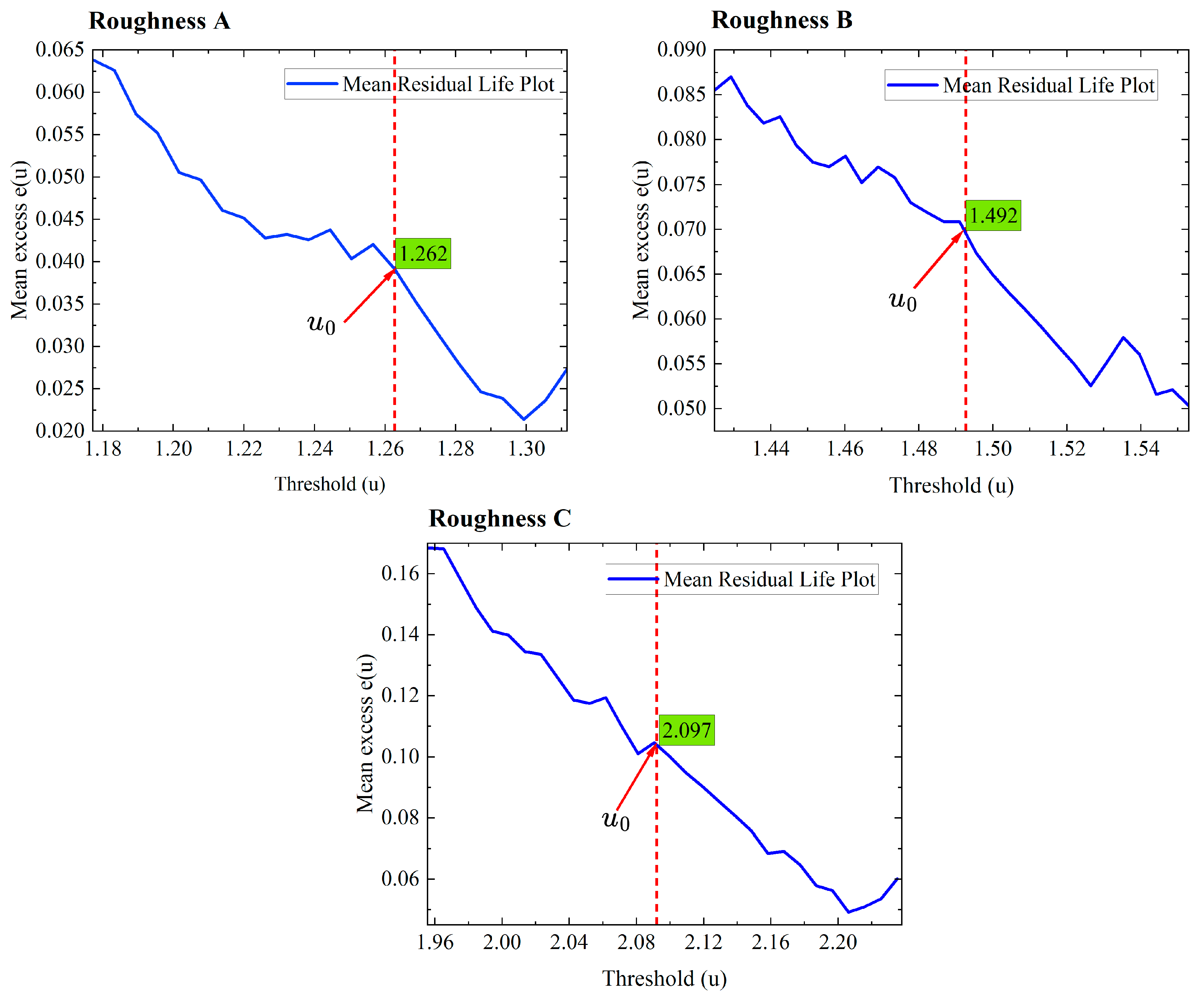
In the threshold choosing process, the first step is determining the range of high candidate thresholds $\mathrm{u}$. For each $\mathrm{u}$, compute the $e(u)$ using Equation (17) and plot MRLP by using the $e(u)$ against $u$ as shown in Figure 9. Next, identify the linear region on the MRLP where $u>u_0$, and the MRLP becomes roughly a straight line. Then, the threshold $u_0$ is selected within this stable, linear region to ensure it is sufficiently high enough to capture the tail behavior of the data while still providing enough exceedances for reliable estimation.

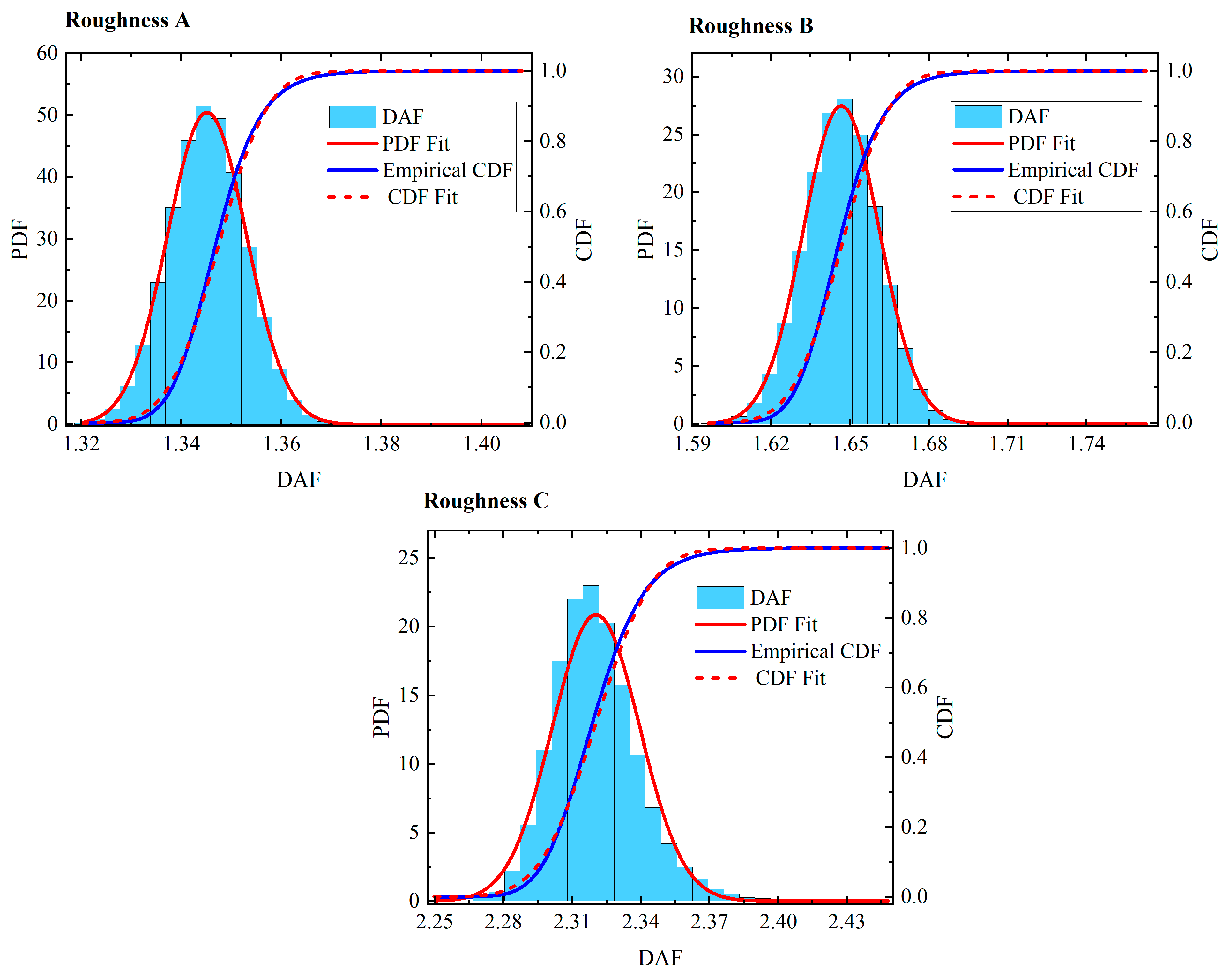
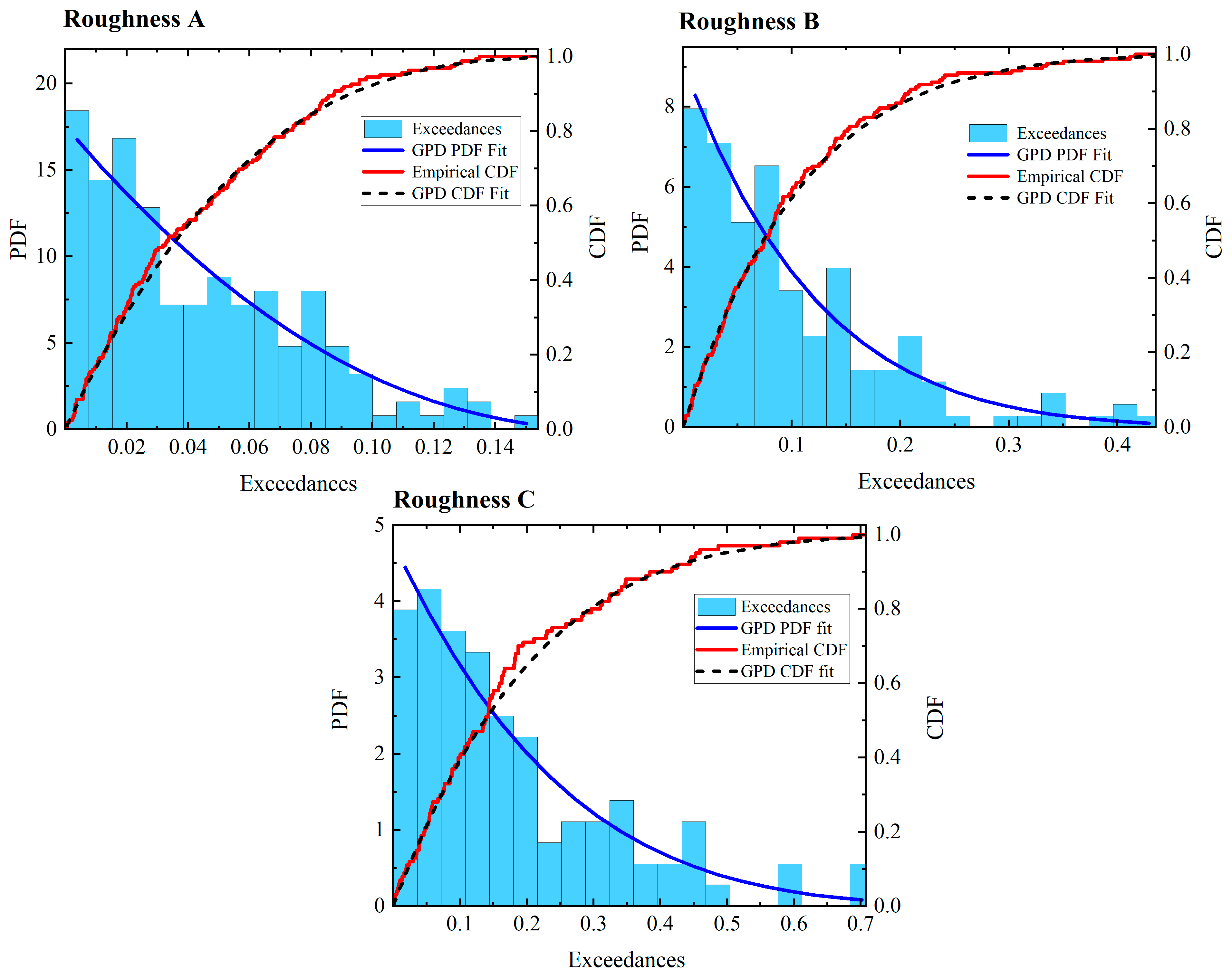
The GPD fit for the exceedances of the DAF data is shown in Figure 10. The results show that for all cases, the theoretical PDF and CDF of the exceedances are well fitted with the empirical GPD fits, indicating that the selected thresholds effectively determine the tail regions of the data, confirming that the GPD model adequately captures the statistical behavior of the exceedances and supporting the reliability of the following return level extreme values estimation. Additionally, the goodness of the GPD model fit is verified using the (K–S) test for all three roughness levels, and the results validated that the fitted GPD distributions are statistically acceptable, reinforcing the adequacy of the model for representing the tail behavior of the DAF exceedances.

After determining the threshold ${\mathrm{u}}_0$, the GPD parameters can be estimated by using the maximum likelihood functions. Let $(x_1,x_2,\dots ,x_m)$ be the DAF samples exceeding the threshold and $y_i=x_i-u_0$ be the exceedances, where $(y_1,y_2,\dots ,y_n)$ follow a GPD with the scale $(\sigma )$ and shape $(\xi )$ parameters, that means $y_i\sim GPD(\sigma ,\xi ), y_i>0$; the likelihood probability density function (PDF) for the GPD model is given as follows:

$$f(y_i|\sigma ,\xi )=\left\{\begin{array}{l}{\displaystyle \frac{1}{\sigma }}{(1+{\displaystyle \frac{\xi y_i}{\sigma }})}^{(-{\displaystyle \frac{1}{\xi }}+1)}, \xi \ne 0 \\ {\displaystyle \frac{1}{\sigma }}\exp (-{\displaystyle \frac{y_i}{\sigma }}), \xi =0 \end{array}\right.$$

(18)

where $y_i$ is the exceedances; $\sigma >0$ is scale parameter; and $y>0$ denotes the exceedance value.

3.2. Bayesian Updates Model for the Extreme DAF Value

In the long-term safety and performance assessment of bridges, particularly with dynamic loading scenarios such as traffic flow–bridge interaction, the accuracy of the predictive models is frequently constrained by the limited sample size. In this case, Bayesian updating provides a probabilistic framework to analyze the extreme values by integrating both the observed data and the prior knowledge, allowing parameter estimates to be refined as more data become available. In the POT-GPD model, the scale and shape parameters’ prior distributions can be obtained from the preliminary maximum likelihood estimates (MLEs). These priors are then updated based on the likelihood of the exceedances to obtain the posterior distributions, which accurately quantify the uncertainty of the parameters even under small sample datasets.

In this paper, Bayesian updating combined with the POT-GPD approach is applied for extreme DAF estimation. According to Bayes’ theorem, for the POT–GPD model, the GPD parameters $\theta =(\sigma ,\xi )$ posterior distribution is expressed as

$$\pi (\theta |y)={\displaystyle \frac{L(y|\theta )\pi (\theta )}{{\displaystyle \int L(y|\theta )\pi (\theta )d\theta }}}$$

(19)

where $\theta =(\sigma ,\xi )$ is the parameters of GPD distribution; $\pi (\theta )$ is the GPD parameters $\theta$ prior distribution; ${\displaystyle \int L(y|\theta )\pi (\theta )d\theta }$ is the marginal probability likelihood of the exceedances; and $L(y|\theta )$ is the likelihood function, which can be derived from the GPD PDF that is expressed as

$$L(\sigma ,\xi |y)={\displaystyle \prod _{i=1}^{n}f(y_i|\theta )}={\displaystyle \prod _{i=1}^{n}f(y_i|\sigma ,\xi )}$$

(20)

where $f(y_i|\theta )$ is the PDF of the GPD model; $y_i$ is the $ith$ exceedance; and $n$ is the number of exceedances.

Since the marginal likelihood in Equation (19) is a normalization constant to ensure the posterior integrates to one, the GPD posterior distribution $\pi (\theta |y)$ can be written as

$$\pi (\theta |y)=L(y|\theta )\pi (\theta )=\pi (\sigma ,\xi |y)=L(y|\theta )\pi (\sigma )\pi (\xi )$$

(21)

Therefore, Bayesian updating requires prior distributions of the GPD parameters $\pi (\sigma )$ and $\pi (\xi )$ to indicate the available knowledge. In this study, the MLE-informed priors’ method is employed, in which the mean and variance of each prior distribution are determined based on the MLE from the DAF datasets. For the priors of GPD parameters, the normal distribution is assumed to generate the prior mean $(\mu )$ and the prior variance $(S^2)$ from the DAF data, with truncation for the scale parameter to ensure positive values, since the negative values are meaningless for scale parameters in probability models. The prior specification is described as

$$\sigma \sim N({\mu }_{\sigma },{S_{\sigma }}^2), \xi \sim N({\mu }_{\xi },{S_{\xi }}^2), \sigma >0$$

(22)

where ${\mu }_{\sigma }$ and ${\mu }_{\xi }$ are the prior mean of the scale and shape parameters, respectively; $({S_{\sigma }}^2)$ and $({S_{\xi }}^2)$ are the prior variance of the scale and shape parameter, respectively.

To estimate the GPD parameter’s posterior distribution, the Markov Chain Monte Carlo (MCMC) method with the Metropolis-within-Gibbs sampler was used to generate the samples from $\pi (\sigma ,\xi |y)$ and iteratively update each parameter. Since the joint posterior distribution $\pi (\sigma ,\xi |y)$ cannot give an explicit solution due to the nonlinearity of the GPD likelihood, the MCMC sampling algorithm provides a complete probabilistic characterization of the parameter to efficiently draw samples from the posterior and estimate the uncertainty of extreme DAF predictions for specified return periods, along with their credible intervals. The detailed MCMC sampling processes are described as follows:

• The initial step is assigning the initial values for the GPD parameters, ${\theta }^{(0)}=({\sigma }^{(0)},{\xi }^{(0)})$. These initials are obtained from the MLE of the GPD parameters. The MLE-informed initialization ensures that the Markov chain begins with a region where the posterior density is high to improve the convergence.
• For each iteration $t (t=1:N)$, where $N$ is the number of iterations, a candidate value for one parameter is generated while the other remains fixed. That means when the scale parameter is updated, the candidate ${\sigma }^{\ast }$ is generated from the proposal distribution, ${\sigma }^{\ast }\sim N({{\mu }_{\sigma }}^{(t-1)},{S_{\sigma }}^2)$ with ${\sigma }^{\ast }>0$ where ${S_{\sigma }}^2$ is the proposal variance, which controls the step size. Similarly, for the shape parameter, the candidate ${\xi }^{\ast }$ is drawn from the proposal distribution ${\xi }^{\ast }\sim N({{\mu }_{\xi }}^{(t-1)},{S_{\xi }}^2)$
• The acceptance probability of a candidate parameter is computed from the probability within the Metropolis-within-Gibbs framework, which alternately updates the GPD parameters.

The acceptance probability for the scale parameter $(\sigma )$ is given by

$${\alpha }_{\sigma }=\min \left\{1,{\displaystyle \frac{\pi ({\sigma }^{\ast },{\xi }^{(t-1)}|y)}{\pi ({\sigma }^{(t-1)},{\xi }^{(t-1)}|y)}}\right\}$$

(23)

Similarly, acceptance probability for the shape parameter ($\mathsf{\xi }$) is given by

$${\alpha }_{\xi }=\min \left\{1,{\displaystyle \frac{\pi ({\sigma }^{(t)},{\xi }^{\ast }|y)}{\pi ({\sigma }^{(t)},{\xi }^{(t-1)}|y)}}\right\}$$

(24)

4.

Iterative updates—steps (2) and (3) are repeated for $N$ iterations. Thus, for each iteration, both the scale and shape parameters are updated sequentially from $({\sigma }^{(t)},{\xi }^{(t)})$ to $({\sigma }^{(t+1)},{\xi }^{(t+1)})$

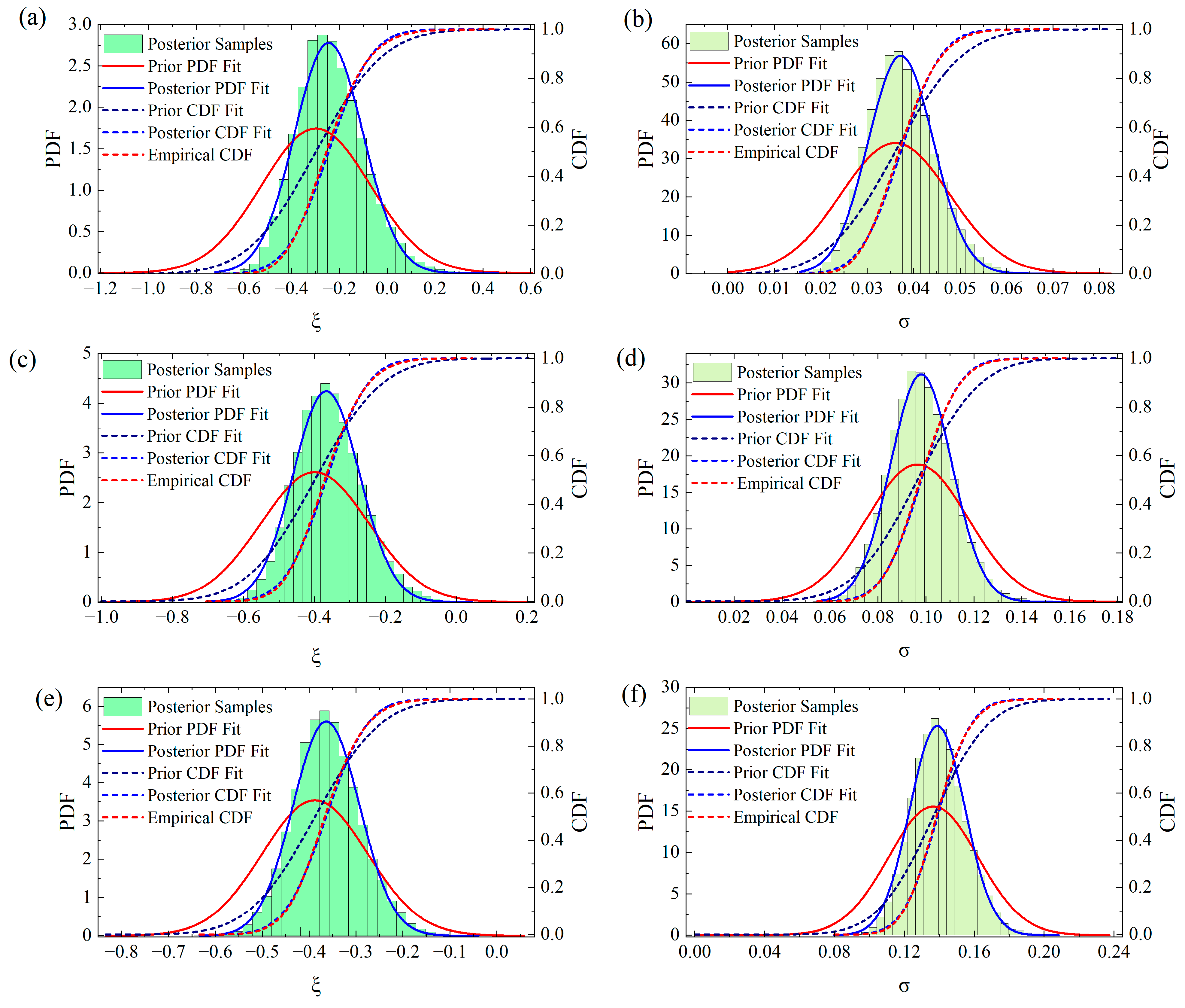
The prior and posterior distributions for the GPD scale and shape parameters are shown in Figure 11. The posterior samples for both parameters show well-converged and symmetric distributions that represent the MCMC sampling effectively capturing the posterior uncertainty. In each case, the prior and posterior PDFs and CDFs are shown to compare the evolution of parameter beliefs after Bayesian updating. The comparison shows that the posterior distributions are more concentrated, indicating reduced uncertainty and improved parameter estimation based on the observed DAF exceedance data. Generally, the results suggest that the MCMC sampling procedure was correctly implemented and provided statistically stable results and physically meaningful posterior estimates for both parameters.

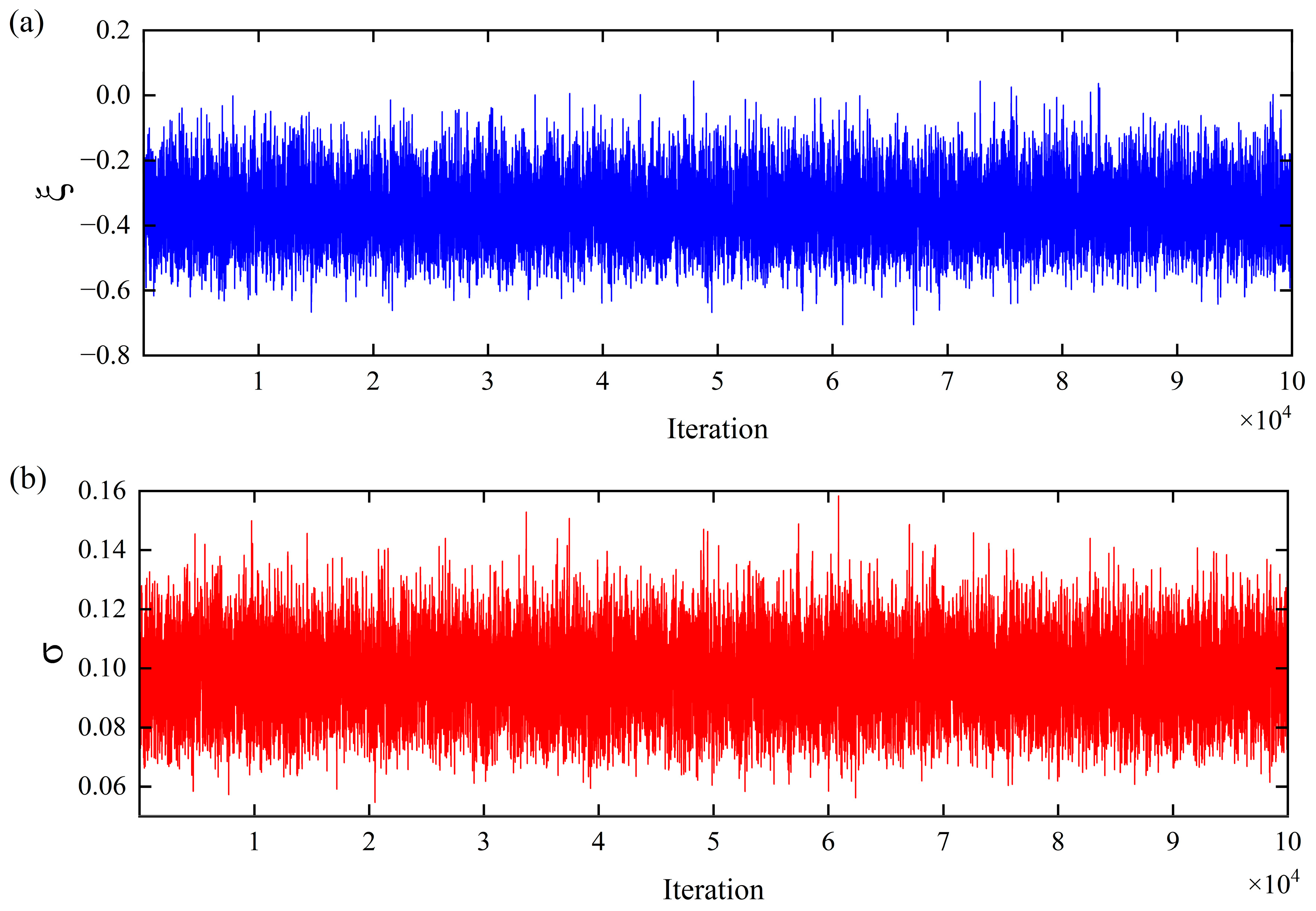
Since the Markov chain is simulated over a large number of iterations, after a certain number of iterations, it converges to stationary distribution. The initial portion of these iterations before MCMC convergence is known as the burn-in period; the sampled values during this period cannot be taken as a sample to model the posterior distribution of the GPD parameters. Therefore, the burn-in period iterations are removed to reduce the influence of starting values, and the remaining values are considered as a stationary chain, which is utilized to analyze the probabilistic behavior of the GPD parameters. To ensure the reliability of the MCMC results, multiple diagnostic tools—such as trace plots, autocorrelation plots, and effective sample size—can be employed to assess chain convergence and stationarity. In this study, trace plots are used as the primary convergence diagnostic because they provide a direct and intuitive visualization of chain mixing and stationarity. Accordingly, the trace plots for both the scale and shape parameters are used to verify chain stationarity, as shown in Figure 12.

4. Prediction of Return Level DAF

The return level DAF prediction refers to the estimation of the extreme DAF values that are expected to occur once within a specified time interval, known as the return period. This concept plays a significant role in structural reliability and bridge design, as it provides the quantitative measure of a bridge’s critical amplification effects arising from extreme dynamic interaction forces between vehicles and bridges due to extreme loading events. Practically, the return period DAF offers a probabilistic measure of the bridge’s extreme dynamic response over time, serving as a key identification for the evaluation of long-term bridge safety and performance.

According to the POT-GPD approach, the return level $DA{F}_T$ for a specific return period $T$ can be derived from the quantile function of the GPD parameters. For $T$ observation period, the DAF of the return level can be given by

$$DA{F}_T=\left\{\begin{array}{l}{u}_0+{\displaystyle \frac{\sigma }{\xi }}{({\lambda }_{u}T)}^{\xi }-1, \xi \ne 0\\ u_0+\sigma \ln ({\lambda }_{u}T), \xi =0\end{array}\right.$$

(25)

where $DA{F}_T$ is the return level DAF; $u_0$ is the threshold; ${\lambda }_u$ represents the exceedance rate, and it can be defined as $({\lambda }_u={\displaystyle \frac{n_u}{N}})$, where $n_u$ and $N$ is the number of exceedances above threshold and the total number of sample data, respectively.

4.1. Effect of the Road Roughness, and Return Periods on Extreme DAF Values

The estimated DAFs for a 50-year return period are shown in Figure 13. For all roughness levels, the fitted PDFs align closely with the observed histograms, demonstrating that the selected statistical model accurately characterizes the distribution of DAFs. The empirical and fitted CDFs also show good agreement, confirming that the model reliably captures the upper-tail behavior that governs extreme value estimation. A consistent trend is observed as road roughness worsens: the distribution of DAF shifts to higher values and becomes more dispersed. For Roughness A, the mean DAF is approximately 1.35, indicating relatively mild amplification under smoother surface conditions. For Roughness B, the mean increases to about 1.65, reflecting a noticeable rise in dynamic response. Under Roughness C, the mean DAF further increases to roughly 2.32, showing that poor surface quality significantly amplifies bridge dynamic effects.

The results clearly demonstrate that rougher road profiles lead not only to larger expected DAF values with return periods but also to greater variability in the extreme response. These findings underscore the importance of incorporating road roughness conditions when evaluating long-term dynamic performance and safety margins of bridges.

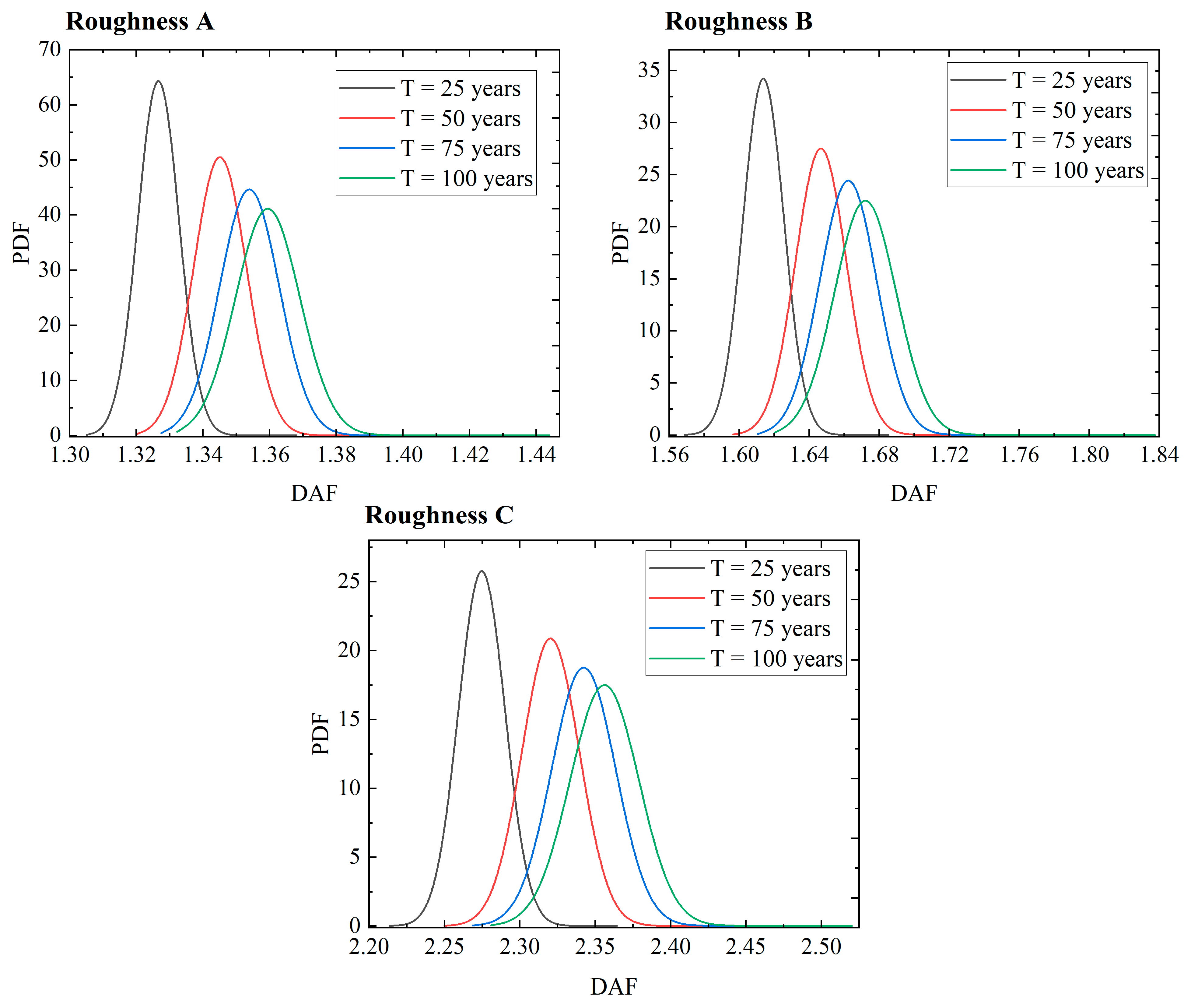
To further investigate the effect of the return periods, the estimated DAF probability distributions for different return periods are shown in Figure 14. It is clearly shown that for all roughness levels, the probability density curves gradually decrease with increasing return periods. This reduction in peak PDF values is related to that, as the return period increases, the predicted DAFs correspond to rarer and more extreme dynamic responses, which are statistically less probable to occur within shorter time intervals. As a result, the distribution becomes wider and flatter, reflecting higher uncertainty and variability in DAF as the return period extends. At the same time, the mean DAF of each distribution gradually shifts toward higher DAF values with increasing return periods, indicating that the expected extreme DAF intensifies over longer return periods.

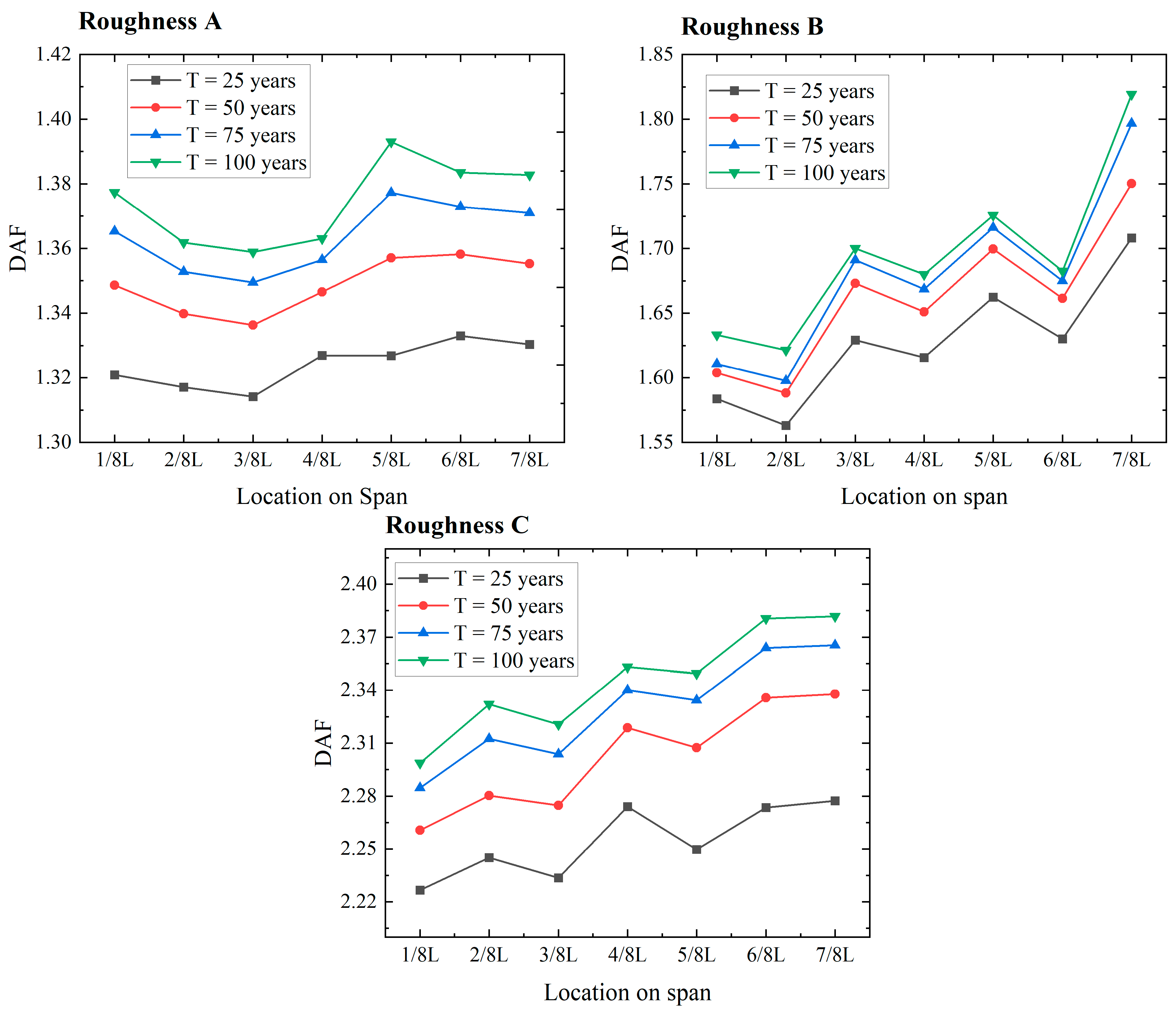
Figure 15 presents the spatial variation in return level extreme DAF values along the bridge span. For all cases, the extreme DAF consistently increases with longer return periods, reflecting the higher probability of experiencing more severe dynamic amplification over extended time horizons. It should be noted that DAF is dependent on the maximum dynamic and static response at a given location. While the maximum static response at different positions along the span is deterministic and governed primarily by structural properties and load positions, the magnitude and, more importantly, the occurrence time of the maximum dynamic response are strongly influenced by the spatial distribution of road roughness. For roughness levels B and C, the random distribution of roughness heights excites the vehicle–bridge system differently as vehicles traverse the span, leading to localized amplification of dynamic responses at certain positions (e.g., 5/8 L and 7/8 L). As a result, the peak dynamic response does not necessarily coincide spatially with the peak static response, producing nonuniform and location-dependent DAF values along the span. The influence of road roughness is also evident: smoother surfaces produce lower and more uniform DAF distributions, whereas moderate and especially severe roughness led to substantially higher DAFs and more pronounced spatial fluctuations along the span. Across all roughness levels, the 1/8 L to 7/8 L positions show similar trends, with critical locations generally aligning with mid- to right-end span regions where dynamic response is typically amplified. Therefore, the PDF curves and the estimated extreme DAFs confirm that both increasing return period and road roughness increase the expected DAF magnitude while simultaneously reducing the probability density, capturing the dual effect of extremity and uncertainty in bridge dynamic response prediction.

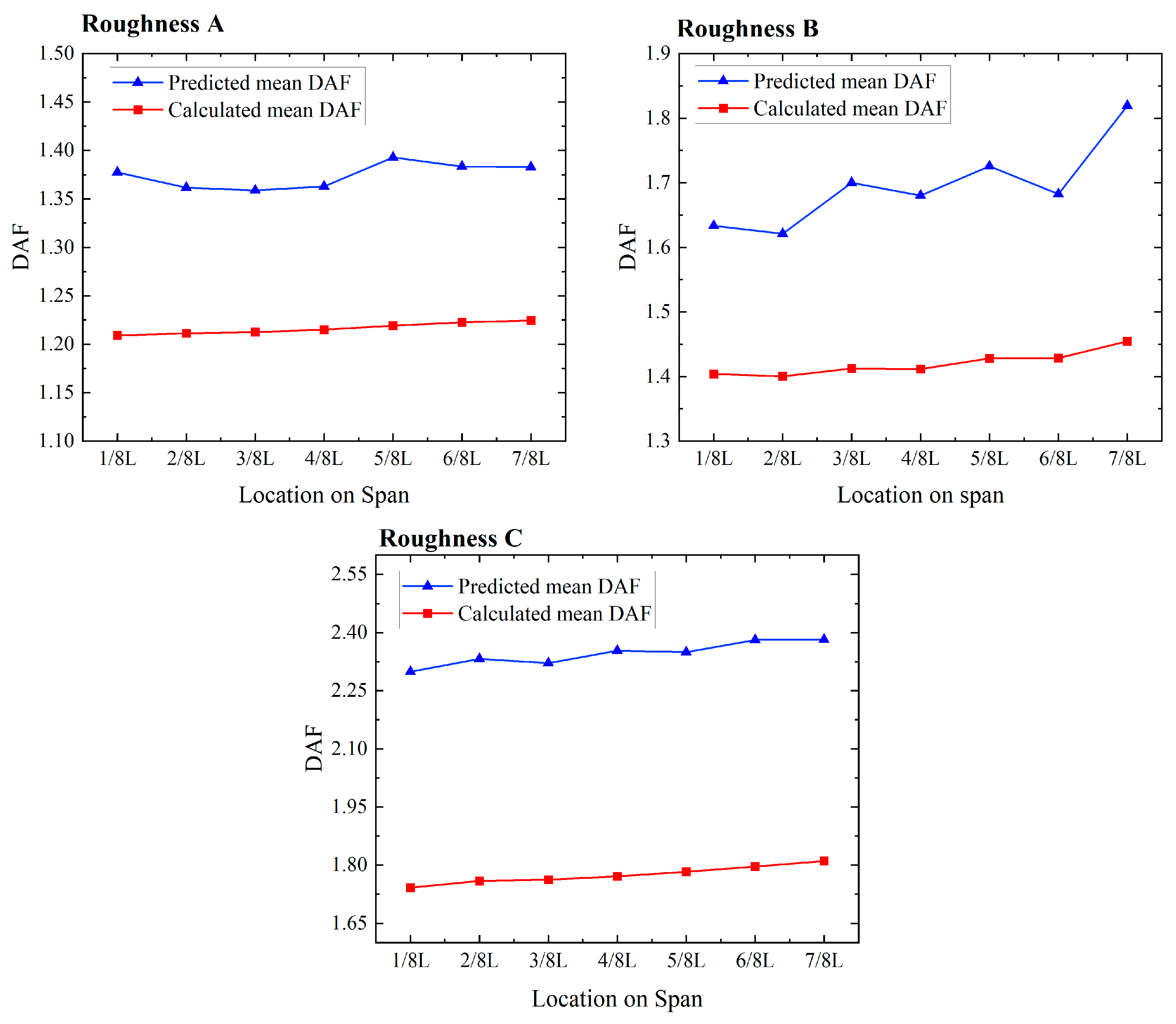
The predicted mean extreme DAFs for a 100-year return period are compared with the actual calculated mean DAFs obtained directly from the bridge response in Figure 16. As shown in the figure, the predicted mean extreme DAFs are consistently higher than the originally calculated mean values. This indicates that, over longer time, rare but severe dynamic events lead to a systematic upward shift in the expected DAF, reflecting the cumulative effect of extreme traffic–bridge interaction conditions. Although the originally calculated mean DAFs capture the average dynamic response under the traffic scenarios, the predicted extreme DAFs provide a more realistic basis for evaluating long-term bridge safety and reliability.

4.2. Comparison Between GPD- and GEV-Based Extreme DAF Values

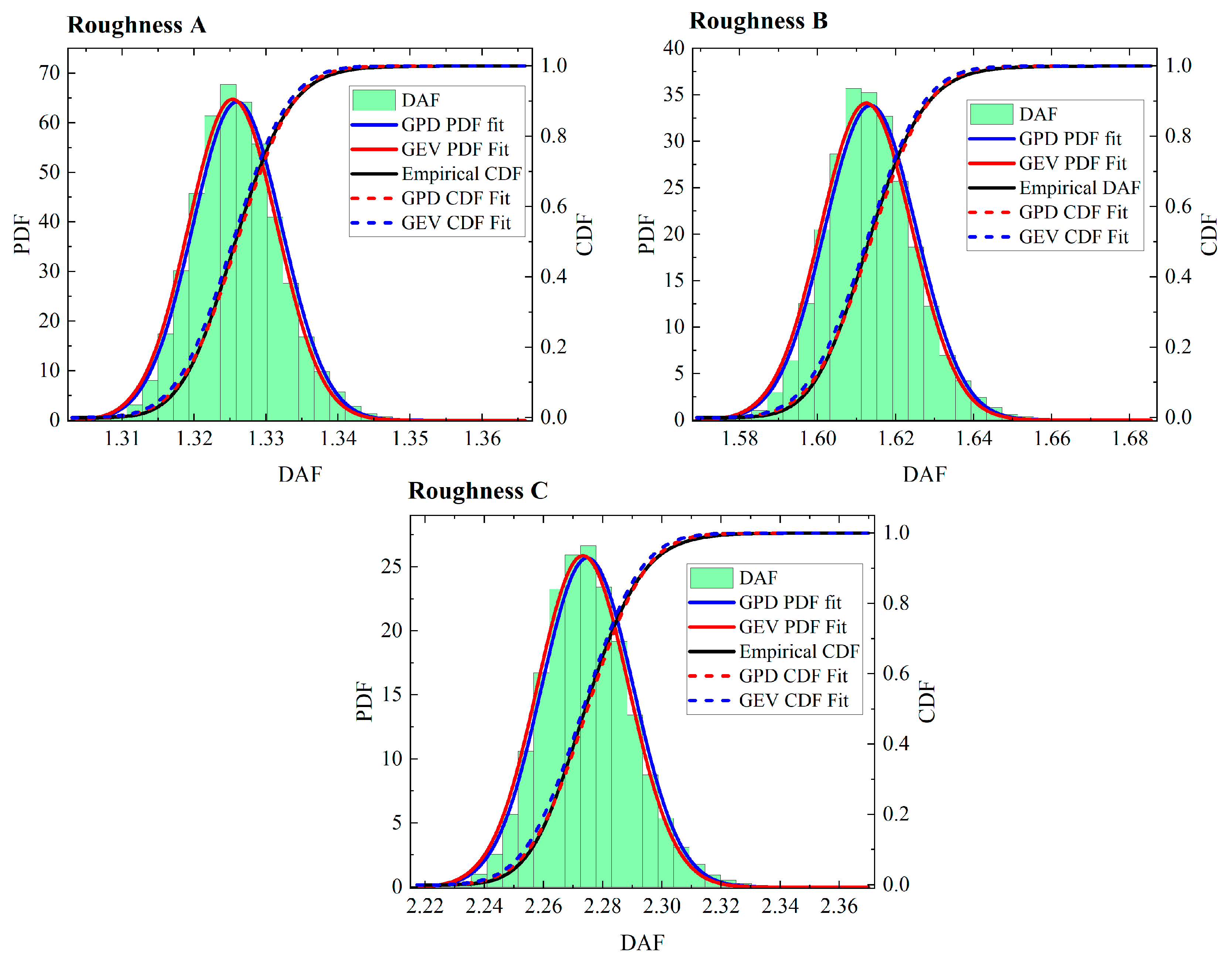
The predicted DAF distributions obtained from the GPD- and GEV-based models are presented in Figure 17. Although both models are grounded in EVT, they differ in the extraction and representation of the extreme values. As mentioned in Section 3, the GPD model is based on the exceedances over a selected threshold, while the GEV model is based on the block maxima (daily, monthly, or annual maxima). However, in this study, the block maxima are not directly applied for the GEV model since the available DAF samples are limited and not well suited for partitioning into different independent blocks. Instead, the GEV parameters can be derived from the GPD parameters theoretically through the Poisson process formulation that enables an equivalent comparison between the two methods. In this approach, threshold exceedance events are independent and follow a Poisson process, as the DAFs are derived from independent VBI simulations with random traffic flow and road roughness profiles, which reasonably supports the independence assumption. Moreover, exceedances are defined over a sufficiently high threshold, and their occurrence rate remains approximately stable, making the Poisson process reasonable for the DAF data considered. According to the Poisson process framework, the occurrence of over a sufficiently high threshold can be modeled as a non-homogeneous Poisson process, where the rate of exceedance and the magnitudes of exceedances jointly describe the tail characteristics of the distribution. This formulation provides a consistent probabilistic foundation that links the GPD and GEV distributions. Under this approach, the shape parameters for both models are equivalent $(\xi ={\xi }_{GPD}={\xi }_{GEV})$, while the GEV scale $({\sigma }_{GEV})$ and location $({\mu }_{GEV})$ parameters can be derived from the corresponding GPD scale parameter $({\sigma }_{GPD})$, threshold level $(u_0)$, and the exceedance rate $({\lambda }_u)$ as follows:

$${\sigma }_{GEV}={\sigma }_{GPD}{({\lambda }_{u}T)}^{\xi }, and {\mu }_{GEV}=u_0-{\displaystyle \frac{{\sigma }_{GPD}}{\xi }}[1-{({\lambda }_{u}T)}^{\xi }$$

(26)

The corresponding return level DAF $(DA{F}_T)$ associated with a given return period $T$ can be expressed directly from the GEV distribution as

$$DA{F}_T={\mu }_{GEV}+{\displaystyle \frac{{\sigma }_{GEV}}{\xi }}[{(-\ln (1-{\displaystyle \frac{1}{T}}))}^{-\xi }-1]$$

(27)

This process offers a direct comparison between the location, scale, and shape characteristics of the predicted extreme DAF distributions under a well-structured probabilistic framework. Interpreting the results from both models allows for investigating whether the DAF extremes calculated from threshold exceedances (GPD) align with those obtained from the equivalent GEV representation, thus validating the statistical coherence of the extreme value modeling approach.

As shown in Figure 17, both the PDF and CDF of the GPD and GEV fitting curves show strong agreement with the predicted DAF data, demonstrating a close consistency between the two models. The probability density becomes lower and more spread out with increasing road roughness, indicating that the extreme DAF events become less frequent but more severe. It also confirms the statistical nature of extreme events: that higher return levels of DAFs are associated with lower occurrence probabilities, resulting in flatter and wider distributions. Overall, the strong agreement between GPD and GEV fits, even under varying road irregularity conditions, validates the robustness of the Poisson-based derivation and confirms that both models effectively capture the probabilistic structure of long-term DAF extremes. The numerical results are described in

Table 1. The 95% confidence interval return level DAFs at the midspan of the bridge.

Roughness A
Return Period (years)	GPD model			GEV model
	Mean	Min	Max	Mean	Min	Max
25	1.327	1.315	1.339	1.326	1.314	1.338
50	1.347	1.331	1.362	1.347	1.331	1.362
75	1.357	1.339	1.374	1.357	1.339	1.374
100	1.363	1.344	1.382	1.362	1.342	1.382
Actual calculated DAFs (200 samples)	Mean		Min		Max
	1.214		1.110		1.336
Roughness B
Return Period (years)	GPD model			GEV model
	Mean	Min	Max	Mean	Min	Max
25	1.616	1.593	1.639	1.615	1.592	1.637
50	1.651	1.623	1.679	1.651	1.622	1.679
75	1.669	1.637	1.700	1.664	1.637	1.691
100	1.680	1.646	1.714	1.680	1.646	1.714
Actual calculated DAFs (200 samples)	Mean		Min		Max
	1.412		1.173		1.550
Roughness C
Return Period (years)	GPD model			GEV model
	Mean	Min	Max	Mean	Min	Max
25	2.277	2.247	2.306	2.275	2.246	2.305
50	2.325	2.288	2.362	2.325	2.288	2.361
75	2.349	2.308	2.390	2.349	2.308	2.389
100	2.365	2.321	2.408	2.364	2.320	2.408
Actual calculated DAFs (200 samples)	Mean		Min		Max
	1.771		1.382		2.283

.

As shown in Table 1, the DAFs predicted by both the GPD and GEV models are substantially higher than the actual calculated DAFs obtained from the finite sample of 200 simulations. While the sample-based DAFs reflect typical dynamic responses observed within the limited observation period, the extreme value models explicitly extrapolate the upper tail of the DAF distribution to longer return periods, thereby accounting for rare but potentially critical VBI events that are unlikely to appear in the available samples. The close agreement between GPD- and GEV-based estimates further confirms the accuracy of the extreme value predictions, while the higher return level DAFs emphasize that relying only on directly calculated sample values may significantly underestimate the long-term extreme dynamic amplification.

For both GPD and GEV models, the estimated shape parameter $(\xi )$ is negative (

Table 2. The estimated GPD and GEV parameters and their corresponding upper bound values.

Road Roughness	GPD Model			GEV Model
	Parameters	Estimated Mean Value	Upper Bound	Parameters	Estimated Mean Value	Upper Bound
A	$u_0$	1.26694	$DA{F}_{up}$ = 1.412	$\mu$	1.14493	$DA{F}_{up}$ = 1.417
	$\sigma$	0.05085		$\sigma$	0.09602
	$\xi$	−0.35308		$\xi$	−0.35308
B	$u_0$	1.49279	$DA{F}_{up}$ = 1.762	$\mu$	1.28259	$DA{F}_{up}$ = 1.771
	$\sigma$	0.09786		$\sigma$	0.17779
	$\xi$	−0.36401		$\xi$	−0.36401
C	$u_0$	2.09748	$DA{F}_{up}$ = 2.481	$\mu$	1.81922	$DA{F}_{up}$ = 2.488
	$\sigma$	0.13888		$\sigma$	0.24231
	$\xi$	−0.36226		$\xi$	−0.36226

), indicating that the extreme value distribution demonstrates a finite upper bound. This condition suggests that the modeled variable has a natural statistical limit beyond which exceedances are theoretically improbable.

The CDF of the GEV distribution can be expressed as

$$G(z)=\exp \left\{-\left[1+\xi ({\displaystyle \frac{z-\mu }{\sigma }}){]}^{-{\displaystyle \frac{1}{\xi }}}\right]\right\}, and 1+\xi \left({\displaystyle \frac{z-\mu }{\sigma }}\right) >0$$

(28)

where $\sigma$, $\xi$, and $\mu$ represent the scale, shape, and location parameters, respectively. When $\xi <0$, the support of the distribution is bounded above by the point where $1+\xi ({\displaystyle \frac{z-\mu }{\sigma }})>0$, yielding the theoretical upper bound DAF as

$$DA{F}_{up}=\mu -{\displaystyle \frac{\sigma }{\xi }}, for (\xi <0)$$

(29)

Similarly, for the GPD model, which describes exceedances $y=X-u_0$ over a threshold $u_0$, the CDF is given by

$$G(y)=1-{\left(1+\xi {\displaystyle \frac{y}{{\sigma }_{u_0}}}\right)}^{-{\displaystyle \frac{1}{\xi }}}, and 1+\xi {\displaystyle \frac{y}{{\sigma }_{u_0}}}>0$$

(30)

where ${\sigma }_{u_0}$ is the GPD scale parameter at the threshold $u_0$. When $\xi <0$, the exceedances are limited to $y<-{\displaystyle \frac{{\sigma }_{u_0}}{\xi }}$, and the corresponding upper bound DAF for the original variable is

$$DA{F}_{up}=u_0-{\displaystyle \frac{{\sigma }_{u_0}}{\xi }}, for (\xi <0)$$

(31)

A negative shape parameter is obtained for all roughness levels, which means the extreme DAF value distribution follows the Weibull (Type III) extreme value family, confirming the distribution has a finite right endpoint. This implies that the extreme DAF values are statistically bounded, and no values larger than $DA{F}_{up}$ are expected to happen under the modeled VBI system and road roughness conditions. Physically, this indicates that even under the most adverse dynamic loading cases, the DAF will not exceed $DA{F}_{up}$ but will approach a limiting value determined by the dynamic properties of the VBI system. Therefore, these upper bound values can serve as an important indicator of the maximum expected amplification response of the bridge, a probabilistic limit useful for reliability assessment and safety design. However, it should be explained as a model-based upper limit, subject to uncertainty mainly from the threshold selection, sample size, and parameter estimation.

4.3. Comparison with the Design Codes

According to different countries’ design codes, there is a significant variation between DAF values. For instance, the AASHTO design code [46] specifies constant DAF values of 1.15 and 1.33 for fatigue limit states and all other limit states, respectively. Similarly, the Canadian design code [47] adopts fixed DAF values of 1.4, 1.3, and 1.25 for single, two, and multi-axle vehicles classifications, respectively. The Chinese design code [48] defines three DAF values depending on the first-order bending frequency, with the third case (1.36) taken in this study. In contrast, the New Zealand [49] and Japanese design codes [50] express DAF based on the span length, given by $1+{\displaystyle \frac{15}{(L+38)}}$ and $1+{\displaystyle \frac{7}{(L+20)}}$, respectively. The British Standard BS 5400 [51] assumes a 25% dynamic load allowance for both normal and abnormal traffic conditions, corresponding to a DAF of 1.25. A summary of DAF values from various international design codes is presented in

Table 3. DAF values of different countries design code at 30 m simply supported bridge.

AASHTO	Canadian	Chinese	New Zealand	Japanese	British
1.33	1.3	1.36	1.22	1.14	1.25

. Overall, considerable differences exist between the codes’ values, as the Chinese AASHTO and Canadian codes tend to adopt more conservative DAF values.

As shown in

Table 4. The estimated mean DAFs for a 50-year return period.

Location on Span	Roughness A	Roughness B	Roughness C
1/8 L	1.348	1.603	2.260
2/8 L	1.339	1.588	2.280
3/8 L	1.336	1.672	2.274
4/8 L	1.346	1.651	2.318
5/8 L	1.357	1.699	2.307
6/8 L	1.358	1.661	2.335
7/8 L	1.355	1.750	2.337

, the estimated mean DAFs at a 50-year return period for all bridge locations exceed the values prescribed by different international design codes. For Roughness A, the mean DAFs range from 1.336 to 1.358, which is comparable to the Chinese, AASHTO, and Canadian codes, indicating that these standards reasonably represent long-term dynamic effects on well-maintained surfaces. However, for Roughness B and Roughness C road surface conditions, the estimated DAFs increase significantly, reaching 1.60–1.88 and 2.26–2.34, respectively, values that far exceed all code-based limits. These higher DAFs reflect an increased dynamic demand on the bridge structure under realistic VBI and road roughness conditions. Furthermore, the stochastic traffic–bridge interaction (VBI) model used in this study explicitly simulates random traffic flow, vehicle types, axle loads, speeds, lane distributions, and road roughness. This allows dynamic load effects to arise naturally from vehicle–bridge interaction. In contrast, most design codes adopt simplified deterministic or semi-deterministic load models, such as equivalent uniformly distributed loads or standard design vehicles, combined with a fixed dynamic amplification factor (DAF) to conservatively represent average dynamic effects. Code-specified DAF values are typically calibrated using empirical observations, simplified dynamic analyses, and safety margins. In this way, uncertainties related to traffic variability, road roughness, and long-term extreme effects are only implicitly considered. However, this implicit treatment does not explicitly distinguish the effects of traffic randomness and site-specific roughness. These effects are directly captured in this study through stochastic simulation and extreme value analysis. The results demonstrate that DAF is not a single fixed value. Instead, it varies with traffic characteristics, road roughness, and the target return period. This highlights the potential of stochastic VBI-based extreme DAF estimates to support performance-based or reliability-informed design. Consequently, code-specified DAF values could be refined for specific bridge types, traffic conditions, and serviceability or safety limit states, rather than relying on uniform conservative values. Therefore, the findings indicate that existing design provisions, which generally assume ideal or moderately smooth pavement conditions, may underestimate dynamic effects for deteriorated road surfaces and long return periods. This underscores the need to incorporate road roughness and long-term stochastic effects into bridge design and assessment practices.

5. Conclusions

Although many methods have been developed to estimate general extreme dynamic load effects on bridges, research specifically focused on extreme DAFs remains very limited. To address these gaps, this paper develops an integrated framework that combines realistic random traffic–bridge dynamic simulation, a refined DAF definition, and a POT-GPD combined with Bayesian extreme value analysis to provide more physically meaningful predictions of extreme DAFs. Finally, the following conclusions are drawn:

• The POT–GPD framework, integrated with Bayesian updating, proved highly effective in modeling the statistical distribution and tail behavior of extreme DAF values. By incorporating Bayesian inference with MCMC sampling, the approach rigorously quantifies uncertainty in the GPD parameters, enabling reliable extrapolation of return level DAFs even with limited samples and providing a better probabilistic basis for long-term bridge dynamic performance assessment.
• The predicted results demonstrate that extreme DAFs are strongly influenced by both road roughness and return period, with deteriorating surface conditions leading to markedly higher magnitudes and variability of DAFs and longer return periods corresponding to more severe expected extremes. Comparison between the POT–GPD and equivalent GEV models shows strong consistency, with negative shape parameters (ξ) across all roughness levels, indicating a Weibull (Type III) distribution and implying a finite probabilistic upper bound for extreme DAFs under the modeled VBI conditions.
• Comparison with international design codes indicates that code-based DAF values may be adequate for well-maintained road surfaces but may become increasingly non-conservative as pavement conditions deteriorate. From an engineering perspective, the proposed framework provides a practical and powerful tool for predicting extreme DAFs associated with specified return periods, which is critically important for long-term bridge safety assessment. By supporting reliability-based design and evaluation under stochastic traffic loading and varying road roughness conditions, the proposed approach enables more informed, risk-aware decision-making for bridge design and maintenance.

Future Research Direction

While this study provides valuable insights into the prediction of the dynamic amplification factor (DAF) of bridges using vehicle–bridge interaction (VBI) analysis, some limitations remain. The investigation is primarily focused on short- and medium-span simply supported bridges and does not include extensive field validation or reliability-based design considerations. Future research should focus on validating the proposed models with comprehensive field measurements, integrating reliability-based design frameworks to account for uncertainties in bridge and traffic parameters, and extending the analysis to long-span bridges to generalize the approach to more complex structural systems.

References

1. Obrien, E.J.; Cantero, D.; Enright, B.; González, A. Characteristic Dynamic Increment for extreme traffic loading events on short and medium span highway bridges. Eng. Struct. 2010, 32, 3827–3835. [Google Scholar] [CrossRef] [Scilit]
2. Caprani, C.C.; González, A.; Rattigan, P.H.; Obrien, E.J. Assessment dynamic ratio for traffic loading on highway bridges. Struct. Infrastruct. Eng. 2012, 8, 295–304. [Google Scholar] [CrossRef] [Scilit]
3. Cai, C.S.; Zhang, W.; Deng, L.; Xia, M. Performance Evaluation of Existing Bridges under Vehicle Dynamic Effects. Adv. Mater. Res. 2013, 639–640, 42–53. [Google Scholar] [CrossRef] [Scilit]
4. Kafshgarkolaei, H.J.; Lotfollahi-Yaghin, M.A.; Mojtahedi, A. A modified orthonormal polynomial series expansion tailored to thin beams undergoing slamming loads. Ocean Eng. 2019, 182, 38–47. [Google Scholar] [CrossRef] [Scilit]
5. Bagheri, M.; Malidarreh, N.R.; Ghaseminejad, V.; Asgari, A. Seismic resilience assessment of RC superstructures on long–short combined piled raft foundations: 3D SSI modeling with pounding effects. Structures 2025, 81, 110176. [Google Scholar] [CrossRef] [Scilit]
6. Zhou, X.-Y.; Schmidt, F.; Toutlemonde, F.; Jacob, B. A mixture peaks over threshold approach for predicting extreme bridge traffic load effects. Probabilistic Eng. Mech. 2016, 43, 121–131. [Google Scholar] [CrossRef] [Scilit]
7. Rostami, M.; Yahya, M.B.A.; Yahya, M.H.; Ibrahim, N.A. Slice sampler algorithm for generalized Pareto distribution. Hacet. J. Math. Stat. 2017, 47, 1–32. [Google Scholar] [CrossRef] [Scilit]
8. Liu, Y.; Li, D.; Li, Y.; Zhang, Z. Estimation of Extreme Value Vehicle Load Based on the Extended Burr XII Distribution. KSCE J. Civ. Eng. 2017, 22, 3401–3408. [Google Scholar] [CrossRef] [Scilit]
9. Xu, L.; Tan, S.; Wang, R.; Kang, M.; Zhou, J. Effective temperature determination for long-span steel truss arches: Experimental and numerical investigations. Structures 2025, 81, 110282. [Google Scholar] [CrossRef] [Scilit]
10. Deng, Y.; Li, A.; Chen, S.; Feng, D. Serviceability assessment for long-span suspension bridge based on deflection measurements. Struct. Control. Heal. Monit. 2018, 25, e2254. [Google Scholar] [CrossRef] [Scilit]
11. Zhou, J.; Hu, C.; Chen, Z.; Wang, X.; Wang, T. Extreme value modeling of coincident lane load effects for multi-lane factors of bridges using peaks-over-threshold method. Adv. Struct. Eng. 2020, 24, 539–555. [Google Scholar] [CrossRef] [Scilit]
12. Wang, Q.-A.; Chen, J.; Ni, Y.; Xiao, Y.; Liu, N.; Liu, S.; Feng, W. Application of Bayesian networks in reliability assessment: A systematic literature review. Structures 2024, 71, 108098. [Google Scholar] [CrossRef] [Scilit]
13. Jacinto, L.; Neves, L.C.; Santos, L.O. Bayesian assessment of an existing bridge: A case study. Struct. Infrastruct. Eng. 2015, 12, 61–77. [Google Scholar] [CrossRef] [Scilit]
14. Yu, Y.; Cai, C.S. Prediction of Extreme Traffic Load Effects of Bridges Using Bayesian Method and Application to Bridge Condition Assessment. J. Bridg. Eng. 2019, 24, 1357. [Google Scholar] [CrossRef] [Scilit]
15. Ni, Y.; Wang, Y.; Zhang, C. A Bayesian approach for condition assessment and damage alarm of bridge expansion joints using long-term structural health monitoring data. Eng. Struct. 2020, 212, 110520. [Google Scholar] [CrossRef] [Scilit]
16. Rizqiansyah, A.; Caprani, C.C. Hierarchical Bayesian modeling of highway bridge network extreme traffic loading. Struct. Saf. 2024, 111, 102503. [Google Scholar] [CrossRef] [Scilit]
17. Yan, X.; Jia, S.; Jia, S.; Gao, J.; Peng, J. Bayesian Inference and Condition Assessment Based on the Deflection of Aging Reinforced Concrete Hollow Slab Bridges. Buildings 2024, 14, 2920. [Google Scholar] [CrossRef] [Scilit]
18. Wang, X.; Ruan, X.; Casas, J.R.; Zhang, M. Probabilistic model of traffic scenarios for extreme load effects in long-span bridges. Struct. Saf. 2023, 106, 102382. [Google Scholar] [CrossRef] [Scilit]
19. Li, H.; Wang, T.; Wu, G. A Bayesian deep learning approach for random vibration analysis of bridges subjected to vehicle dynamic interaction. Mech. Syst. Signal Process. 2022, 170, 108799. [Google Scholar] [CrossRef] [Scilit]
20. O’bRien, E.J.; Wilson, S.; Keenahan, J.; Ren, Y. A Bayesian Approach to the Estimation of Road Profile and Bridge Damage from a Fleet Passing Vehicle Measurements. Int. J. Struct. Stab. Dyn. 2023, 24, 24. [Google Scholar] [CrossRef] [Scilit]
21. Zhang, P.J.; Wang, C.S. Analysis on temperature action of high-speed railway steel bridges and prediction for temperature based on small-scale data set. Structures 2025, 80, 109708. [Google Scholar] [CrossRef] [Scilit]
22. Luo, L.; Li, Y.; Dai, H.; Sun, H.; Jia, M.; Yuan, H.; Cheng, X. Seismic performance prediction and interpretation of RC bridges under vehicle-bridge interaction: From VBI system simulation to ensemble learning surrogate models. Eng. Struct. 2025, 341, 120816. [Google Scholar] [CrossRef] [Scilit]
23. Gao, X.; Duan, G.; Lan, C. Bayesian Updates for an Extreme Value Distribution Model of Bridge Traffic Load Effect Based on SHM Data. Sustainability 2021, 13, 8631. [Google Scholar] [CrossRef] [Scilit]
24. Xu, X.; Forde, M.C.; Ren, Y.; Huang, Q. A Bayesian approach for site-specific extreme load prediction of large scale bridges. Struct. Infrastruct. Eng. 2021, 19, 1249–1262. [Google Scholar] [CrossRef] [Scilit]
25. Mendoza-Lugo, M.A.; Nogal, M.; Morales-Nápoles, O. Estimating bridge criticality due to extreme traffic loads in highway networks. Eng. Struct. 2023, 300i, 117172. [Google Scholar] [CrossRef] [Scilit]
26. Li, Y.; Ma, X.; Zhang, W.; Wu, Z. Updating Time-Variant Dimension for Complex Traffic Flows in Analysis of Vehicle–Bridge Dynamic Interaction. J. Aerosp. Eng. 2018, 31, 859. [Google Scholar] [CrossRef] [Scilit]
27. Zhao, Y.; Huang, P.; Long, G.; Yuan, Y.; Sun, Y. Influence of Fluid Viscous Damper on the Dynamic Response of Suspension Bridge under Random Traffic Load. Adv. Civ. Eng. 2020, 2020, 1857378. [Google Scholar] [CrossRef] [Scilit]
28. Wei, K.; Bai, Z.; Zhang, J.; Yang, Q. Numerical investigation into the dynamic response of a long-span floating suspension bridge under random traffic flow loads. Ocean Eng. 2025, 326, 120888. [Google Scholar] [CrossRef] [Scilit]
29. Hassanabadi, M.E.; Nikkhoo, A.; Amiri, J.V.; Mehri, B. A new Orthonormal Polynomial Series Expansion Method in vibration analysis of thin beams with non-uniform thickness. Appl. Math. Model. 2013, 37, 8543–8556. [Google Scholar] [CrossRef] [Scilit]
30. Asgari, A.; Arjomand, M.A.; Bagheri, M.; Ebadi-Jamkhaneh, M.; Mostafaei, Y. Assessment of Experimental Data and Analytical Method of Helical Pile Capacity Under Tension and Compressive Loading in Dense Sand. Buildings 2025, 15, 2683. [Google Scholar] [CrossRef] [Scilit]
31. Yu, H.; Wang, B.; Li, Y.; Zhang, Y.; Zhang, W. Road Vehicle-Bridge Interaction considering Varied Vehicle Speed Based on Convenient Combination of Simulink and ANSYS. Shock. Vib. 2018, 2018, 1389628. [Google Scholar] [CrossRef] [Scilit]
32. Chen, S.; Wu, J. Modeling stochastic live load for long-span bridge based on microscopic traffic flow simulation. Comput. Struct. 2011, 89, 813–824. [Google Scholar] [CrossRef] [Scilit]
33. Chen, L.; Zhou, Y.; Chen, S. Hybrid Nonlinear Seismic Analysis of Bridges with Moving Traffic. J. Aerosp. Eng. 2020, 33, 04019102. [Google Scholar] [CrossRef] [Scilit]
34. Zhu, Z.; Wang, L.; Yu, Z.; Gong, W.; Bai, Y. Non-Stationary Random Vibration Analysis of Railway Bridges Under Moving Heavy-Haul Trains. Int. J. Struct. Stab. Dyn. 2018, 18, 1850035. [Google Scholar] [CrossRef] [Scilit]
35. Han, Z.; Xie, G.; Zhou, Y.; Zhuo, Y.; Wang, Y.; Shen, L. Dynamic Response Analysis of Long-Span Bridges under Random Traffic Flow Based on Sieving Method. Buildings 2023, 13, 2389. [Google Scholar] [CrossRef] [Scilit]
36. Chen, Z.; Bao, Y.; Chen, J.; Li, H. Modelling the spatial distribution of heavy vehicle loads on long-span bridges based on undirected graphical model. Struct. Infrastruct. Eng. 2019, 15, 1485–1499. [Google Scholar] [CrossRef] [Scilit]
37. Wang, F.-Y.; Xu, Y.-L. Traffic Load Simulation for Long-Span Suspension Bridges. J. Bridg. Eng. 2019, 24, 1381. [Google Scholar] [CrossRef] [Scilit]
38. Yao, R.; Zhang, W.; Zhang, D. Period Division-Based Markov Models for Short-Term Traffic Flow Prediction. IEEE Access 2020, 8, 178345–178359. [Google Scholar] [CrossRef] [Scilit]
39. Yin, X.F.; Wang, L.; Kong, B.; Song, G.; Liu, Y. Probability Analysis of the Vibration of Bridges with Rough Surface under Stochastic Traffic. Int. J. Struct. Stab. Dyn. 2018, 18, 1850108. [Google Scholar] [CrossRef] [Scilit]
40. Xia, C.; Wang, B.; Luo, T.; Min, Q.; Sekulic, D.; Li, Y. Dynamic amplification factor of multi-span simply supported beam bridge under traffic flow. Adv. Struct. Eng. 2022, 25, 1829–1847. [Google Scholar] [CrossRef] [Scilit]
41. Wang, B.; Xia, C.; Min, Q.; Zhu, S.; Li, Y. Dynamic Amplification Factors of an Arch Bridge Under Random Traffic Flows. Int. J. Struct. Stab. Dyn. 2023, 24, 640. [Google Scholar] [CrossRef] [Scilit]
42. Dodds, C.J.; Robson, J.D. The description of road surface roughness. J. Sound Vib. 1973, 31, 175–183. [Google Scholar] [CrossRef] [Scilit]
43. ISO 8068:1995(E); Mechanical Vibration-Road Surface Profile Reporting of Measured Data. International Organization for Standardization (ISO): Geneva, Switzerland, 1995.
44. Parida, S.; Talukdar, S. An Insight to the Dynamic Amplification Factor for Steel Truss Girder Bridge. Int. J. Steel Struct. 2020, 20, 1341–1354. [Google Scholar] [CrossRef] [Scilit]
45. Liu, H.; Li, J.; Zhang, J.; Luo, J. Dynamic Amplification Analysis of the Main Girder of Cable-Stayed Bridges After Cable Rupture Using the Modal Superposition Method. Buildings 2025, 15, 596. [Google Scholar] [CrossRef] [Scilit]
46. Federal Highway Administration Research and Technology. AASHTO LRFD Bridge Design Specifications; Federal Highway Administration Research and Technology: Washington, DC, USA, 2017. [Google Scholar]
47. CAN/CSA-S6-06; Canadian Highway Bridge Design Code, Standard. CSA: Mississauga, ON, Canada, 2006.
48. JTG D60-2015; General Code for Design of Highway Bridges and Culverts. MTPRC: Beijing, China, 2015.
49. SNZ TS 3404:2018; Bridge Manual. NZTA: Wellington, New Zealand, 2018.
50. JRA. Specifications for Highway Bridges. Part 1: Common Specifications; JRA: Tokyo, Japan, 2017. [Google Scholar]
51. BS 5400-2; Steel, Concrete and Composite Bridges. Part 2: Specification for Loads. BSI: London, UK, 2006.
Figure 1. The Simplified model for the 2-axle vehicle: (a) side plane and (b) back plane [31].
Buildings 16 00689 g001
Figure 2. Bridge cell divisions.
Buildings 16 00689 g002
Figure 3. The vehicle lane shifts from the middle lane to the outer lanes.
Buildings 16 00689 g003
Figure 4. The vehicle lane shifts from the outer lanes to the middle lane.
Buildings 16 00689 g004
Figure 5. A dynamic analysis framework for a random traffic–bridge interaction system.
Buildings 16 00689 g005
Figure 6. The bridge cross-sectional view (unit: cm).
Buildings 16 00689 g006
Figure 7. The dynamic displacement differences.
Buildings 16 00689 g007
Figure 8. The mean DAFNs of different span locations of the bridge.
Buildings 16 00689 g008
Figure 9. The mean residual life plot for the midspan DAF.
Buildings 16 00689 g009
Figure 10. The GPD fit for the exceedances.
Buildings 16 00689 g010
Figure 11. The prior and posterior distributions of the shape and scale parameters. (a,b) Roughness A; (c,d) Roughness B; (e,f) Roughness C.
Buildings 16 00689 g011
Figure 12. The trace plots of the GPD parameters under road Roughness B: (a) shape parameter; (b) scale parameter.
Buildings 16 00689 g012
Figure 13. The probability and statistical distribution of the midspan DAFs for a 50-year return period.
Buildings 16 00689 g013
Figure 14. The probability and statistical distribution of the midspan DAF.
Buildings 16 00689 g014
Figure 15. The predicted mean DAFs at the different span locations.
Buildings 16 00689 g015
Figure 16. The predicted and calculated mean DAFs at the different span locations.
Buildings 16 00689 g016
Figure 17. The probability and statistical distribution of DAF at the midspan for a 25-year return period.
Buildings 16 00689 g017