An Integrated Model for the Updatable Monitoring of Residential Building Construction Costs

Abstract

This study presents a methodological framework for the parametric assessment of residential construction costs, designed to support decision-making processes through systematic cost monitoring and continuous updating. The approach is grounded in a Work Breakdown Structure (WBS) decomposition, organising the building process into hierarchical intervention categories and working clusters that enable clear cost attribution and aggregation at each level. The framework is applied to fourteen residential case studies located predominantly in the Municipality of Rome, Italy, organised in two phases: Phase I (five cases, with one excluded as anomalous) and Phase II (nine additional cases). A logical–deductive procedure introduces homogenization coefficients for accessory surfaces relative to the primary usable area, enabling the derivation of consistent, comparable unit construction costs and analysis of the relative economic weight of each cost component. Results are validated against official parametric benchmarks and delivered through operational tools—including interactive project sheets and GIS-based maps—that support both analytical interpretation and territorial comparisons. The framework is designed to be readily updatable through the integration of new cost inputs. Overall, the proposed model constitutes an applied instrument for monitoring and analysing construction costs in relation to building typology and territorial context, providing concrete support for the planning and economic management of residential construction.

1. Introduction

The construction cost of residential buildings represents a critical variable in the feasibility assessment, economic governance and regulatory management of contemporary building initiatives. In the current market, this cost is affected by a plurality of factors: price volatility in materials and labour, periodic revisions of regional price lists, increasingly complex technical and regulatory requirements and growing misalignment between actual production costs and the reference values used in public, private and regulated housing procedures. At the European level, Eurostat [1] identifies the construction sector among the main domains covered by short-term business statistics, explicitly including construction costs, material costs and wage costs within this monitoring framework. This confirms that construction-cost dynamics are not a marginal technical issue, but a structural component of economic governance in the building sector. In the Italian context, the same issue assumes direct operational implications: regional price lists are periodically updated to support the economic assessment of construction works, as exemplified by the Lazio Region’s Tariffa dei prezzi per le opere pubbliche edili ed impiantistiche [2], approved by Regional Government Resolution no. 101 of 14 April 2023. When reference costs are not updated or not structured according to a clear calculation method, the economic coherence of the entire production chain may be compromised: developers may rely on values that no longer reflect actual production conditions, builders may face systematic gaps between estimated and actual costs, and regulated housing procedures may apply parameters that lack a verifiable relationship with technical cost and market dynamics.

A further dimension of the problem concerns the parametric expression of construction costs. In professional practice, construction costs are routinely expressed as unit values per square metre (EUR/m²). However, the reliability of this indicator depends critically on the surface definition used as denominator. A unit cost calculated on the gross floor area or net usable area may fail to adequately account for the economic contribution of accessory spaces, underground levels, technical rooms and common areas—components that, while excluded from conventional surface measures, directly affect the total construction cost. The question is therefore not only how much a residential building costs per square metre, but which square metre is used to calculate that value.

To address these challenges, the present study adopts the Work Breakdown Structure (WBS) [3] principle as the organisational backbone of a cost-assessment framework that is structured, transparent and replicable. The WBS enables a systematic decomposition of the building process into a hierarchical structure of intervention categories and working clusters, providing a clear and reproducible basis for attributing, aggregating and normalising construction costs. The framework is the result of a two-phase research process: the first phase establishes the methodological foundation through the detailed analysis of five residential case studies; the second phase extends and validates the model on a broader sample of nine additional case studies, all located in the urban areas of the Municipality of Rome (Italy). The operational outputs of the study—standardised project sheets and a GIS-based territorial cost map—are designed not merely as static reporting instruments, but as active supports for updatable monitoring and economic governance of residential construction initiatives.

The paper is organised as follows. Section 2 describes the materials and methodological framework. Section 3 presents the results in terms of working clusters, intervention categories, parametric cost indicators and operational tools. Section 4 discusses the main findings in relation to the existing literature. Section 5 draws conclusions and outlines future research directions.

1.1. Aim and Research Questions

This study aims to define a structured and replicable framework for calculating, decomposing and monitoring the construction costs of residential buildings. The proposed methodological approach is grounded in the premise that construction cost is best understood as the outcome of a transparent and traceable calculation process—not a figure to be predicted through external algorithms—and that its reliability depends on the coherence between the adopted cost structure, the measurement criteria and the parametric denominator used for comparison.

Within this framework, two research questions are posed: (i) how can the construction cost of residential buildings be calculated through a structured procedure based on the WBS principle and the decomposition of the building into homogeneous and comparable work categories? (ii) Which surface-based parameter can provide a more coherent denominator for expressing construction costs in €/m², taking into account the incidence of accessory, underground, common and technical spaces?

To answer these questions, the study develops a framework organised around three analytical steps: the definition of a cost-calculation process based on project documentation and quantity measurement; the construction of a homogeneous cost-decomposition grid attributing work items to comparable intervention categories; the definition and testing of parametric cost indicators, with particular attention to the role of accessory and underground spaces in normalising construction costs. The contribution is both methodological—defining a transparent procedure for organising, decomposing and normalising residential construction costs—and operational, providing builders, designers and developers with a calculation tool applicable during the design phase and updatable over time.

1.2. Literature Review

The assessment of construction costs in residential buildings should be interpreted primarily as a calculation-oriented process rather than as a merely predictive exercise. In the practice of building production, construction cost is not generated as an abstract monetary value but derives from the progressive translation of design information into measurable quantities, work categories, unit prices and synthetic indicators. This means that, before any possible forecasting activity, a methodological problem arises: how to organise the project into comparable cost components, how to associate different items with homogeneous categories of intervention and how to recombine them in order to obtain an overall construction cost that is technically readable and economically verifiable. In this perspective, the cost estimate becomes a structured operation of project interpretation, where the reliability of the final amount depends on the consistency between the design documentation, the measurement criteria, the adopted cost breakdown and the parametric denominator used for comparison.

Several studies have addressed the issue of cost-estimate accuracy by focusing on the quality of information available in the early stages of the project. Oberlender and Trost [4] investigated the relationship between the quality of early estimates and their expected accuracy, highlighting that estimate reliability depends on the level of project definition, the completeness of scope information and the internal structure of the estimating process. Akintoye [5] analysed the factors influencing project cost-estimating practice and underlines the role played by project complexity, market conditions, estimator experience and the availability of appropriate cost information. These contributions are particularly relevant because they shift the focus from the numerical result of the estimate to the estimating process itself. In accordance with this approach, a construction cost estimate can be considered robust only when it is supported by a clear definition of the object to be measured, a coherent classification of the works to be performed and an explicit procedure for transforming quantities into cost values.

The same issue is also discussed in the professional and academic literature on quantity surveying and cost planning, where the estimate is traditionally conceived as the outcome of a sequence of technical operations: project decomposition, quantity take-off, attribution of unit costs and aggregation of direct and indirect cost items. Ferry et al. [6], Kirkham et al. [7], Seeley [8] and Ashworth and Perera [9] described cost planning as a process through which the available budget is allocated to different parts of the building, allowing the design team and client to monitor the economic consequences of design decisions. In this sense, the estimating process is not only a final verification of project feasibility, but an instrument that accompanies design development. The cost calculation becomes progressively more detailed as the project evolves, moving from preliminary parametric evaluations to analytical estimates based on measured quantities and work categories.

Within this framework, the present research is closer to cost planning and quantity-based estimating than to purely predictive cost modelling. Its aim is not to replace the estimator’s judgement with an automatic prediction, but to define a replicable calculation framework that can be used by builders and technical operators during the project phase. The methodological relevance lies in the possibility of using the same subdivision of works, the same categories of intervention and the same surface-normalisation logic across different residential projects. This allows one to move from heterogeneous project documents to a common structure of calculation, making it easier to quantify the construction cost, compare different cases and assess the relative weight of the main construction components in the total amount.

A central theme in this field is the decomposition of construction costs into categories or elements. Elemental cost planning has historically developed as a way to control the cost of buildings during design by allocating the available budget to the main building elements and monitoring how each design decision affects the economic balance of the project. Soutos and Lowe [10] analysed elemental cost estimating in the UK context, showing that the elemental organisation of costs represents a practical method for linking project information with economic control. The elemental approach is relevant because it does not limit the estimate to the final amount but makes the internal structure of the cost visible. It allows one to understand whether the total cost is mainly driven by structures, envelopes, internal partitions, finishes, services, external works or other components.

This logic is particularly important in residential construction, where the final cost is strongly affected by the relative incidence of recurrent categories such as structural works, masonry and partitions, waterproofing and insulation, finishes, windows and doors, mechanical and electrical systems, vertical circulation, external works and temporary works. A generic EUR/m² indicator may be useful as a first benchmark, but it does not explain how the cost is formed. Two residential buildings may show similar total unit costs while having very different internal cost structures; conversely, buildings with similar technical characteristics may produce different EUR/m² values because of the different treatment of accessory, underground or common areas. For this reason, the decomposition of the cost into homogeneous categories is not a secondary descriptive operation, but a necessary condition for meaningful comparison.

The literature on Bills of Quantities (BoQ) and cost breakdown structures confirms this point. The BoQ has been widely interpreted as the operational bridge between design and price because it translates drawings and specifications into measurable items that can be priced by contractors. However, the usefulness of this instrument depends on the consistency of the adopted structure. When cost items are organised according to different logics, different levels of detail or different terminologies, comparison between projects becomes difficult. Potts [11] and Ashworth and Perera [9] emphasised that cost management requires a clear correspondence between project scope, measured quantities and cost items. Similarly, Kirkham et al. [7] stressed the importance of cost planning as a design-management tool, in which the economic implications of the project are controlled through the subdivision of the building into recognisable components.

A parallel limitation concerns the comparability of construction-cost datasets. Previous research has shown that cost information frequently differs in format, classification criteria, cost breakdown structure and level of granularity, making reliable like-for-like benchmarking across projects substantially difficult [12,13]. Recent applications of WBS frameworks to building cost estimation confirm that the adoption of a common hierarchical cost structure is not merely a project-management convention, but a prerequisite for the consistent aggregation and comparison of heterogeneous cost items [14]. In the present study, the WBS framework serves precisely this harmonisation function: it enables cost items drawn from different project documents to be mapped onto a consistent set of working clusters and intervention categories, ensuring comparability across the full set of case studies analysed.

This issue is also connected to the distinction between analytical and synthetic estimation. Analytical procedures, based on measured quantities and unit prices, allow for a detailed reconstruction of the construction cost, whereas synthetic or parametric procedures provide a simplified cost indicator, generally expressed as a unit value per square meter. The methodological problem addressed by this study lies between these two levels. On the one hand, the proposed framework maintains the analytical readability of the cost because it disaggregates the total amount into categories of intervention; on the other hand, it produces synthetic parametric indicators that can be used for comparison and preliminary quantification. The contribution therefore consists in connecting the analytical logic of cost decomposition with the operational need for a clear parametric benchmark.

A further important strand of literature concerns parametric construction cost indicators. Early stage cost estimation studies have frequently used parametric models to approximate the total construction cost when detailed information is not yet available. Kim et al. [15] compared regression analysis, neural networks and case-based reasoning for construction cost estimation, showing how different techniques may be used to estimate construction costs from project variables. Sönmez [16] developed conceptual cost-estimation models for building projects through regression and neural networks. Lowe et al. [17] used multiple regression techniques to predict construction costs by identifying influential variables. Günaydın and Doğan [18] focused on the early cost estimation of structural systems, while Cheng et al. [19] proposed an evolutionary fuzzy neural inference model for conceptual cost estimation. More recent contributions, such as Rafiei and Adeli [20], include economic variables and indices in machine-learning cost-estimation models. These studies confirm the strong interest of the literature in early stage construction cost assessment, but they mainly deal with the problem of predicting the final cost rather than the methodological issue of how the cost should be structured, counted and normalised.

The difference is substantial. Predictive models generally aim to reduce the error between estimated and actual costs, while the present research aims to construct a transparent calculation method. In other words, the problem is not only to estimate how much a residential building may cost, but to define a procedure through which that cost can be quantified in a consistent way. This includes the identification of the cost categories, the attribution of each work item to a category, the aggregation of the amounts and the selection of a meaningful surface denominator. Accordingly, the present study does not contribute to the field of black-box prediction, but to the construction of an operational cost-assessment framework applicable by builders and technical operators to real residential projects.

The issue of the parametric denominator is particularly critical. In building practice, construction costs are often expressed as EUR/m², but the meaning of this indicator depends on the surface considered. When the denominator is based solely on gross floor area or gross useful surface, the resulting unit cost may not adequately account for the economic incidence of accessory spaces, underground levels, garages, technical rooms and common areas—components that, while often excluded from conventional surface indicators, directly contribute to the overall construction cost. Stoy et al. [21], in their study on cost-estimating drivers in residential construction, showed the relevance of building-related variables in early cost assessment. This study highlights that residential construction has specific cost drivers and that the unit cost cannot be separated from the physical and functional configuration of the building. However, the literature still leaves open the problem of how to define a surface parameter capable of making different residential buildings more comparable from the point of view of construction cost.

This limitation has been systematically documented in studies on floor-area measurement. Trabucco and Miranda [22] demonstrated that surface values for the same building can differ by up to 24% depending on the measurement convention applied, with direct consequences for the reliability of cross-project EUR/m² comparisons. Kara et al. [23] extended this finding to the international scale, showing that measuring the same building according to different national standards can produce variations of up to 30%, and concluding that semantic harmonisation of floor-area definitions is a prerequisite for consistent cost benchmarking. A recent systematic review of global floorspace measurement practices [24] further confirms that the absence of a shared definitional framework remains one of the main obstacles to reliable surface-based comparison. These contributions converge on a precise conceptual point: the denominator in a EUR/m² indicator is not neutral. Its value depends not only on the total construction cost, but on which building components are included in the surface placed in the denominator. Existing studies address the geometric and definitional harmonisation of floor-area measurement; they do not, however, provide a construction-cost-weighted surface indicator capable of incorporating the economic incidence of accessory, underground, common and technical spaces. This is the specific gap that the new parameter proposed in the present study is designed to address.

The literature on cost overruns and estimate reliability offers a useful complementary perspective, reinforcing the importance of transparent and traceable estimation procedures. Flyvbjerg et al. [25,26] showed that cost underestimation can significantly affect decision-making processes, while Cantarelli et al. [27] classified the causes of cost overruns into technical, economic, psychological and political explanations. Ahiaga-Dagbui and Smith [28] discussed the potential of data-mining techniques for dealing with cost overruns, and Olawale and Sun [29] analysed the factors inhibiting effective cost and time control in construction projects. Although these studies do not specifically focus on the calculation of residential construction costs, they reinforce the importance of transparent and traceable estimation procedures. Cost control is possible only if the initial cost structure is explicit, comparable and capable of being updated as project information becomes more detailed.

A further complementary strand is represented by predictive and data-driven literature. ElSawy et al. [30], for instance, developed an artificial neural network model for estimating site overhead costs using 52 real building projects in Egypt, demonstrating that even components often treated as general percentages can be modelled through project-specific data. Elmousalami [31] compared several artificial-intelligence techniques for conceptual cost prediction and documents the growing interest in computational approaches for parametric cost modelling. These studies are useful because they show the increasing importance of data in construction cost assessment, but they also confirm the need for structured and homogeneous datasets before any advanced modelling can be performed. Without a consistent classification of costs and quantities, even the most sophisticated predictive models risk being based on weak or non-comparable inputs.

A fourth relevant strand concerns the spatial and territorial dimension of construction cost analysis. Beyond the calculation and prediction of individual project costs, several contributions have addressed the question of how construction costs vary across geographical areas and how this spatial dimension can be represented and interpreted through quantitative tools. Budayan et al. [32] analysed the territorial distribution of construction costs, showing how cost differentials across regions reflect structural differences in labour markets, material supply chains and regulatory frameworks. Zhang et al. [33] applied geographic interpolation techniques to construction cost data, demonstrating that spatial analysis can contribute to the identification of territorial patterns in construction costs and support the definition of localised cost benchmarks. These contributions are particularly relevant for the present study because the GIS-based operational tools developed in the second phase of the research are intended precisely to make the spatial distribution of parametric construction costs in Rome’s urban transformation areas visible, comparable and interpretable. The integration of cost data with geographic information systems therefore responds to a recognised need in the literature: to move from project-level cost calculation to territorial monitoring of construction-cost dynamics.

Based on the above, four main domains can be identified in the literature: (i) cost estimating as a structured calculation process, focused on scope definition, quantity measurement and estimate quality; (ii) cost decomposition and elemental cost planning, focused on the organisation of the building into comparable cost categories; (iii) parametric cost indicators, focused on the use of synthetic EUR/m² values for preliminary comparison and decision support; (iv) spatial and territorial analysis of construction costs, focused on the geographic distribution of cost differentials and the role of GIS tools in supporting territorial cost monitoring. The references related to predictive models, machine learning and cost overruns remain relevant, but only as complementary contributions.

This review reveals a knowledge gap in the field of residential construction cost assessment. Existing studies have widely investigated estimate accuracy, cost prediction, cost drivers and the use of advanced modelling techniques. Several contributions have also addressed the spatial dimension of construction costs, but they have generally focused on macro-scale territorial comparisons rather than on operational tools capable of supporting monitoring and updating at the urban project level. Fewer contributions have focused on the development of a transparent and replicable calculation framework through which builders and technical operators can quantify construction costs by applying the same subdivision of works, the same category-based structure and the same surface-normalisation criterion. Even rarer are studies that integrate these elements into a geographically and temporally structured operational framework. This gap is particularly relevant for residential buildings in urban transformation contexts, where the incidence of accessory, underground and service areas may significantly affect the reliability of conventional EUR/m² indicators and where the dynamics of construction costs over time and across urban zones remain difficult to monitor without appropriate operational tools.

To bridge this gap, the present study proposes a methodological framework for calculating, decomposing and monitoring the construction costs of residential buildings through a WBS-based decomposition of cost items, a refined parametric surface indicator and GIS-based tools for spatial representation and temporal updating. The model is designed to be used in the project phase by builders, designers and developers as an operational tool for organising cost information, quantifying the construction cost and comparing different residential interventions on a consistent basis. Its contribution is therefore methodological and practical: it does not aim to predict the cost through an external algorithm, but to define how the construction cost can be organised, quantified, normalised and monitored in a clear and repeatable way.

2. Materials and Methods

The study draws on a dataset of thirteen residential building interventions located in the urban areas of the Municipality of Rome. The cases were selected and analysed through a progressive research process articulated in two phases, which allowed the methodological framework to be developed incrementally—first established on a limited set of cases, then extended and validated on a broader and more heterogeneous sample. The following sections describe the dataset, the cost breakdown structure adopted and the parametric indicators used for normalisation and comparison.

2.1. Methodological Framework

2.1.1. Phase I: Development of the Cost Assessment Framework

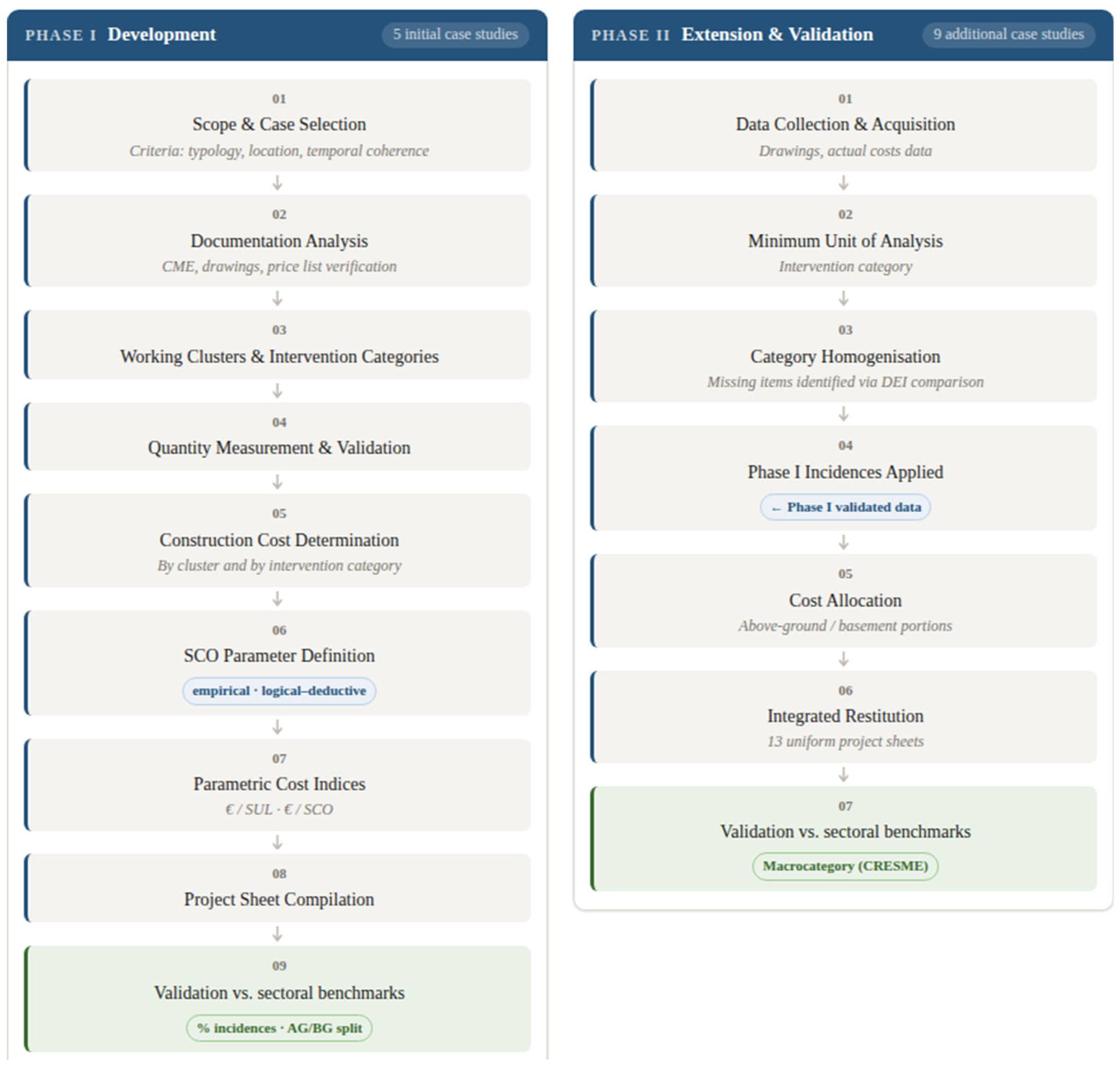
The first phase of the research was conducted on a sample of five residential building interventions (A.1; B.1; C.1; D.1; E.1 described in Section 2.2) and aimed at constructing the foundational structure of the cost assessment model. The phase unfolded through nine sequential analytical steps, each building upon the results of the previous one.

Definition of operational scope and case study selection criteria. Prior to data collection, a preliminary definition of the operational perimeter of the study was established, clarifying the research objectives, the minimum information requirements for case study inclusion, the methodological constraints considered non-negotiable (unit of analysis, scale of application, expected outputs), and the criteria for typological, temporal and locational coherence of the sample. These selection criteria were applied consistently across both phases of the research, ensuring comparability of the full dataset.

Project documentation analysis and cost verification. The initial step consisted of the analytical study of the final-execution level project drawings and the BoQ of the selected case studies. For each case, a structured verification was carried out to assess the congruity of the measurements indicated in the BoQs with those detectable from the project drawings, the correspondence of work item codes and descriptions with those reported in the regional reference price lists, and the reliability of any new unit prices introduced for specific works, verified through a market survey. This preliminary verification phase ensured the documentary reliability of the cost data prior to their systematic processing.

Disaggregation of working clusters and identification of intervention categories. On the basis of the verified documentation, each case study was analysed to identify and disaggregate the working clusters, defined as the spatially and functionally distinct building components that, together with the Gross Built-Up Area (SUL), constitute the total built organism. In parallel, intervention categories were identified corresponding to the technologically homogeneous building components recurring across the different clusters. This dual classification constitutes the backbone of the matrix model adopted for cost organisation, as described in Section 3.

Quantity measurement and validation. For each intervention category and within each working cluster, the quantities were measured and validated against both the project drawings and the values declared in the BoQs in order to ensure internal consistency between the geometric and economic data and to identify any discrepancies requiring correction.

Construction cost determination. The total construction cost was calculated independently for each working cluster and, in parallel, for each intervention category across the entire intervention. This parallel computation allows the cost to be read simultaneously along two axes of the matrix: by spatial component and by technological category.

Unit cost calculation and SCO parameter definition. For each working cluster, the unit construction cost was determined. The percentage contribution of each accessory cluster to the SUL was calculated, providing the basis for the definition of the Homogenised Built Surface (SCO), a normalisation parameter that integrates all surface typologies through homogenisation coefficients reflecting their respective construction cost weights relative to the SUL. The SCO is an original parameter, with no counterpart in existing normative or institutional frameworks for building surface measurement. Its derivation follows an empirical and logical–deductive approach: empirical, because the homogenisation coefficients are not assumed a priori but are calculated directly from the analysis of real construction cost data, project drawings and metric computations of the examined case studies; logical–deductive, because the regularities observed across individual cases are systematically translated into generalisable weighting criteria, applicable to residential projects beyond the specific sample from which they were derived. This dual character—grounded in building practice and extended through structured inference—ensures that the SCO functions as a construction-cost-representative surface denominator, verifiable from actual project documentation and reproducible within analogous analytical contexts. The formulation of the SCO is presented in Section 3.

Parametric construction cost indices. Two parametric indices were calculated for each case study: the cost per unit of SUL, corresponding to the conventional reference parameter, and the cost per unit of SCO, which incorporates the contribution of accessory surfaces through the homogenisation procedure. The dual restitution enables comparison under both the standard and the proposed normalisation criteria.

Project sheet compilation. The final step consisted of the preparation of a structured project sheet for each case study, reporting the total cost, unit cost expressed in both EUR/SUL and EUR/SCO and the percentage contribution of each intervention category. Each sheet further includes a breakdown of the total construction cost between above-ground and below-ground portions and a third subdivision of the total cost by macrocategory: building works, structural works, electrical systems and other mechanical systems. These sheets constitute the primary output of Phase I and serve as the reference instrument for the extension of the framework in Phase II.

Validation vs. sectoral benchmarks. Prior to the extension of the framework to Phase II, the results obtained from Phase I were validated through a systematic comparison with the DEI Prezzario [34] sectoral reference price list. Validation was conducted along two axes: first, the percentage incidences of each intervention category with respect to the total construction cost were compared against the corresponding DEI Prezzario benchmark values; second, the percentage distribution of the total construction cost between the above-ground and below-ground portions was verified against the DEI Prezzario reference ratios. This cross-check served to assess the internal coherence of the proposed framework and to confirm the reliability of the percentage incidences subsequently applied in Phase II. More broadly, the validation of the parametric unit construction costs across both research phases—expressed as EUR/SUL and EUR/SCO—relies on the two principal official Italian reference sources for sectoral cost benchmarking: the DEI Prezzario [34] and CRESME indicators, accessed via the AWN platform [35]. The consistent use of these institutional benchmarks throughout the study ensures that the unit cost indicators produced by the framework are measurable and interpretable within the established national reference system, and that their plausibility can be assessed against widely recognised and regularly updated official data.

2.1.2. Phase II: Extension and Validation of the Framework

The second phase extended the methodological framework to a new sample of nine residential building interventions (A.2; B.2; C.2; D.2; E.2; F.2; G.2; H.2; I.2 described in Section 2.2) all located in the urban transformation areas of the Municipality of Rome. Given the different documentary conditions of this dataset, characterised in several cases by the absence of disaggregated metric computations, the application of the framework required a series of adaptation and harmonisation procedures, described in the following steps.

Data collection and case study acquisition. Nine case studies were acquired, each supported by detailed project documentation (plans, sections, elevations) and actual cost data for overall construction costs. A concurrent assessment of the typological, temporal and locational coherence of the sample was carried out. In this phase, as the economic operators provided actual costs rather than detailed BoQ, it was not possible to disaggregate construction costs at the working cluster level; cost reconstruction was therefore carried out exclusively at the intervention category level. This constraint informed the methodological adaptation described in the subsequent steps.

Definition of the minimum unit of analysis. In response to the documentary limitations identified, the intervention category was adopted as the minimum unit of analysis in place of the working cluster. Categories were adapted and aggregated with reference to the technological composition of the Phase II cases.

Homogenisation and harmonisation of intervention categories. The project cost tables were analysed to identify missing cost items, that is, intervention categories for which no associated cost had been recorded. A homogenisation procedure was applied to reduce the volume of unknown data. Where further aggregation was not possible, as verified by comparison with the DEI Prezzario reference price list, the presence of residual missing percentage incidences was noted and managed through the procedure described in the following step.

Application of Phase I percentage incidences. To ensure methodological continuity between the two phases, taxonomic realignment was performed with respect to the classification adopted in Phase I, with the addition of the cost item hire works and provisional structures. The average percentage incidences of each intervention category, as determined in Phase I, were applied to Phase II aggregations in cases lacking analytical disaggregation, allowing the reconstruction of a complete cost structure while maintaining consistency with the Phase I reference framework.

Cost allocation between residential and basement portions. In Phase I, the allocation of costs between the residential and basement portions was derived automatically from the matrix model. In Phase II, given the aggregated nature of the available data, the allocation was performed by applying the average percentage incidences determined in Phase I, as direct unit cost assignment was not feasible without formal correspondence with the received documentation.

Integrated restitution and project documentation. The concluding step brought together the complete dataset of thirteen case studies, four from Phase I and nine from Phase II, and proceeded to the compilation of uniform project sheets for each intervention, with the objective of rendering results legible, comparable and operationally usable across the full sample.

The overall structure of the research process is summarised in the methodological flowchart presented in Figure 1, which illustrates the sequential steps of the two phases from data collection and cost assessment to validation against official reference sources.

2.2. Case Study Description

The empirical basis of the study consists of a total of thirteen residential building interventions analysed across the two research phases. All cases refer to newly constructed or demolition-and-reconstruction residential buildings, completed or at an advanced construction stage within a timeframe consistent with the objectives of the analysis. The Phase I dataset comprises five residential properties: three located in urban areas of the Municipality of Rome (A.1, B.1, C.1), one in the province of Viterbo (D.1) and one in the province of Naples (E.1). For one of the five cases (E.1), the original construction dates to an earlier period, and a cost update was therefore carried out prior to inclusion in the analysis. The Phase II dataset extends the sample with nine additional interventions (A.2–I.2), all located exclusively within urban transformation areas of the Municipality of Rome.

The selection of case studies for both phases followed a consistent set of criteria ensuring internal comparability and representativeness of contemporary residential building production. Specifically, the selected interventions are as follows: (i) of intervention type new construction (NC) or, alternatively, demolition-and-reconstruction (D/R); (ii) belonging either to the private real-estate sector or to the public/social housing sector (ERP); (iii) located in urban transformation areas as defined by the applicable territorial planning instruments; (iv) characterised by a mid-rise linear residential block typology of about 5 to 7 above-ground storeys and one underground parking level, with an average of two staircase cores and a total of about 20 to 60 apartments per building, comprising a mix of 2-, 3- and 4-room units; (v) characterised by energy class A+, adopted as the uniform reference performance standard for cross-case comparability. The application of these criteria ensures the sample reflects the dominant segment of contemporary residential production in urban transformation contexts. Key typological and economic characteristics of the full dataset are reported as summaries in

Table 1. Typological and locational characteristics of the Phase I case studies.

ID	Type	Period	OMI * Zone	Area	Floors AG + UG **	Units	Quality	Data Source
A.1	NC	2023–2024	E49	Capannelle (RM)	5 + 1	36	High	BoQ
B.1	D/R	2021–2023	D8	Magliana Nuova (RM)	6 + 1	118	Medium	BoQ
C.1	NC	2022–2024	E184	Torrino Mezzocammino (RM)	8 + 1	36	High	BoQ
D.1	D/R	2023–2024	C3	Viterbo (VT)	5 + 1	28	High	FCS ***
E.1	NC	2009–2013	B3	Quarto (NA)	4 + 1	24	High	BoQ

* Real Estate Market Observatory (OMI); **Above Ground (AG), Underground (UG); *** Final Cost Statement (FCS).

,

Table 2. Dimensional and parametric economic data—Phase I case studies.

ID	SUL [m2]	Total Cost [EUR]	Unit Cost per SUL [€/m2]
A.1	2999.34	8,370,210	2790.00
B.1	7722.00	19,151,210	2480.00
C.1	2995.00	9,312,357	3110.00
D.1	2458.98	5,417,250	2205.00
E.1	2805.76	5,051,623	1800.00

,

Table 3. Summary of typological and locational characteristics of Phase II case studies.

ID	Type	Period	OMI Zone	Area	Floors AG + UG	Units	Quality	Data Source
A.2	NC	2021–2024	E40	Castel Giubileo, Rome	5 + 1	48	High	FCS
B.2	NC	2020–2022	E40	Castel Giubileo, Rome	9 + 1	82	High	FCS
C.2	NC	2019–2021	D34	Grotta Perfetta, Rome	7 + 1	36	Medium	FCS
D.2	NC	2020–2023	D34	Grotta Perfetta, Rome	7 + 1	30	Medium	FCS
E.2	D/R	2022–2025	D8	Magliana Nuova, Rome	5 + 0	39	Medium	FCS
F.2	NC	2017	E179	Romanina, Rome	5 + 1	62	Low	FCS
G.2	D/R	2022–2025	D77	Aurelio, Rome	5 + 1	29	High	FCS
H.2	NC	2021–2024	E47	Bufalotta, Rome	5 + 1	54	High	FCS
I.2	NC	2023–2025	E75	Cecchignola, Rome	7 + 1	50	High	FCS

and

Table 4. Summary of dimensional and parametric economic data—Phase II case studies.

ID	SUL [m2]	Total Cost [EUR]	Unit Cost per SUL [€/m2]
A.2	2764.20	7,517,976	2719.77
B.2	3967.00	7,183,573	1810.83
C.2	2176.68	3,509,511	1612.32
D.2	2549.32	4,233,577	1660.67
E.2	2334.00	5,139,000	2201.80
F.2	3959.49	6,172,650	1558.95
G.2	1966.00	5,176,950	2633.24
H.2	4062.50	7,426,401	1828.04
I.2	3923.98	8,985,673	2289.94

.

2.2.1. Phase I Case Studies

Case A.1 is a newly constructed residential building located in the Capannelle urban transformation area, completed in 2024. The building consists of five above-ground residential floors and one underground level accommodating private garages, storage rooms, technical spaces and common services. The load-bearing structure comprises a reinforced concrete frame with shallow foundations; external walls feature thermally insulated cavity masonry with a double perforated brick skin. The ground floor is characterised by a wide front portico providing access to two vertical connection cores, each equipped with one staircase and one lift. Ground-floor units open onto private gardens and loggias; upper floors each accommodate eight apartments with generous private balconies screened by sliding wooden brise-soleil; the top floor hosts six units with large roof terraces. All 36 residential units (49–84 m² net) are served by two bathrooms. The flat roof accommodates a photovoltaic panel system; balcony cornices are clad in ceramic stoneware, and the building envelope is finished in pigmented plaster. External landscaping was fully completed as part of the intervention. The SUL amounts to 2999.34 m² and the total construction cost to EUR 8,370,210 (EUR 2790/m² per SUL). The overall architectural quality is classified as high.

Case B.1 is a demolition-and-reconstruction intervention located in the Magliana peripheral area, completed in 2023, comprising two residential blocks and associated external arrangements: Building A (standard market housing) and Building B (social housing). Both blocks have six above-ground floors and one semi-basement level housing private garages, technical spaces and laundry facilities. Building A features a twin reinforced concrete frame structure with bilateral symmetry, deep pile foundations and a central open courtyard accessible from the ground floor; two vertical connection cores each provide one staircase and two lifts. Ground-floor units (18 total) have private gardens; floors one to five accommodate 20 units per floor with generous private balconies; unit sizes range from 30 to 60 m² net, for 118 total residential units across both buildings. Building B is served by a single central core (one staircase, two lifts), with 10 units at ground level and 11 per upper floor; units are approximately 30–35 m² net (65 units in total). External arrangements include 89 at-grade parking spaces, an ecological waste island and planted areas. The total SUL is 7722.00 m², and the total construction cost was EUR 19,151,210 (EUR 2480/m² per SUL). Building A presents good architectural quality; Building B a medium quality level.

Case C.1 is a newly constructed residential building located in the Torrino Mezzocammino urban transformation area, completed between 2022 and 2024. The building develops over eight above-ground floors—seven residential and one dedicated to shared spaces and technical rooms—plus one underground level for private garages, storage rooms and common services. The load-bearing structure is a reinforced concrete frame with deep pile foundations; external walls feature thermally insulated cavity masonry with a double perforated brick skin. A covered entrance atrium at ground level connects to the single vertical core (one staircase, one lift). The ground floor accommodates one unit with a private covered portico; floors one to seven each accommodate five units with generous private balconies. All 36 residential units (46–92 m² net) are served by two bathrooms. The top floor hosts a laundry room and two rooftop terraces with pergolas; the flat roof accommodates a photovoltaic panel system. Facades are partly clad in high-resistance ceramic stoneware, partly finished in retinated cement plaster with coloured pigments. The SUL amounts to approximately 2995.00 m². This case contributes to the Phase I methodology and incidence derivation but is excluded from the integrated Rome analysis due to the partial availability of economic documentation at the time of data collection.

Case D.1 is a demolition-and-reconstruction intervention located in Viterbo, comprising two twin and specular residential buildings and shared external arrangements. Both buildings develop over five above-ground residential floors and one semi-basement level; the basement is structurally unified across the two bodies but separated by a central structural joint and accommodates private garages. The load-bearing structure is a reinforced concrete frame with raft foundations; external walls feature insulated cavity masonry in thermally insulating blocks with an internal plasterboard skin. Each building is accessed via an entrance hall at ground level, providing access to one staircase and one lift. Ground-floor units (three per building) have private gardens and covered external corridors; floors one to three accommodate three units per floor; the top floor hosts two units with wraparound private terraces partially covered by the flat roof overhang. Unit sizes range from 62 to 117 m² net; total: 14 units per building (28 overall). Balcony parapets are alternately finished in ceramic stoneware and plaster; window reveals are clad in peperino stone and basalt. External arrangements include 49 at-grade parking spaces, an ecological waste island and planted areas. The SUL is 2458.98 m², and the total construction cost was EUR 5,417,250 (EUR 2205/m² per SUL). The case is excluded from the integrated analysis due to its location outside the Municipality of Rome.

Case E.1 is a residential building located in the province of Naples, originally constructed between 2009 and 2013. Given the temporal gap with respect to the reference period of the study, the construction costs were updated to current values prior to inclusion in the Phase I analysis, making this the only case in the dataset processed through a cost-update procedure. The building articulates three structurally independent blocks separated by two seismic joints, each with an independent entrance. The structure is a reinforced concrete frame on a ribbed slab foundation; external walls feature thermally insulated cavity masonry with an outer exposed brick facing and an inner alveolar brick skin. The raised ground floor (elevated approximately 1 m above grade), with a perimeter base clad in lava stone, houses three entrance atria providing access to three vertical connection cores (one staircase and one lift each). From the raised ground floor to the fourth level, each core serves two units per floor, yielding six units per floor and 24 residential units in total (approximately 100–105 m² net each). Every unit is equipped with two loggias and one private balcony; ground-floor units also have a private garden and allotment. The accessible flat roof is reached from all three stairwells. The SUL amounts to 2805.76 m² and the total updated construction cost to EUR 5,051,623 (EUR 1800/m² per SUL). The case is excluded from the integrated analysis due to its location outside the Lazio Region.

2.2.2. Phase II Case Studies

The nine Phase II case studies are all located within the urban transformation areas of the Municipality of Rome, providing the geographic consistency necessary for territorial comparison. Unlike Phase I, the economic documentation available for Phase II consists of cost outturns provided directly by the economic operators, rather than fully disaggregated BoQs. Key characteristics are reported as summaries in Table 3 and Table 4.

Cases A.2 and B.2 are two newly constructed residential buildings developed within the Monti della Breccia urban transformation area at Castel Giubileo, in the northern suburban fringe of Rome. Both complexes share the same structural and morphological approach: two adjacent building blocks of differing heights with a semi-basement level, served by two staircases and two lifts positioned symmetrically relative to the central structural joint. Case A.2 develops on two blocks of five and three above-ground floors respectively, accommodating 48 residential units in total (27 in the taller block: 6 units per floor × 5 levels; 21 in the lower: 7 units per floor × 3 levels), with a SUL of 2764.20 m². Case B.2 develops on two blocks of nine and seven above-ground floors, accommodating 82 residential units (43 in the taller block; 39 in the lower), with a SUL of 3967.00 m². In both cases, the load-bearing structure is a reinforced concrete frame with deep pile foundations; floors are of the mixed reinforced concrete and hollow brick type. Ground-floor units are equipped with private gardens; upper-floor units are served by generous private balconies. The facade is articulated with full-height portals framing planters, aluminium microperforated sheet brise-soleil panels and glass balcony parapets, defining a high architectural quality level in both cases. Construction costs amount to EUR 7,517,975 for A.2 (EUR 2719.77/m² per SUL) and EUR 7,183,573 for B.2 (EUR 1810.83/m² per SUL).

Cases C.2 and D.2 are two newly constructed residential buildings developed in the Grotta Perfetta urban transformation area, in the southern peripheral area of Rome. Both are single-block buildings of approximately 20 m in height, developing over six above-ground residential floors, one technical service floor and one underground level for private garages. Access is provided through a central distribution core (one staircase, one lift). Case C.2 accommodates 36 residential units (6 per floor); the top floor includes a condominium laundry room and a common rooftop terrace with solar panels; ground-floor units have private gardens. Case D.2 accommodates 30 units (5 per floor); ground-floor units are served by generous private terraces; the basement additionally houses bicycle storage and an underground water tank. Both buildings are characterised by generous private balconies at all upper levels, a regular and functional internal distribution scheme and a medium construction quality level. The SUL is 2176.68 m² for C.2, with a unit cost of EUR 1612.32/m² per SUL, and 2549.32 m² for D.2, with a unit cost of EUR 1660.67/m² per SUL.

Case E.2 is a demolition-and-reconstruction intervention located in the Magliana peripheral area, with a construction period of 2022–2025. The intervention consists of a single residential block over five above-ground floors with no underground level. The ground floor has a mixed configuration, housing garages and storage rooms on one side and three residential units on the other; floors one to four each accommodate nine units, for a total of 39 residential units. Ground-floor units are equipped with private gardens; upper-floor units are served by service balconies. The building is served by one staircase and one lift, with a reinforced concrete frame structure on deep foundations. The SUL is 2334.00 m², and the total construction cost was EUR 5,139,000 (EUR 2201.80/m² per SUL). The overall construction quality is classified as medium.

Case F.2 is a newly constructed public residential building located in the Romanina suburban area, with construction commenced in 2017. The complex is articulated in multiple blocks organised around shared spaces and two internal courtyards that promote natural daylighting and ventilation. The building develops over one underground level (private garages and storage rooms), four above-ground residential floors and one additional upper level dedicated to private storage lofts. The distribution system comprises three staircases and three lifts, serving a total of 62 residential units. The exposed brick facade is characteristic of public residential construction standards. The SUL is 3959.49 m², and the total construction cost was EUR 6,172,650 (EUR 1558.95/m² per SUL), consistent with the lower cost level typical of the public housing sector.

Case G.2 is a demolition-and-reconstruction intervention located in the Aurelio/Val Cannuta peripheral area, with a construction period of 2022–2025. The intervention consists of a single residential block over five above-ground floors and one semi-basement level, plus an accessible flat roof. The semi-basement accommodates three residential units with dedicated private gardens, in addition to storage rooms and technical spaces. Access is provided through a single vertical distribution core (one staircase, one lift) serving all levels. The total residential count is 29 units. The accessible rooftop level provides private terraces for the top-floor units and accommodates a photovoltaic system; shaded at-grade parking spaces are included in the external arrangements. High-quality finishes and materials contribute to an elevated construction quality level. The SUL is 1966.00 m², and the total construction cost was EUR 5,176,950 (EUR 2633.24/m² per SUL).

Case H.2 is a newly constructed residential complex located in the Bufalotta urban transformation area, with a construction period of 2021–2024. The complex consists of two adjacent residential buildings on a sloping plot, whose variable terrain gradient determines different ground-floor levels for the two buildings; the northern block is further articulated by an internal structural joint. Both buildings develop over five above-ground floors with one shared underground level housing private garages, storage rooms and technical spaces. The distribution system comprises three staircases and three lifts. The load-bearing structure is a reinforced concrete frame with shallow foundations. The complex accommodates 54 residential units in total, all equipped with service balconies. Landscaped external areas integrate the complex with its surroundings. High-quality materials and finishes, together with an articulated spatial composition responsive to site conditions, define the overall high construction quality level. The SUL is 4062.50 m², and the total construction cost was EUR 7,426,401 (EUR 1828.04/m² per SUL).

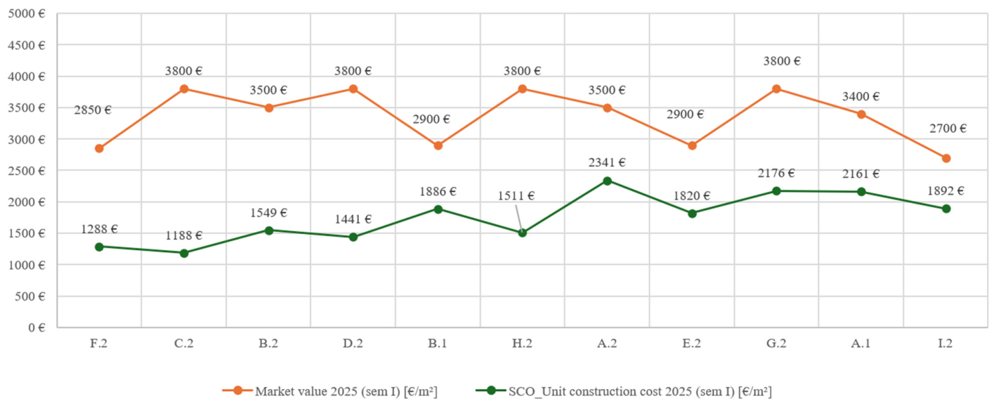
Case I.2 is a newly constructed mixed-use building located in the Cecchignola Ovest–Tor Pagnotta urban transformation area, with a construction period of 2023–2025. The building develops over seven above-ground floors and one underground level (private garages, storage rooms and common services). The ground floor accommodates six commercial units; residential uses begin on the first floor, including 11 units under a regulated rent arrangement. The planimetric configuration is organised around two internal courtyards that promote natural daylighting and ventilation. Ten apartments are distributed per floor, for a total of 50 residential units, all equipped with generous private balconies. The distribution system comprises two staircases and two lifts. The load-bearing structure is a reinforced concrete frame with deep foundations. The roof level houses have technical spaces, a condominium laundry room and photovoltaic/solar-thermal installations. Quality materials, advanced technologies and high-quality finishes define the overall elevated construction quality level. The SUL is 3923.98 m², and the total construction cost was EUR 8,985,673 (EUR 2289.94/m² per SUL). The OMI market value [36] in the microzone (EUR 2700/m²) is discussed in the territorial analysis presented in Section 3.2.

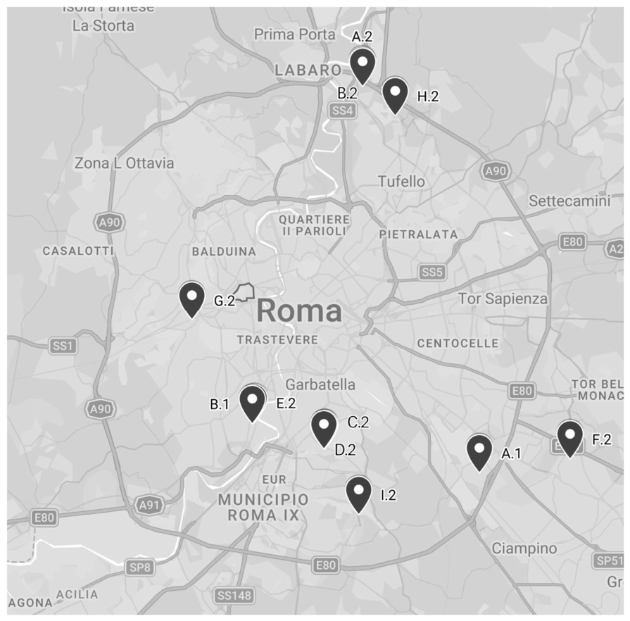
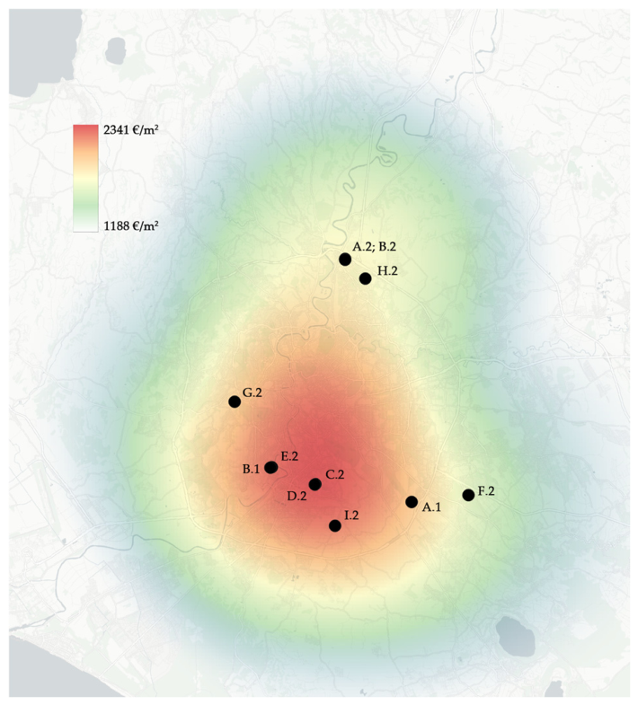
The geographic distribution of the eleven Rome-based case studies covers the principal urban transformation quadrants of the city (Figure 2): the northern suburban fringe (A.2, B.2), the southern peripheral areas (C.2, D.2; I.2), the eastern and southeastern suburban belt (A.1; H.2; F.2) and the western and southwestern peripheral ring (B.1, E.2; G.2). This spatial diversity supports the GIS-based territorial analysis of updated parametric construction costs described in Section 3.2.

For the integrated analysis presented in Section 3.2, the working dataset consists of the eleven Rome-based case studies: cases A.1 and B.1 from Phase I and all nine cases (A.2–I.2) from Phase II. Cases C.1, D.1 and E.1 are retained for the derivation of Phase I reference incidence percentages but excluded from the integrated territorial analysis due to documentary limitations (C.1) or geographic scope (D.1, E.1).

3. Results

This section presents the outcomes of the two-phase research project, structured according to the sequential logic of the methodological framework described in Section 2. Phase I results are grounded in detailed BoQ from five case studies; Phase II results extend and update the model through parametric data collected directly from nine additional economic operators active in the Municipality of Rome. Both phases converge on a set of operative tools—interactive project sheets, a territorial GIS map and synthetic unit cost indicators—designed to support practitioners in preliminary cost estimation.

3.1. Phase I Results

The logical-operative process developed requires a preliminary step: clarifying what is meant by construction cost. This term encompasses the technical cost of construction (materials, labour, plant hire and transport) and the “indirect” items (ordinarily equal to 26.5% of the technical construction cost), comprising general overheads and contractor’s profit [2]. Excluded from the construction cost are the following: (a) land cost; (b) professional fees; (c) urbanisation charges; (d) utility connection fees. For the case studies analysed, reference is made to costs at the design estimate stage, with the exclusion of items related to temporary works (scaffolding) and safety charges.

3.1.1. Matrix Model

In order to define a baseline parametric construction cost for the selected case studies, a matrix model was developed following the methodological approach defined in Section 2. The model provides a systematic framework for representing and managing complex relationships among cost data, making it possible to organise large quantities of information in a clear and readable tabular form, thereby facilitating the interpretation and analysis of interdependencies between different building components. Through the following system architecture, it is possible to examine and quantify the relationships among the various variables, supporting comparative analyses and scenario simulations.

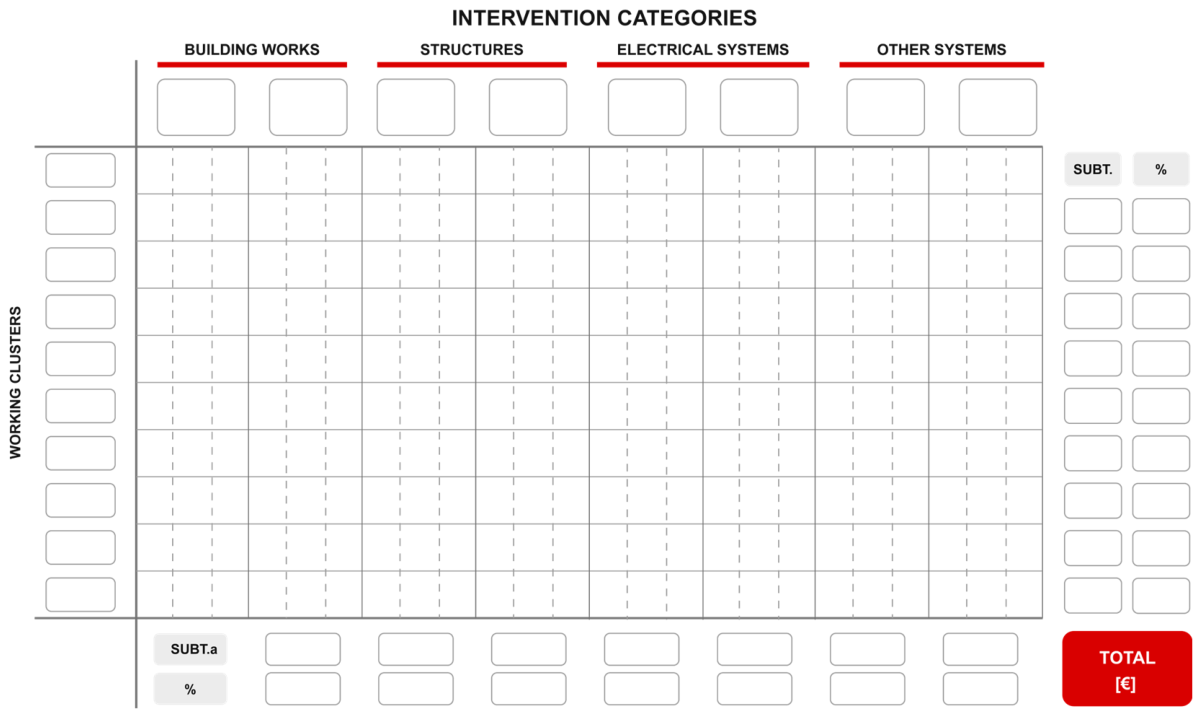
Furthermore, the modular structure allows data to be easily updated and modified, rendering the tool suitable for continuous monitoring and economic review throughout all design phases. The reference matrix was constructed based on a dual classification of the items that contribute to defining the total construction cost through a hierarchical Work Breakdown Structure (WBS) approach. Within this framework, the total construction cost is decomposed top-down along two independent dimensions: a spatial dimension (working clusters) and a technological dimension (intervention categories) (Figure 3).

The first classification, “working clusters”, considers the building components that, together with the SUL, constitute the SCO. This classification identifies the working clusters listed in

Table 5. Working clusters.

External works and/or porticoes	Private gardens and allotments
Lift shafts and lifts	Roofing/flat roof
Loggias, balconies and terraces	Semi-basement level
Plant rooms and technical enclosures	Stairwells and entrance halls
Gross Built-Up Area (SUL)

.

The second classification, “intervention categories”, considers the disaggregation of the total intervention into homogeneous building components from a technological standpoint. The categorisation adopted during the computation stage was taken into account. This classification identifies the intervention categories listed in

Table 6. Classification of intervention categories.

Carpentry and joinery works	Masonry works
Earthworks	Painting and decorating works
Electrical installation	Photovoltaic systems
External windows and doors	Plasterboard works
Fire-protection system	Plastering and rendering
Floor screeds	Prefabricated elements
Flooring and wall cladding	Reinforced-concrete and clay-concrete composite works
Foundations	Retaining walls
Industrial flooring	Sewerage, water-pumping and gas-connection systems
Infill walls	Steel, aluminium and sheet-metal works
Internal dividing elements	Stonework
Internal doors and frames	Structural joints
Internal partition walls	Thermal and acoustic insulation
Landscaping and urban furnishings	Water supply, sanitary and heating systems
Lift installation	Waterproofing

.

In identifying the intervention categories, a further classification by macrocategories was adopted, comprising the following: building/civil works, structures, electrical systems and other systems.

Table 7. Mapping of intervention categories to macrocategories.

Macrocategories	Intervention Categories
Building/civil works	Carpentry and joinery works; Painting and decorating works; External windows and doors; Plasterboard works; Plastering and rendering; Floor screeds; Prefabricated elements; Flooring and wall cladding; Industrial flooring; Infill walls; Steel, aluminium and sheet-metal works; Internal dividing elements; Stonework; Internal doors and frames; Internal partition walls; Thermal and acoustic insulation; Landscaping and urban furnishings; Waterproofing.
Structures	Masonry works; Earthworks; Reinforced-concrete and clay-concrete composite works; Foundations; Retaining walls; Structural joints.
Electrical systems	Electrical installations
Other systems	Photovoltaic systems; Fire-protection system; Sewerage, water-pumping and gas-connection systems; Water-supply, sanitary and heating systems; Lift installation.

maps each of the 30 intervention categories to its corresponding macrocategory, providing the reference taxonomy for the cost analysis presented in the following sections.

Once the matrix was constructed, the data were placed by associating each BoQ item with the corresponding reference category, according to the working cluster to which it belonged. For each item, values for quantity, unit cost and total cost were recorded.

A first analysis involved the computation of the partial totals for each cluster, enabling, once the surface area was established, the derivation of the corresponding unit costs and the percentage incidences relative to the SUL unit cost. At the same time, the partial totals for each intervention category and their percentage incidences relative to the total construction cost were computed.

The percentage contribution of each cluster contributes to the definition of the SCO parameter. The need to define this parameter arises from the requirement to account for accessory surfaces (such as stairwells, lifts, terraces, gardens, etc.) that, while not directly included in the SUL, significantly affect the overall construction cost of the building. The SCO is defined as the sum of the SUL and the surfaces of the accessory working clusters—stairwells/entrance halls (VSA), lift shafts (VCA), semi-basement level (PS), etc.—appropriately homogenised on the basis of their respective incidence coefficients (IC_Vsa, IC_Vca, IC_ps, etc.), expressing the unit cost of each cluster relative to that of the main residential area (Equation (1)). These incidence coefficients are weighted quantities: each is computed as the ratio of the construction cost attributable to the given cluster—encompassing all intervention categories falling within that cluster—to the total construction cost of the entire building, thereby ensuring that the homogenisation reflects the actual economic contribution of each accessory surface rather than a purely geometric approximation.

$$\mathrm{S}\mathrm{C}\mathrm{O}=\mathrm{S}\mathrm{U}\mathrm{L}+\left(\mathrm{V}\mathrm{S}\mathrm{A}\times {\mathrm{I}\mathrm{C}}_{{\mathrm{V}}_{\mathrm{s}\mathrm{a}}}\right)+\left(\mathrm{V}\mathrm{C}\mathrm{A}\times {\mathrm{I}\mathrm{C}}_{{\mathrm{V}\mathrm{C}}_{\mathrm{a}}}\right)+\left(\dots \right)+\left(\mathrm{P}\mathrm{S}\times {\mathrm{I}\mathrm{C}}_{\mathrm{p}\mathrm{s}}\right).$$

(1)

In this way, a synthetic measure of the overall economic impact of the various surfaces contributing to the building stock to be realised is obtained.

3.1.2. Working Cluster Analysis

A sample of five newly constructed residential buildings was analysed, completed between 2023 and 2024, with the exception of one case study for which a cost update was carried out. The analysis was conducted on buildings located throughout the Italian territory: among the properties identified, three are situated within urban transformation areas of the city of Rome (Lazio), one is located in the province of Viterbo (Lazio) and the fifth case study is situated in the province of Naples (Campania). All case studies were built on plots characterised by predominantly flat terrain.

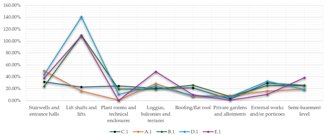
A.1 (Rome, 2023–2024). As reported in

Table 8. Parametric cost and homogenisation coefficient synthesis sheet—A.1.

	Surface Area [m2]	Total Cost [EUR]	Unit Cost [EUR/m2]	Cluster Unit–Cost Incidence vs. SUL Unit Cost [%]	Cluster Cost Incidence vs. SUL Cost [%]	Cluster Cost Incidence vs. Total Construction Cost [%]
Stairwells and entrance halls	313.32	324,564.72	1035.89	49.83%	5.21%	3.88%
Lift shafts and lifts	66.24	21,853.73	329.92	15.87%	0.35%	0.26%
Plant rooms and technical enclosures	27.20	460.55	16.93	0.81%	0.01%	0.01%
Loggias, balconies and terraces	1211.20	717,535.01	592.42	28.50%	11.51%	8.57%
Roofing/flat roof	641.87	98,347.32	153.22	7.37%	1.58%	1.17%
Private gardens and allotments	169.81	29,613.69	174.39	8.39%	0.47%	0.35%
External works and/or porticoes	613.00	205,709.36	335.58	16.14%	3.30%	2.46%
Gross Built-Up Area (SUL)	2999.34	6,235,220.21	2078.86	-	-	74.49%
Semi-basement level	1827.97	736,905.68	403.13	19.39%	11.82%	8.80%
Total construction cost		8,370,210.27
SUL	2999.34		2790.00
SCO	4026.34		2080.00
Difference [%]			25.45%

, the total construction cost amounts to EUR 8,370,210.27. Considering a SUL of 2999.34 m², the unit cost per SUL is estimated at EUR 2790/m². Considering only the above-ground volumes, the unit cost per SUL is EUR 2545/m². The unit cost incidences of the individual working clusters show a generally heterogeneous pattern, with an average value of 18.29%, a minimum of 0.81% for technical rooms and a maximum of 49.83% for stairwells and entrance halls. Based on the percentage weight of each cluster, the SCO was computed at 4026.34 m². The unit cost per SCO is EUR 2080/m². The unit cost relative to the total constructed volume is EUR 467.68/m³; considering only the above-ground constructed volume of 15,760.00 m³, the unit cost is EUR 531.10/m³.

B.1 (Rome, 2021–2023). As reported in

Table 9. Parametric cost and homogenisation coefficient synthesis sheet—B.1.

	Surface Area [m2]	Total Cost [EUR]	Unit Cost [EUR/m2]	Cluster Unit–Cost Incidence vs. SUL Unit Cost [%]	Cluster Cost Incidence vs. SUL Cost [%]	Cluster Cost Incidence vs. Total Construction Cost [%]
Stairwells and entrance halls	1362.81	585,863.45	429.89	23.96%	4.23%	3.06%
Lift shafts and lifts	176.47	347,662.20	1970.09	109.81%	2.51%	1.82%
Plant rooms and technical enclosures	366.77	126,610.53	345.20	19.24%	0.91%	0.66%
Loggias, balconies and terraces	4018.62	1,395,565.52	347.27	19.36%	10.07%	7.29%
Roofing/flat roof	923.43	429,816.33	465.46	25.94%	3.10%	2.24%
Private gardens and allotments	1426.67	171,207.14	120.00	6.69%	1.24%	0.89%
External works and/or porticoes	1280.85	582,356.97	454.66	25.34%	4.20%	3.04%
Gross Built-Up Area (SUL)	7721.99	13,853,627.63	1794.05	-	-	72.34%
Semi-basement level	3670.20	1,658,500.81	451.88	25.19%	11.97%	8.66%
Total construction cost		19,151,210.58
SUL	7721.99		2480.00
SCO	10,674.85		1795.00
Difference [%]			27.62%

, the total construction cost amounts to EUR 19,151,210.58. Considering an SUL of 7721.99 m², the unit cost per SUL is EUR 2480/m². Considering only the above-ground volumes, the unit cost per SUL is EUR 2265.00/m². The unit cost incidences of the individual working clusters show a sufficiently homogeneous pattern: the average coefficient is 31.94%, with a minimum of 6.69% for private gardens/allotments and a maximum of 109.81% for lift shafts. Based on the percentage weight of each cluster, the SCO was computed at 10,674.85 m². The unit cost per SCO is EUR 1795/m². The unit cost of the total constructed volume is EUR 515.88/m³; considering the above-ground constructed volume of 50,898.00 m³, the unit cost is EUR 376.27/m³.

C.1 (Rome, 2021–2023). As reported in

Table 10. Parametric cost and homogenisation coefficient synthesis sheet—C.1.

	Surface Area [m2]	Total Cost [EUR]	Unit Cost [EUR/m2]	Cluster Unit–Cost Incidence vs. SUL Unit Cost [%]	Cluster Cost Incidence vs. SUL Cost [%]	Cluster Cost Incidence vs. Total Construction Cost [%]
Stairwells and entrance halls	492.91	370,203.81	751.06	31.54%	5.19%	3.98%
Lift shafts and lifts	48.62	26,324.68	541.47	22.74%	0.37%	0.28%
Plant rooms and technical enclosures	91.37	53,120.87	581.38	24.42%	0.74%	0.57%
Loggias, balconies and terraces	977.56	477,009.95	487.96	20.49%	6.69%	5.12%
Roofing/flat roof	223.24	113,547.47	508.63	21.36%	1.59%	1.22%
Private gardens and allotments	100.64	5418.53	53.84	2.26%	0.08%	0.06%
External works and/or porticoes	588.13	412,332.29	701.09	29.45%	5.78%	4.43%
Gross Built-Up Area (SUL)	2995.07	7,131,133.49	2380.96	-	-	76.58%
Semi-basement level	1188.28	723,266.66	608.67	25.56%	10.14%	7.77%
Total construction cost		9,312,357.75
SUL	2995.07		3110.00
SCO	3911.18		2380.00
Difference [%]			23.47%

, the total construction cost amounts to EUR 9,312,357.75. Considering a SUL of 2995.07 m², a unit cost per SUL of EUR 3110.00/m² is obtained. Considering only the above-ground volumes (i.e., excluding the basement level), the unit cost per SUL is EUR 2870.00/m². The unit cost incidences of the individual working clusters show a sufficiently homogeneous pattern: the average weight of the clusters is 22.23%, with a minimum coefficient of 2.26% for private gardens/allotments and a maximum of 31.54% for stairwells and entrance halls. Based on the percentage weight of each working cluster, the SCO was computed at 3911.18 m². The unit cost per SCO is EUR 2380/m². The unit cost per cubic metre of total constructed volume is EUR 442.89/m³; considering only the above-ground constructed volume of 18,386.00 m³, the unit cost is EUR 506.49/m³.

D.1 (Viterbo, 2023–2024). As reported in

Table 11. Parametric cost and homogenisation coefficient synthesis sheet—D.1.

	Surface Area [m2]	Total Cost [EUR]	Unit Cost [EUR/m2]	Cluster Unit–Cost Incidence vs. SUL Unit Cost [%]	Cluster Cost Incidence vs. SUL Cost [%]	Cluster Cost Incidence vs. Total Construction Cost [%]
Stairwells and entrance halls	353.28	223,939.57	633.89	43.83%	6.30%	4.13%
Lift shafts and lifts	42.30	85,996.07	2033.00	140.56%	2.42%	1.59%
Plant rooms and technical enclosures	40.00	6160.00	154.00	10.65%	0.17%	0.11%
Loggias, balconies and terraces	868.06	305,983.55	352.49	24.37%	8.60%	5.65%
Roofing/flat roof	870.00	106,093.37	121.95	8.43%	2.98%	1.96%
Private gardens and allotments	1385.88	130,512.69	94.17	6.51%	3.67%	2.41%
External works and/or porticoes	1058.60	497,029.35	469.52	32.46%	13.97%	9.17%
Gross Built-Up Area (SUL)	2458.98	3,556,600.01	1446.37	-	-	65.65%
Semi-basement level	1867.70	504,936.10	270.35	18.69%	14.20%	9.32%
Total construction cost		5,417,250.71
SUL	2458.98		2205.00
SCO	3745.41		1445.00
Difference [%]			34.47%

, the total construction cost amounts to EUR 5,417,250.71. Considering a SUL of 2458.98 m², the unit cost per SUL is EUR 2205/m². Considering only the above-ground volumes, the unit cost per SUL is EUR 2000/m². The unit cost incidences of the individual working clusters show a sufficiently homogeneous pattern: the average contribution is 35.69%, with a minimum of 6.51% for private gardens/allotments and a maximum of 140.56% for lift shafts. Based on the percentage weight of each cluster, the SCO was computed at 3745.41 m². The unit cost per SCO is EUR 1445/m². The unit cost of the total constructed volume amounts to EUR 290.77/m³; considering only the above-ground constructed volume of 11,721.27 m³, the unit cost is EUR 462.17/m³.

E.1 (Naples, 2009–2013, updated). As reported in

Table 12. Parametric cost and homogenisation coefficient synthesis sheet—E.1.

	Surface Area [m2]	Total Cost [EUR]	Unit Cost [EUR/m2]	Cluster Unit–Cost Incidence vs. SUL Unit Cost [%]	Cluster Cost Incidence vs. SUL Cost [%]	Cluster Cost Incidence vs. Total Construction Cost [%]
Stairwells and entrance halls	422.25	202,227.06	478.93	37.72%	5.68%	4.00%
Lift shafts and lifts	81.24	112,392.38	1383.46	108.96%	3.15%	2.22%
Plant rooms and technical enclosures	-	-	-	-	-	-
Loggias, balconies and terraces	497.37	307,918.00	619.09	48.76%	8.64%	6.10%
Roofing/flat roof	788.94	97,900.64	124.09	9.77%	2.75%	1.94%
Private gardens and allotments	60.00	467.08	7.78	0.61%	0.01%	0.01%
External works and/or porticoes	1733.29	229,598.52	132.46	10.43%	6.44%	4.55%
Gross Built-Up Area (SUL)	2805.76	3,562,454.72	1269.69	-	-	70.52%
Semi-basement level	1105.37	538,665.20	487.32	38.38%	15.12%	10.66%
Total construction cost		5,051,623.59
SUL	2805.76		1800.00
SCO	3978.62		1270.00
Difference [%]			29.44%

, the total construction cost amounts to EUR 5,051,623.59. Considering an SUL of 2805.76 m², the unit cost per SUL is EUR 1800/m². Considering only the above-ground volumes, the unit cost per SUL is EUR 1610/m². The unit cost incidences of the individual working clusters show a sufficiently homogeneous pattern, with an average weight of 36.38%, a minimum of 0.61% for private gardens/allotments and a maximum of 108.96% for lift shafts. Based on the percentage weight of each cluster, the SCO was computed at 3978.62 m². The unit cost per SCO is EUR 1270/m². The unit cost relative to the total constructed volume is EUR 472.73/m³; considering the above-ground constructed volume of 12,186.54 m³, the unit cost is EUR 414.52/m³.

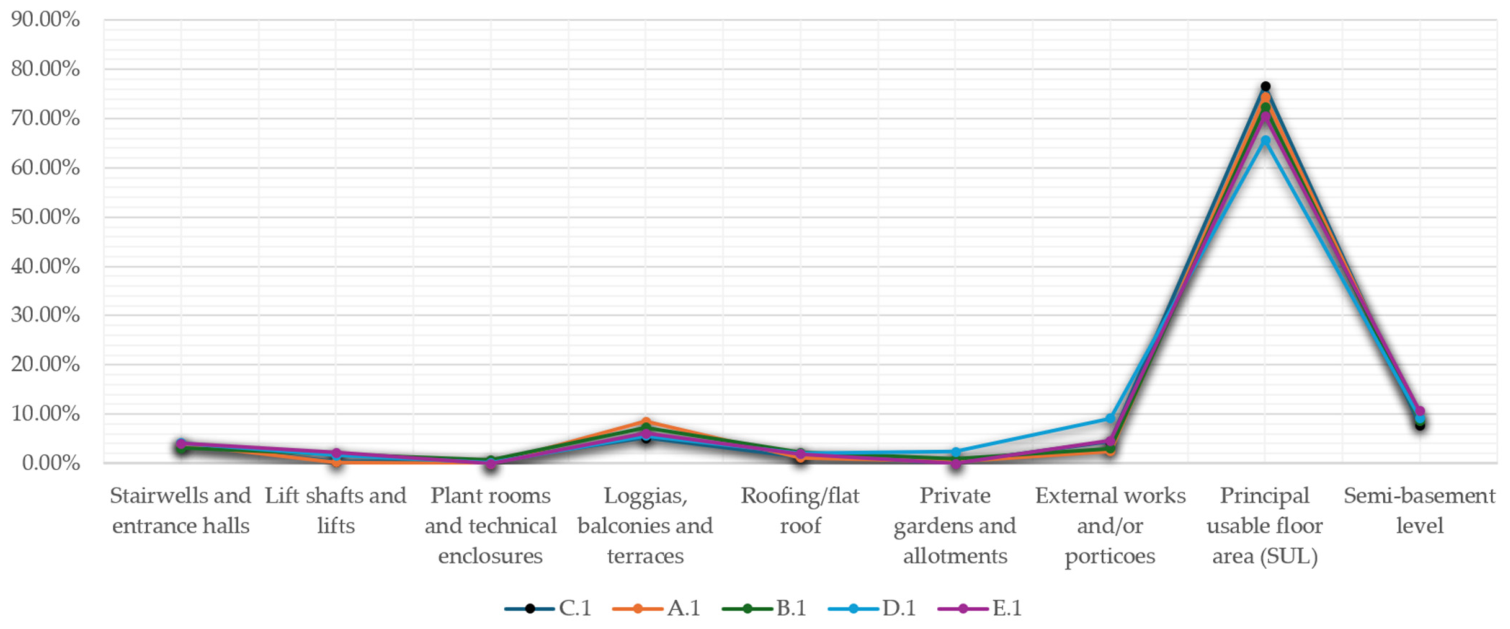
The analysis of unit costs and their incidences for working clusters, referring to the averages of the Rome case studies (

Table 13. Average parametric cost and homogenisation coefficient synthesis—Rome case studies.

	Unit Cost [EUR/m2]	Cluster Unit–Cost Incidence vs. SUL Unit Cost [%]	Cluster Cost Incidence vs. SUL Cost [%]	Cluster Cost Incidence vs. Total Construction Cost [%]
Stairwells and entrance halls		35.11%	4.88%	3.64%
Lift shafts and lifts		49.47%	1.08%	0.79%
Plant rooms and technical enclosures		14.82%	0.56%	0.41%
Loggias, balconies and terraces		22.78%	9.42%	6.99%
Roofing/flat roof		18.23%	2.09%	1.55%
Private gardens and allotments		5.78%	0.60%	0.44%
External works and/or porticoes		23.64%	4.43%	3.31%
Gross Built-Up Area (SUL)		-	-	74.47%
Semi-basement level		23.38%	11.31%	8.41%
SUL	2795.00
SCO	2085.00
Difference [%]	25.51%

), highlights some significant dynamics in cost distribution. The SUL represents the predominant item, accounting for 74.47% of the total cost of the intervention, thereby confirming its decisive weight in defining construction costs. Among the accessory clusters, “lift shafts” and “stairwells and entrance halls” register incidences of 49.47% and 35.11%, respectively, relative to the SUL unit cost, demonstrating the high unit cost of these components, while their contribution to the total cost of the intervention is lower (0.79% and 3.64%, respectively). The “loggias, balconies and terraces” cluster is also characterised by a non-negligible incidence, with a unit cost of 22.78% relative to the SUL and a weight of 6.99% on the total cost. The “semi-basement” cluster, with an incidence of 11.31% relative to the SUL, represents a further relevant element. Finally, the comparison between the SUL unit cost (EUR 2795/m²) and the SCO unit cost (EUR 2085/m²) yields a difference of 25.51%, highlighting how accessory surfaces significantly affect the overall construction cost. Additionally, considering only the above-ground volumes, the average unit cost per SUL is EUR 2560/m².

The analysis of average unit costs, extended to all case studies including those located in the province of Viterbo and at Quarto (NA), allows the perspective on construction cost distribution by cluster to be broadened. Compared to the Rome averages alone, some significant variations emerge. The SUL is confirmed as the primary cost item, with an incidence of 71.92% of the total intervention, slightly lower than the value found in the Rome cases (74.47%). The accessory clusters, however, show a different relative incidence: in particular, the unit cost of “lift shafts” is considerably higher (79.59% relative to the SUL, against 49.47% of the Rome average), indicating a greater economic impact of this component in the extra-urban contexts considered. The “loggias, balconies and terraces” cluster presents a unit cost higher than the Rome average (28.30% vs. 22.78%), with a correspondingly greater incidence on the total cost (6.99% vs. 6.55%). The “semi-basement” registers a higher incidence on the total cost (12.65% vs. 11.31% for the Rome average). The SUL unit cost, at EUR 2475/m², is lower than the Rome average (EUR 2795/m²), as is the SCO unit cost (EUR 1795/m² vs. EUR 2085/m²), yielding an overall percentage difference of 28.09%, slightly higher than for the Rome cases alone (25.51%). Considering only the above-ground volumes, the average SUL unit cost for the entire sample is EUR 2260/m².

These results highlight how geographical location and territorial specificities can significantly influence the distribution of construction costs, determining the need for a calibrated assessment of the peculiarities of each project and the context in which it is located. Considering the unit cost referred to building volume, a mean unit cost for the entire case study set of EUR 458.11/m³ is obtained for the above-ground volume, while for the total volume the mean value is EUR 437.99/m³.

3.1.3. Intervention Categories

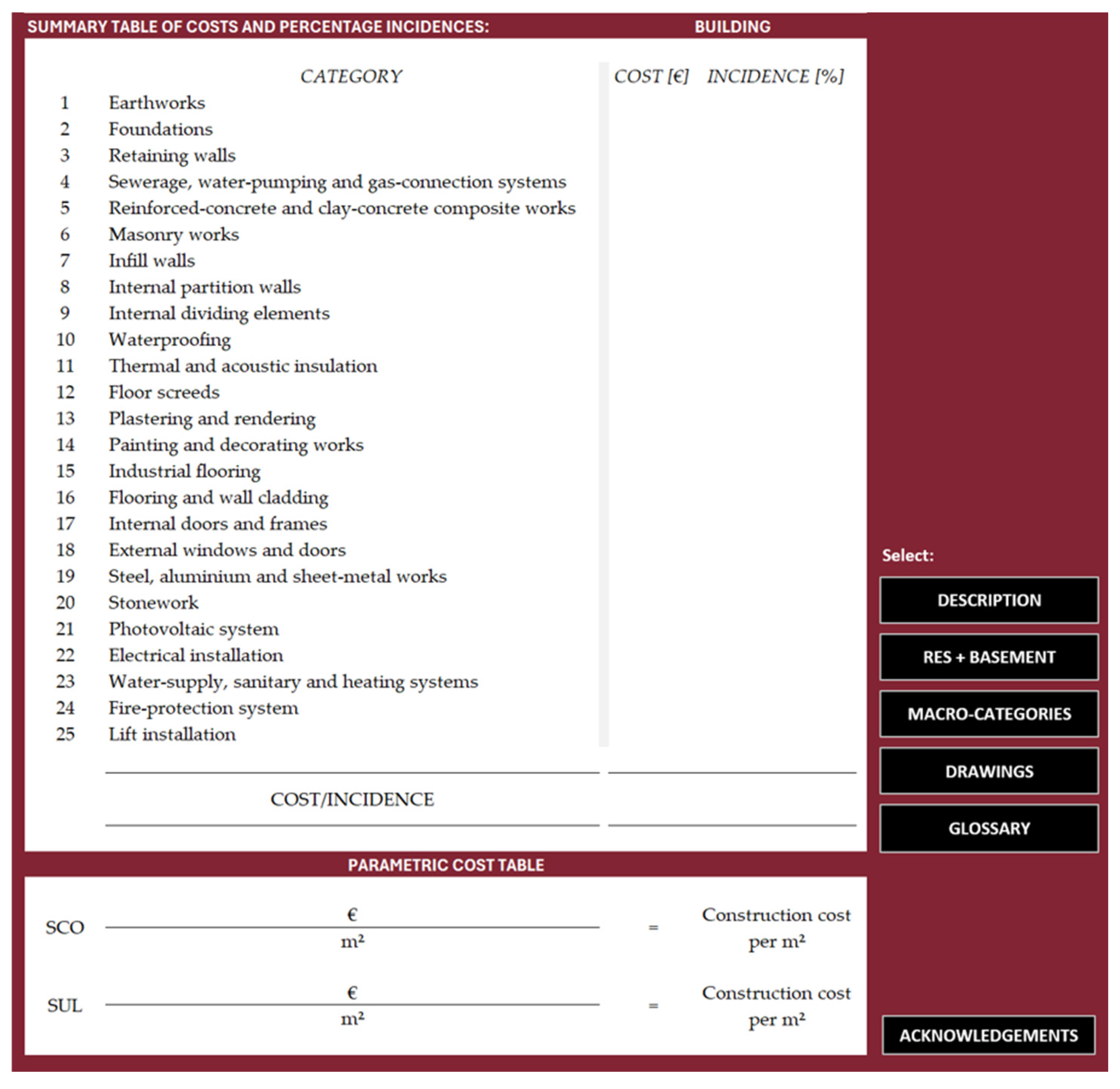
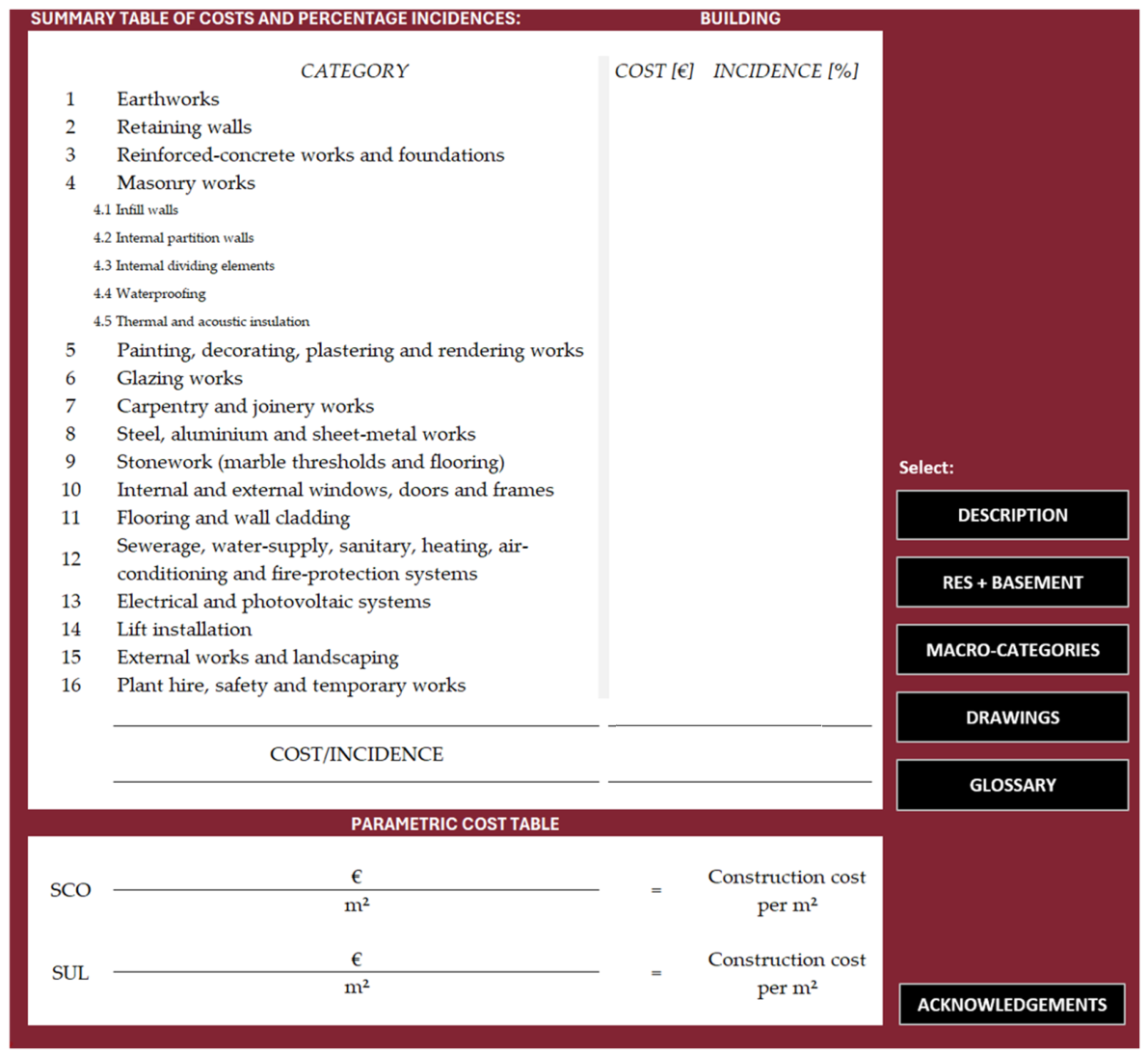
In order to achieve a complete characterisation of the construction costs of the intervention—enabling the parties involved in its realisation (contracting authority, contractor, designer, site supervisor, inspector, etc.) to rapidly identify the contribution of the expenditure items (categories)—interactive project sheets were prepared for each case study. These sheets summarise the following: (i) the intervention categories with their corresponding construction costs and percentage incidences on the total construction cost; (ii) the unit construction cost per SUL; (iii) the unit construction cost per SCO; (iv) the items referred to in point (i), differentiated for above-ground floors and basement level; (v) the disaggregation of the project into macrocategories, specifying the corresponding total costs and percentage incidences on the total construction cost. In addition, each sheet is accompanied by project drawings and an appropriate description of technological and locational aspects, as well as a glossary to support the understanding of acronyms and the various terms defining the information matrix. By way of example, Figure 4 shows an extract from a project sheet.

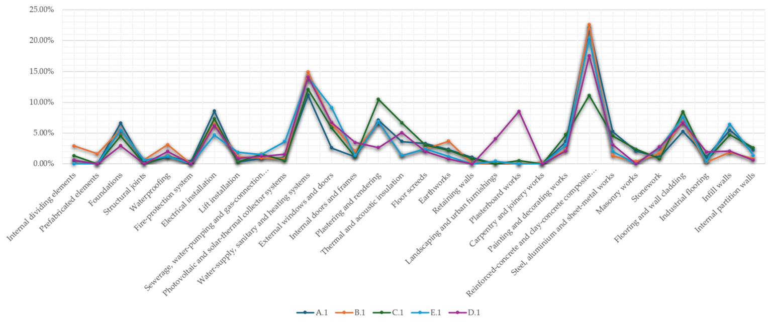
Furthermore, in order to delineate a comparative framework among the different case studies, an analysis of the percentage incidences of each intervention category on the total construction cost was carried out. This comparison, reported in

Table 14. Analysis of the percentage incidences of each intervention category on the total construction cost.

Intervention Categories	A.1	B.1	C.1	E.1	D.1	Overall Average
Carpentry and joinery works	0.00%	0.26%	0.00%	0.00%	0.00%	0.05%
Earthworks	2.34%	3.69%	2.20%	1.22%	0.80%	2.05%
Electrical installation	8.56%	6.55%	7.33%	4.68%	6.25%	6.67%
External windows and doors	2.59%	6.56%	5.85%	9.13%	6.70%	6.17%
Fire-protection system	0.42%	0.00%	0.14%	0.05%	0.00%	0.12%
Floor screeds	3.30%	2.47%	3.05%	2.44%	2.00%	2.65%
Flooring and wall cladding	5.27%	6.96%	8.48%	7.58%	6.71%	7.00%
Foundations	6.62%	5.61%	4.55%	5.50%	2.95%	5.05%
Industrial flooring	1.16%	0.28%	0.60%	0.42%	1.94%	0.88%
Infill walls	5.46%	1.88%	4.72%	6.45%	2.08%	4.12%
Internal dividing elements	0.53%	2.92%	1.34%	0.00%	0.62%	1.08%
Internal doors and frames	1.13%	2.02%	1.17%	1.36%	3.49%	1.84%
Internal partition walls	2.26%	0.85%	2.63%	1.40%	0.63%	1.55%
Landscaping and urban furnishings	0.00%	0.16%	0.00%	0.45%	4.06%	0.94%
Lift installation	0.30%	1.16%	0.29%	1.89%	0.93%	0.91%
Masonry works	2.06%	0.40%	2.39%	0.00%	0.00%	0.97%
Painting and decorating works	3.63%	2.27%	4.75%	3.08%	2.14%	3.17%
Photovoltaic system	0.98%	0.84%	0.53%	3.64%	1.58%	1.51%
Plasterboard works	0.00%	0.00%	0.54%	0.00%	8.52%	1.81%
Plastering and rendering	7.09%	6.81%	10.47%	6.83%	2.64%	6.77%
Prefabricated elements	0.00%	1.65%	0.00%	0.00%	0.00%	0.33%
Reinforced-concrete and clay-concrete composite works	22.09%	22.60%	11.11%	20.38%	17.54%	18.74%
Retaining walls	1.04%	0.00%	0.86%	0.00%	0.00%	0.38%
Sewerage, water-pumping and gas-connection systems	0.92%	0.95%	1.57%	1.51%	1.23%	1.24%
Steel, aluminium and sheet-metal works	5.24%	1.31%	4.57%	2.03%	3.13%	3.26%
Stonework	1.07%	1.73%	0.82%	2.66%	2.78%	1.81%
Structural joints	0.00%	0.67%	0.00%	0.62%	0.00%	0.26%
Thermal and acoustic insulation	3.65%	1.37%	6.67%	1.35%	5.10%	3.63%
Waterproofing	1.16%	3.11%	1.28%	1.23%	2.03%	1.76%
Water supply, sanitary and heating systems	11.13%	14.93%	12.09%	14.11%	14.12%	13.28%

, enables the assessment of the distributional homogeneity of items and allows the identification of recurring trends, providing an analytical view of the economic dynamics characterising the building processes under study.

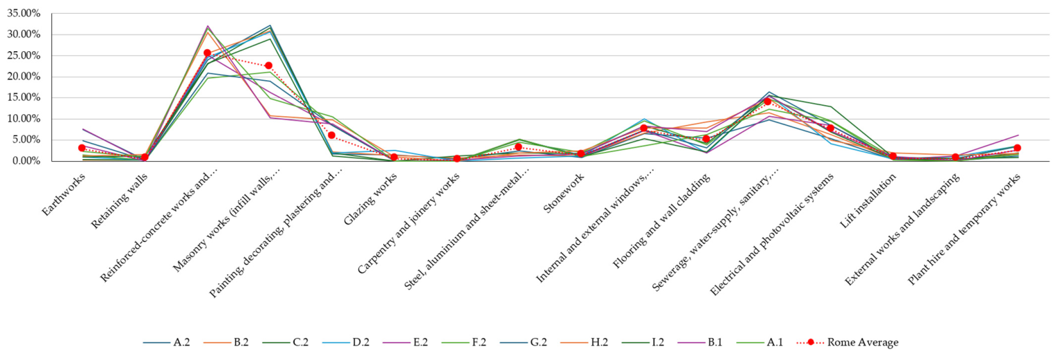
From the analysis of the data reported in Table 14, it emerges that the intervention categories with the most significant impact on the total construction cost are “reinforced concrete and laterocement structures”, which represent the predominant share with an average incidence of 18.74%, followed by “Water-supply, sanitary and heating systems“ accounting for 13.28% of the total cost. Another significant item is “electrical systems”, with an average incidence of 6.67%. Among other intervention categories, “flooring and cladding” (7.00% average), “ External windows and doors” (6.17% average) and “thermal and acoustic insulation” (3.63%) are also noteworthy.

3.1.4. Validation of Results

Two distinct comparative cross-checks were set up, structured as follows: (i) verification of the consistency between the percentage incidences on the total construction cost relating to the residential and garage/car park uses, computed in the case studies, and the corresponding values reported in the DEI Prezzario (Sheet A.11—Multi-storey residential building with underground parking) [34]; (ii) systematic comparison between the percentage incidences of intervention categories on the total construction cost, derived from Sheet A.11 of the DEI Prezzario, and the same distributions calculated for the case studies.

As shown in

Table 15. Comparison of percentage incidence on total construction cost between case study results and the DEI Prezzario (Sheet A.11) for above-ground and underground volumes.

Case Studies						[34]
	A.1	B.1	C.1	E.1	D.1	A.11.
Above-ground	91.00%	91.00%	92.00%	89.00%	91.00%	89.00%
Underground	9.00%	9.00%	8.00%	11.00%	9.00%	11.00%

, the results obtained for residential use show that the percentage incidences of above-ground volumes on the total construction cost range between 89% and 92%, with a marginal variability of ±3%, indicative of a high degree of design homogeneity. Similarly, for the garage/car park component, values range between 8% and 11%, outlining a stable and replicable cost distribution across the different territorial contexts examined (Rome, Naples, Viterbo). Furthermore, the consistency between the values obtained for the case studies and the reference from the DEI Prezzario is fully satisfactory, with the case study percentages aligning with the DEI Prezzario data and showing a maximum deviation of 3%.

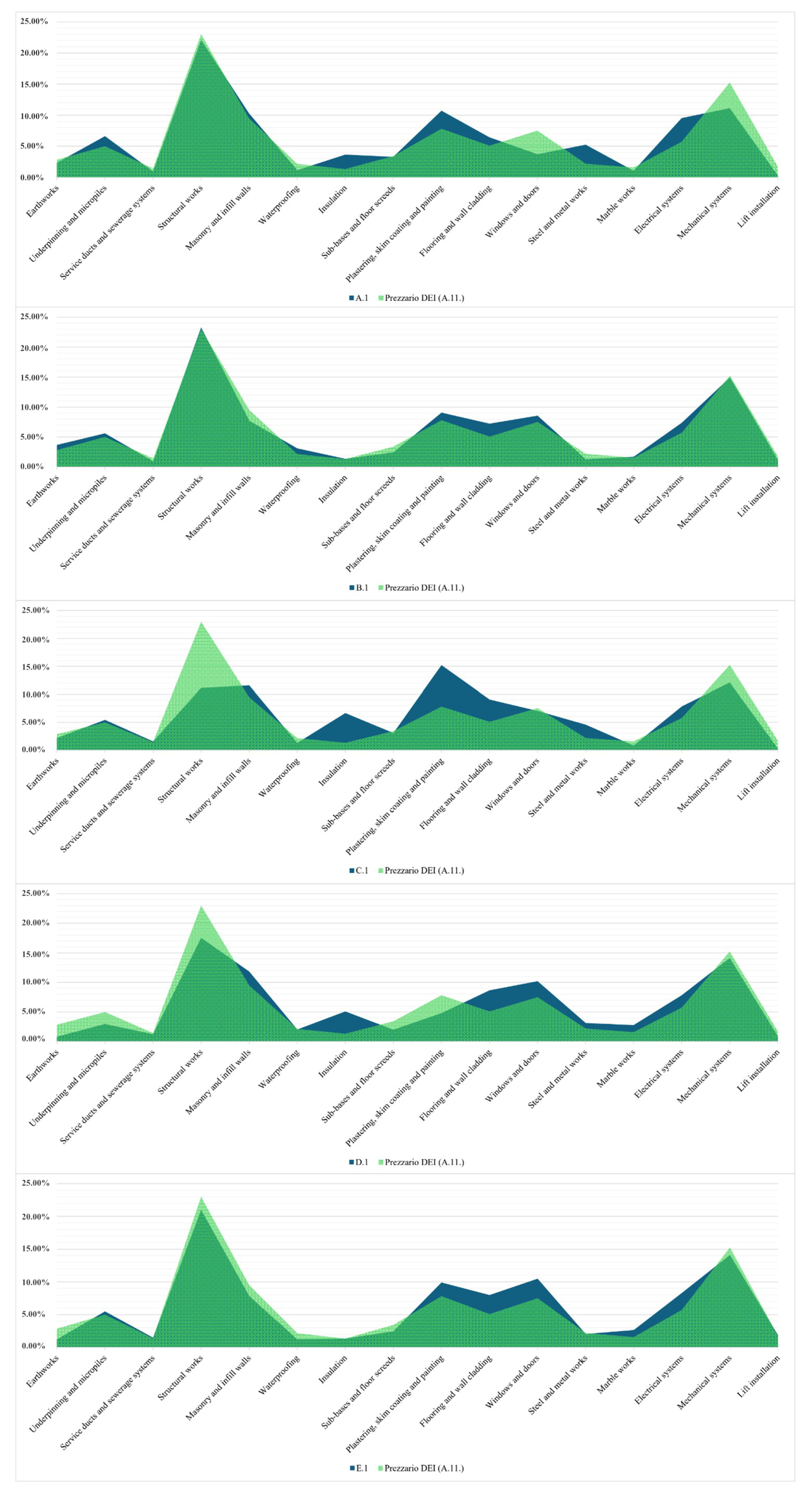
Regarding the comparison between the percentage incidences of intervention categories on the total construction cost between the case studies and typology A.11 of the DEI Prezzario, relevant considerations emerge. For C.1 (RM), percentage deviations exceeding 5% are evidenced in certain cases. Specifically, the percentage values for the categories “plasters, renders and painting” and “insulation” exceed the DEI Prezzario values by 7.40% and 5.33%, respectively. Conversely, for the “structures” category, the DEI Prezzario incidence exceeds the case study value by 11.90%. In light of these discrepancies, it is essential to note that the C.1 case study constitutes an anomalous case requiring attention, as the analysis reveals specificities that—for reasons specific to (and not further verifiable in) the BoQ development—do not allow this project to be identified as a “standard case” or its outputs to be generalised.

Regarding the other buildings, Figure 5 shows that the values obtained in the case studies present minimal deviations from the DEI Prezzario reference: for A.1 (RM), the maximum deviations are for the “electrical system” category (+3.80% above DEI Prezzario) and “mechanical plant” (DEI Prezzario exceeds the case study by 4.10%); for B.1 (RM), the maximum differentials are for “flooring and cladding” (+2.15% above DEI Prezzario) and “masonry/infill” (DEI Prezzario exceeds the case study by 1.78%); for D.1 (VT), the “structures” category diverges from the DEI Prezzario counterpart by 5.47%; for E.1 (NA), the “joinery and windows” category exceeds the DEI Prezzario value by 2.97%.

3.2. Phase II Results

Building upon the outputs of Phase I—and in view of the results yielded by its validation process—Phase II extends the model to a broader and methodologically differentiated dataset. Notably, case study C.1 has been excluded from the Phase II analysis on account of its excessive heterogeneity relative to the remaining sample, as evidenced by the anomalous deviations identified during the Phase I validation exercise.

3.2.1. Methodology Application: Harmonised Intervention Categories

A fundamental difference between Phase I and Phase II concerns the level of disaggregation achievable for the intervention categories. While Phase I allows analytical decomposition into 30 categories based on detailed BoQ data, Phase II data—provided by economic operators as parametric aggregate values—necessitate a higher-level synthesis. The classification is accordingly revised to 16 harmonised categories, defined to maintain the maximum possible consistency with the Phase I taxonomy while accommodating the structural limitations of the Phase II data sources. This harmonisation was achieved through a systematic aggregation of the 30 Phase I categories into 16 broader groupings: for instance, the “Masonry works” category in Phase II subsumes the Phase I categories of infill walls, partition walls and internal dividing elements; similarly, the “Windows and doors” category consolidates the Phase I distinction between internal and external joinery into a single unified entry. It should be emphasised that no Phase I intervention category was discarded: all 30 were retained and appropriately aggregated into the 16 Phase II groupings, thereby preserving the full informational content of the Phase I taxonomy within the consolidated structure. A further motivation underlying this taxonomic consolidation relates to the objective of enhancing cross-case comparability and ensuring the long-term scalability of the model: by adopting a simplified but internally consistent category structure, the framework gains the flexibility required to accommodate progressively larger datasets—including case studies to be incorporated in future research extensions—without compromising the coherence of comparative analyses. The simplification and aggregation of intervention categories thus serve not only an immediate data-compatibility function, but also a long-term methodological purpose, ensuring that the model retains its analytical validity as the database expands over time. Furthermore, the working cluster dimension of the matrix cannot be replicated in Phase II, as the aggregated nature of the available data makes it impossible to classify Phase II case studies at the cluster level. The Phase II matrix therefore operates exclusively along the category axis, with parametric cost data expressed per SCO and per SUL for the residential portion and the underground level separately.

The reconstruction of missing incidence data for categories with zero or incomplete costs in the Phase II dataset is carried out in two aggregation steps. In Step I, the categories undergo a first aggregation according to technological principles and are subsequently populated directly from the operator data where available (

Table 16. Step I: comparison table of absolute costs and percentage incidences per intervention category for the nine Phase II case studies.

	A.2		B.2		C.2		D.2		E.2		F.2		G.2		H.2		I.2
Earthworks	548,954.01	7.47%	22,062.86	0.31%	10,915.00	0.35%	39,312.50	0.95%	390,000.00	7.59%	70,000.00	1.41%	250,000.00	4.83%	88,041.00	1.21%	89,156.55	0.99%
Foundations	-	-	-	-	-	-	-	-	500,000.00	9.73%	120,000.00	2.41%	263,000.00	5.08%	268,209.00	3.69%	383,836.95	4.27%
Retaining walls	-	-	-	-	-	-	-	-	-	-	-	-	-	-	114,000.00	1.57%	106,026.38	1.18%
Reinforced-concrete works, including floor screeds	1,787,988.07	24.32%	1,824,215.25	25.84%	718,125.95	23.29%	1,029,737.48	24.88%	790,000.00	15.37%	870,000.00	17.49%	830,000.00	16.03%	1,952,250.00	26.89%	1,698,919.22	18.91%
Masonry and plasterboard works (infill walls, partitions and internal dividing elements)	2,370,180.77	32.24%	2,178,441.73	30.85%	970,345.63	31.48%	1,266,780.55	30.60%	1,270,000.00	24.71%	1,470,000.00	29.56%	1,416,000.00	27.35%	642,604.00	8.85%	2,528,750.00	28.14%
Waterproofing	-	-	-	-	3461.26	0.11%	-	-	-	-	-	-	-	-	58,859.50	0.81%	-	-
Thermal and acoustic insulation	-	-	-	-	-	-	-	-	-	-	-	-	-	-	82,286.50	1.13%	67,725.00	0.75%
Painting, decorating, plastering and rendering works	124,411.90	1.69%	151,727.56	2.15%	61,692.78	2.00%	82,800.09	2.00%	-	-	-	-	-	-	712,500.00	9.81%	105,250.00	1.17%
Glazing works	107,337.77	1.46%	98,871.00	1.40%	-	-	106,858.54	2.58%	-	-	-	-	-	-	71,250.00	0.98%	-	-
Carpentry and joinery works	34,036.41	0.46%	54,318.00	0.77%	36,318.23	1.18%	-	-	-	-	-	-	-	-	-	-	-	-
Steel, aluminium and sheet-metal works	179,963.81	2.45%	103,207.78	1.46%	61,110.03	1.98%	29,397.77	0.71%	270,000.00	5.25%	220,000.00	4.42%	265,000.00	5.12%	142,500.00	1.96%	458,850.00	5.11%
Stonework (marble thresholds and flooring)	65,846.28	0.90%	82,864.91	1.17%	54,706.96	1.77%	49,416.04	1.19%	57,000.00	1.11%	100,000.00	2.01%	72,000.00	1.39%	178,125.00	2.45%	99,750.00	1.11%
Internal and external windows, doors and frames	484,009.85	6.58%	468,655.64	6.64%	255,880.86	8.30%	417,485.55	10.09%	375,000.00	7.30%	473,000.00	9.51%	379,550.00	7.33%	570,000.00	7.85%	476,579.86	5.30%
Flooring and wall cladding	401,800.77	5.47%	660,561.54	9.36%	131,439.33	4.26%	125,153.85	3.02%	102,000.00	1.98%	195,000.00	3.92%	163,000.00	3.15%	570,000.00	7.85%	201,000.00	2.24%
Sewerage, water-supply, sanitary, heating, air-conditioning and fire-protection systems	723,565.00	9.84%	805,964.63	11.42%	478,064.73	15.51%	648,848.33	15.68%	545,000.00	10.61%	730,000.00	14.68%	848,400.00	16.39%	1,068,750.00	14.72%	1,396,133.97	15.54%
Electrical and photovoltaic systems	389,681.95	5.30%	442,742.84	6.27%	213,361.32	6.92%	169,938.79	4.11%	435,000.00	8.46%	475,000.00	9.55%	440,000.00	8.50%	356,250.00	4.91%	1,157,395.05	12.88%
Lift installation	30,590.00	0.42%	32,700.00	0.46%	15,840.00	0.51%	21,877.51	0.53%	20,000.00	0.39%	40,000.00	0.80%	40,000.00	0.77%	142,500.00	1.96%	77,700.00	0.86%
External works and landscaping	7904.00	0.11%	11,500.00	0.16%	9700.00	0.31%	-	-	65,000.00	1.26%	30,000.00	0.60%	30,000.00	0.58%	106,875.00	1.47%	60,424.64507	0.67%
Plant hire and temporary works	94,352.92	1.28%	122,737.19	1.74%	61,879.99	2.01%	151,729.54	3.67%	320,000.00	6.23%	180,000.00	3.62%	180,000.00	3.48%	136,086.80	1.87%	78,175.35493	0.87%
Total	7,350,623.51	100%	7,060,570.93	100%	3,082,842.07	100%	4,139,336.54	100%	5,139,000.00	100%	4,973,000.00	100%	5,176,950.00	100%	7,261,086.80	100%	8,985,672.98	100%

Note: Red borders identify missing or incomplete operator-provided cost values requiring reconstruction in Step II.

).

In Step II, missing or incomplete values—identified in Table 16 by red highlighting—are reclassified according to the final Phase II taxonomy and supplemented by applying the disaggregated Phase I mean incidences, the latter reported in

Table 17. Step II: supplementation of missing incidence values using Phase I mean percentages for the nine Phase II case studies.

	A.2		B.2		C.2		D.2		E.2		F.2		G.2		H.2		I.2
Earthworks	548,954.01	7.47%	22,062.86	0.31%	10,915.00	0.35%	39,312.50	0.95%	390,000.00	7.59%	70,000.00	1.41%	250,000.00	4.83%	88,041.00	1.21%	89,156.55	0.99%
Retaining walls	19,111.62	0.26%	18,364.53	0.26%	8018.47	0.26%	10,762.28	0.26%	0.00	0.00%	12,760.72	0.26%	13,465.24	0.26%	114,000.00	1.57%	106,026.38	1.18%
Reinforced-concrete works and foundations	1,768,876.45	24.06%	1,805,846.46	25.58%	710,106.71	23.03%	1,018,975.21	24.62%	1,290,000.00	25.10%	977,239.28	19.65%	1,079,533.72	20.85%	2,220,459.00	30.58%	2,082,756.17	23.18%
Masonry works (infill walls, partitions and internal dividing elements)	2,370,180.77	32.24%	2,178,441.73	30.85%	973,806.89	31.59%	1,266,780.55	30.60%	837,291.06	16.29%	1,051,273.40	21.14%	980,101.85	18.93%	783,750.00	10.79%	2,596,475.00	28.90%
Painting, decorating, plastering and rendering works	124,411.90	1.69%	151,727.56	2.15%	61,692.78	2.00%	82,800.09	2.00%	432,708.94	8.42%	418,726.60	8.42%	435,899.19	8.42%	712,500.00	9.81%	105,250.00	1.17%
Glazing works	107,337.77	1.46%	98,871.00	1.40%	0.00	0.00%	106,858.54	2.58%	0.00	0.00%	0.00	0.00%	0.00	0.00%	71,250.00	0.98%	0.00	0.00%
Carpentry and joinery works	34,036.41	0.46%	54,318.00	0.77%	36,318.23	1.18%	0.00	0.00%	0.00	0.00%	0.00	0.00%	0.00	0.00%	0.00	0.00%	0.00	0.00%
Steel, aluminium and sheet-metal works	179,963.81	2.45%	103,207.78	1.46%	61,110.03	1.98%	29,396.98	0.71%	270,000.00	5.25%	220,000.00	4.42%	265,000.00	5.12%	142,500.00	1.96%	458,850.00	5.11%
Stonework	65,846.28	0.90%	82,864.91	1.17%	54,706.96	1.77%	49,416.04	1.19%	57,000.00	1.11%	100,000.00	2.01%	72,000.00	1.39%	178,125.00	2.45%	99,750.00	1.11%
Internal and external windows, doors and frames	484,009.85	6.58%	468,655.64	6.64%	255,880.86	8.30%	417,485.55	10.09%	375,000.00	7.30%	473,000.00	9.51%	379,550.00	7.33%	570,000.00	7.85%	476,579.86	5.30%
Flooring and wall cladding	401,800.77	5.47%	660,561.54	9.36%	131,439.33	4.26%	80,863.79	1.95%	102,000.00	1.98%	195,000.00	3.92%	163,000.00	3.15%	570,000.00	7.85%	201,000.00	2.24%
Sewerage, water-supply, sanitary, heating, air	723,565.00	9.84%	805,964.63	11.42%	478,064.73	15.51%	648,848.33	15.68%	545,000.00	10.61%	730,000.00	14.68%	848,400.00	16.39%	1,068,750.00	14.72%	1,396,133.97	15.54%
Electrical and photovoltaic systems	389,681.95	5.30%	442,742.84	6.27%	213,361.32	6.92%	169,938.79	4.11%	435,000.00	8.46%	475,000.00	9.55%	440,000.00	8.50%	356,250.00	4.91%	1,157,395.05	12.88%
Lift installation	30,590.00	0.42%	32,700.00	0.46%	15,840.00	0.51%	21,877.51	0.53%	20,000.00	0.39%	40,000.00	0.80%	40,000.00	0.77%	142,500.00	1.96%	77,700.00	0.86%
External works and landscaping	7904.00	0.11%	11,500.00	0.16%	9700.00	0.31%	44,290.85	1.07%	65,000.00	1.26%	30,000.00	0.60%	30,000.00	0.58%	106,875.00	1.47%	60,424.64507	0.67%
Plant hire and temporary works	94,352.92	1.28%	122,737.19	1.74%	61,879.99	2.01%	151,729.54	3.67%	320,000.00	6.23%	180,000.00	3.62%	180,000.00	3.48%	136,086.80	1.87%	78,175.35493	0.87%
Total	7,350,623.51 €	100%	7,060,566.67	100%	3,082,841.30	100%	4,139,336.54	100%	5,139,000.00	100%	4,973,000.00	100%	5,176,950.00	100%	7,261,086.80	100%	8,985,672.98	100%

Note: Blue borders identify values reconstructed using the corresponding mean percentage incidences derived from Phase I.

with blue highlighting (Table 17).

Subsequently, all Phase I intervention categories pertaining to the four selected Phase I case studies were re-aligned to the final 16 harmonised categories adopted in Phase II, enabling a fully integrated comparison across the entire sample. In order to assess the proportion between observed and reconstructed data, a sensitivity analysis was carried out, yielding an overall incidence of reconstructed values of approximately 2.50% across the dataset—a level deemed acceptable for the purposes of the present study.

Table 18. Percentage-incidence matrix for the 16 harmonised intervention categories across the 11 integrated case studies (Phase I + Phase II), including the Rome average.

	Phase I		Phase II
	A.1	B.1	A.2	B.2	C.2	D.2	E.2	F.2	G.2	H.2	I.2	Rome Average
Earthworks	2.31%	3.59%	7.47%	0.31%	0.35%	0.95%	7.59%	1.41%	4.83%	1.21%	0.99%	2.82%
Retaining walls	1.03%	0.00%	0.26%	0.26%	0.26%	0.26%	0.00%	0.00%	0.00%	1.57%	1.18%	0.48%
Reinforced-concrete works and foundations	31.48%	32.10%	24.06%	25.58%	23.03%	24.62%	25.10%	19.65%	20.85%	30.58%	23.18%	25.48%
Masonry works (infill walls, partitions and internal dividing elements)	14.86%	10.25%	32.24%	30.85%	31.59%	30.60%	16.29%	21.14%	18.93%	10.79%	28.90%	22.40%
Painting, decorating, plastering and rendering works	10.54%	8.84%	1.69%	2.15%	2.00%	2.00%	8.42%	8.42%	8.42%	9.81%	1.17%	5.77%
Glazing works	0.00%	0.00%	1.46%	1.40%	0.00%	2.58%	0.00%	0.00%	0.00%	0.98%	0.00%	0.58%
Carpentry and joinery works	0.00%	0.25%	0.46%	0.77%	1.18%	0.00%	0.00%	0.00%	0.00%	0.00%	0.00%	0.24%
Steel, aluminium and sheet-metal works	5.15%	1.27%	2.45%	1.46%	1.98%	0.71%	5.25%	4.42%	5.12%	1.96%	5.11%	3.17%
Stonework	1.05%	1.68%	0.90%	1.17%	1.77%	1.19%	1.11%	2.01%	1.39%	2.45%	1.11%	1.44%
Internal and external windows, doors and frames	3.67%	8.35%	6.58%	6.64%	8.30%	10.09%	7.30%	9.51%	7.33%	7.85%	5.30%	7.36%
Flooring and wall cladding	6.33%	7.04%	5.47%	9.36%	4.26%	1.95%	1.98%	3.92%	3.15%	7.85%	2.24%	4.87%
Sewerage, water-supply, sanitary, heating, air conditioning and fire-protection systems	12.77%	15.45%	9.84%	11.42%	15.51%	15.68%	10.61%	14.68%	16.39%	14.72%	15.54%	13.83%
Electrical and photovoltaic systems	9.38%	7.19%	5.30%	6.27%	6.92%	4.11%	8.46%	9.55%	8.50%	4.91%	12.88%	7.59%
Lift installation	0.30%	1.12%	0.42%	0.46%	0.51%	0.53%	0.39%	0.80%	0.77%	1.96%	0.86%	0.74%
External works and landscaping	0.00%	0.16%	0.11%	0.16%	0.31%	1.07%	1.26%	0.60%	0.58%	1.47%	0.67%	0.58%
Plant hire and temporary works	1.63%	2.70%	1.28%	1.74%	2.01%	3.67%	6.23%	3.62%	3.48%	1.87%	0.87%	2.64%

and Figure 6 present the final comparison of percentage incidences across all 11 case studies (2 Phase I + 9 Phase II) for the 16 harmonised categories, together with the average profile for the Rome subsample and the overall total average.

The distribution is consistently polarised, with the structural and building works (reinforced concrete works and foundations; masonry works) and the mechanical/sanitary system (sewerage, water supply, plumbing and heating systems) absorbing the largest shares of the total cost. The average incidence profile for Rome provides the synthetic reference vector for prospective cost estimation.

3.2.2. Validation Against CRESME Benchmarks

Validation of the Phase II results is conducted through comparison with the CRESME benchmark for residential construction costs in the Rome area, accessed via the AWN platform [35]. The comparison is structured at the level of macrocategories: civil/building works, structures, electrical systems, other systems and hires, safety and provisional works. With respect to the Phase I taxonomy—which comprised four macrocategories—the Phase II validation framework introduces a fifth macrocategory, “hires, safety and provisional works”, reflecting both the specific cost structure of the Phase II dataset and the need to align the comparison with the full macrocategory articulation of the CRESME benchmark (

Table 19. Validation of Phase II results: comparison of macrocategory percentage incidences (all 13 case studies and Rome average) against the CRESME benchmark [35]. Absolute deviations are reported for each macrocategory.

Macro Categories	Phase I				Phase II
	E.1	D.1	A.1	B.1	A.2	B.2	C.2	D.2	E.2	F.2	G.2	H.2	I.2	Rome Average	Total Average	Cresme	Abs. Diff.
Building works	43.42%	49.70%	41.61%	37.84%	51.36%	53.96%	51.40%	50.20%	41.62%	50.03%	44.92%	43.15%	44.50%	46.42%	46.44%	54.39%	7.97%
Structures	29.78%	22.01%	34.82%	35.70%	31.79%	26.15%	23.65%	25.83%	32.69%	21.32%	25.94%	33.36%	25.35%	28.78%	28.34%	31.63%	2.85%
Electrical systems	8.21%	7.40%	9.38%	7.19%	5.30%	6.27%	6.92%	4.11%	8.46%	9.55%	8.50%	4.91%	12.88%	7.59%	7.62%	5.19%	2.40%
Other systems	17.33%	15.38%	12.57%	16.57%	10.26%	11.88%	16.02%	16.20%	10.69%	15.48%	17.16%	16.68%	16.40%	14.54%	14.82%	8.79%	5.75%
Site setup, rentals and temporary works	1.27%	5.52%	1.63%	2.70%	1.28%	1.74%	2.01%	3.67%	6.23%	3.62%	3.48%	1.87%	0.87%	2.65%	2.76%

).

The comparison evidences an average absolute deviation of approximately 4.75 percentage points across the five macrocategories, confirming a satisfactory overall coherence between the study results and the sectoral benchmark. The most significant deviations are observed for civil/building works (+7.97 p.p.) and other systems (+5.77 p.p.), while structures (2.85 p.p.) and electrical systems (2.40 p.p.) show more contained differences. The pattern reflects a lower incidence of civil works and a higher incidence of plant systems in the study sample relative to the CRESME reference, consistent with the energy class A+ standard adopted across all Rome-based case studies.

3.2.3. Operative Tools: Project Sheets, GIS Map and OMI Comparison

Phase II produces three categories of operative outputs, each addressing a distinct dimension of the updatable monitoring model: standardised project sheets for project-level cost estimation; a GIS-based territorial cost map for spatial analysis; a comparison with OMI market data for contextualisation of construction costs within the real-estate value framework.

The project sheets produced for Phase II adopt a uniform template (Figure 7), structured around the 16 harmonised categories. For each case study, the sheet reports the total cost and percentage incidence per category, the residential/basement split, and the parametric unit costs per SCO and per SUL. A total of 13 project sheets have been compiled—4 from Phase I and 9 from Phase II—enabling direct cross-phase comparison.

The spatial distribution of updated unit construction costs across the Rome case studies is represented through a GIS-based heat map (Figure 8), developed using QGIS. The map represents a cost density surface calibrated on the SCO-based unit construction costs of the eleven Rome case studies (A.1, B.1 from Phase I; A.2–I.2 from Phase II). The chromatic gradient from light green (lower costs) to red (higher costs) provides a spatially continuous representation of construction cost intensity across the urban territory. While the progressive expansion of the sample remains one of the primary objectives identified for the future development of this work, the interpolation analysis presented here constitutes a foundational reference model from which a first interpretive reading can already be drawn. The GIS tool contributes to the spatial analysis of construction costs by highlighting a clear cost gradient: unit construction costs tend to increase as one approaches Rome’s historic centre, and to decrease progressively towards the peripheral areas. This pattern is attributable primarily to exogenous factors—including the architectural and landscape constraints applicable in more central urban contexts, which typically prescribe the use of higher-quality finishing materials, and the more penalising site accessibility conditions imposed by the morphological characteristics of the Roman urban fabric.

The OMI comparison contextualises Phase II construction cost data within the prevailing real-estate market values in the respective urban zones. Figure 9 compares the 2025-updated construction costs—the update having been carried out by applying the ISTAT index “Indice del costo di costruzione di un fabbricato residenziale” [37] to align each case study’s original cost data to the current reference year—against the corresponding OMI market values [36].

The OMI analysis constitutes a corollary to the primary thesis of the study rather than a central analytical output: it provides a practically useful reference for economic operators seeking to evaluate, for each urban zone or microzone, the differential between construction expenditure and achievable market value—a direct indicator of the potential spending/profit margin of a residential development operation. It should nonetheless be acknowledged that this represents an initial and deliberately simplified comparison: OMI market values incorporate a range of additional cost components—including land acquisition, financing, professional fees, taxes, marketing expenditure and developer risk—that are not captured in the construction cost data presented in this study and that the economic operator will necessarily face. The comparison should therefore be read as a directional instrument rather than a precise measure of project profitability.

3.2.4. Determination of the Average Construction Costs

On the basis of the eleven Rome-based case studies—validated through the iterative homogenisation and CRESME [35] cross-check described above—the average unit construction cost for residential new construction in the Municipality of Rome (updated to 2025) is as follows:

• approximately EUR 2200/m² SUL;
• approximately EUR 1800/m² SCO.

The unit cost range across the eleven cases spans approximately EUR 1187 to 2341/m² SCO, reflecting variability attributable to building quality, construction technology, site conditions and the temporal evolution of input costs between 2017 and 2023.

An objective screening for potentially anomalous observations was performed using the Generalised Extreme Studentized Deviate (ESD) procedure [38], allowing for up to three candidate anomalous observations (

Table 20. Generalised Extreme Studentized Deviate (ESD) test for the identification of potential anomalous observations in SCO-based unit construction costs.

Iteration	Sample Size, n	Mean [EUR/m2]	SD [EUR/m2]	Candidate Extreme Observation	Unit Construction Cost [EUR/m2]	ESD Statistic, Ri	Critical Value, λi
1	11	1750.36	382.92	A.2	2341.32	1.543	2.355
2	10	1691.27	346.75	C.2	1187.58	1.453	2.290
3	9	1747.23	316.28	F.2	1288.33	1.451	2.215

Note: The Generalised ESD procedure was performed at a significance level of α = 0.05, allowing for a maximum of three candidate extreme observations. At each iteration, the observation with the largest absolute standardised deviation from the sample mean was temporarily removed. Since R_i < λ_i at all three iterations, none of the observations can be classified as a statistically significant outlier at the 5% level. A.2, C.2 and F.2 are therefore identified as the three most extreme observations in the dataset and are considered separately in the subsequent descriptive and sensitivity analyses.

).

The sequential analysis identified A.2, C.2 and F.2 as the three most extreme observations in the dataset. However, none exceeded the critical threshold at the 5% significance level (Figure 10).

The remaining eight observations yield a mean SCO-based unit cost of approximately EUR 1805/m², a median of approximately EUR 1853/m² and a coefficient of variation of 15.7%. The resulting reference value of approximately EUR 1800/m² should therefore be interpreted as a descriptive central estimate for the core case-study group rather than as an inferential population estimate.

The convergence between Phase I (EUR 1936/m² SCO for Rome, excluding C.1) and Phase II (EUR 1800/m² SCO)—derived through methodologically independent approaches and substantially different data sources—represents strong evidence of the internal consistency of the integrated model and supports its use as a reliable reference tool for residential construction cost estimation in Rome.

4. Discussions

4.1. Phase I: Methodological Outcomes and Interpretive Findings

The results obtained in Phase I provide a rigorous empirical foundation for the assessment of residential construction costs through a WBS-based decomposition approach. The analysis of five case studies—four located in the Municipality of Rome and one in each of Viterbo and Quarto (NA)—reveals a consistent internal structure in the distribution of costs across working clusters and intervention categories, notwithstanding the inherent variability associated with project-specific design choices.

With respect to the homogenisation coefficients (IC) assigned to working clusters, a marked degree of dispersion emerges across the case studies (Figure 11).

In particular, the “lift shafts” cluster exhibits the most pronounced variability, with incidence values on the unit construction cost of the main surface exceeding 100% in the D.1 (VT) and B.1 (RM) projects. This result reflects deliberate design decisions entailing elevated vertical-circulation investments, which translate directly into disproportionate cost contributions from this cluster. Conversely, in the A.1 (RM) and C.1 (RM) case studies, the corresponding coefficients are substantially lower, at 15.87% and 22.74%, respectively, indicating a more contained impact of lift infrastructure on the overall construction cost. Analogous variability is observed for the “loggias, balconies and terraces”, “external arrangements” and “semi-basement level” clusters, underscoring the sensitivity of unit costs to project-specific typological and technological configurations.

Notwithstanding this unit-level variability, the analysis of the total cost incidences of working clusters relative to the aggregate construction cost of each intervention reveals a substantially more uniform distribution (Figure 12).

This compensatory mechanism—whereby project-level design specificities that generate elevated unit costs in certain clusters are offset by complementary reductions in others—confirms the structural stability of the cost model at the aggregate level. This finding is of particular relevance for parametric analysis, as it validates the use of total incidence profiles as robust reference benchmarks applicable across projects with differing design characteristics.

The analysis of percentage incidences by intervention category corroborates these observations (Figure 13).

With the notable exceptions of C.1 (RM) and, to a lesser extent, D.1 (VT) case studies, the distribution of costs across intervention categories follows a broadly consistent pattern across all five projects. The divergences observed in the C.1 case study—including a deviation exceeding 11.90% for the “structures” category and values of 7.40% and 5.33% for “plasters, renders and painting” and “insulation” respectively, when compared against the DEI Prezzario benchmark—confirm the anomalous character of this case study and justify its exclusion from the derivation of aggregate reference parameters.

For the remaining four case studies, deviations from the DEI Prezzario benchmark are contained within acceptable ranges (generally below 5%), lending external validity to the applied methodology. Among the most economically significant intervention categories identified in the Phase I Rome sample are “reinforced concrete and laterocement structures” (22.34%), “hydro-sanitary and thermal plant” (13.03%) and “electrical system” (7.56%). These three categories collectively account for a substantial share of the total construction cost, confirming the central role of structural and plant components in the economic dynamics of new residential construction.

The comparison between the two parametric denominators—SUL and SCO—yields a finding of significant methodological interest. For the Rome case studies (excluding C.1), unit construction costs expressed per SUL range from a minimum of EUR 2480/m² to a maximum of EUR 2790/m², with a mean of EUR 2635/m², a value closely aligned with the DEI Prezzario benchmark of approximately EUR 2600/m² for analogous building typologies. When the same costs are expressed per SCO, the values are systematically lower: the range narrows to EUR 1795–2080/m², with a mean of EUR 1937.50/m². The resulting mean differential of approximately −26% between the SUL-based and SCO-based unit costs is a direct consequence of the homogenisation procedure applied to accessory, underground, common and technical surfaces, which redistributes the construction cost over a broader, conventionally equivalent built area. This differential constitutes a structural feature of the model rather than a measurement artefact and underlines the importance of adopting a clearly defined parametric denominator when comparing construction cost data across different projects or contexts. Extending the analysis to provincial contexts, lower unit costs are recorded: EUR 2205/m² SUL and EUR 1445/m² SCO for D.1 (VT), and EUR 1800/m² SUL and EUR 1270/m² SCO for E.1 (NA). Considering all four case studies (excluding C.1), the overall means are EUR 2320/m² SUL and EUR 1650/m² SCO, reflecting the structural differences in labour markets, supply chains and logistical conditions across territorial contexts.

In order to enhance the procedural transparency and international replicability of the proposed methodology,

Table 21. Comparative overview of official or institutionally recognised construction cost references by country.

Country	Reference
UK	BCIS CapX; Spon’s Architects’ and Builders’ Price Book
Germany	BKI Baukosten Gebäude Neubau 2026
French	Batiprix; INSEE—indices construction
Spain	CYPE Generador de Precios; ITeC BEDEC; basi regionali pubbliche come BCCA
Netherlands	Andalucía; BDB Bouw (kosten)data; BouwkostenKompas
USA	RSMeans Data Online
Australia	Rawlinsons Australian Construction Handbook 2026 e Construction Cost Guide 2026
Canada	Altus Group—2026 Canadian Cost Guide
Brasil	CUB/m2—CBIC/SindusCon statali; SINAPI—CAIXA

reports a selection of official or institutionally recognised construction cost references available in comparable national contexts, providing practitioners and researchers operating outside Italy with equivalent benchmarking instruments.

4.1.1. Corrective Factors

The reference unit costs derived from the Phase I analysis apply to new construction interventions in urban transformation and expansion areas under standard site accessibility conditions. Where project-specific circumstances deviate from these conditions, appropriate corrective factors must be applied. Two principal categories are identified: site accessibility and demolition.

Site Accessibility

Urban fabrics exhibit an accessibility gradient that progresses from the historic centre—characterised by greater logistical complexity, restricted site configurations and higher operational costs—towards peripheral and transformation areas, where standard site organisation conditions apply. Drawing on CRESME data for different site accessibility scenarios, percentage corrective factors have been derived for each location typology (

Table 22. Percentage corrective factor for site accessibility.

Site Accessibility	Percentage Increase
From normal to restricted	8.00%
From restricted to severely restricted	12.96%
From normal to severely restricted	22.00%

). The case studies analysed are predominantly situated in urban transformation and expansion areas, classified as presenting standard accessibility conditions, and accordingly do not require the application of a positive corrective factor.

Demolition

The Phase I dataset includes both new construction and demolition-and-reconstruction interventions. In deriving the reference unit construction costs, only cost items directly attributable to new construction were retained; demolition costs were treated separately and quantified through dedicated corrective factors. The percentage incidence of the demolition item on the total construction cost was determined for case studies B.1 (RM) and D.1 (VT), yielding a mean value of 1.85%. Comparison with the corresponding DEI Prezzario values for typologies A.9, A.10 and A.11—which report a mean incidence of 1.50% confirms the close alignment between the empirical and benchmark estimates. A corrective factor of 2.00% was adopted for precautionary purposes (

Table 23. Percentage incidence of the demolition item.

	Demolition Cost	Total Construction Cost	Percentage Incidence	Average	Correction Factor
Case studies
B.1	EUR 482,151.90	EUR 19,151,210.57	2.52%	1.85%	2.00%
D.1	EUR 64,278	EUR 5,417,250.71	1.19%
DEI Prezzario
A.9.	EUR 16,782	EUR 3,022,548	0.56%	1.50%
A.10.	EUR 429,898	EUR 11,799,706	3.64%
A.11.	EUR 15,852	EUR 5,468,541	0.29%

).

In this context, the applicable framework for construction and demolition waste should be distinguished by function. D.M. 28 June 2024, No. 127 [39] establishes the end-of-waste criteria for inert construction and demolition waste. For public building procurement subject to the Italian Minimum Environmental Criteria, the 2022 CAM Edilizia [40] requires that at least 70% by weight of non-hazardous construction and demolition waste generated on site be prepared for reuse, recycling or other material recovery. UNI/PdR 75:2020 [41] provides an operational methodology for selective deconstruction and the recovery of construction and demolition waste. These requirements may introduce additional cost components in demolition-and-reconstruction projects and should therefore be considered explicitly in project cost assessments (Table 23).

4.2. Phase II: Extension, Harmonisation and Validation

Phase II extends the integrated monitoring model to a substantially larger and methodologically more heterogeneous dataset. The nine additional case studies, all located within the Municipality of Rome and sourced directly from cost statements provided by the economic operators involved in their construction, required a significant reworking of the analytical framework—both in terms of the taxonomic structure of intervention categories and in terms of the data reconstruction procedure for incomplete cost profiles.

The reduction from 30 analytical categories (Phase I) to 16 harmonised categories (Phase II) was driven by two complementary considerations. First, the parametric and aggregated nature of the operator-supplied data precluded the level of analytical disaggregation achievable on the basis of BoQ in Phase I. Second, and of equal methodological significance, the consolidation of the taxonomic structure was motivated by the objective of enhancing cross-case comparability and ensuring the long-term scalability of the model. By adopting a simplified but internally consistent category structure, the framework gains the flexibility required to accommodate progressively larger datasets—including case studies to be incorporated in future research extensions—without compromising the coherence of comparative analyses. The 16 harmonised categories thus represent not merely an adaptation to data-source constraints, but a deliberate design choice oriented towards the construction of a durable and extensible cost-monitoring system.

The two-step data reconstruction procedure—whereby missing incidence values in the Phase II dataset were supplemented by applying Phase I mean incidences, reclassified according to the Phase II taxonomy—ensures the internal consistency of the resulting cost profiles. This iterative refinement approach, while introducing a degree of indirect inference for incomplete data fields, is methodologically justified by the strong cross-study coherence demonstrated in Phase I and by the conservative nature of the mean-based imputation strategy. The resulting 13-case integrated matrix provides a comprehensive reference framework for the parametric assessment of residential construction costs in the Municipality of Rome.

Validation of the Phase II results through comparison with the CRESME benchmark confirms the overall reliability of the model. The average absolute deviation of approximately 4.75 percentage points across the five macrocategory aggregates reflects a satisfactory level of alignment with the sectoral reference. The most significant deviations—concentrated in the civil/building works (+7.97 p.p.) and other systems (+5.77 p.p.) macrocategories—are consistently interpretable in light of the structural characteristics of the Phase II sample: all eleven Rome-based case studies achieve energy class A+, entailing a systematically higher incidence of plant-engineering components relative to the broader market benchmark represented by CRESME. This systematic offset is therefore not a methodological artefact but a substantive reflection of the sample’s technological profile.

The convergence between the Phase I mean unit cost for Rome (EUR 1936/m² SCO, excluding C.1) and the Phase II estimate (EUR 1800/m² SCO)—derived through methodologically independent approaches from substantially different data sources—constitutes the most robust validation outcome of the integrated model. The modest differential of approximately 7% between the two estimates falls well within the expected range of parametric cost variability and is attributable in part to the temporal evolution of input prices across the 2017–2023 construction period spanned by the Phase II sample. This convergence supports the conclusion that the proposed framework reliably identifies the structural parameters of residential construction costs in the Roman urban context, independently of the specific data source or analytical procedure employed.

4.3. Operational Tools: Interpretive and Monitoring Functions

Beyond the quantitative results, a central contribution of the present study consists in the development of three categories of operational tools—project sheets, a GIS-based territorial cost map, and an OMI market value comparison framework—each addressing a distinct but complementary dimension of the updatable monitoring system.

The standardised project sheets constitute a flexible decision-support instrument for economic operators, designers, developers and public administrations. Organised around the 16 harmonised categories, each sheet reports total costs and percentage incidences, the residential/underground split, and parametric unit costs per SCO and per SUL. The tool enables the identification of the intervention categories with the greatest economic impact, supports comparison against reference benchmarks, and accommodates project-specific configurations—including cases where underground levels are absent, or certain plant components are supplied separately. At the procurement stage, macrocategory weight profiles provide a concrete reference for contract management and the optimisation of subcontracting arrangements.

The GIS-based heat map renders the spatial distribution of updated unit construction costs across the eleven Rome case studies as a chromatic gradient, from lower values in peripheral areas to higher values in the central urban fabric. This spatial gradient reflects differences in site accessibility, logistical complexity and regulatory constraints across urban zones. Crucially, the map is designed as an updatable instrument: as additional case studies are incorporated, the cost density surface can be progressively updated, enhancing its spatial resolution and statistical reliability. This positions the GIS component as a strategic asset for urban planners, housing policy administrators and real-estate professionals.

The OMI market value comparison contextualises construction costs within the prevailing real-estate value framework of each urban zone. By situating the technical construction cost against market prices, it enables operators to evaluate the economic margin between production cost and transfer value and assess project viability under different market conditions. Cases where construction cost approaches or exceeds the OMI market value signal conditions of constrained feasibility or regulated-housing pressure; wider margins indicate more favourable conditions for private construction initiatives.

4.4. Positioning Within the Existing Literature

The methodological approach developed in the present study aligns with several established lines of inquiry in construction economics. The emphasis on a transparent, pro-cess-oriented cost-calculation framework—as opposed to black-box predictive model-ling—resonates with Oberlender and Trost (2001) [4], Akintoye (2000) [5], and the quanti-ty-surveying and cost-planning tradition represented by Ferry et al. (1999) [6], Kirkham et al. (2015) [7], Seeley (1996) [8] and Ashworth and Perera (2015) [9]. These sources emphasise that estimate reliability depends on the quality and coherence of the underlying calculation process, including project decomposition, cost attribution and progressively detailed measurement. The WBS-based framework proposed in this study operationalises this principle by making the cost-calculation procedure traceable, verifiable and replicable.

The introduction of the SCO as the parametric denominator for the expression of unit construction costs addresses a methodological gap widely acknowledged in the literature on cost benchmarking. By systematically accounting for the incidence of accessory, underground, common and technical spaces through homogenisation coefficients, the SCO parameter provides a more representative and replicable denominator than conventional measures such as SUL or net usable area, whose definitions vary across regulatory contexts and professional conventions. The mean differential of approximately −26% between SUL-based and SCO-based unit costs identified in this study constitutes a quantitatively significant finding that should inform both professional practice and the design of future cost-benchmarking systems.

The spatial dimension introduced through the GIS-based heat map extends the scope of the proposed framework beyond individual project assessment towards territorial cost monitoring, positioning the study within a growing body of work on the spatialisation of construction economics. The integration of GIS tools with parametric cost data enables the identification of spatial cost gradients, the localised calibration of reference benchmarks and the updating of territorial cost pictures as new data become available—functionalities that are of increasing relevance in the context of urban transformation and housing policy design.

5. Conclusions

The present study has proposed, tested and validated a methodological framework for the structured assessment, decomposition and updatable monitoring of residential construction costs. The developed methodological approach is grounded in the Work Breakdown Structure principle and is applied to a set of thirteen case studies located principally within the Municipality of Rome, with additional projects in Viterbo and Quarto (NA). Three principal dimensions structure the findings and contributions of the study.

From a methodological perspective, the WBS-based cost decomposition framework demonstrates its capacity to generate transparent, traceable and replicable construction cost data across heterogeneous project types and data sources. The two-phase research structure—combining analytical BoQ-based decomposition (Phase I) with operator-supplied parametric data (Phase II)—enables the model to accommodate different levels of data granularity without compromising internal consistency or cross-case comparability. The iterative harmonisation procedure, through which Phase I analytical categories are re-aligned to the 16 categories adopted in Phase II, provides a practical and scalable solution to the challenge of integrating cost data from methodologically disparate sources.

From a quantitative perspective, the study establishes a robust reference benchmark for the unit construction cost of new residential buildings in the Municipality of Rome. On the basis of eleven Rome-based case studies, validated through DEI Prezzario and CRESME cross-checks, the average unit cost is estimated at approximately EUR 1800/m² SCO and EUR 2200/m² SUL, updated to 2025. It is important to note that this cost figure encompasses the sole technical construction cost—comprising materials, labour, plant hire and transport—together with the indirect cost components (general overheads and contractor profit), ordinarily amounting to approximately 26.5% of the technical cost. Excluded from this estimate are the costs of land acquisition, professional fees, urbanisation charges and connection fees. For the case studies analysed, reference is made to pre-construction cost estimates; costs pertaining to temporary works (scaffolding) and safety charges are similarly excluded.

From an operational perspective, the three categories of tools produced by the study—project sheets, GIS heat map and OMI comparison framework—translate the analytical outputs of the model into practical decision-support instruments for a wide range of stakeholders.

The results of this study should be read transversally, as components of an integrated methodological system rather than as standalone outputs. Each instrument gains interpretive depth when read in conjunction with the others: the project sheet acquires meaning in relation to the territorial cost picture provided by the GIS map, which in turn is contextualised by the OMI market comparison. This systemic reading is a defining feature of the updatable monitoring model proposed here. To illustrate the operational logic of this integration: an economic operator planning a new residential development in the current year might begin by consulting the open-access GIS cost map to obtain a spatially differentiated picture of unit construction costs across the urban territory of Rome, identifying the zones most compatible with the target cost envelope. The operator could then cross-reference this information with the OMI market values to gauge the achievable sale prices or rental yields in each zone or microzone, thereby assessing the potential economic margin of the operation under different locational scenarios. Finally, drawing on the standardised project sheets, the operator could carry out a personalised cost simulation—entering estimated expenditure for individual intervention categories and obtaining a customised unit construction cost that can be directly compared against both the territorial cost picture and prevailing market values. This integrated sequential workflow is precisely what is meant when the updatable monitoring model is described as a decision-support instrument for economic operators in determining where to build and what morphological and technological quality standard to target.

Several limitations of the present study should be acknowledged. The case study sample, while internally validated, remains confined to a specific urban and regional context and may not be directly generalisable to other Italian regions or European markets. A further consideration pertains to the temporal dimension of the dataset: the case studies analysed were not all built in the current year but span a multi-year construction period extending from 2009 to 2024. As a consequence, the construction costs associated with individual case studies reflect the input-price conditions prevailing at the time of execution and must be systematically updated to the current reference year before being employed as benchmarks. The updatable monitoring framework explicitly accounts for this requirement through its annual cost-updating procedure; nonetheless, users of the derived reference values should remain aware that the degree of temporal proximity between a case study’s construction period and the present directly affects the representativeness of the associated cost benchmark.

These limitations point directly to the principal directions for future research. The most immediate priority consists in expanding the case study database, both in terms of the number of projects and in terms of territorial coverage. A larger sample—encompassing a broader range of urban contexts, construction typologies and quality classes—would enhance the statistical reliability of the reference benchmarks and enable the derivation of differentiated cost profiles for specific sub-markets or territorial zones. The integration of additional case studies into the existing database, facilitated by the scalable taxonomic structure adopted in Phase II, represents the natural next step in the progressive development of the monitoring system.

A second direction concerns the progressive enrichment of the individual operational tools. Each of the three operational tools possesses inherent development potential that may be realised both independently and in integration with the others. Future developments could include the digitalisation and interactive enhancement of the project sheets through web-based or BIM-integrated platforms, the progressive densification of the GIS cost surface through the incorporation of additional georeferenced case studies, and the extension of the OMI comparison framework to encompass rental market values and transformation cost benchmarks. In this perspective, the monitoring system proposed in the present study should be understood not as a completed product but as a scalable infrastructure, whose analytical and operational value grows as new case studies, territorial contexts and methodological refinements are progressively incorporated. Finally, future research should investigate the potential for extending the WBS-based cost decomposition framework to residential renovation and energy-retrofit interventions, which represent a growing share of the construction market in the Italian and European context. The integration of sustainability cost components—including the costs associated with selective demolition, circular economy compliance and the achievement of near-zero energy performance standards—into the monitoring framework would significantly enhance its applicability and policy relevance in the context of the European Green Deal and the EU Renovation Wave initiative.

References

1. Eurostat. Short-Term Business Statistics. Available online: https://ec.europa.eu/eurostat/web/short-term-business-statistics (accessed on 28 July 2026).
2. Regione Lazio. Deliberazione Della Giunta Regionale 14 Aprile 2023, n. 101: Approvazione Della Tariffa dei Prezzi per le Opere Pubbliche Edili ed Impiantistiche del Lazio—Edizione 2023. Available online: https://www.regione.lazio.it/documenti/80338 (accessed on 28 July 2026).
3. Project Management Institute. Practice Standard for Work Breakdown Structures, 3rd ed.; Project Management Institute: Newtown Square, PA, USA, 2019. [Google Scholar]
4. Oberlender, G.D.; Trost, S.M. Predicting accuracy of early cost estimates based on estimate quality. J. Constr. Eng. Manag. 2001, 127, 173–182. [Google Scholar] [CrossRef] [Scilit]
5. Akintoye, A. Analysis of factors influencing project cost estimating practice. Constr. Manag. Econ. 2000, 18, 77–89. [Google Scholar] [CrossRef] [Scilit]
6. Ferry, D.J.; Brandon, P.S.; Ferry, J.D. Cost Planning of Buildings, 7th ed.; Blackwell Science: Oxford, UK, 1999. [Google Scholar]
7. Kirkham, R.; Bataw, A.; Waterman, A.; Greenhalgh, B. Ferry and Brandon’s Cost Planning of Buildings, 9th ed.; John Wiley & Sons: Chichester, UK, 2015. [Google Scholar]
8. Seeley, I.H. Building Economics, 4th ed.; Macmillan: London, UK, 1996. [Google Scholar]
9. Ashworth, A.; Perera, S. Cost Studies of Buildings, 6th ed.; Routledge: London, UK, 2015. [Google Scholar]
10. Soutos, M.; Lowe, D.J. Elemental cost estimating: Current UK practice and procedure. J. Financ. Manag. Prop. Constr. 2011, 16, 147–162. [Google Scholar] [CrossRef] [Scilit]
11. Potts, K. Construction Cost Management: Learning from Case Studies; Taylor & Francis: London, UK, 2008. [Google Scholar]
12. Cerezo-Narváez, A.; Pastor-Fernández, A.; Otero-Mateo, M.; Ballesteros-Pérez, P. Integration of Cost and Work Breakdown Structures in the Management of Construction Projects. Appl. Sci. 2020, 10, 1386. [Google Scholar] [CrossRef] [Scilit]
13. Dopazo, D.A.; Mahdjoubi, L.; Gething, B.; Mahamadu, A.M. An automated machine learning approach for classifying infrastructure cost data. Comput.-Aided Civ. Infrastruct. Eng. 2024, 39, 1061–1076. [Google Scholar] [CrossRef] [Scilit]
14. Vázquez-López, E.; Solís-Guzmán, J.; Marrero, M. A Work Breakdown Structure for Estimating Building Life Cycle Cost Aligned with Sustainable Assessment—Application to Functional Costs. Buildings 2024, 14, 1119. [Google Scholar] [CrossRef] [Scilit]
15. Kim, G.H.; An, S.H.; Kang, K.I. Comparison of construction cost estimating models based on regression analysis, neural networks, and case-based reasoning. Build. Environ. 2004, 39, 1235–1242. [Google Scholar] [CrossRef] [Scilit]
16. Sönmez, R. Conceptual cost estimation of building projects with regression analysis and neural networks. Can. J. Civ. Eng. 2004, 31, 677–683. [Google Scholar] [CrossRef] [Scilit]
17. Lowe, D.J.; Emsley, M.W.; Harding, A. Predicting construction cost using multiple regression techniques. J. Constr. Eng. Manag. 2006, 132, 750–758. [Google Scholar] [CrossRef] [Scilit]
18. Günaydın, H.M.; Doğan, S.Z. A neural network approach for early cost estimation of structural systems of buildings. Int. J. Proj. Manag. 2004, 22, 595–602. [Google Scholar] [CrossRef] [Scilit]
19. Cheng, M.Y.; Tsai, H.C.; Hsieh, W.S. Web-based conceptual cost estimates for construction projects using evolutionary fuzzy neural inference model. Autom. Constr. 2009, 18, 164–172. [Google Scholar] [CrossRef] [Scilit]
20. Rafiei, M.H.; Adeli, H. Novel machine-learning model for estimating construction costs considering economic variables and indexes. J. Constr. Eng. Manag. 2018, 144, 04018106. [Google Scholar] [CrossRef] [Scilit]
21. Stoy, C.; Pollalis, S.; Schalcher, H.R. Drivers for cost estimating in early design: Case study of residential construction. J. Constr. Eng. Manag. 2008, 134, 32–39. [Google Scholar] [CrossRef] [Scilit]
22. Trabucco, D.; Miranda, V. Creating Industry-Accepted Criteria for Measuring Tall Building Floor Area. CTBUH J. 2019, 2019, 34–39. [Google Scholar]
23. Kara, A.; Çağdaş, V.; Işıkdağ, Ü.; Turan, B.O. Towards harmonizing property measurement standards. J. Spat. Inf. Sci. 2018, 17, 87–119. [Google Scholar] [CrossRef] [Scilit]
24. Ma, M.; Zhang, S.; Liu, J.; Yan, R.; Cai, W.; Zhou, N.; Yan, J. Building Floorspace and Stock Measurement: A Review of Global Efforts, Knowledge Gaps, and Research Priorities. Nexus 2025, 2, 100075. [Google Scholar] [CrossRef] [Scilit]
25. Flyvbjerg, B.; Holm, M.K.S.; Buhl, S.L. Underestimating costs in public works projects: Error or lie? J. Am. Plan. Assoc. 2002, 68, 279–295. [Google Scholar] [CrossRef] [Scilit]
26. Flyvbjerg, B.; Holm, M.K.S.; Buhl, S.L. What causes cost overrun in transport infrastructure projects? Transp. Rev. 2004, 24, 3–18. [Google Scholar] [CrossRef] [Scilit]
27. Cantarelli, C.C.; Flyvbjerg, B.; Molin, E.J.E.; van Wee, B. Cost overruns in large-scale transportation infrastructure projects: Explanations and their theoretical embeddedness. Eur. J. Transp. Infrastruct. Res. 2010, 10, 5–18. [Google Scholar] [CrossRef] [Scilit]
28. Ahiaga-Dagbui, D.D.; Smith, S.D. Dealing with construction cost overruns using data mining. Constr. Manag. Econ. 2014, 32, 682–694. [Google Scholar] [CrossRef] [Scilit]
29. Olawale, Y.A.; Sun, M. Cost and time control of construction projects: Inhibiting factors and mitigating measures in practice. Constr. Manag. Econ. 2010, 28, 509–526. [Google Scholar] [CrossRef] [Scilit]
30. ElSawy, I.; Hosny, H.; Abdel Razek, M. A neural network model for construction projects site overhead cost estimating in Egypt. Int. J. Comput. Sci. Issues 2011, 8, 273–283. [Google Scholar]
31. Elmousalami, H.H. Comparison of artificial intelligence techniques for project conceptual cost prediction: A case study and comparative analysis. IEEE Trans. Eng. Manag. 2021, 68, 183–196. [Google Scholar] [CrossRef] [Scilit]
32. Budayan, C.; Dikmen, I.; Birgonul, M.T. Construction cost map of European countries. Eng. Econ. 2020, 65, 135–157. [Google Scholar] [CrossRef] [Scilit]
33. Zhang, S.; Migliaccio, G.C.; Zandbergen, P.A.; Guindani, M. Empirical assessment of geographically based surface interpolation methods for adjusting construction cost estimates by project location. J. Constr. Eng. Manag. 2014, 140, 04014015. [Google Scholar] [CrossRef] [Scilit]
34. Collegio degli Ingegneri e Architetti di Milano. Prezzi Tipologie Edilizie 2024; DEI Tipografia del Genio Civile: Rome, Italy, 2024; Available online: https://www.build.it/prezzari/tipologici/tipologie-edilizie/prezzi-tipologie-edilizie-2024/ (accessed on 10 July 2026).
35. Consiglio Nazionale degli Architetti, Pianificatori, Paesaggisti e Conservatori; CRESME. Costi Costruzione Edilizia. Available online: https://costi-costruzione.cresme.it/default.aspx (accessed on 28 July 2026).
36. Agenzia delle Entrate. Banca Dati Delle Quotazioni Immobiliari—Osservatorio del Mercato Immobiliare. Available online: https://www1.agenziaentrate.gov.it/servizi/geopoi_omi/index.htm (accessed on 28 July 2026).
37. ISTAT. Indice del Costo di Costruzione di un Fabbricato Residenziale; Istituto Nazionale di Statistica: Rome, Italy, 2020; Available online: https://www.istat.it (accessed on 1 September 2026).
38. Rosner, B. Percentage Points for a Generalized ESD Many-Outlier Procedure. Technometrics 1983, 25, 165–172. [Google Scholar] [CrossRef]
39. Ministero dell’Ambiente e della Sicurezza Energetica. Decreto 28 Giugno 2024, n. 127: Regolamento Recante Disciplina Della Cessazione Della Qualifica di Rifiuto dei Rifiuti Inerti da Costruzione e Demolizione, Altri Rifiuti Inerti di Origine Minerale, ai Sensi Dell’articolo 184-Ter, Comma 2, del Decreto Legislativo 3 Aprile 2006, n. 152. Gazzetta Ufficiale, Serie Generale 2024, No. 213. 11 September 2024. Available online: https://www.gazzettaufficiale.it/eli/id/2024/09/11/24G00144/sg (accessed on 28 July 2026).
40. Ministero della Transizione Ecologica. Decreto 23 Giugno 2022, n. 256: Criteri Ambientali Minimi per L’affidamento del Servizio di Progettazione di Interventi Edilizi, per L’affidamento dei Lavori per Interventi Edilizi e per L’affidamento Congiunto di Progettazione e Lavori per Interventi Edilizi. Gazzetta Ufficiale, Serie Generale 2022, No. 183. 6 August 2022. Available online: https://www.gazzettaufficiale.it/eli/id/2022/08/06/22A04307/sg (accessed on 28 July 2026).
41. UNI/PdR 75:2020; Decostruzione Selettiva—Linea Guida per la Decostruzione Selettiva e il Recupero dei Rifiuti in Un’ottica di Economia Circolare. UNI: Milan, Italy, 2020. Available online: https://www.uni.com/decostruzione-selettiva-pubblicata-la-uni-pdr-75-2020/ (accessed on 5 July 2026).
Figure 1. Methodological flowchart. Blue boxes indicate methodological steps; green boxes indicate validation steps against sectoral benchmarks.
Buildings 16 03732 g001
Figure 2. Geographic distribution of the eleven Rome-based case studies.
Buildings 16 03732 g002
Figure 3. Analytical scheme of the matrix model.
Buildings 16 03732 g003
Figure 4. Extract from the project sheet by intervention categories.
Buildings 16 03732 g004
Figure 5. Comparison of percentage incidences by intervention category between each case study and the DEI Prezzario (typology A.11).
Buildings 16 03732 g005
Figure 6. Final application: percentage incidence table and comparison line chart for 16 harmonised intervention categories across all 11 case studies (Phase I + Phase II), with Rome average highlighted.
Buildings 16 03732 g006
Figure 7. Phase II project sheet template: standardised layout with 16 harmonised intervention categories and interactive navigation; below, comparison of Phase I and Phase II category taxonomies.
Buildings 16 03732 g007
Figure 8. GIS heat map of unit construction costs per SCO (updated to 2025) for the eleven Rome-based case studies. Source: QGIS elaboration by the research team.
Buildings 16 03732 g008
Figure 9. Comparison of 2025-updated construction costs vs. OMI market values per case study.
Buildings 16 03732 g009
Figure 10. Phase II results: SCO unit construction costs per case study ordered by construction quality class (low/medium/high). The vertical dashed lines indicate the lower and upper bounds of the cost range; the green shaded area highlights the cluster of observations retained for the core statistical analysis.
Buildings 16 03732 g010
Figure 11. Comparison of the homogenisation coefficients (IC) of working clusters across the case studies.
Buildings 16 03732 g011
Figure 12. Comparison of working cluster weights relative to the total construction cost for each case study.
Buildings 16 03732 g012
Figure 13. Comparison of percentage incidences by intervention category for each case study.
Buildings 16 03732 g013