The Impact of Controlled-Chamber U-Value Measurements on Building Energy Modelling: Evidence from Sustainable Wall Materials

Abstract

Building energy models rely on the wall thermal transmittance (U-value), yet, for locally available and novel sustainable materials, this input is usually taken from tabulated conductivities rather than measured, introducing an unquantified bias. The conductivity (k) and transmittance (U) of five locally available sustainable wall materials for social housing in the Mexico City Metropolitan Area—an adobe-type block, volcanic stone, tepetate ashlar, and solid and hollow sargassum-based concrete (SBC)—were estimated from heat-flux and temperature measurements on $1{\mathrm{m}}^2$ specimens tested in a controlled two-room chamber (17 and 30 °C) using the ISO 9869-1 heat-flow-meter method, and benchmarked against a conventional concrete reference held at its tabulated value. Three reductions were compared—the ISO 9869-1 average method, a direct air-to-air estimate, and a dynamic grey-box (2R1C) model—which agreed within about 5%, with 1–6% repeatability. For four materials, the estimated U was 15–32% below the tabulated value, whereas the hollow SBC block exceeded it ($+11\%$), showing that tabulated inputs can err in either direction. Propagated through a whole-building EnergyPlus model of a representative social-housing archetype, the measurement-derived transmittances changed the predicted annual heating-plus-cooling demand by $-28$ to $-42\%$ for the four better-insulating walls and $+19\%$ for the hollow block—a shift large enough to reorder the materials—scaling almost linearly with U ($R^2=0.95$). The values are reported as controlled-chamber, element-level estimates, and an open, simulation-ready material database accompanies the paper.

1. Introduction

Buildings account for a large share of global energy use and carbon emissions [1,2], and the drive to decarbonise housing has intensified the search for sustainable, locally sourced alternatives for the building envelope—earthen blocks, quarried minerals, industrial by-products and, increasingly, bio-based and waste-derived composites—whose low-processing supply chains reduce embodied carbon [3]. Their operational benefit, however, depends on the envelope’s thermal transmittance (U), and for these materials U is usually taken from a tabulated conductivity rather than measured. In the temperate, heating-relevant climate of the Mexico City Metropolitan Area (ZMVM), where the wall governs operational energy over the building life, such a tabulated input can bias the predicted demand—and, through it, the life-cycle assessment that is built on it.

The sustainable alternatives to conventional concrete masonry that are locally available for social housing in central Mexico fall into three families: earthen (adobe) blocks; volcanic stone and consolidated tuff (locally “recinto” and “tepetate”); and emerging waste-derived biocomposites—among them, sargassum-based concrete (SBC), which valorises the pelagic sargassum that has beached in massive quantities along the Mexican Caribbean since around 2011 [4,5]. For all of these, the measured thermal transmittance is scarce, and, for the newest (SBC), essentially absent, so the properties fed into energy models are typically assumed rather than measured.

Against the background reviewed in Section 2 and the gap identified in Section 2.6, this paper reports estimates—derived from controlled-chamber heat-flux and temperature measurements—of the thermal transmittance of five locally available sustainable wall materials for social housing in the ZMVM: an adobe-type block, volcanic stone (recinto), tepetate ashlar, and solid and hollow sargassum-based concrete (SBC) blocks, all five characterised here. These are benchmarked throughout against a conventional solid-concrete wall—by far the most common wall material in the local stock, and hence the most suitable reference—kept at its literature value as the baseline.

The core contribution is this measurement-derived U: each $1{\mathrm{m}}^2$ assembly is tested by a heat-flow meter (HFM) in a controlled environmental chamber and analysed with (i) the ISO 9869-1 average method, which yields the element thermal resistance and, with the ISO 6946 surface films, a standardised transmittance; (ii) an independent air-to-air estimate from the constant chamber air temperatures; and (iii) a dynamic grey-box (2R1C) estimator that corroborates the resistance from the transient and additionally returns the effective thermal mass. The measurement-derived values are compared with the tabulated literature inputs and, to close the loop, propagated through a whole-building dynamic simulation of a representative social-housing case study to quantify how much the difference between tabulated and measured U changes the predicted energy use.

This last step is deliberate rather than incidental: the U-value is an intermediate engineering quantity, whereas the decisions that govern housing policy and practice—energy ratings, green-mortgage and subsidy eligibility, maximum-U and norm compliance, and the designer’s choice of wall—are taken on the outputs of building energy models.

Social housing is foregrounded here because it is the segment in which low-carbon local and novel materials are most actively trialled and in which heating energy is a direct cost burden on occupants, so an input bias has the sharpest welfare consequences; the argument, however, is general. In Mexico, these instruments (for example, the SISEVIVE-Ecocasa rating and its DEEVi engine, the Vivienda Sustentable NAMA and NOM-020-ENER compliance [6,7]) run whole-building simulations on tabulated material libraries, and many national building codes likewise set a maximum permissible wall U; if those libraries or checks misstate the local sustainable materials, the resulting ratings, subsidies and specifications are biased. The energy-modelling step is therefore the bridge that turns a bench measurement into the quantities on which practice and policy act.

The main contributions of this work are as follows:

• Controlled-chamber estimation, from heat-flux and temperature measurements, of the conductivity and U-value of five locally available sustainable wall materials for ZMVM social housing—for which measured thermal data were essentially absent—including the solid and hollow sargassum-based concrete blocks characterised here for the first time.
• A triangulated reduction of each measurement (ISO 9869-1 average method, an independent air-to-air estimate, and a dynamic grey-box 2R1C model that also returns the effective thermal mass), cross-checked against replicate runs, giving a defensible estimate with a quantified uncertainty rather than a single-method number.
• A direct comparison of the measurement-derived against the tabulated inputs, revealing substantial discrepancies: the U of four materials is 15–32% below the handbook value, while one hollow unit exceeds it by ∼11%—so tabulated values can err in either direction.
• A whole-building EnergyPlus quantification of the consequence: replacing tabulated with measurement-derived transmittances lowers predicted annual demand by 28–42%.
• Above all, a transferable framework that couples controlled-chamber estimation with whole-building simulation, so that validated inputs—not only the five numbers—become the reusable contribution.
• An open, EnergyPlus- and DesignBuilder-ready material database, released so that the measured inputs can be adopted directly and extended by future campaigns.

The remainder of the paper is organised as follows: Section 2 reviews the relevant literature and defines the gap; Section 3 describes the specimens, the measurement protocols, the dynamic grey-box method and the simulation set-up; Section 4 reports the thermal, dynamic and energy results; and Section 5 and Section 6 discuss the implications for building energy modelling and for practical adoption.

2. Literature Review

2.1. Sustainable Building Materials and Their Thermal Properties

The environmental burden of a building is split between its embodied impact—the energy and carbon for extracting, processing, transporting and assembling its materials—and its operational impact over the service life; material choice governs both, and life-cycle studies repeatedly identify the envelope as one of the largest single contributors to each [3,8,9]. This dual role has driven the large and still-expanding literature on sustainable and alternative building materials. Reviews of insulation and envelope materials map a broad spectrum—mineral wools and polymeric foams, cellulosic and other bio-based products, recycled and by-product aggregates, and unfired earthen materials—and consistently conclude that thermal conductivity, density, porosity and hygrothermal behaviour, rather than cost alone, determine whether a material is useful in the envelope [10,11,12]. Several families are especially relevant to low-carbon housing. Bio-based aggregates and fibres (straw, hemp, wood and agricultural residues) combine low embodied energy with moisture buffering, but their conductivity and durability depend strongly on binder, density and moisture state, and require careful characterisation [13]. Earthen materials, valued for their high thermal mass, are attractive where diurnal storage is beneficial, yet are sensitive to water and of modest strength. Beyond the bulk conductivity, surface-optical properties such as solar reflectance provide an additional, colour-dependent lever on cooling load and comfort [14]. A persistent difficulty, emphasised across these reviews, is that reliable engineering data for locally available and novel materials are scarce: thermal properties are frequently inherited from analogy or tabulation rather than measured, and mechanical and durability data are often even less complete, which hampers both design and the life-cycle assessments built upon them. Bio-based cementitious composites, including biomass-derived concretes, have recently been proposed as a route to decarbonise masonry while valorising a waste stream, but they sharpen this data gap because they are new and non-standard [5]. Recent work on waste-derived and 3D-printed cementitious composites—for example, those incorporating recycled aggregates and fibres—illustrates both the momentum behind this material class and the characterisation challenges it raises [15].

2.2. In Situ and Laboratory Measurement of the Thermal Transmittance

The thermal transmittance U is the property that most directly links a wall to its operational energy, and its accurate determination has a mature methodological literature. The reference field method is the heat-flow-meter (HFM) technique in ISO 9869-1 [16]. It allows the element thermal resistance to be estimated from the ratio of the accumulated heat flux to the accumulated surface-to-surface temperature difference, subject to duration, convergence and temporal-consistency criteria. The wall transmittance then follows by adding the standardised internal and external surface films from ISO 6946 [17].

Small-specimen laboratory tests can obtain the intrinsic conductivity to a high accuracy, but they cannot reproduce the cavities and mortar joints of a real assembly. Whole-assembly HFM methods are therefore preferred for the as-built transmittance.

A recurring, practically important finding is the performance gap: the in situ U of real walls often departs from the value assumed at design— frequently by tens of per cent, and in either direction. The discrepancy is best read as substantial rather than one-directional; the design value may exceed the in situ one, or fall short of it [18,19]. It has been documented systematically at building scale, where coheating and fabric tests repeatedly reveal whole-envelope heat losses that differ from design predictions [20,21]. A well-known example is the study by Li et al. [22]. They reanalysed a large in situ dataset and calculated the U-value of a sample of solid walls, finding the in situ mean (≈$1.3\mathrm{W}{\mathrm{m}}^{-2}{\mathrm{K}}^{-1}$) to be about a third below the standard tabulated assumption (≈$2.1\mathrm{W}{\mathrm{m}}^{-2}{\mathrm{K}}^{-1}$), with a wide spread between individual walls. Such results show that tabulated conventions can markedly misstate the true transmittance of even ordinary construction. A recent review across conventional and bio-based envelopes reaches the same conclusion: the gap between theoretical and measured U-values is significant, and largest for massive concrete and brick walls [23].

Reviews of in situ techniques compare the steady-state average method with dynamic (RC-model) and excitation-based approaches, alongside infrared and purely temperature-based variants. They catalogue the main error sources: low and fluctuating driving temperature differences, thermal storage, poor sensor contact and unrepresentative sampling all degrade the estimate [24]. Beyond the heat-flow-meter method, comparative reviews that catalogue theoretical (ISO 6946) calculation, the simple hot-box, infrared-thermographic and temperature-based (thermometric) alternatives, and low-cost continuous-monitoring systems have recently been proposed to make the measurement cheaper and less intrusive [25,26]. A recurring caution across these studies is that poor thermal contact between the flux plate and the surface, together with a low or fluctuating driving temperature difference, can inflate the error in an HFM estimate by large margins; controlled-boundary testing with good plate contact, as adopted here, combined with an independent thermometric (air-to-air) cross-check, is one way to contain it. Recent multi-method field comparisons confirm that heat-flow, thermographic and thermometric estimates broadly converge, but differ in their sensitivity to boundary conditions and sensor placement [27,28]. In situ campaigns also find that nominally identical wall and window components can return markedly different U-values within a single building [29]. Methodological studies have quantified how strongly the result depends on the data-reduction scheme, the measurement duration and the boundary variability [30,31]. Others have proposed refinements to the ISO 9869 averaging procedure that shorten the record needed or improve robustness under non-ideal conditions [32]. The overall message is that the HFM method is sound but demanding: steady-state averaging needs long, stable records, which field campaigns rarely provide. This motivates both controlled-boundary testing and more data-efficient estimators.

2.3. Dynamic (Grey-Box) Estimation Methods

To relax these demands, a family of dynamic methods fits a physically based lumped model—a resistance–capacitance (RC) network—to the transient heat-flux and temperature series, rather than waiting for a quasi-steady mean. Because the model exploits the whole transient, it can recover the element resistance from shorter or more variable records and, as a by-product, identify the wall’s effective thermal mass, which steady-state averaging discards [33]. Formulated to propagate measurement uncertainty, such grey-box estimators can attach a confidence interval to the transmittance and mitigate the identifiability problems that lumped models can suffer; applied to in situ data across seasons and orientations, they have been shown to reduce the error in the averaging method while remaining reliable with reduced data [34,35]. The same grey-box formulation has been extended to resolve not only the aggregate resistance but the distribution of thermal resistance and effective thermal mass through the wall, and to characterise the heat transfer at both the interior and exterior surfaces, so that a single in situ record yields a physically interpretable picture of the element rather than a lone number [36]. These properties make dynamic grey-box estimators particularly well-suited to prototype and novel materials, for which long campaigns are impractical and for which an independent, uncertainty-quantified corroboration of the measured U is especially valuable.

2.4. From Measured Properties to Building Energy Modelling

Whole-building performance is assessed with dynamic simulation engines such as EnergyPlus [37], in which the envelope U-value is a primary input governing the heat transfer through the wall—the whole surface-to-surface exchange, since the convective and radiative films are already embedded in the U-value through $R_{si}$ and $R_{se}$—while occupant comfort in free-running or mixed-mode buildings is evaluated with adaptive models [38] grounded in long-standing bioclimatic design principles [39]. The sensitivity of predicted demand to the envelope is climate-dependent but generally high in heating-relevant conditions, so that a biased transmittance input propagates directly—and often almost linearly for the conduction term—into a biased demand prediction. This has been shown empirically: in situ campaigns report that the measured envelope U-value varies seasonally and, once propagated through a building energy model, shifts the predicted heating demand by more than 15% relative to a static assumption [40]. For the Mexican context specifically, studies of the residential stock have quantified the influence of the envelope and of passive measures on energy use and comfort, and shown appreciable savings potential from improved walls and ventilation [41,42]; degree-day analyses confirm the temperate, heating-relevant character of the central-Mexican highlands, where the present study is set [43]. Because buildings account for a large share of global final energy use and energy-related emissions [1,2], and because life-cycle assessment consistently finds the use phase to dominate whole-life impact for conditioned buildings [9,44], the accuracy of the thermal inputs feeding both the energy model and the subsequent life-cycle assessment is consequential: an error in U is not confined to the energy estimate but is carried through to the carbon accounting. However, despite this sensitivity, the inputs for sustainable and alternative wall materials are seldom measured, and the downstream consequence of that choice is rarely quantified.

2.5. Locally Available Alternative Wall Materials

The materials examined in this study are drawn from the alternatives that are locally available—or newly proposed—for social housing in central Mexico, and fall into three broad families. Earthen materials, such as adobe and compressed-earth blocks, are among the oldest and lowest-embodied-energy wall options, valued for their thermal mass and moisture buffering but sensitive to water and of modest strength; their thermal and mechanical behaviour depends strongly on soil composition and stabilisation, and has been documented for earthen construction broadly [13,45,46]. Their revival in contemporary sustainable construction is motivated precisely by the very low processing energy and the local availability of the raw material. Volcanic stone and tuff are abundant in the central-Mexican highlands: dense basaltic/andesitic stone (locally “recinto”) and lighter consolidated tuffs (“tepetate”, “cantera”) have long been used as ashlar masonry, while volcanic ash and pumice are well established as pozzolanic aggregates and supplementary cementitious materials that reduce conductivity, weight and clinker demand [47]. Their thermal properties vary widely with density and porosity—from massive, conductive stone to light, insulating tuff—which is exactly why measured values are needed rather than a single tabulated figure. Waste-derived biocomposites are the most recent family. Since around 2011, pelagic sargassum has beached in massive quantities along the Mexican Caribbean, at high ecological and economic cost [4,48]. Incorporating the dried biomass as a partial aggregate valorises this waste, stores biogenic carbon, and may lower the conductivity of the masonry [5].

2.6. Research Gap

Two gaps emerge from this review. First, the thermal transmittance of locally available and novel sustainable wall materials is rarely estimated as-built. It is usually assumed from tabulated conductivities, despite the wide spread that density, porosity and composition impose. Dynamic grey-box estimators, which could both strengthen the short campaigns these prototype materials allow and attach a defensible uncertainty to each value, are seldom applied here; sargassum-based blocks in particular are essentially uncharacterised. Second, and more importantly, the consequence of using estimated rather than tabulated U for the predicted energy performance of social housing has not been quantified—least of all in the temperate, heating-relevant highland climate of the Mexico City Metropolitan Area (ZMVM).

This paper addresses both gaps. The U-value of a set of sustainable wall materials—including hollow and solid sargassum-based concrete—is estimated in a controlled two-room chamber. We corroborate each with a dynamic grey-box analysis, and propagate the measurement-derived values through a whole-building simulation of a representative social-housing case study, so as to quantify how much the tabulated-versus-measured difference changes the predicted energy use.

3. Materials and Methods

3.1. Material Selection

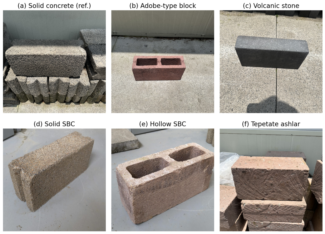
Five locally available sustainable wall materials were characterised (

Table 1. Test specimens and their measured physical and mechanical properties (mean of three specimens), in the order used throughout. “Ref.”: conventional concrete reference (baseline; thermal U from literature). “Alt.”: locally available sustainable alternative. “Struct.”: classed as suitable for structural use. Compressive strength converted from kg cm⁻² ($1\mathrm{kg}{\mathrm{cm}}^{-2}=0.098$ MPa).

Material	Role	Format	Density	Porosity	Absorp.	Comp.	Use
		cm	kg m−3	%	24 h %	MPa
Solid concrete	Ref.	40 × 20 × 15	∼2300	18.9	15.8	7.6	Non-str.
Adobe-type block	Alt.	40 × 20 × 12	∼1300	30.9	4.9	7.5	Struct.
Volcanic stone (recinto)	Alt.	24 × 12 × 6	∼1900	9.7	1.0	101	Struct.
SBC, solid	Alt.	38 × 18 × 12	∼1450	31.8	9.5	2.2	Non-str.
SBC, hollow	Alt.	40 × 20 × 15	∼1300	31.8	9.5	∼2.0 †	Non-str.
Tepetate ashlar	Alt.	45 × 25 × 20	∼1500	95 ‡	20.6	6.4	Non-str.

Densities are as-produced values used in the energy model. Porosity, absorption and compressive strength are from laboratory tests following the Mexican standards NMX-C-037-ONNCCE (water absorption) and NMX-C-036-ONNCCE (compressive strength); the concrete-reference values are for a lightweight concrete block. ^† Estimated from the solid SBC block (hollow not tested). ^‡ Anomalous (uncertain measurement). The SBC blocks contain ∼35% sargassum (producer data).

, Figure 1): two sargassum-based concrete (SBC) blocks—one solid and one hollow—incorporating dried sargassum as a partial aggregate (∼35% per the producer’s data) in a cement binder, and three local mineral alternatives (volcanic stone “recinto”, an adobe-type block and tepetate ashlar). From each material, a full-size ($1{\mathrm{m}}^2$) wall assembly was built for testing in the environmental chamber. A conventional solid-concrete wall is retained throughout as a literature-valued reference (baseline), because it is by far the most common wall material in the local social-housing stock and therefore the most suitable benchmark against which the sustainable alternatives are judged; it is not tested here.

3.2. Definitions: Conductivity, Resistance and Transmittance

The term “U-value” is used in the literature for several distinct quantities, which must be kept separate to interpret the results correctly. The symbols used throughout are therefore defined in

Table 2. Thermal quantities used in this study, based on ISO 6946 and ISO 9869-1. The transferable material property is the conductivity k; the directly measured quantity is the element resistance R; the input required by the energy model is the design air-to-air transmittance U.

Symbol	Quantity	Definition/How Obtained	Units
k	Intrinsic thermal conductivity	Material property; $k=e/R$ for tested thickness e	W m−1 K−1
R	Element (surface-to-surface) resistance	$R=\sum \Delta T_s/\sum q$ from the measured surface temperatures and heat flux (ISO 9869-1)	m2 K W−1
$R_{si},R_{se}$	Internal/external surface films	Standardised ISO 6946 values for horizontal flow, $0.13$/$0.04$	m2 K W−1
$h_i=1/R_{si}$	Internal surface coefficient	≈7.7 (from $R_{si}=0.13$); combined convective + radiative film	W m−2 K−1
U (design)	Air-to-air transmittance (model input)	$U=1/(R+R_{si}+R_{se})$; the value used in EnergyPlus	W m−2 K−1
$U_{a2a}$	Measured air-to-air transmittance	$U_{a2a}=\overline{q}/\Delta T_{\mathrm{air}}$; film-free cross-check	W m−2 K−1

, following ISO 6946 [17] and ISO 9869-1 [16]. Three quantities must be distinguished: the intrinsic conductivity k, a material property that is transferable across thicknesses; the element (surface-to-surface) resistance R, the quantity measured directly from the heat flux and the surface-to-surface temperature difference; and the design (air-to-air) transmittance $U=1/(R+R_{si}+R_{se})$, required as an input by EnergyPlus, which adds the standardised surface films. A second, independent transmittance—the measured air-to-air ratio $\overline{q}/\Delta T_{\mathrm{air}}$—is also reported as a film-free cross-check.

3.3. Thermal Characterisation (Heat-Flow-Meter Method)

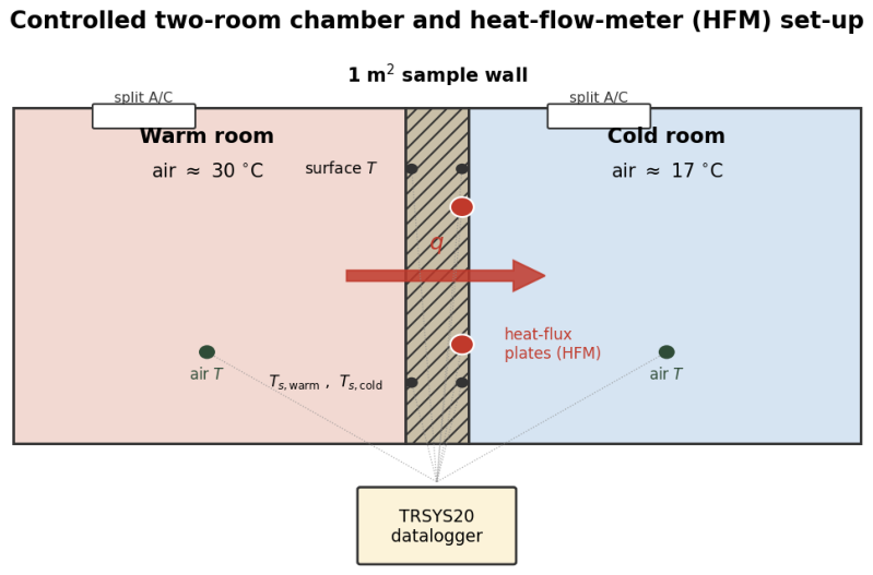
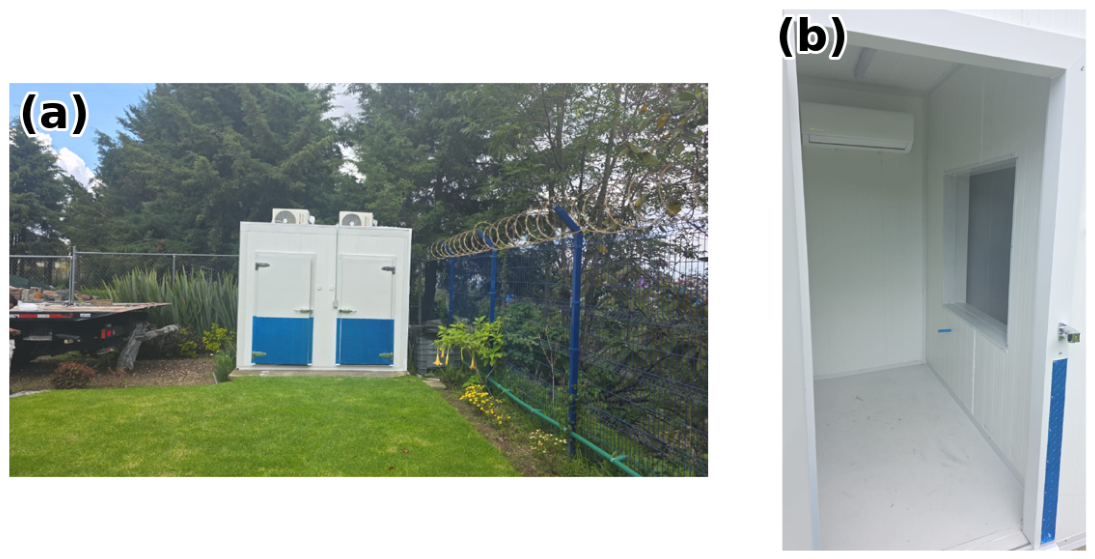
The resistance R and transmittance U of each assembly were estimated from heat-flux and temperature measurements taken with a Hukseflux TRSYS20 heat-flow-meter (HFM) system [49] in a purpose-built controlled environmental chamber. The chamber consisted of two adjoining conditioned rooms, each held by its own split air-conditioning unit at an average air temperature of 17 °C (cold room) and 30 °C (warm room). This gives an air-to-air difference of $\Delta T_{\mathrm{air}}=13$ K, used throughout the calculations. A $1{\mathrm{m}}^2$ sample wall is mounted in the dividing partition between the two rooms (Figure 2 and Figure 3).

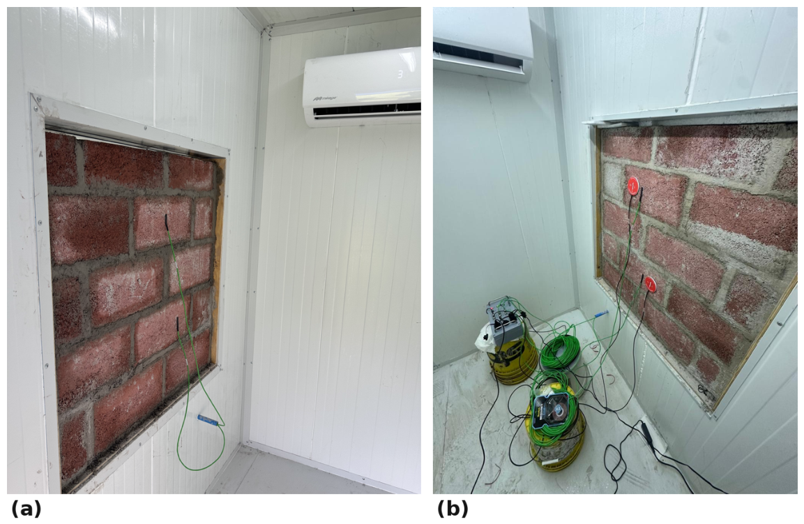
Two heat-flux plates were mounted on the cold-side face of the specimen at two representative locations, together with matched surface-temperature sensors on both faces and air-temperature sensors in each room (Figure 4); all channels were logged at a ten-minute interval. The two plates were separated by approximately $50\mathrm{cm}$ on the $1{\mathrm{m}}^2$ face—each set back at least $10\mathrm{cm}$ from the specimen edges to avoid two-dimensional perimeter effects, and centred over a different, representative region of the block—so that the simultaneous readings sample distinct heat-flow paths and their difference bounds the local spatial variation. ISO 9869-1 does not prescribe a fixed inter-plate spacing but requires each sensor to be located on a representative area away from edges, joints and thermal bridges; using two plates additionally exceeds the single-sensor minimum of the standard and quantifies the specimen heterogeneity, rather than being limited by channel availability. Each plate was fixed flush to the surface with double-sided adhesive tape—the mounting recommended for the TRSYS20 system and standard practice under ISO 9869-1—ensuring continuous contact with no intervening air gap, which limits the contact-resistance error that can otherwise inflate an HFM estimate substantially under poor surface contact or a low driving temperature difference [24,25]. The air-temperature sensors were placed about $1\mathrm{m}$ from the wall in each room. The louver of each split unit was fixed so that the supply air was deflected upstream and did not impinge directly on the wall, keeping the near-surface air movement low and repeatable. Because the cabin is outdoor-exposed, residual diurnal fluctuations remain, so the records are analysed with the ISO 9869-1 average method [16] rather than a single steady-state reading, and the standard’s acceptance criteria are enforced: a record longer than the 72 h minimum, agreement between successive analysis windows, and convergence of the running resistance to within the ISO 9869-1 tolerance, with plate agreement and temporal consistency checked jointly. A purely thermometric (air-temperature-based) estimate is available from the same records and is reported below as the independent air-to-air cross-check rather than as the primary result, because the HFM technique is the ISO 9869-1 reference method and measures the heat flux directly instead of inferring it from an assumed surface coefficient.

Two independent estimators of the transmittance are compared. In the first, the element (surface-to-surface) resistance is obtained from the measured surface temperature difference as $R=\sum \Delta T_s/\sum q$, giving the conductivity $k=e/R$; the wall transmittance then follows as the inverse of the total resistance, $U=1/(R+R_{si}+R_{se})$, using the standard surface films of ISO 6946 ($R_{si}=0.13$, $R_{se}=0.04{\mathrm{m}}^2{\mathrm{KW}}^{-1}$). These film resistances are prescribed by ISO 6946 for horizontal heat flow and differ between the two faces by design: the internal film ($R_{si}=0.13$, equivalently an internal surface coefficient $h_i=1/R_{si}\approx 7.7$ W m⁻² K⁻¹) is larger than the external one ($R_{se}=0.04$) because still indoor air exchanges heat less effectively than the wind-exposed outdoor surface. They are therefore adopted as standardised constants—the same values embedded in the EnergyPlus U—rather than fitted here. In the second estimator, which requires the measured air temperatures, an air-to-air transmittance $U_{a2a}=\overline{q}/\Delta T_{\mathrm{air}}$ is obtained directly from the heat flux and the air-to-air difference, without any surface-resistance assumption; the two estimates agreed to within about 5%, cross-validating the standardised films. This agreement also bounds the sensitivity to the film choice: the film resistance implied by the data (0.14–0.21 m² K W⁻¹, bracketing the standard $R_{si}+R_{se}=0.17$) moves U by only a few per cent, so a change in sensor position or in the assumed films does not materially alter the reported transmittances (Section 4). A dynamic grey-box estimator is additionally applied to corroborate the resistance from the transient and to recover the effective thermal mass [34,35].

3.3.1. Measurement Uncertainty

The uncertainty in the estimated transmittance is built up following the GUM framework [50] from two kinds of contribution: Type B (systematic, instrument) and Type A (statistical, repeatability). The Type B budget is propagated through the reduction $R=\sum \Delta T_s/\sum q$ and $U=1/(R+R_{si}+R_{se})$ (

Table 3. Uncertainty budget for the estimated transmittance U, following the GUM framework [50]. Type B (instrument) components are propagated through $R=\sum \Delta T_s/\sum q$ and $U=1/(R+R_{si}+R_{se})$; the Type A component is the measured repeatability. Values are typical relative magnitudes ($k=1$).

Source	Type	Typical Value
Heat-flux-plate calibration (on q)	B	$\pm 3\%$
Surface $\Delta T_s$ (sensors, $\Delta T_s\approx 4$–8 K)	B	$\pm 2$–$4\%$
Datalogger/acquisition	B	<0.5%
Combined Type B on R	B	$\pm 3.5$–$5\%$
propagated to U ($\times R/(R+R_{si}+R_{se})$)	B	$\pm 2$–$3\%$
Between-run/window repeatability	A	$\pm 1$–$6\%$
Combined standard uncertainty on $\mathit{U}$ ($\mathit{k}=\mathbf{1}$)	A ⊕ B	$\pm 3$–$7\%$

). The heat-flux plates carry a calibration uncertainty of about $\pm 3\%$ on q; the surface-to-surface temperature difference, of order 4–8 K, is measured to about $\pm 0.1$ K per sensor—i.e., $\pm 2$–$4\%$ relative, largest for the low-$\Delta T_s$ volcanic stone, while the datalogger contributes $<0.5\%$. Combined in quadrature, these give a Type B uncertainty of about $\pm 3.5$–$5\%$ on the element resistance R; because $U=1/(R+R_{si}+R_{se})$, this scales to the transmittance by the factor $R/(R+R_{si}+R_{se})\approx 0.55$–$0.65$, i.e., about $\pm 2$–$3\%$ on U. The Type A contribution is the between-run and window-to-window repeatability (∼$1$–$6\%$; Section 4), which additionally captures specimen mounting, boundary variability and—for the heterogeneous blocks—spatial sampling. The combined standard uncertainty, $u_c\left(U\right)/U=\sqrt{u_B^2+u_A^2}$, is therefore about $\pm 3$–$7\%$ ($k=1$): the plate calibration dominates the homogeneous, well-driven specimens, and the spatial repeatability the heterogeneous ones. This combined figure, rather than the fit residual, is reported throughout as the measurement uncertainty.

3.3.2. Scope and Representativeness of the Reported Values

The controlled chamber measures the block-scale assembly under a steady, known driving difference, capturing the block geometry and hollow cavities along the sensed heat-flow path. It does not reproduce every feature of a finished in-service wall: the reported values are element/path-level estimates for the block as tested, whereas mortar joints, plaster or render finishes and site workmanship would further modify the area-averaged U of a full wall, and the specimen is mounted in a partition aperture rather than exposed to real weather. Lateral heat exchange at the aperture perimeter was not separately quantified; the reduction assumes predominantly one-dimensional flow through the central sensed region, and the spread between the two plates is used to bound the local spatial variation (Section 5.5). For heterogeneous or hollow units, an area-weighted value is best obtained with distributed sensing or a guarded hot-box. The present figures are accordingly reported as controlled-chamber, path-representative estimates—not whole-wall in situ U-values—and are intended to be confirmed by in-service (in situ) measurement in future work.

3.4. Dynamic Grey-Box Analysis

To exploit the transient information in the sub-hourly records, the heat-flow series were also processed with a dynamic grey-box model, following the framework of Gori et al. [34,35]. The wall is represented by a lumped two-resistance, one-capacitance (2R1C) network: a single thermal-mass node at temperature $T_m$ with areal heat capacity C is connected to the measured internal and external surface temperatures $T_i$ and $T_e$ through resistances $R_1$ and $R_2$, with $R=R_1+R_2$ the element resistance. The energy balance at the mass node and the internal-surface heat flux q recorded by the HFM are

$$C{\displaystyle \frac{\mathrm{d}{T}_m}{\mathrm{d}t}}={\displaystyle \frac{T_i-T_m}{R_1}}+{\displaystyle \frac{T_e-T_m}{R_2}},q={\displaystyle \frac{T_i-T_m}{R_1}}.$$

(1)

Equation (1) is integrated at the logging step with the measured surface temperatures as inputs, so the model predicts the flux $\widehat{q}\left(t\right|\theta )$ for a parameter vector $\theta =\{R_1,R_2,C\}$.

For each specimen, the parameters $\theta =\{R_1,R_2,C\}$ are obtained by fitting the predicted flux $\widehat{q}\left(t\right|\theta )$ to the measured flux q, minimising the sum of squared residuals. Rather than reimplementing a full Bayesian inference, the minimisation is carried out deterministically with a Nelder–Mead simplex search on the log-parameters (to enforce positivity), restarted from several initial guesses to avoid local minima; the element resistance $R=R_1+R_2$, and hence $U=1/(R+R_{si}+R_{se})$, follow directly, together with the areal heat capacity C and the wall time constant $\tau =RC$. This deterministic dynamic fit is applied to every specimen and benchmarked against the ISO 9869 averaging value as a consistency check. Because it exploits the full transient rather than only the converged mean, it also yields a reliable resistance from records of limited duration, which is valuable for the shorter (73–76 h) runs that satisfy, but do not greatly exceed, the ISO 9869 minimum duration.

Because the sub-hourly residuals are serially correlated, the scatter of the fit alone understates the true uncertainty; accordingly, the between-run repeatability, rather than the fit residual, is adopted as the headline measurement uncertainty (Section 4). The effective heat capacity C and time constant $\tau$ are interpreted in Section 4.3.

3.5. Building Energy Modelling

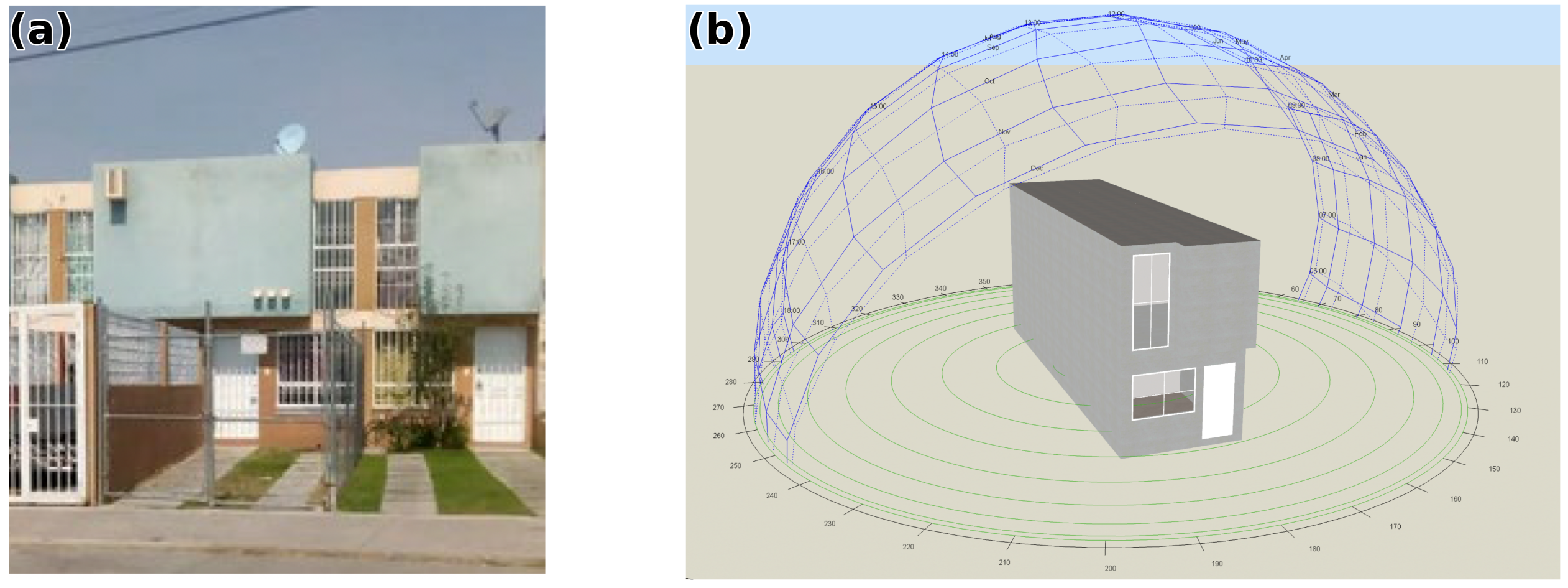
To connect the measured properties to energy performance, a whole-building dynamic simulation was carried out in EnergyPlus [37] through the DesignBuilder interface. The case study is the “Casa Los Héroes 1” prototype (Figure 5), a compact two-storey unit on a narrow (∼$63{\mathrm{m}}^2$) lot with load-bearing masonry walls, a concrete-slab roof and two main exposed façades, representative of the social-housing stock of the ZMVM; it has $79{\mathrm{m}}^2$ of built area ($39{\mathrm{m}}^2$ ground floor plus $40{\mathrm{m}}^2$ upper floor) and $73.45{\mathrm{m}}^2$ of conditioned floor area. The model is driven by a typical-meteorological-year weather file (EPW) derived from the ERA5 reanalysis (TMYx product) for the station nearest the case study, FES Cuautitlán in Cuautitlán Izcalli, State of Mexico (WMO 766700; 19.68° N, 99.20° W, $2251\mathrm{m}$ above sea level, GMT−6). At this altitude, the ZMVM has a temperate climate with a wide diurnal temperature swing and cool winters, so the building energy balance is heating-dominated with only marginal cooling—the regime in which the wall U-value most directly governs operational demand. Each wall material defines one simulation scenario; the other envelope elements, occupancy schedules, infiltration and internal gains are held fixed, so that differences in demand are attributable to the wall. Free-running comfort is evaluated with the ASHRAE 55 adaptive model [38], and the annual heating and cooling demand, the peak loads and the thermal-mass time lag are reported. These building-level outputs—rather than the U-value itself—are the quantities that housing energy-rating and subsidy tools, and designers, actually use, which is why the material properties are propagated to this scale.

Each wall is simulated twice: once with its literature thermal properties, providing a baseline (theoretical) demand, and once with its measured transmittance, so that the deviation introduced by measurement can be quantified directly at the building scale (Section 4). All five materials are carried through these paired simulations; for the hollow SBC block, the measured U is a web-biased upper bound (Section 5.5), so its simulated effect is likewise read as an upper estimate. A complete multi-scenario energy-and-life-cycle assessment built on these inputs is left to future work.

The prototype model was not calibrated against monitored indoor temperatures or metered energy. The building-level results are therefore reported as comparative scenario simulations that isolate the effect of the wall input (measurement-derived versus tabulated U) while holding all other model assumptions fixed, rather than as validated absolute predictions of demand. It is the difference between paired scenarios—not the absolute demand of any one scenario—that carries the conclusions of this paper; calibration against a monitored dwelling is identified as future work.

3.6. Open Data and Reproducibility

The workflow deliberately couples controlled-chamber estimation with whole-building simulation, so that the reusable contribution is not only the numbers but the method. To support reuse, the estimated properties are released as an open, simulation-ready material database (“Sustainable Walls—Measured U-values”): for each material, it provides the conductivity and transmittance together with ready-to-use EnergyPlus 23.1 (.idf) and DesignBuilder v2025 (.csv) material definitions, under a CC-BY-4.0 licence. The repository is version-controlled on GitHub (version 1.0.0, https://github.com/kerdan85/sustainable-walls-uvalues, accessed on 8 September 2026) and archived with a citable DOI on Zenodo (10.5281/zenodo.21897818); see also the Data Availability Statement.

4. Results

4.1. Thermal Properties

Table 4. Estimated versus literature thermal properties (HFM, ISO 9869-1). k: conductivity; U: wall transmittance; deviation relative to the literature estimate. Literature conductivities are standard tabulated design values [51] and domain-literature figures [5,45,46,47]. The conventional solid-concrete reference (first row) is listed at its literature value as the baseline; “—”: not estimated (the concrete reference is literature-only).

Material	${\mathit{k}}_{\mathbf{lit}}$	${\mathit{k}}_{\mathbf{est}}$	${\mathit{U}}_{\mathbf{lit}}$	${\mathit{U}}_{\mathbf{est}}$	Dev.
	W m−1K−1	W m−1K−1	W m−2K−1	W m−2K−1	%
Solid concrete (ref.)	1.74	—	4.19	—	—
Adobe-type block	0.50	0.38	2.44	2.07	$-15$
Volcanic stone	0.90	0.61	3.30	2.73	$-17$
SBC, solid	0.55	0.33	2.58	1.89	$-27$
SBC, hollow	0.45	0.53	1.99	2.21	$+11$
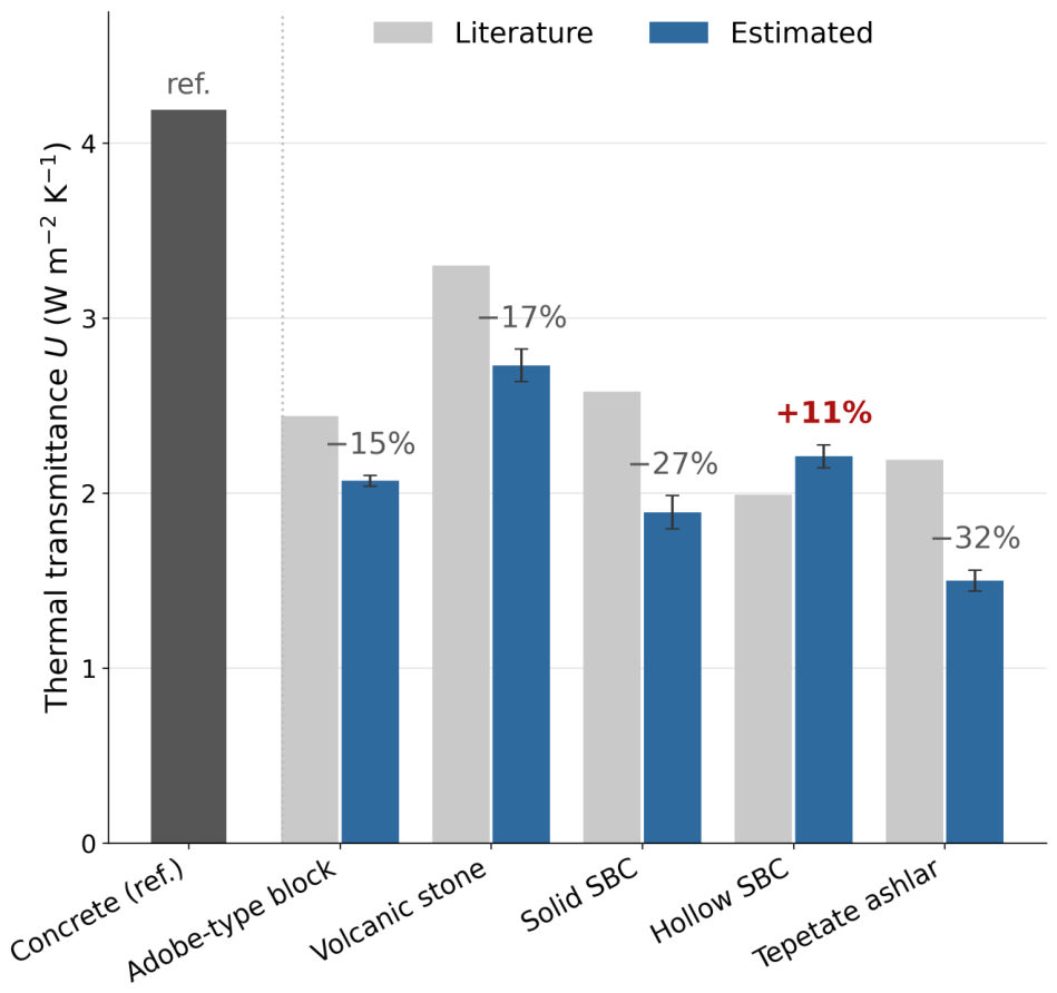
Tepetate ashlar	0.70	0.40	2.19	1.50	$-32$

reports the measured thermal conductivity and transmittance from the heat-flow-meter campaign against the literature-based estimates, together with the relative deviation. The literature conductivities ($k_{\mathrm{lit}}$) are the standard tabulated design values for building materials [51], supplemented for the local and novel materials by the domain literature—earthen blocks [45,46], volcanic stone and tuff [47], and sargassum-based concrete [5]—i.e., exactly the tabulated inputs an energy model would otherwise adopt in the absence of measurement. Each material is thus compared against the value that would actually be used for it in design, drawn material by material from the most specific published source available—the ISO 10456 generic building-material tables for the conventional concrete reference, and the domain-literature figures above for the earthen, volcanic and sargassum-based blocks—rather than against a single unrelated standard entry. The Mexican thermal-design tabulations used for norm compliance (NOM-020-ENER and the associated ONNCCE property tables) are themselves derived from the same international conventions and give values of the same order; where a local datasheet or norm value exists, it is preferred. The comparison matters precisely because no measured value existed for these local materials, so the tabulated figure—whatever its source—is what an energy model or rating tool would otherwise adopt. The first material completed (adobe-type block) was measured in two independent runs of over 72 h each, both satisfying the ISO 9869-1 duration, convergence ($\Delta R/R<5\%$ over the final 24 h) and temporal-consistency criteria. The two runs gave element resistances of $0.325$ and $0.303{\mathrm{m}}^2{\mathrm{KW}}^{-1}$ ($U=2.02$ and $2.12\mathrm{W}{\mathrm{m}}^{-2}{\mathrm{K}}^{-1}$), i.e., a repeatability of about 5%, and a combined estimate of $R\approx 0.31{\mathrm{m}}^2{\mathrm{KW}}^{-1}$, $k\approx 0.38\mathrm{W}{\mathrm{m}}^{-1}{\mathrm{K}}^{-1}$ and $U\approx 2.07\mathrm{W}{\mathrm{m}}^{-2}{\mathrm{K}}^{-1}$ (±5%), about 15% below the literature estimate. The block therefore performs better—has a lower transmittance—than assumed, though at $U\approx 2.1$ it is not, in absolute terms, an insulating wall. The between-run spread (∼5%) provides a more realistic measurement uncertainty than the within-run convergence alone.

The dense volcanic stone (recinto) was the most conductive of the sustainable set. The heat-flow-meter run on the $0.12\mathrm{m}$ wall (plates agreeing to 0.2%) gave an element resistance of $R\approx 0.20{\mathrm{m}}^2{\mathrm{KW}}^{-1}$, i.e., an intrinsic conductivity $k=e/R\approx 0.61\mathrm{W}{\mathrm{m}}^{-1}{\mathrm{K}}^{-1}$—about 32% below the literature estimate—and $U\approx 2.73\mathrm{W}{\mathrm{m}}^{-2}{\mathrm{K}}^{-1}$, about 17% below the literature value. Being a dense, solid stone, it remains the least insulating of the sustainable options measured, yet still measurably better than the handbook assumes.

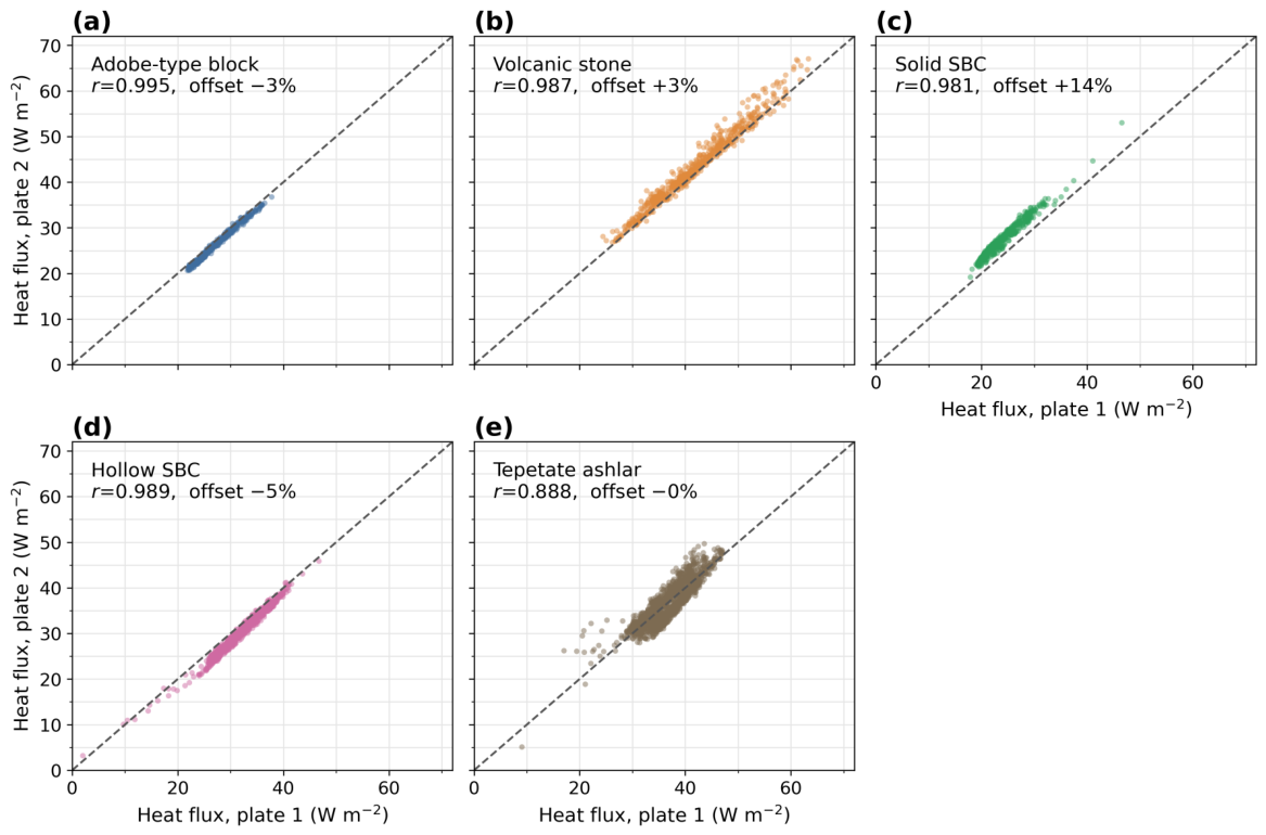
The solid sargassum-based block was the standout result: over 75 h it gave an element resistance of $0.36{\mathrm{m}}^2{\mathrm{KW}}^{-1}$, i.e., $k=0.33\mathrm{W}{\mathrm{m}}^{-1}{\mathrm{K}}^{-1}$ and $U=1.89\mathrm{W}{\mathrm{m}}^{-2}{\mathrm{K}}^{-1}$—about 40% below the literature conductivity and 27% below the literature transmittance, making it the most insulating material measured. This supports the expectation that the biomass fraction markedly lowers conductivity [5]. The two heat-flux plates differed by about 14% in recorded flux (Figure 6, against a few per cent for the other materials), indicating the pronounced spatial heterogeneity of the block, so the value carries an additional spatial uncertainty.

The tepetate ashlar (a light, consolidated volcanic tuff) was measured in two independent runs (212 h and 92 h) that agreed closely, with a between-run repeatability of about 3%. It gives an intrinsic conductivity $k\approx 0.40\mathrm{W}{\mathrm{m}}^{-1}{\mathrm{K}}^{-1}$, about 43% below the literature estimate, and, at its $0.20\mathrm{m}$ built thickness, a transmittance $U\approx 1.50\mathrm{W}{\mathrm{m}}^{-2}{\mathrm{K}}^{-1}$, about 32% below the literature value. This makes the tepetate the most insulating of the mineraloptions measured.

The hollow SBC block was the exception and is instructive. Estimated over 138 h at two sensor locations that gave element resistances of $0.27$ and $0.29{\mathrm{m}}^2{\mathrm{KW}}^{-1}$ (mean $R\approx 0.28{\mathrm{m}}^2{\mathrm{KW}}^{-1}$ at the $0.15\mathrm{m}$ block), it yields an effective conductivity $k\approx 0.53\mathrm{W}{\mathrm{m}}^{-1}{\mathrm{K}}^{-1}$ and $U\approx 2.21\mathrm{W}{\mathrm{m}}^{-2}{\mathrm{K}}^{-1}$ —about 11% above the tabulated value, the only material to exceed it.

Three factors explain the reversed sign, and together they make the hollow unit a cautionary case. First, the two heat-flux plates were mounted on the block face, which over a two-cell unit sits predominantly over the solid webs (the internal ribs that thermally bridge the cavities), so the estimate is weighted toward the conductive path and should be read as an upper bound; the ∼7% spread between the two locations already signals this strong internal heterogeneity. Second, tabulated effective values for hollow units credit the cavities as still air, whereas real cavities also transfer heat by convection and radiation.

The practical lesson is that a nominally identical-looking hollow block can depart from its tabulated value in either direction, and that heterogeneous units in particular require representative, multi-point sensing over both webs and cavities.

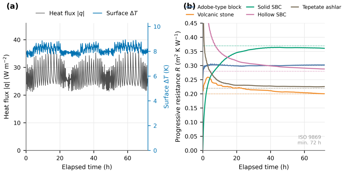
The underlying raw records are shown in Figure 7: the measured heat flux oscillates diurnally about a stable surface temperature difference (panel a), which is why the ISO 9869 average method—rather than a single reading—is used, and, plotted over a common 72 h window (panel b), the cumulative resistance of every material converges to a stable value well within the acquisition period.

Figure 6 plots the flux from the two plates against each other for each material, on a common set of axes so the magnitudes are directly comparable: the two plates track closely for most units (adobe, volcanic stone, tepetate and the hollow SBC block; $r=0.89$–$0.99$, mean plate offsets within ±5%), whereas the solid SBC block sits systematically above the 1:1 line (a $+14$% offset between plates), the signature of the biocomposite’s spatial heterogeneity discussed below. For the hollow SBC block, the plates agree in magnitude ($-5$% offset) yet yield element resistances differing by about 7%, because both plates sample the conductive web rather than the cavity—a point developed in the discussion.

This direct check of the raw two-sensor agreement, material by material, is a particular strength of this study. The measured values are collected in Table 4 and compared graphically in Figure 8.

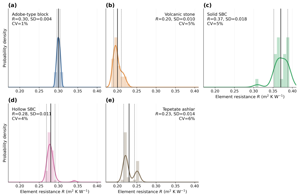
The repeatability of the measurement is quantified in Figure 9, which shows the distribution of the element resistance over 12 h rolling windows of each record. The window-to-window scatter is small—coefficients of variation of 1–6%—confirming that the reported values are stable, and is tightest and most symmetric for the homogeneous adobe block (mean $R=0.30$, CV 1%). The solid SBC block and the tepetate instead show visibly broader, slightly bimodal distributions, consistent with their spatial heterogeneity (also evident in the two-plate agreement, Figure 6). These distributions set a realistic measurement uncertainty of a few per cent on the reported R and U, in line with the ∼5% between-run repeatability of the replicated adobe block.

4.2. Dynamic Grey-Box Corroboration and Short-Record Robustness

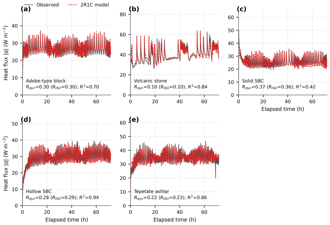
A distinctive strength of this work is that every block is analysed not only by ISO 9869 averaging but also with the dynamic grey-box method of Gori et al. [34,35], which draws on the full transient rather than only the converged mean. Fitting the 2R1C model—one lumped thermal-mass node between two resistances—to each block reproduces the measured heat flux (Figure 10); crucially, in every case, the identified dynamic resistance coincides with the ISO 9869 averaging value (Table 4) to within a few per cent, so the transmittance is robust to the reduction method. The goodness-of-fit spans $R^2\approx 0.4$–$0.9$: it is highest for the hollow SBC block ($R^2=0.95$, with $R_{\mathrm{dyn}}\approx 0.28{\mathrm{m}}^2{\mathrm{KW}}^{-1}$ reproducing the averaging value almost exactly), the tepetate ($0.86$) and the volcanic stone ($0.84$), and lowest for the solid SBC block ($0.42$)—the material with the most pronounced spatial heterogeneity (its $+14\%$ inter-plate offset), which a one-dimensional lumped model does not fully capture.

The excellent hollow-SBC fit is noteworthy: although its two plates sample a heterogeneous, web-dominated section, the transient is captured well and independently confirms the (upper-bound) resistance obtained by averaging.

For the adobe-type block, measured in two replicate runs, the 2R1C fit gives a well-defined element resistance ($R\approx 0.31{\mathrm{m}}^2{\mathrm{KW}}^{-1}$, $U\approx 2.08\mathrm{W}{\mathrm{m}}^{-2}{\mathrm{K}}^{-1}$) and a physically sensible areal heat capacity ($C\approx 120\mathrm{kJ}{\mathrm{m}}^{-2}{\mathrm{K}}^{-1}$, time constant $\approx 2.6\mathrm{h}$), confirming that the dynamic model captures the thermal-storage lag.

Critically for this campaign, because the dynamic estimator uses the entire transient rather than only the converged mean, it corroborates the element resistance from a shorter record than steady-state averaging alone would need. Several of the runs (73–76 h) satisfy but do not greatly exceed the ISO 9869 minimum duration, and the progressive resistance in Figure 7b is already flat well before the end of each test; applying the same 2R1C treatment to each material provides an independent, physics-based confirmation of the averaging value and so strengthens these shorter measurements rather than merely reproducing them. This is the practical reason the method is adopted here for all specimens, not only the long runs.

The scatter of the grey-box fit alone understates the true uncertainty, because the sub-hourly residuals are autocorrelated; the between-run repeatability (∼1–6%, Figure 9) is therefore adopted as the realistic measure of measurement uncertainty rather than the fit residual.

4.3. Thermal Inertia

Beyond the transmittance, the dynamic grey-box model returns the effective thermal mass: the areal heat capacity C and the associated time constant $\tau =RC$. It is important to read C correctly. A lumped model does not recover the total thermal mass of the wall but the effective thermal mass seen from the side on which the heat-flux plate is placed—here, the cold room—in the sense of the effective-thickness method of EN ISO 13786 [52], that is, the capacity of the wall as “seen” from the sensor side and coupled to that thermal zone. This is why the identified capacities appear modest for what are otherwise heavyweight masonry units, and it should be kept in mind both when interpreting the values and when transferring them into a whole-building tool such as EnergyPlus. For the adobe-type block the grey-box fit gives $C\approx 120\mathrm{kJ}{\mathrm{m}}^{-2}{\mathrm{K}}^{-1}$ ($\tau \approx 2.6\mathrm{h}$); applying the same 2R1C fit to the other blocks, the identified time constants (of order 2–4 h) place the solid SBC block as the most thermally massive of the measured set—the longest response—while the dense volcanic stone combines a low resistance with appreciable mass. Because $\tau$ is formed from this effective (not total) capacity, it too should be read as a zone-side response time rather than a full-wall decrement lag. This inertia is what damps indoor temperature swings and can matter as much as the transmittance for adaptive comfort. Two further caveats apply. First, because the controlled chamber holds near-steady air setpoints, the dynamic excitation is modest, so the heat capacity is identified with more uncertainty than the transmittance—the chamber is optimised for U, not for the thermal mass, and a ramped or periodic boundary protocol would sharpen C. Second, a conventional decrement time-lag (the delay between an external temperature peak and the inner response) is not cleanly recoverable under these deliberately steady conditions and is better obtained in situ or with a driven cycle.

A material-by-material comparison of the dynamic and averaging resistances is provided in Figure 10, where each panel annotates $R_{\mathrm{dyn}}$ against $R_{\mathrm{ISO}}$; in every case, the two agree to within a few per cent, confirming that the transmittance is independent of the reduction method.

4.4. Energy Simulation with Measured Versus Literature Inputs

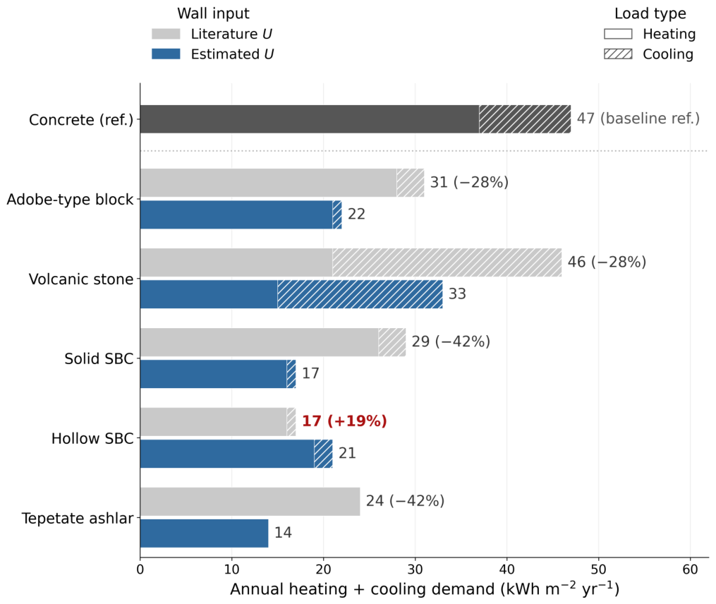
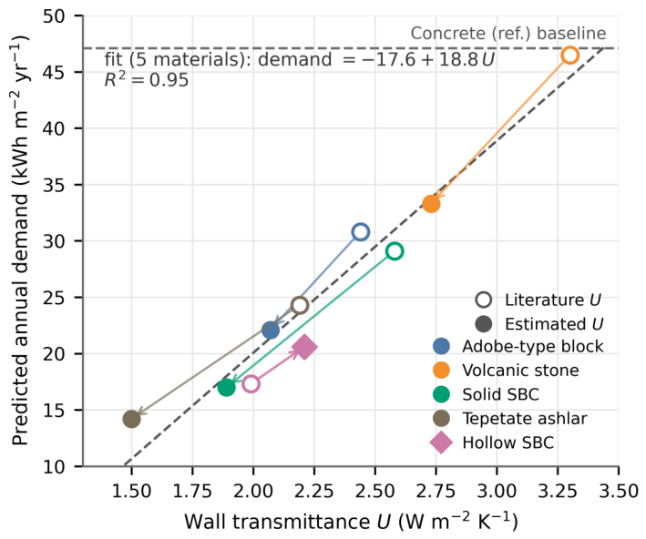
Feeding the measurement-derived transmittances into the whole-building model lowers the predicted annual heating-plus-cooling demand of the four solid or homogeneous walls by 28–42% relative to the literature-based baseline; the hollow SBC block—the only material estimated above its tabulated value—is the exception, its demand rising by 19% (

Table 5. Simulated annual demand of the social-housing case study for each wall (EnergyPlus, typical meteorological year), with the literature transmittance (baseline) and the estimated transmittance. U: wall transmittance; Demand: annual heating-plus-cooling per conditioned floor area; $\Delta$: change from baseline; comfort under the ASHRAE 55 adaptive model with the estimated U. Only the wall material is varied between runs.

Wall Material	${\mathit{U}}_{\mathbf{lit}}$	${\mathit{U}}_{\mathbf{est}}$	Demandlit	Demandest	$\mathbf{\Delta }$	Comfort
	W m−2K−1		kWh m−2 yr−1		%	%
Solid concrete (ref.)	4.19	—	47.1	—	—	50.3
Adobe-type block	2.44	2.07	30.8	22.1	$-28$	47.7
Volcanic stone	3.30	2.73	46.5	33.3	$-28$	60.1
SBC, solid	2.58	1.89	29.1	17.0	$-42$	50.9
SBC, hollow †	1.99	2.21	17.3	20.6	$+19$	50.6
Tepetate ashlar	2.19	1.50	24.3	14.2	$-42$	39.1

^† The hollow SBC block is the only material whose estimated U (2.21) exceeds its tabulated value (1.99); consistently, it is the only wall whose estimated transmittance raises the predicted demand (by $+19\%$), opposite to the other four. Because its web-biased estimate is an upper bound (Section 4), this $+19\%$ is itself an upper estimate of the effect.

, Figure 11). This is the direct pay-off of measuring, rather than assuming, the input, and its sign follows the sign of the measurement gap. As a common yardstick, a conventional solid-concrete wall (kept at its literature value) gives a baseline demand of about 47 kWh m⁻² yr⁻¹; every sustainable material sits well below this benchmark.

Each material was simulated twice—once with its literature properties (baseline) and once with its measured U—holding all other envelope elements, occupancy schedules, infiltration and internal gains fixed, so that the difference in demand is attributable solely to the wall. For the four walls that insulate better than assumed, the tabulated heating-dominated demand of $24$–$47\mathrm{kWh}{\mathrm{m}}^{-2}{\mathrm{yr}}^{-1}$ fell to $14$–$33\mathrm{kWh}{\mathrm{m}}^{-2}{\mathrm{yr}}^{-1}$ with the measured transmittance, an absolute saving of roughly 9–13 kWh m⁻² yr⁻¹ per wall; the reduction is largest for the two materials with the widest measurement gap—the solid SBC block and the tepetate ashlar (both $-42\%$).

For the hollow SBC block, the direction reverses in step with its transmittance: demand rises from $17.3$ to $20.6\mathrm{kWh}{\mathrm{m}}^{-2}{\mathrm{yr}}^{-1}$ ($+19\%$), a ∼3 kWh m⁻² yr⁻¹ increase—though, since the measured U is a web-biased upper bound, this is an upper estimate of the effect.

The change is carried almost entirely by the heating term, consistent with the temperate, heating-relevant climate; the free-running comfortable-hour share is essentially unchanged (e.g., volcanic stone $56.5\to 60.1\%$; hollow SBC $50.9\to 50.6\%$). Peak heating loads move in step, easing (or, for the hollow unit, marginally increasing) equipment sizing.

The direction is unambiguous and design-relevant: where the wall insulates better than the handbook assumes, a model built on tabulated inputs overestimates the demand—by up to two-fifths of the predicted total—while for the hollow unit it underestimates it; either way, the bias is large enough to alter the apparent performance ranking of the materials and the sizing of the heating system. The consistency of the sign, material by material, with the sign of the measurement gap is itself evidence that the effect is real and not an artefact.

4.5. Sensitivity of Predicted Demand to the Transmittance Input

The five materials, together with their literature baselines, give ten (U, demand) points that map how strongly the model output depends on the wall input (Figure 12). The predicted annual demand is almost perfectly linear in the wall transmittance ($\mathrm{demand}\approx -17.6+18.8U$, $R^2=0.95$): every unit of transmittance ($1\mathrm{W}{\mathrm{m}}^{-2}{\mathrm{K}}^{-1}$) carries about 19 kWh m⁻² yr⁻¹ of predicted demand, so a $0.5$ W m⁻² K⁻¹ error in the assumed U—well within the 15–32% gap estimated here—displaces the prediction by roughly 9 kWh m⁻² yr⁻¹. The hollow SBC block sits on the same line: its higher estimated U moves it up the relationship, raising the demand by $+19\%$, so the linear response holds in both directions.

Two features sharpen this. First, the response is amplified: the fractional change in predicted demand exceeds the fractional change in U by a factor of 1.3–1.9 (mean $\approx 1.6$), because, in this mild, heating-dominated climate, the net demand is a small residual between comparable gains and losses, so a given relative error in the wall loss is magnified in the delivered energy—a tabulated U that is 15–32% too high inflates the predicted demand by 28–42%. Second, the bias also propagates to the peak heating load: substituting the measured U lowered the design heating load by 19–30% (from 62–86 to 44–69 W m⁻²), which feeds directly into equipment sizing. Measured inputs therefore sharpen not only the energy estimate but the plant capacity and the comparative ranking on which specification decisions rest.

5. Discussion

This study set out to replace tabulated envelope inputs with estimates derived from direct measurements and to test what that changes. Three findings frame the discussion: the estimated transmittances depart substantially from the literature values—materially lower for four of the five materials, and higher for one; the dynamic grey-box method corroborates them—robustly, even for short records; and the resulting bias in predicted energy demand is large enough to matter for design and for the ranking of materials. These are taken in turn, followed by the geometric and heterogeneity effects that condition the measurements, and the study’s limitations.

5.1. Estimated Transmittance and Implications for Energy Modelling

For the four materials with lower estimated U-values the departure from the literature estimate is one-directional: the tabulated conductivity overestimates the value of the as-built assembly, by 24–45% in k and 15–34% in U.

Three general mechanisms explain why a tabulated input can misstate the real performance. First, similarly-looking materials can have quite different thermophysical properties, so when no detailed data are available it is difficult to select a value that is representative of a specific construction from a generic table. Second, tabulated conductivities and manufacturer specifications are usually derived from controlled laboratory tests, which need not represent how the material performs in situ over time—as affected by moisture (from rain, from the indoor use of the space, or retained from the construction process), by density as produced, and by ageing. Third, for hollow units, tabulated values are both scarcer and harder to derive because the air cavities must themselves be characterised; the hollow SBC block is precisely this case, exceeding its tabulated value by ∼11% (Section 4 and Section 5.5). For hollow, heterogeneous units, the discrepancy can therefore run in either direction, which is itself an argument for measurement.

For the four assemblies that insulate better than assumed, an energy model fed with literature inputs overestimates the heating demand; substituting the measured U removes this conservative bias and lowers the predicted demand for the affected walls in the energy model (Section 4.4).

The solid sargassum-based block is the clearest case: its measured conductivity ($k\approx 0.33\mathrm{W}{\mathrm{m}}^{-1}{\mathrm{K}}^{-1}$, $U\approx 1.89\mathrm{W}{\mathrm{m}}^{-2}{\mathrm{K}}^{-1}$) is the lowest of the set and about 40% below the tabulated value, consistent with the hypothesis that the biomass fraction reduces conductivity [5].

Sargassum is a pelagic macroalga that, since around 2011, has beached in massive quantities on Caribbean and West-African coasts, imposing high ecological and economic costs [4,48]; incorporating the dried biomass as a partial aggregate is one of several routes proposed to valorise this waste stream while lowering the conductivity of the masonry [5]. This result therefore strengthens the case for the thermal performance of sargassum-based blocks—their lower transmittance relative to conventional units. Thermal performance alone, however, does not establish fitness for social housing: for a biomass-containing cementitious block, the durability, moisture and biological stability, fire behaviour, structural capacity and transport logistics of the raw sargassum must each be assessed separately before adoption, and these lie outside the thermal scope of the present study. The thermal advantage reported here is thus a necessary, but not a sufficient condition, to be weighed alongside those factors. Because sargassum is not a widely known construction material outside the affected regions, this context is noted explicitly for the international reader.

5.2. Effect on Predicted Energy Use

The measurement bias is design-relevant rather than academic. Propagated through the whole-building model, the measured transmittances lower the predicted annual heating-plus-cooling demand of the four walls by 28–42%—roughly 9–13 kWh m⁻² yr⁻¹—relative to the tabulated baseline (Table 5, Figure 11). The effect is not a uniform offset: it scales with each material’s measurement gap, so the solid SBC block and the tepetate ashlar, the two with the widest conductivity discrepancy, show the largest demand reductions ($-42\%$), whereas the adobe and volcanic assemblies fall by $-28\%$.

Because the reduction is material-specific, it compresses the spread between the assemblies and can therefore reorder their apparent ranking rather than merely rescale it: a designer optimising on tabulated inputs would both over-predict absolute demand and risk mis-ordering the options. The change is carried almost entirely by the heating term, as expected in this heating-dominated highland climate, while the free-running comfortable-hour share is essentially preserved, so the benefit surfaces as lower delivered energy and smaller heating plant rather than as a comfort penalty.

This also delimits when tabulated inputs are, and are not, defensible. The predicted demand tracks the wall U almost linearly and with amplified sensitivity (Section 4.5) precisely because the wall is a dominant loss path and the net demand is a small residual in this mild climate; under those conditions, a tabulated U error propagates—magnified—into the result, and measurement is warranted. Where the wall is a minor loss path (highly insulated envelopes, small wall-to-floor ratios) or the climate is cooling-dominated with large solar and internal gains, the same absolute U error moves the prediction far less, and handbook values may suffice. The materials and climate studied here fall squarely in the first regime, which is also the regime of most concern for low-income housing, where heating energy is a direct cost burden.

5.3. Implications for Practice and Policy

The consequence of this bias is not confined to a research estimate, because in social housing the envelope inputs travel directly into the instruments that allocate finance and certify performance. In Mexico, dwellings are rated and made eligible for green-mortgage and subsidy support through simulation-based tools—SISEVIVE-Ecocasa and its DEEVi engine, linked to INFONAVIT’s Hipoteca Verde, the Vivienda Sustentable NAMA and NOM-020-ENER compliance—and these tools draw the wall properties from tabulated material libraries. The results imply that, for the local and novel materials examined, those libraries misstate the transmittance and therefore the predicted demand—overstating it for the four lower-U materials and understating it for the hollow unit. For the four, a rating built on those libraries would credit the dwelling with less envelope performance than it actually has, penalising precisely the low-carbon local materials that such programmes intend to promote.

Two practical implications follow. First, the effect is material-specific ($-15$ to $-34\%$ in U) and redistributes between heating and cooling, so it can change which wall a designer or evaluator would select, not merely the magnitude of a single estimate; a recent field study of prefabricated dwellings likewise found the theory–measurement gap large enough to reverse the calculated ranking of envelopes [53], so measured inputs are decision-relevant, not cosmetic. Second, the workflow demonstrated here—first characterise the material in a controlled chamber, then feed the validated value into the same simulation engine that practitioners and rating tools already use—is transferable to any locally available material, and the accompanying open, simulation-ready database is intended to let designers, evaluators and researchers adopt measured inputs directly.

Although the specific instruments named above are Mexican, the mechanism is general and the message is not confined to Mexico or to social housing: wherever building energy ratings, compliance checks or incentive schemes run simulations on tabulated material libraries—and many national building regulations additionally set a maximum permissible wall U-value—a biased library input propagates into the rating, the compliance verdict and the subsidy decision. Social housing is foregrounded here because it is the segment in which low-carbon local and novel materials are most actively trialled and in which heating energy is a direct cost burden for occupants, so an input bias has the sharpest welfare consequences; nevertheless, the same argument applies to any stock and climate in the sensitivity regime identified above.

5.4. Value of the Controlled-Chamber and Dynamic Grey-Box Approach

The controlled two-room chamber imposes a steady, known driving difference and measures the block-scale assembly under near-one-dimensional flow—capturing the block cavities and real geometry along the sensed path, though not the mortar joints, renders and workmanship of a finished wall, so the reported values are element-/path-level rather than whole-wall in situ figures (Section 3). Two independent transmittance estimates were compared: the surface-to-surface resistance combined with the ISO 6946 surface films, and the air-to-air ratio $\overline{q}/\Delta T_{\mathrm{air}}$ obtained from the constant chamber temperatures. They agreed to within about 5%, which cross-validates the result and shows that the standard $R_{si}/R_{se}$ assumption was adequate here; the implied real film resistance (0.14–0.21 ${\mathrm{m}}^2{\mathrm{KW}}^{-1}$) bracketed the standard value of $0.17{\mathrm{m}}^2{\mathrm{KW}}^{-1}$.

The dynamic grey-box fit added value beyond a single number: it reproduced the averaging resistance, recovered a physically sensible effective thermal mass ($C\approx 120\mathrm{kJ}{\mathrm{m}}^{-2}{\mathrm{K}}^{-1}$, for the replicated adobe block) and fitted the transient heat flux far better than a static relation. The scatter of the fit alone must be read with care: with sub-hourly, autocorrelated residuals, it is over-confident, and the between-run repeatability (∼1–6%) is a more realistic measure of uncertainty.

Equally important, because the estimator uses the whole transient rather than only the converged mean, it extracts a reliable resistance from records of limited duration; this is why it is applied to every specimen and not just the long runs. Several of the tests (73–76 h) meet but do not greatly exceed the ISO 9869 minimum, and the dynamic method provides an independent, physics-based confirmation that strengthens those shorter measurements—a practical advantage when throughput or specimen availability limits how long each wall can occupy the chamber.

5.5. Effect of Specimen Heterogeneity

Material heterogeneity proved consequential. The solid sargassum block showed a ∼14% offset between the two heat-flux plates (Figure 6), against a few per cent for the other materials. This reveals the spatial heterogeneity of the biocomposite (uneven biomass and aggregate) and adds a spatial uncertainty. It argues for multi-point or distributed sensing on heterogeneous materials. A related effect concerns the most conductive assembly: the volcanic stone. Its surface-to-surface temperature difference was small (∼$4\mathrm{K}$ of the $13\mathrm{K}$ air difference), because the wall resistance is comparable to the surface films. Testing conductive assemblies therefore benefits from a larger imposed $\Delta T$ to preserve the signal-to-noise ratio.

A special case of this heterogeneity is the hollow SBC block, the only material whose estimated transmittance ($U\approx 2.21\mathrm{W}{\mathrm{m}}^{-2}{\mathrm{K}}^{-1}$) exceeded its tabulated value ($1.99\mathrm{W}{\mathrm{m}}^{-2}{\mathrm{K}}^{-1}$, $+11\%$); since its grey-box fit was in fact the best of the set ($R^2=0.94$), the reversal is physical rather than an artefact. It arises because the two plates, mounted on the block face, sit predominantly over the solid webs that thermally bridge the cavities, so a one-dimensional reading over them samples the conductive path and overestimates the area-averaged conductance—the reported value is therefore an upper bound, and the ∼7% spread between the two plate locations already signals this.

This upper-bound character can be made quantitative with the standard reduced (effective) resistance $R_{\mathrm{pr}}=A/{\sum }_i(A_i/R_i)$ used for constructions of non-uniform resistance [17]. Using the measured block geometry (two cavities; face-shells ≈ $3\mathrm{cm}$ and a web face-area fraction $\approx 0.3$) and treating each block as two parallel paths—the solid webs and the cavities (face-shells in series with an unventilated air layer, $R_{\mathrm{air}}\approx 0.18{\mathrm{m}}^2{\mathrm{KW}}^{-1}$), with the independently measured solid-SBC conductivity ($k=0.33\mathrm{W}{\mathrm{m}}^{-1}{\mathrm{K}}^{-1}$)—gives an effective $U\approx 1.7\mathrm{W}{\mathrm{m}}^{-2}{\mathrm{K}}^{-1}$ for the hollow SBC block. This lies well below the two-plate value (2.21), confirming that plates sitting over the webs return an upper bound and that the true area-weighted transmittance is lower. For the adobe-type hollow block the same calculation gives $\approx 2.2\mathrm{W}{\mathrm{m}}^{-2}{\mathrm{K}}^{-1}$, within about 7% of the measured 2.07. For the solid and homogeneous blocks, no internal thermal bridges exist, so the reduced resistance coincides with the measured element resistance.

Compounding it, tabulated effective values credit the cavities as still air, whereas real cavities also transfer heat by convection and long-wave radiation (the ISO 6946 cavity resistance is modest [17]), and two-dimensional bridging through the webs raises the effective conductance above a layered handbook estimate—so hollow units, unlike solid ones, can measure above their tabulated value [23,29].

The lesson is that heterogeneous hollow units need multi-point sensing over both webs and cavities (or a guarded hot-box) for an area-weighted U, and that their tabulated inputs cannot be assumed conservative.

Propagated through the building model, this upper-bound U is the only one to raise the predicted demand (by $+19\%$, versus the $-28$ to $-42\%$ of the other four; Table 5)—so the sign of the building-level effect tracks the sign of the measurement gap material by material, which is itself a consistency check on the whole workflow. Because the estimate is an upper bound, the true increase is likely smaller, and obtaining the area-weighted value is the natural next step.

5.6. Limitations

This study reports the estimated thermal transmittance of all five sustainable wall materials; for the hollow SBC block, the two-plate estimate is a web-biased upper bound (Section 5.5), which is why its area-weighted value, and its energy simulation, are left to a distributed-sensor follow-up. The transmittances correspond to a controlled chamber rather than to real in-service exposure (weather, driving rain, solar gain), although the measured element resistance is a transferable property.

The reported measurement uncertainty is the window-to-window repeatability (∼1–6%), taken across runs and rolling windows rather than from the fit residual. A single specimen per material was tested; replicate specimens will further tighten the material-level uncertainty.

Three further limitations should be read alongside the results. First, the reported transmittances are element-/path-level values for the block as tested: the mortar joints, plaster or render finishes and workmanship of a finished wall, and the area-weighting over webs and cavities for the hollow units, remain to be captured by distributed, in-service (in situ) measurement. Second, the specimen is mounted in a partition aperture rather than exposed to weather, and lateral heat exchange at the aperture perimeter was not separately quantified. Third, the building energy results are comparative scenario simulations from an uncalibrated prototype: their purpose is to translate the measured input change into a demand change, not to predict any dwelling’s absolute consumption, and calibration against monitored indoor temperatures and metered energy is left to future work.

6. Conclusions

This paper reported estimates—derived from controlled-chamber heat-flux and temperature measurements—of the thermal transmittance of sustainable wall materials for social housing in the Mexico City Metropolitan Area, obtained with a heat-flow-meter system in a purpose-built controlled two-room chamber and reduced with three independent estimators (ISO 9869-1 averaging, direct air-to-air, and a dynamic grey-box). The central result is the size and direction of the gap between the measurement-derived and the tabulated properties, and its agreement with the wider measurement literature:

• For four of the five materials, the as-built conductivity was 24–45% below the tabulated design value (15–34% in U): the handbook figure overstates the transmittance of the real assembly (adobe $-15\%$, volcanic stone $-17\%$, solid SBC $-27\%$, tepetate $-32\%$ in U). The hollow SBC block was the exception, exceeding its tabulated value by ∼11%—so the gap can run in either direction, especially for heterogeneous, hollow units, which is itself an argument for measurement. The solid SBC block was the most insulating material estimated ($k\approx 0.33\mathrm{W}{\mathrm{m}}^{-1}{\mathrm{K}}^{-1}$, $U\approx 1.89\mathrm{W}{\mathrm{m}}^{-2}{\mathrm{K}}^{-1}$), consistent with a conductivity-lowering effect of the biomass fraction.
• This measured-below-tabulated gap is consistent with the international evidence for conventional construction. The large heat-flux campaign of Li et al. found in situ solid-wall U-values about a third below the standard assumption [22]; the BRE in situ survey of English housing reached the same conclusion at stock scale [54]; a recent review across conventional and bio-based envelopes reports the theory–measurement gap to be significant and largest for concrete and brick [23]; and controlled and field comparisons of measured against calculated U, including campaigns that propagate the measured value into predicted heating demand, report deviations of the same order and sign [18,19,40]. The contribution here is to extend this evidence from conventional walls to locally available and novel sustainable materials, for which measured transmittances were essentially absent, and to show that the bias runs the same way and is large.
• The two independent transmittance estimators (surface-to-surface with ISO 6946 films and direct air-to-air) agreed to within about 5%, and the dynamic grey-box model reproduced the same resistance while recovering a physically sensible effective thermal mass ($C\approx 120\mathrm{kJ}{\mathrm{m}}^{-2}{\mathrm{K}}^{-1}$ for the replicated adobe block) and fitting the transient far better than a static relation. The reported measurement uncertainty is the between-run repeatability (∼1–6%).
• Specimen geometry and material heterogeneity were shown to matter: the conductivity, not the as-built transmittance, is the transferable property when the tested thickness differs from the design wall, and heterogeneous biocomposites require multi-point sensing to bound their spatial uncertainty.
• Propagated through a whole-building EnergyPlus model of a social-housing archetype, the measured transmittances lowered the predicted annual heating-plus-cooling demand by 28–42% (about 9–13 kWh m⁻² yr⁻¹) for the four walls that insulate better than assumed, while the hollow SBC block—the one material estimated above its tabulated value—instead raised it by 19%. The building-level effect thus follows the sign of the measurement gap material by material, and its magnitude is large enough to alter the apparent ranking of the assemblies, not merely their absolute demand—so measured inputs improve both the accuracy and the comparative reliability of the energy model.

In summary, for four of the five materials, the controlled-chamber U was 15–34% below the tabulated value and, for the hollow SBC block, ∼11% above it, and propagating these values shifted the predicted annual heating-plus-cooling demand by $-28$ to $+19\%$—enough to reorder the assemblies. For social housing in the ZMVM, the implication is direct: energy models, and the ratings and subsidies built on them, should use measured rather than tabulated transmittances for these local materials. The values are reported as controlled-chamber, element-level estimates, to be confirmed by in-service measurement and by area-weighted sensing for the hollow units; to that end, the measured properties are released as an open, simulation-ready material database that future campaigns can extend.

References

1. United Nations Environment Programme. 2022 Global Status Report for Buildings and Construction: Towards a Zero-Emission, Efficient and Resilient Buildings and Construction Sector; Technical Report; UNEP: Nairobi, Kenya, 2022. [Google Scholar]
2. International Energy Agency. Buildings—Energy System; Technical Report; IEA: Paris, France, 2023; Available online: https://www.iea.org/energy-system/buildings (accessed on 12 July 2026).
3. Röck, M.; Saade, M.R.M.; Balouktsi, M.; Rasmussen, F.N.; Birgisdóttir, H.; Frischknecht, R.; Habert, G.; Lützkendorf, T.; Passer, A. Embodied GHG emissions of buildings—The hidden challenge for effective climate change mitigation. Appl. Energy 2020, 258, 114107. [Google Scholar] [CrossRef] [Scilit]
4. Wang, M.; Hu, C.; Barnes, B.B.; Mitchum, G.; Lapointe, B.; Montoya, J.P. The great Atlantic Sargassum belt. Science 2019, 365, 83–87. [Google Scholar] [CrossRef] [Scilit] [PubMed]
5. Rosas-Díaz, F.; Juárez-Alvarado, C.A.; Chen, M.; Ye, Y.; Myers, R.J.; Jiang, D. Biomass-based concrete could effectively decarbonize buildings in Mexico. Resour. Conserv. Recycl. 2025, 219, 108264. [Google Scholar] [CrossRef] [Scilit]
6. Secretaría de Energía (SENER). NOM-020-ENER-2011: Eficiencia Energética en Edificaciones—Envolvente de Edificios para uso Habitacional; Technical Report; Diario Oficial de la Federación: Mexico City, Mexico, 2011.
7. Comisión Nacional de Vivienda (CONAVI); GIZ. SISEVIVE-Ecocasa: Sistema de Evaluación de la Vivienda Verde—Metodología y herramienta DEEVi; Technical Report; CONAVI: Mexico City, Mexico, 2015.
8. Pomponi, F.; Moncaster, A. Embodied carbon mitigation and reduction in the built environment—What does the evidence say? J. Environ. Manag. 2016, 181, 687–700. [Google Scholar] [CrossRef] [Scilit] [PubMed]
9. Cabeza, L.F.; Rincón, L.; Vilariño, V.; Pérez, G.; Castell, A. Life cycle assessment (LCA) and life cycle energy analysis (LCEA) of buildings and the building sector: A review. Renew. Sustain. Energy Rev. 2014, 29, 394–416. [Google Scholar] [CrossRef] [Scilit]
10. Asdrubali, F.; D’Alessandro, F.; Schiavoni, S. A review of unconventional sustainable building insulation materials. Sustain. Mater. Technol. 2015, 4, 1–17. [Google Scholar] [CrossRef] [Scilit]
11. Schiavoni, S.; D’Alessandro, F.; Bianchi, F.; Asdrubali, F. Insulation materials for the building sector: A review and comparative analysis. Renew. Sustain. Energy Rev. 2016, 62, 988–1011. [Google Scholar] [CrossRef] [Scilit]
12. Aditya, L.; Mahlia, T.M.I.; Rismanchi, B.; Ng, H.M.; Hasan, M.H.; Metselaar, H.S.C.; Muraza, O.; Aditiya, H.B. A review on insulation materials for energy conservation in buildings. Renew. Sustain. Energy Rev. 2017, 73, 1352–1365. [Google Scholar] [CrossRef] [Scilit]
13. Laborel-Préneron, A.; Aubert, J.E.; Magniont, C.; Tribout, C.; Bertron, A. Plant aggregates and fibers in earth construction materials: A review. Constr. Build. Mater. 2016, 111, 719–734. [Google Scholar] [CrossRef] [Scilit]
14. Pisello, A.L. State of the art on the development of cool coatings for buildings and cities. Sol. Energy 2017, 144, 660–680. [Google Scholar] [CrossRef] [Scilit]
15. Bai, M.; Wu, Y.; Xiao, J.; Ding, T.; Yu, K. Workability and hardened properties of 3D printed engineered cementitious composites incorporating recycled sand and PE fibers. J. Build. Eng. 2023, 71, 106477. [Google Scholar] [CrossRef] [Scilit]
16. ISO 9869-1:2014; Thermal Insulation—Building Elements—In-Situ Measurement of Thermal Resistance and Thermal Transmittance—Part 1: Heat Flow Meter Method. International Organization for Standardization (ISO): Geneva, Switzerland, 2014.
17. ISO 6946:2017; Building Components and Building Elements—Thermal Resistance and Thermal Transmittance—Calculation Methods. International Organization for Standardization: Geneva, Switzerland, 2017.
18. Ficco, G.; Iannetta, F.; Ianniello, E.; d’Ambrosio Alfano, F.R.; Dell’Isola, M. U-value in situ measurement for energy diagnosis of existing buildings. Energy Build. 2015, 104, 108–121. [Google Scholar] [CrossRef] [Scilit]
19. Evangelisti, L.; Guattari, C.; Gori, P.; de Lieto Vollaro, R. In situ thermal transmittance measurements for investigating differences between wall models and actual building performance. Sustainability 2015, 7, 10388–10398. [Google Scholar] [CrossRef] [Scilit]
20. de Wilde, P. The gap between predicted and measured energy performance of buildings: A framework for investigation. Autom. Constr. 2014, 41, 40–49. [Google Scholar] [CrossRef] [Scilit]
21. Johnston, D.; Miles-Shenton, D.; Farmer, D. Quantifying the domestic building fabric performance gap. Build. Serv. Eng. Res. Technol. 2015, 36, 614–627. [Google Scholar] [CrossRef] [Scilit]
22. Li, F.G.N.; Smith, A.Z.P.; Biddulph, P.; Hamilton, I.G.; Lowe, R.; Mavrogianni, A.; Oikonomou, E.; Raslan, R.; Stamp, S.; Stone, A.; et al. Solid-wall U-values: Heat flux measurements compared with standard assumptions. Build. Res. Inf. 2015, 43, 238–252. [Google Scholar] [CrossRef] [Scilit]
23. Park, J. U-Values for Building Envelopes of Different Materials: A Review. Buildings 2024, 14, 2434. [Google Scholar] [CrossRef] [Scilit]
24. Bienvenido-Huertas, D.; Moyano, J.; Marín, D.; Fresco-Contreras, R. Review of in situ methods for assessing the thermal transmittance of walls. Renew. Sustain. Energy Rev. 2019, 102, 356–371. [Google Scholar] [CrossRef] [Scilit]
25. Mobaraki, B.; Lozano-Galant, F.; Porras Soriano, R.; Castilla Pascual, F.J. Application of Low-Cost Sensors for Building Monitoring: A Systematic Literature Review. Buildings 2021, 11, 336. [Google Scholar] [CrossRef] [Scilit]
26. Mobaraki, B.; Castilla Pascual, F.J.; Lozano-Galant, F.; Lozano-Galant, J.A.; Porras Soriano, R. In situ U-value measurement of building envelopes through continuous low-cost monitoring. Case Stud. Therm. Eng. 2023, 43, 102778. [Google Scholar] [CrossRef] [Scilit]
27. Kim, S.I.; Choi, J.S.; Jo, J.H.; Joe, J.; Cho, Y.H.; Kim, E.J. Simulation-based comparative analysis of U-value of field measurement methods. Case Stud. Therm. Eng. 2023, 50, 103433. [Google Scholar] [CrossRef] [Scilit]
28. Hejazi, B.; Huß, A.; Frick, J.; Garrecht, H. Comparative Evaluation of In Situ U-Value Measurement Techniques of an External Wall in a Multi-Method Field Study. Energies 2026, 19, 2668. [Google Scholar] [CrossRef] [Scilit]
29. Alkhatib, H.; Lemarchand, P. Assessing thermal performance: An experimental study on U-value variability in building fabric elements. Results Eng. 2025, 25, 103730. [Google Scholar] [CrossRef] [Scilit]
30. Gaspar, K.; Casals, M.; Gangolells, M. A comparison of standardized calculation methods for in situ measurements of façades U-value. Energy Build. 2016, 130, 592–599. [Google Scholar] [CrossRef] [Scilit]
31. Deconinck, A.H.; Roels, S. Comparison of characterisation methods determining the thermal resistance of building components from onsite measurements. Energy Build. 2016, 130, 309–320. [Google Scholar] [CrossRef] [Scilit]
32. Rasooli, A.; Itard, L. In-situ characterization of walls’ thermal resistance: An extension to the ISO 9869 standard method. Energy Build. 2018, 179, 374–383. [Google Scholar] [CrossRef] [Scilit]
33. Biddulph, P.; Gori, V.; Elwell, C.A.; Scott, C.; Rye, C.; Lowe, R.; Oreszczyn, T. Inferring the thermal resistance and effective thermal mass of a wall using frequent temperature and heat flux measurements. Energy Build. 2014, 78, 10–16. [Google Scholar] [CrossRef] [Scilit]
34. Gori, V.; Elwell, C.A. Estimation of thermophysical properties from in-situ measurements in all seasons: Quantifying and reducing errors using dynamic grey-box methods. Energy Build. 2018, 167, 290–300. [Google Scholar] [CrossRef] [Scilit]
35. Gori, V.; Biddulph, P.; Elwell, C.A. A Bayesian dynamic method to estimate the thermophysical properties of building elements in all seasons, orientations and with reduced error. Energies 2018, 11, 802, Correction in Energies 2018, 11, 2353. https://doi.org/10.3390/en11092353. [Google Scholar] [CrossRef] [Scilit]
36. Gori, V.; Marincioni, V.; Biddulph, P.; Elwell, C.A. Inferring the thermal resistance and effective thermal mass distribution of a wall from in situ measurements to characterise heat transfer at both the interior and exterior surfaces. Energy Build. 2017, 135, 398–409. [Google Scholar] [CrossRef] [Scilit]
37. U.S. Department of Energy. EnergyPlus Engineering Reference; Technical Report; National Renewable Energy Laboratory: Golden, CO, USA, 2024. Available online: https://energyplus.net (accessed on 15 July 2026).
38. ASHRAE. ANSI/ASHRAE Standard 55-2017: Thermal Environmental Conditions for Human Occupancy; Technical Report; American Society of Heating, Refrigerating and Air-Conditioning Engineers: Atlanta, GA, USA, 2017. [Google Scholar]
39. Givoni, B. Climate Considerations in Building and Urban Design; John Wiley & Sons: New York, NY, USA, 1998. [Google Scholar]
40. Yu, J.; Chang, W.S.; Zhang, R.; Dong, Y.; Huang, H.; Wang, T.H. In-situ U-value measurements of typical building envelopes in a severe cold region of China: U-value variations and energy implications. Energy Build. 2024, 324, 114947. [Google Scholar] [CrossRef] [Scilit]
41. Griego, D.; Krarti, M.; Hernández-Guerrero, A. Optimization of energy efficiency and thermal comfort measures for residential buildings in Salamanca, Mexico. Energy Build. 2012, 54, 540–549. [Google Scholar] [CrossRef] [Scilit]
42. Oropeza-Perez, I.; Østergaard, P.A. Energy saving potential of utilizing natural ventilation under warm conditions—A case study of Mexico. Appl. Energy 2014, 130, 20–32. [Google Scholar] [CrossRef] [Scilit]
43. Corrales-Suastegui, A.; Ruiz-Alvarez, O.; Torres-Alavez, J.A.; Pavia, E.G. Analysis of Cooling and Heating Degree Days over Mexico in Present and Future Climate. Atmosphere 2021, 12, 1131. [Google Scholar] [CrossRef] [Scilit]
44. Huijbregts, M.A.J.; Steinmann, Z.J.N.; Elshout, P.M.F.; Stam, G.; Verones, F.; Vieira, M.; Zijp, M.; Hollander, A.; van Zelm, R. ReCiPe2016: A harmonised life cycle impact assessment method at midpoint and endpoint level. Int. J. Life Cycle Assess. 2017, 22, 138–147, Correction in Int. J. Life Cycle Assess. 2017, 22, 138–147. [Google Scholar] [CrossRef] [Scilit]
45. Minke, G. Building with Earth: Design and Technology of a Sustainable Architecture; Birkhäuser: Basel, Switzerland, 2006. [Google Scholar]
46. Pacheco-Torgal, F.; Jalali, S. Earth construction: Lessons from the past for future eco-efficient construction. Constr. Build. Mater. 2012, 29, 512–519. [Google Scholar] [CrossRef] [Scilit]
47. Hossain, K.M.A. Properties of volcanic pumice based cement and lightweight concrete. Cem. Concr. Res. 2004, 34, 283–291. [Google Scholar] [CrossRef] [Scilit]
48. Rodríguez-Martínez, R.E.; Medina-Valmaseda, A.E.; Blanchon, P.; Monroy-Velázquez, L.V.; Almazán-Becerril, A.; Delgado-Pech, B.; Álvarez-Filip, L.; Vega-Zepeda, A.; Hernández-Terrones, L. Faunal mortality associated with massive beaching and decomposition of pelagic Sargassum. Mar. Pollut. Bull. 2019, 146, 201–205. [Google Scholar] [CrossRef] [Scilit] [PubMed]
49. Hukseflux Thermal Sensors. TRSYS20 High-Accuracy Thermal Resistance and Thermal Conductance Measuring System: User Manual; Version 2021; Hukseflux Thermal Sensors B.V.: Delft, The Netherlands, 2021. [Google Scholar]
50. JCGM 100:2008; Evaluation of Measurement Data—Guide to the Expression of Uncertainty in Measurement (GUM). Joint Committee for Guides in Metrology: Sèvres, France, 2008.
51. ISO 10456:2007; Building Materials and Products—Properties—Tabulated Design Values and Procedures for Determining Declared and Design Thermal Values. International Organization for Standardization (ISO): Geneva, Switzerland, 2007.
52. ISO 13786:2017; Thermal Performance of Building Components—Dynamic Thermal Characteristics—Calculation Methods. International Organization for Standardization (ISO): Geneva, Switzerland, 2017.
53. Li, C.; Hou, H.; Yang, D. A field framework for U-values and dynamic response in prefabricated rural dwellings: Theory–measurement gaps and ranking reversal. Energy Build. 2026, 359, 117339. [Google Scholar] [CrossRef] [Scilit]
54. Building Research Establishment (BRE). In-Situ Measurements of Wall U-Values in English Housing; Technical Report; BRE, for the Department of Energy and Climate Change (DECC): Watford, UK, 2014. [Google Scholar]
Figure 1. The wall specimens characterised in this study: the two sargassum-based concrete blocks (solid and hollow) and the three local mineral alternatives (volcanic stone, adobe-type block and tepetate ashlar).
Buildings 16 03731 g001
Figure 2. Schematic of the controlled two-room chamber and heat-flow-meter (HFM) set-up: the 1 m 2 sample wall in the dividing partition between the warm (30 °C) and cold (17 °C) rooms, instrumented on both faces with heat-flux plates and surface/air temperature sensors logged by the TRSYS20 system. The red arrow (q) indicates the direction of heat flow through the wall (from the warm to the cold room).
Buildings 16 03731 g002
Figure 3. The purpose-built controlled two-room test chamber. (a) Exterior: two adjoining conditioned rooms, each served by its own split air-conditioning unit. (b) Interior, showing the aperture in the dividing partition where the 1 m 2 sample wall is mounted between the warm (30 °C) and cold (17 °C) rooms.
Buildings 16 03731 g003
Figure 4. The 1 m 2 wall specimen built into the aperture of the dividing partition, seen from both rooms. (a) The face seen from one room, with the split unit that conditions that room at the right. (b) The opposite face, carrying the two heat-flux plates (red) wired to the TRSYS20 datalogger. The heat flux and the surface-to-surface temperature difference recorded on the instrumented face are the raw signals reduced in Section 4.
Buildings 16 03731 g004
Figure 5. The “Casa Los Héroes 1” social-housing case study. (a) Representative two-storey social-housing units of the ZMVM, matching the modelled prototype; (b) the corresponding DesignBuilder/EnergyPlus model with the annual solar path for the site. The unit has 79 m 2 of built area ( 73.45 m 2 conditioned), load-bearing masonry walls and two main exposed façades; only the wall material is varied between scenarios.
Buildings 16 03731 g005
Figure 6. Agreement between the two heat-flux plates for each of the five measured materials (panels (ae)): flux from plate 2 against plate 1 (magnitude), with the 1:1 line and the correlation r and mean plate offset annotated. Most units cluster on the 1:1 line, whereas the solid SBC block sits systematically above it ( + 14 %), a direct signature of its spatial heterogeneity; the hollow SBC block’s plates track closely ( 5 %) but both sample the conductive web.
Buildings 16 03731 g006
Figure 7. Exemplar heat-flow-meter records from the controlled chamber. (a) Measured heat-flux magnitude and surface temperature difference for the adobe-type block (shown as a representative example), illustrating the diurnal fluctuation that motivates the averaging method. (b) ISO 9869-1 cumulative (average-method) thermal resistance for the materials measured, over a common first-72 h window; each converges to its reported value (dotted lines) well within the acquisition period.
Buildings 16 03731 g007
Figure 8. Estimated (this study) versus literature thermal transmittance. Grey: tabulated literature value; blue: value estimated from the chamber measurements. The conventional concrete reference (single dark bar, left) is shown first as the baseline. The five sustainable materials carry the estimation uncertainty (error bar) and the deviation from their literature value: four are appreciably lower, while the hollow SBC block exceeds its tabulated value by ∼11% (see text), illustrating that tabulated values can err in either direction for heterogeneous, hollow units.
Buildings 16 03731 g008
Figure 9. Distribution of the measured element resistance R for each of the five materials (panels (ae)), over 12 h rolling windows of the record (histogram and kernel-density estimate; solid line: mean; dotted lines: mean ± standard deviation, with the coefficient of variation annotated). The adobe block is tight and unimodal, whereas the solid SBC block and the tepetate show broader, slightly bimodal distributions that reflect their spatial heterogeneity; the hollow SBC block is intermediate.
Buildings 16 03731 g009
Figure 10. Dynamic grey-box (2R1C) fit to the measured heat flux for each of the five measured blocks (panels (ae); first 72 h shown). The 2R1C model (red, dashed) tracks the observed flux (grey); in every case, the identified dynamic resistance R dyn coincides with the ISO 9869 averaging value R ISO (annotated; Table 4), confirming the transmittance independently of the reduction method. The goodness-of-fit spans R 2 0.4 0.9 , highest for the hollow SBC block ( R 2 = 0.95 , its R dyn reproducing R ISO almost exactly) and lowest for the spatially heterogeneous solid SBC block ( 0.42 ).
Buildings 16 03731 g010
Figure 11. Simulated annual heating-plus-cooling demand of the case study. The conventional concrete reference (dark bar, top) is the baseline; for each material, the demand is given with the literature U (grey) and the estimated U (blue). Within each bar, the solid segment is heating and the hatched segment is cooling. Substituting the measured transmittance lowers the predicted demand by 28–42% for the four materials with lower estimated U; the hollow SBC block is the exception, its demand rising by + 19 % (annotated in red) because its measured U exceeds the tabulated value. Only the wall material is varied between runs.
Buildings 16 03731 g011
Figure 12. Sensitivity of the predicted annual heating-plus-cooling demand to the wall transmittance for the five materials. Open markers: literature U (baseline); filled markers: estimated U; arrows show the shift produced by measurement. The hollow SBC block (diamond) moves up the line, its higher estimated U raising the demand ( + 19 % ). The dashed line is the linear fit across all ten points ( R 2 = 0.95 ); the predicted demand changes by about 19 kWh m−2 yr−1 per W m−2 K−1. The dashed horizontal line marks the conventional concrete baseline, which all sustainable walls sit below.
Buildings 16 03731 g012