Replenishment-Aware Operation Scheduling for a Single Asphalt Crack Repair Robot

Abstract

Autonomous asphalt crack repair robots can reduce workers’ exposure to traffic and improve the repeatability of pavement maintenance, but their field productivity depends on operation-level scheduling as well as crack perception and sealing control. This paper formulates a single-robot asphalt crack repair problem in which all detected cracks in an operation zone must be repaired under finite sealant capacity and explicit replenishment returns. A compact mixed-integer programming model is developed, NP-hardness is established, and an adaptive large-neighborhood search with a dynamic-programming replenishment decoder (ALNS-DP) is proposed. The method separates crack-sequence search from exact replenishment-feasible segmentation for each candidate sequence. Twelve anonymized real operation-zone cases from Hefei, China, containing 18–64 cracks are used for evaluation, and six algorithms are run ten times on every case. Compared with the strongest stochastic baseline, ALNS-DP reduces the mean final objective by 5.11% on average, with case-level reductions ranging from 0.40% to 8.52%; on the representative Case-08, the objective reduction is 6.86%. Small exact MIP benchmarks with 8–12 cracks give 0.00% optimality gaps for ALNS-DP. Additional replenishment-location, material-demand-error, ablation, scalability, and statistical tests show that the main advantage comes from coupling sequence search with replenishment-aware decoding rather than from omitting difficult cracks.

1. Introduction

Surface cracking is one of the most common forms of asphalt pavement deterioration. If cracks are not treated in time, water and debris can enter the pavement structure, accelerate damage, and shorten service life. Recent reviews and experimental studies show that crack-treatment performance depends on the interaction among repair-material properties, crack geometry, environmental conditions, and construction quality [1,2]. In current practice, however, crack repair remains labor-intensive, exposes workers to traffic, and relies strongly on crew experience for sequencing work, checking material sufficiency, and deciding when to return for replenishment.

Computer vision has substantially changed the front end of pavement and infrastructure maintenance. A recent civil-infrastructure review identifies deep learning as the dominant direction for crack detection, while recent journal studies have improved pavement segmentation, thin-crack continuity, and transformer-based feature extraction [3,4,5,6]. Recent crack-segmentation models further show that pavement perception is moving toward more deployable and semantically guided operation: lightweight architectures improve computational efficiency, while edge-aware hybrid CNN–vision-transformer models with vision-language-guided region proposals improve the extraction of crack regions from complex infrastructure images [7,8]. Four recent studies in MDPI’s Buildings journal further demonstrate this progress in building and civil-infrastructure scenarios: building-surface crack detection, interpretable crack recognition, UAV-assisted structural crack detection, and concrete crack-dimension identification [9,10,11,12]. Together, these methods make it increasingly realistic to transform inspection images into a geo-referenced crack task list containing location, approximate length, width, and severity. The scheduling model in this paper starts from such a task list rather than from raw images; missed cracks are therefore upstream perception failures, whereas errors in surface measurements and in the assumed depth parameter enter the scheduler through sealant-demand estimates and are examined through material-demand sensitivity analysis.

Robotic crack repair has progressed toward integrated perception, motion planning, and autonomous sealing. Recent systems combine crack segmentation, visual servoing, nozzle control, and pixel-level sealing [13], while robotic crack-coverage research has studied complete and near-optimal filling paths in civil infrastructure [14]. Broader construction-robotics reviews emphasize that field deployment requires coordination among perception, task planning, human–robot interaction, and changing site conditions [15,16]. Nevertheless, most robotic repair studies focus on perception accuracy, tool-path tracking, or local coverage, leaving the daily operation-level scheduling problem comparatively underdeveloped.

The operation-level problem is not a direct instance of standard path planning. Coverage path planning aims to sweep an entire area, whereas crack repair consists of discrete service tasks with geometry-dependent material consumption [17,18]. The orienteering problem selects profitable nodes under a travel budget [19], but the field operation considered here requires all cracks in a work zone to be repaired. Classical vehicle-routing formulations define mandatory service and route feasibility [20,21], whereas replenishment-facility and electric-vehicle-routing studies show how limited resources can be renewed during a route [22,23,24]. Recent ALNS research further highlights the importance of removal, insertion, and feasibility-evaluation operators in large routing neighborhoods [25,26]. Related engineering-modeling research also shows the value of tailored mathematical formulations that reduce computational burden while preserving the dominant physical response or operational mechanism [27]. However, these models do not directly capture sealant consumption, crack-specific repair service time, fixed on-site replenishment, and the replenishment rule used in this study: The robot must replenish no later than the point at which the remaining sealant is insufficient for the next crack; during offline scheduling, an earlier capacity-feasible replenishment may be planned when it reduces the total operational objective.

This paper addresses this gap by introducing the single-robot asphalt crack repair problem (SACRP). The study is motivated by a real field operation in which a crack repair robot must complete all cracks in an operation zone and repeatedly return to a fixed replenishment point as sealant is consumed. Rather than treating time windows as the dominant issue, the paper focuses on the material-replenishment mechanism that determines executable field routes. The main contributions are as follows:

• A replenishment-aware operation scheduling formulation is proposed for a single asphalt crack repair robot that must repair all detected cracks in an operation zone.
• A compact mixed-integer programming (MIP) model is developed using direct and replenishment arcs, and the NP-hardness of SACRP is established by reduction from the traveling salesman problem.
• An adaptive large-neighborhood search with a dynamic-programming replenishment module (ALNS-DP) is designed. The DP module optimally partitions a fixed crack sequence into replenishment-feasible segments.
• Twelve real operation-zone cases are reported with six-algorithm comparisons, ten-run objective distributions, objective heatmaps, CPU profiles, operation-time composition charts, operation-path visualizations, Gantt charts, material-inventory profiles, ablation analysis, objective-weight sensitivity, and replenishment-oriented indicators.

The rest of the paper is organized as follows. Section 2 reviews related work. Section 3 defines SACRP and presents the MIP model. Section 4 describes ALNS-DP. Section 5 reports the real case study. Section 6 and Section 7 discuss implications and conclude the paper.

2. Related Work

2.1. Pavement Crack Detection and Robotic Repair

Crack sealing is a common pavement-preservation activity because timely treatment can slow water intrusion, aggregate loss, and crack propagation. Recent work has reviewed crack-sealing technologies and their failure mechanisms, while experimental studies have compared repair materials under different environmental and loading conditions [1,2]. These studies provide the maintenance background for the present work: the robot must not only identify cracks, but also complete repair tasks with enough sealant available at the right time.

Deep learning has substantially improved automatic crack extraction from pavement and concrete images. A recent review organizes the civil-infrastructure crack-detection pipeline around image acquisition, preprocessing, detection, segmentation, and geometric quantification [3]. Recent journal models, including U-Net-based segmentation, CrackW-Net, and transformer-based pavement detection, improve pixel-level continuity and robustness to complex textures [4,5,6]. The latest lightweight and vision-language-guided crack-segmentation studies extend this stream by emphasizing computational efficiency, edge-aware feature extraction, and semantically guided region proposals, which are important when the perception module is mounted on a maintenance robot rather than processed offline [7,8]. Related work in Buildings has examined building-surface crack detection, interpretability of convolutional crack detectors, UAV-assisted structural-crack inspection, and dimension identification frameworks [9,10,11,12]. Together, these studies can support the surface task attributes used by the scheduler, including crack location, length, width, and priority; however, the current robot platform used in this study does not directly measure crack depth, so depth is treated as an engineering demand parameter rather than as a visual output.

Recent robotic crack-sealing studies have moved beyond isolated perception modules toward integrated execution. Zhang et al. [13] presented a vision-guided system for pixel-level pavement crack sealing, and Veeraraghavan et al. [14] studied complete and near-optimal robotic crack coverage and filling. Reviews of construction robotics similarly identify perception, autonomy, task planning, and field integration as the main transition points from laboratory demonstrations to deployable systems [15,16]. These studies demonstrate the feasibility of automated execution, but they mainly address perception, control, or geometric coverage; the higher-level daily work plan, especially material replenishment during a multi-crack operation, remains less explored.

2.2. Robotic Coverage and Selective Routing

Coverage path planning (CPP) constructs robot paths that pass through all points of an area or all target footprints. Classical CPP theory and recent mobile-robot reviews discuss cellular decomposition, graph search, sweeping, and the practical constraints that affect path executability [17,18]. These methods are relevant to pavement maintenance because a crack-repair robot must move over a constrained work surface and ensure that all required repair locations are visited. In civil-infrastructure crack repair, Veeraraghavan et al. [14] studied simultaneous sensing and footprint coverage for crack mapping and filling, showing how coverage requirements can be coupled with crack geometry.

The present problem differs from full-area CPP in three ways. First, the service objects are discrete cracks rather than a continuous surface. Second, each crack has geometry-dependent material consumption and service time. Third, the robot is constrained by finite sealant capacity. The robot must replenish no later than the point at which the remaining sealant is insufficient for the next crack; during offline scheduling, an earlier capacity-feasible replenishment may be planned when it reduces the total operational objective. Therefore, a simple sweeping path may be easy to execute, but it can produce unnecessary travel or poorly timed replenishment trips when cracks are spatially clustered or have uneven material demand. Mathematically, CPP optimizes a continuous or cell-level coverage set, whereas SACRP optimizes a permutation of crack nodes and a segmentation of that permutation under $\sum q_i\le Q$ for each replenishment segment.

Selective routing models, especially the orienteering problem, provide another useful comparison. In orienteering, nodes carry rewards and a path maximizes collected reward under a travel budget [19]. This logic is attractive when agencies can defer low-priority tasks, but it does not match the mandatory-completion case considered here: once an operation zone is defined, leaving detected cracks unrepaired is not acceptable. In variable terms, the optional node-selection variable of OP is fixed at $z_i=1$ for every detected crack in the mandatory SACRP setting; the reward term then becomes constant and cannot explain algorithmic differences. Vehicle-routing studies beginning with the truck dispatching problem [20] and subsequent time-window routing formulations [21] address mandatory service more directly, but they usually treat customer demand as a delivery or pickup quantity rather than crack-sealant consumption tied to physical repair. SACRP is therefore positioned between CPP, selective routing, and resource-constrained routing: it retains full task completion, but adds repair-geometry and replenishment-point decisions.

2.3. Routing with Replenishment

Vehicle-routing variants with intermediate replenishment facilities allow vehicles to renew load, fuel, battery energy, or other limited resources mid-route. Tarantilis et al. [22] studied a vehicle-routing problem with intermediate replenishment facilities, where vehicles may return to a facility before continuing service. More recent electric-vehicle-routing research has systematized the role of charging-station decisions, resource feasibility, and route structure in limited-energy routing [23]. Recent multi-depot routing with intermediate replenishment facilities further shows that renewal stops can be modeled as operational decisions inside a route, not only as depot departures [24]. SACRP shares this renewal structure, but the consumed resource is repair material, and replenishment is triggered by crack-level sealant demand rather than by travel energy alone. The replenishment constraint changes the mathematical structure from a single Hamiltonian loop to a sequence of capacity-feasible path segments; depending on the station location, optimal routes may become repeated “star-shaped” departures and returns rather than one continuous loop.

A second relevant stream concerns route decomposition and hybrid metaheuristics. Route-first–cluster-second methods split a long sequence into feasible routes after the sequence has been constructed [28]. This decomposition idea is useful for SACRP because a fixed crack sequence can be partitioned into consecutive material-feasible work segments, each followed by a replenishment trip except the final segment.

Adaptive large-neighborhood search (ALNS) is well suited for such routing problems because destroy-and-repair moves can reorganize substantial parts of a route while adaptive operator weights learn which neighborhoods are effective [25,26]. However, generic ALNS still requires a reliable way to evaluate material-feasible replenishment decisions. Treating replenishment greedily may be fast, but it cannot guarantee the best segmentation for a given crack order. The proposed ALNS-DP therefore uses ALNS for sequence exploration and embeds a replenishment-specific dynamic program for exact segmentation of each candidate sequence. This design also follows the broader engineering-computation idea that a formulation should be tailored to the dominant physical or operational mechanism, as illustrated by the efficient structural-response formulation for slamming-loaded beams in Ocean Engineering [27]. This combination targets the main gap in the literature: existing crack-repair robots can detect and follow cracks, and routing models can handle replenishment in abstract networks, but executable crack-repair schedules with mandatory repair, crack-level material consumption, and fixed replenishment returns have received limited attention.

To make this gap explicit, the 12 primary robotic crack-repair/detection studies cited in this section can be grouped into 10 perception-focused papers [3,4,5,6,7,8,9,10,11,12], 2 execution/coverage papers [13,14], and 0 studies that formulate multi-crack operation-level scheduling with replenishment. The two broader construction-robotics reviews and the two material/background papers provide context, but they do not change this pattern.

Table 1. Relationship between SACRP and representative problem classes, with operation-level scheduling explicit only in SACRP.

Problem Class	All Cracks Mandatory	Geometry-Dependent Service	Material Replenishment	Replenishment-Point Return	Operation-Level Scheduling
CPP	–	–	–	–	–
OP/OPTW	–	–	–	–	–
VRP with renewal	✔	–	✔	✔	–
SACRP	✔	✔	✔	✔	✔

summarizes this comparison.

Formally, CPP optimizes a coverage trajectory over a continuous or cell-level set; OP/OPTW maximizes reward on a selectable subset through binary node-selection variables $z_i$; VRP with renewal enforces mandatory service while allowing resource reset inside a route; and SACRP fixes every detected crack as mandatory while jointly optimizing crack order and replenishment segmentation. In SACRP, the segmentation boundaries are decision variables rather than a post-processing detail, which is why replenishment-aware decoding is needed.

3. Problem Definition and Formulation

3.1. Operational Scenario

A pre-inspection survey has identified a set of crack tasks $\mathcal{C}=\{1,\dots ,n\}$ on a road segment. Each crack i has location $(x_i,y_i)$, length ${\mathsf{\ell }}_i$, width $w_i$, depth $d_i$, and priority $p_i$. A single repair robot starts from depot 0, uses a fixed replenishment station b to reload sealant, repairs all cracks in the operation zone, and returns to the depot after the final task. The robot travels at speed v and has sealant capacity Q. Time is recorded as an operational performance indicator rather than treated as the dominant constraint in the case study; the crucial resource is the amount of sealant remaining before the next repair. The model assumes that the inspection stage has already produced the crack task list. In the anonymized case data, $(x_i,y_i)$, ${\mathsf{\ell }}_i$, and $w_i$ are transformed surface-inspection attributes. The current robot platform does not directly measure crack depth; therefore, $d_i$ is introduced only for material-demand estimation and is set as the engineering estimate $d_i=0.52w_i$ in the case study. A missed crack would not appear in $\mathcal{C}$ and would require an updated inspection list, while surface-measurement errors and depth-assumption errors propagate through $q_i$ and are tested through the demand-error sensitivity analysis in Section 5. Integrating depth sensing or three-dimensional crack-volume estimation into the robot perception module is left for future work.

Table 2. Source and processing of crack attributes used by the scheduler.

Attribute	Symbol	Source	Processing
Task position	$(x_i,y_i)$	Field map, anonymized to local coordinates	Euclidean distances on the transformed plane
Crack length	${\mathsf{\ell }}_i$	Field record/task list	Used directly in demand and priority calculations
Crack width	$w_i$	Field record/task list	Used directly in demand and priority calculations
Crack depth	$d_i$	Engineering estimate	Set as $d_i=0.52w_i$ in the case study
Priority	$p_i$	Derived attribute	Min–max normalized length-width score on a 1–5 scale
Sealant demand	$q_i$	Computed from geometry	Clipped linear volume model in Equation (1)
Service time	$s_i$	Computed from demand	$s_i=q_i/r_f$ with the case-study filling rate

summarizes the source and processing of these attributes.

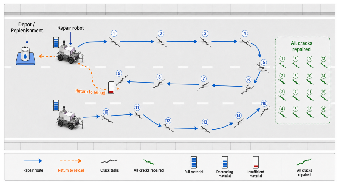
Figure 1 illustrates the operational logic. The blue arrows denote repair movement between crack tasks, while the orange dashed arrows denote replenishment returns under the following rule: The robot must replenish no later than the point at which the remaining sealant is insufficient for the next crack; during offline scheduling, an earlier capacity-feasible replenishment may be planned when it reduces the total operational objective. The schedule is complete only when every crack has been repaired and the robot has returned to the terminal depot.

The material consumption and service time of crack i are estimated from geometry:

$$q_i=\min \{q_{\max },\max \{q_{\min },\rho {\mathsf{\ell }}_i{w}_i{d}_i\}\},s_i={\displaystyle \frac{q_i}{r_f}},$$

(1)

where $\rho =3.6\times {10}^4\mathrm{L}/{\mathrm{m}}^3$, $q_{\min }=0.05\mathrm{L}$, $q_{\max }=1.35\mathrm{L}$, and $r_f$ is the filling rate. Because $q_i$ is proportional to ${\mathsf{\ell }}_i{w}_i{d}_i$ before clipping, uncertainty in surface geometry or in the assumed depth directly affects sealant demand and may change the location of replenishment boundaries. The present study therefore treats the volume model as a transparent baseline rather than a calibrated material-consumption law.

3.2. Priority Scores for Heuristics

An earlier draft considered an environmental/quality reward term $R_i$, but because every crack is mandatory in the reported SACRP setting, such a term would be constant across feasible schedules and would not change the exact optimum. We therefore remove it from the mandatory model and retain only the crack-priority score as a heuristic signal. The task priority $p_i$ is derived from the normalized crack length and width in the case-study preprocessing and is used only as a heuristic signal. Instead, the priority score is used in the construction heuristics and in the low-density removal operator described later. The latter is written directly in terms of $p_i$ to avoid confusing heuristic guidance with optimization reward:

$${\mathrm{\Delta }}_i^L={\displaystyle \frac{p_i}{s_i+{\tau }_{\mathrm{pre}\left(i\right),i}+{\tau }_{i,\mathrm{suc}\left(i\right)}+\omega q_i}},$$

(2)

where $\omega$ converts material demand into the same scale as time in this score, and cracks with small ${\mathrm{\Delta }}_i^L$ are removed first.

3.3. Compact MIP Model

Let $V=\{0,n+1\}\cup \mathcal{C}$ be the set of route nodes, where 0 is the starting depot and $n+1$ is the terminal depot. The fixed replenishment station is denoted by b; in the case-study instances, b is placed at the site entrance and is co-located with the depot. Let

$$\mathcal{A}=\left\{\right(i,j):i,j\in V,i\ne j,i\ne n+1,j\ne 0\}$$

(3)

be the admissible ordered arc set. For $(i,j)\in \mathcal{A}$, $d_{ij}$ is the direct distance from i to j, $d_{ib}$ is the return distance from i to the replenishment station, and $d_{bj}$ is the departure distance from the station to j. The corresponding travel times are

$${\tau }_{ij}={\displaystyle \frac{d_{ij}}{v}},{\tau }_{ibj}={\displaystyle \frac{d_{ib}+d_{bj}}{v}}.$$

(4)

We set $q_0=q_{n+1}=s_0=s_{n+1}=0$ and assume $q_i\le Q$ for every crack; otherwise, crack i must be split into multiple elementary repair tasks before scheduling. In the reported cases, the distance matrix is computed from anonymized local planar coordinates using Euclidean distance. The current study does not yet model lane-changing rules, obstacles, curb constraints, turning radii, or detailed robot kinematics. Incorporating road-network shortest paths and kinodynamic travel costs into $d_{ij}$ is therefore treated as future work rather than as a capability of the present case study.

The binary route variables are defined as follows:

$$x_{ij}=\left\{\begin{array}{cc}1,\hfill & \mathrm{if}\mathrm{the}\mathrm{robot}\mathrm{travels}\mathrm{directly}\mathrm{from}i\mathrm{to}j,\hfill \\ 0,\hfill & \mathrm{otherwise},\hfill \end{array}\right.$$

(5)

and

$$y_{ij}=\left\{\begin{array}{cc}1,\hfill & \mathrm{if}\mathrm{arc}i\to b\to j\mathrm{is}\mathrm{used}\mathrm{with}\mathrm{replenishment},\hfill \\ 0,\hfill & \mathrm{otherwise}.\hfill \end{array}\right.$$

(6)

Continuous variables $S_i$ and $M_i$ represent the service start time and remaining material after node i, respectively. The variable $u_i$ is an ordering variable used for subtour elimination. The following derived indicators are used in the objective and in the experimental reporting:

$$\begin{array}{cc}\hfill D(x,y)& =\sum _{(i,j)\in \mathcal{A}}{d}_{ij}{x}_{ij}+\sum _{(i,j)\in \mathcal{A}}(d_{ib}+d_{bj})y_{ij},\hfill \end{array}$$

(7)

$$\begin{array}{cc}\hfill D^b\left(y\right)& =\sum _{(i,j)\in \mathcal{A}}{d}_{ib}{y}_{ij},\hfill \end{array}$$

(8)

$$\begin{array}{cc}\hfill N^b\left(y\right)& =\sum _{(i,j)\in \mathcal{A}}{y}_{ij},\hfill \end{array}$$

(9)

$$\begin{array}{cc}\hfill T& =S_{n+1}.\hfill \end{array}$$

(10)

Here, D is total route distance, $D^b$ is the distance of return legs to the replenishment point, $N^b$ is the number of replenishment operations, and T is the operation makespan. The mandatory-operation version minimizes a weighted operational cost:

$$\begin{array}{cc}\hfill \min & Z={\alpha }_{D}D(x,y)+{\alpha }_B{D}^b\left(y\right)+{\alpha }_N{N}^b\left(y\right)+{\alpha }_{T}T,\hfill \end{array}$$

(11)

$$\begin{array}{cc}\hfill \mathrm{s}.\mathrm{t}.& \sum _{j:(0,j)\in \mathcal{A}}(x_{0j}+y_{0j})=1,\sum _{i:(i,n+1)\in \mathcal{A}}(x_{i,n+1}+y_{i,n+1})=1,\hfill \end{array}$$

(12)

$$\begin{array}{cc}\hfill & \sum _{j:(i,j)\in \mathcal{A}}(x_{ij}+y_{ij})=1,i\in \mathcal{C},\hfill \end{array}$$

(13)

$$\begin{array}{cc}\hfill & \sum _{j:(j,i)\in \mathcal{A}}(x_{ji}+y_{ji})=1,i\in \mathcal{C},\hfill \end{array}$$

(14)

$$\begin{array}{cc}\hfill & x_{ij}+y_{ij}\le 1,(i,j)\in \mathcal{A},\hfill \end{array}$$

(15)

$$\begin{array}{cc}\hfill & y_{0j}=0,(0,j)\in \mathcal{A},y_{i,n+1}=0,(i,n+1)\in \mathcal{A},\hfill \end{array}$$

(16)

$$\begin{array}{cc}\hfill & S_0=0,M_0=Q,\hfill \end{array}$$

(17)

$$\begin{array}{cc}\hfill & S_j\ge S_i+s_i+{\tau }_{ij}-M(1-x_{ij}),(i,j)\in \mathcal{A},\hfill \end{array}$$

(18)

$$\begin{array}{cc}\hfill & S_j\ge S_i+s_i+{\tau }_{ibj}+h_b-M(1-y_{ij}),(i,j)\in \mathcal{A},\hfill \end{array}$$

(19)

$$\begin{array}{cc}\hfill & M_j\le M_i-q_j+M(1-x_{ij}),(i,j)\in \mathcal{A},\hfill \end{array}$$

(20)

$$\begin{array}{cc}\hfill & M_j\ge M_i-q_j-M(1-x_{ij}),(i,j)\in \mathcal{A},\hfill \end{array}$$

(21)

$$\begin{array}{cc}\hfill & M_i\ge q_j-Q(1-x_{ij}),(i,j)\in \mathcal{A},j\in \mathcal{C},\hfill \end{array}$$

(22)

$$\begin{array}{cc}\hfill & M_j\le Q-q_j+M(1-y_{ij}),(i,j)\in \mathcal{A},\hfill \end{array}$$

(23)

$$\begin{array}{cc}\hfill & M_j\ge Q-q_j-M(1-y_{ij}),(i,j)\in \mathcal{A},\hfill \end{array}$$

(24)

$$\begin{array}{cc}\hfill & L_i\le S_i,S_i+s_i\le U_i,i\in \mathcal{C}(\mathrm{optional}\mathrm{closure}\mathrm{windows}),\hfill \end{array}$$

(25)

$$\begin{array}{cc}\hfill & u_i-u_j+n(x_{ij}+y_{ij})\le n-1,i,j\in \mathcal{C},i\ne j,\hfill \end{array}$$

(26)

$$\begin{array}{cc}\hfill & 1\le u_i\le n,0\le M_i\le Q,x_{ij},y_{ij}\in \{0,1\}.\hfill \end{array}$$

(27)

Objective (11) is the cost-minimization counterpart of the experimental objective. The coefficients $({\alpha }_D,{\alpha }_B,{\alpha }_N,{\alpha }_T)$ control the relative importance of total route distance, return-to-replenishment distance, replenishment frequency, and makespan. Constraints (12)–(14) enforce a single route that starts at the depot, visits every crack exactly once, and returns to the terminal depot. Constraint (15) prevents simultaneous direct and replenishment arcs between the same pair of nodes. Constraint (16) reflects the field rule that the robot starts with a full tank and does not count an artificial replenishment before the first task or immediately before the terminal return. Constraints (18) and (19) propagate time along direct and replenishment arcs. Constraints (20)–(22) enforce direct-arc material feasibility, while constraints (23) and (24) reset the tank after a replenishment arc. For example, if $Q=5.0$ L, $M_i=2.4$ L, and the next crack requires $q_j=2.8$ L, then a direct arc $x_{ij}=1$ is infeasible because constraint (22) requires $M_i\ge q_j$. A replenishment arc $y_{ij}=1$ is feasible and resets the material state to $M_j=Q-q_j=2.2$ L through constraints (23) and (24). Conversely, if $q_j=1.6$ L, a direct arc is feasible and constraints (20) and (21) give $M_j=0.8$ L. Constraint (25) is optional and is disabled in the case-study experiments because traffic-control time windows are not the dominant operational issue. Constraint (26) is the Miller–Tucker–Zemlin subtour-elimination condition [29].

Here, M is a sufficiently large constant used in the linearization; in the reported numerical experiments, $M={10}^6$, which is safely above every feasible time and material bound in the case study.

Theorem 1.

SACRP is NP-hard.

Proof. 

Consider the restricted case in which Q is sufficiently large to repair every crack without replenishment, all service times are zero, ${\alpha }_D=1$, ${\alpha }_B={\alpha }_N={\alpha }_T=0$, and the optional closure-window constraints are inactive. Objective (11) is then equivalent to finding a minimum-length tour through all crack nodes and the depot, which is the traveling salesman problem. Since the traveling salesman problem is NP-hard, SACRP is NP-hard.    □

The reduction establishes worst-case hardness. In practical SACRP instances, the replenishment constraints add a second coupling layer beyond TSP: a local change in crack order can move several downstream segment boundaries, alter the number of replenishment returns, and change both the direct-travel and return-to-station components of the objective. This is why the solution procedure below separates sequence search from exact replenishment segmentation instead of treating station visits as simple post-processing.

4. ALNS-DP Solution Method

4.1. Algorithmic Motivation

The SACRP solution method is designed around two field-driven observations. First, the robot is not allowed to skip cracks in the operation zone; therefore, the main decision is not task selection but the order in which mandatory cracks are repaired and the moments at which the robot returns to the replenishment point. Second, replenishment is a physical operation rather than a soft penalty. The robot must replenish no later than the point at which the remaining sealant is insufficient for the next crack; during offline scheduling, an earlier capacity-feasible replenishment may be planned when it reduces the total operational objective. A route plan is therefore useful only if it is both sequence-efficient and material-feasible.

A direct search over complete routes with explicit station visits is possible but inefficient. The same crack order can be represented by many different station-insertion patterns, many of which are dominated or infeasible because they either return too early, overload the tank, or create unnecessary back-and-forth movement. Conversely, a greedy rule that returns to the station only when the tank becomes empty is fast, but it may miss a better segmentation in which an earlier replenishment reduces later travel and improves the overall objective. These characteristics suggest that crack sequencing and replenishment segmentation should be separated rather than optimized by a single flat representation.

This motivates the ALNS-DP structure. The upper-level ALNS explores permutations of cracks, where large-neighborhood destroy-and-repair moves are effective for escaping poor spatial orders and rearranging clustered tasks. The lower-level DP decoder then computes the best replenishment-feasible segmentation for each candidate permutation. In this way, every candidate repaired sequence remains complete, replenishment feasibility is handled exactly for the fixed sequence, and the stochastic search effort is concentrated on the combinatorial structure that most affects travel distance and makespan. The problem-specific operators introduced later are built to exploit this same logic: they remove cracks that create travel pressure, replenishment pressure, or low-density detours, and then reinsert them using distance-, regret-, and refill-aware scores.

4.2. Encoding and Decoding

ALNS-DP uses an indirect representation. The upper-level solution is encoded as a permutation

$$\pi =({\pi }_1,{\pi }_2,\dots ,{\pi }_n),\{{\pi }_1,\dots ,{\pi }_n\}=\mathcal{C},{\pi }_a\ne {\pi }_j(a\ne j),$$

(28)

where ${\pi }_t$ is the tth crack to be considered for repair. The permutation contains no explicit replenishment decision. Replenishment decisions are produced by a decoder that inserts station visits into the sequence.

Let $\sigma =({\sigma }_0,{\sigma }_1,\cdots ,{\sigma }_m)$ be a segmentation vector with

$$0={\sigma }_0<{\sigma }_1<\dots <{\sigma }_m=n.$$

(29)

Segment g contains cracks ${\pi }_{{\sigma }_{g-1}+1},\dots ,{\pi }_{{\sigma }_g}$ and must satisfy the material-capacity condition

$$Q_g(\pi ,\sigma )={\displaystyle \sum _{t={\sigma }_{g-1}+1}^{{\sigma }_g}}{q}_{{\pi }_t}\le Q,g=1,\dots ,m.$$

(30)

Define the within-segment path

$${\mathcal{S}}_g={\pi }_{{\sigma }_{g-1}+1}\to {\pi }_{{\sigma }_{g-1}+2}\to \cdots \to {\pi }_{{\sigma }_g}.$$

(31)

The decoded route is therefore

$$\mathcal{R}(\pi ,\sigma )=0\to {\mathcal{S}}_1\to b\to {\mathcal{S}}_2\to b\to \cdots \to b\to {\mathcal{S}}_m\to n+1.$$

(32)

Only the boundaries ${\sigma }_1,\dots ,{\sigma }_{m-1}$ are replenishment returns; all cracks remain in the schedule. The remaining material after repairing the tth crack in segment g is

$$M_{{\pi }_t}=Q-{\displaystyle \sum _{r={\sigma }_{g-1}+1}^t}{q}_{{\pi }_r},{\sigma }_{g-1}<t\le {\sigma }_g.$$

(33)

Thus, encoding changes the repair order, while decoding converts that order into an executable operation plan with explicit replenishment trips, timestamps, and material inventory.

4.3. Dynamic-Programming Decoder

For a fixed permutation $\pi$, the decoder chooses the best segmentation $\sigma$. Define the cumulative segment demand, internal route distance, and service time as

$$\begin{array}{cc}\hfill Q(a,j)& ={\displaystyle \sum _{t=a}^j}{q}_{{\pi }_t},\hfill \end{array}$$

(34)

$$\begin{array}{cc}\hfill I(a,j)& ={\displaystyle \sum _{t=a}^{j-1}}{d}_{{\pi }_t,{\pi }_{t+1}},\hfill \end{array}$$

(35)

$$\begin{array}{cc}\hfill S(a,j)& ={\displaystyle \sum _{t=a}^j}{s}_{{\pi }_t},\hfill \end{array}$$

(36)

where $1\le a\le j\le n$ and $I(a,a)=0$. Let $o_h=0$ if $h=0$ and $o_h=b$ if $h>0$. If cracks ${\pi }_{h+1},\dots ,{\pi }_j$ form a non-final segment, the robot starts from $o_h$, repairs the segment, returns to the replenishment point, and reloads. Its segment cost is

$$\begin{array}{cc}\hfill {\mathcal{C}}^B(h,j)=& {\alpha }_D\left(d_{o_h,{\pi }_{h+1}}+I(h+1,j)+d_{{\pi }_j,b}\right)\hfill \\ \hfill & +{\alpha }_B{d}_{{\pi }_j,b}+{\alpha }_N+{\alpha }_T\left({\displaystyle \frac{d_{o_h,{\pi }_{h+1}}+I(h+1,j)+d_{{\pi }_j,b}}{v}}+S(h+1,j)+h_b\right).\hfill \end{array}$$

(37)

If ${\pi }_{h+1},\dots ,{\pi }_n$ is the final segment, the robot returns to the terminal depot and no replenishment is counted after completion:

$$\begin{array}{cc}\hfill {\mathcal{C}}^T(h,n)=& {\alpha }_D\left(d_{o_h,{\pi }_{h+1}}+I(h+1,n)+d_{{\pi }_n,n+1}\right)\hfill \\ \hfill & +{\alpha }_T\left({\displaystyle \frac{d_{o_h,{\pi }_{h+1}}+I(h+1,n)+d_{{\pi }_n,n+1}}{v}}+S(h+1,n)\right).\hfill \end{array}$$

(38)

The DP state $G\left(j\right)$ is the minimum cost required to repair the prefix ${\pi }_1,\dots ,{\pi }_j$ and be ready at the replenishment station with a full tank. The recurrence is

$$\begin{array}{cc}\hfill G\left(0\right)& =0,\hfill \end{array}$$

(39)

$$\begin{array}{cc}\hfill G\left(j\right)& =\underset{\begin{array}{c}0\le h<j\\ Q(h+1,j)\le Q\end{array}}{\min }\left\{G\left(h\right)+{\mathcal{C}}^B(h,j)\right\},j=1,\dots ,n-1.\hfill \end{array}$$

(40)

The decoded objective value of the complete sequence is

$$\mathrm{\Phi }\left(\pi \right)=\underset{\begin{array}{c}0\le h<n\\ Q(h+1,n)\le Q\end{array}}{\min }\left\{G\left(h\right)+{\mathcal{C}}^T(h,n)\right\}.$$

(41)

The minimizing predecessor of each state is stored, and backtracking from Equation (41) yields $\sigma$. This decoder is also used after every destroy-and-repair move, so infeasible candidate sequences do not need separate penalty handling as long as $q_i\le Q$ for all elementary tasks.

Proposition 1.

For any fixed crack sequence π of length n, the optimal replenishment segmentation under Equations (40) and (41) can be found in $O\left(n^2\right)$ time.

Proof. 

Any feasible replenishment plan for a fixed permutation is a partition of the ordered sequence into consecutive capacity-feasible segments. For each prefix ending at j, Equation (40) enumerates the start of the last non-final segment and combines it with the optimal decoded cost of the previous prefix. Equation (41) performs the same enumeration for the final segment. By induction on j, $G\left(j\right)$ is optimal for every prefix, and the final enumeration is optimal for the full sequence. There are $O\left(n^2\right)$ candidate segments, and $Q(a,j)$, $I(a,j)$, and $S(a,j)$ can be obtained from cumulative arrays, so each segment can be evaluated in $O\left(1\right)$ time after preprocessing.    □

When embedded in ALNS, this decoder is called for each candidate sequence and for sampled insertion evaluations. Proposition 1 concerns one exact decoding pass for a fixed crack sequence, whereas the bottleneck discussed here comes from repeating that exact pass many times inside the metaheuristic. If at most $s_{\mathrm{ins}}$ insertion positions are evaluated for each removed crack and $m_r$ cracks are removed, one repair phase requires $O\left(m_r{s}_{\mathrm{ins}}{n}^2\right)$ decoding work in the worst case. This is why the decoder is the main scalability bottleneck for very large crack sets; Section 5 therefore reports a separate decoding-time test up to 500 cracks and discusses incremental or approximate segmentation as future acceleration options. Algorithm 1 summarizes this decoder.

Algorithm 1 DP decoder for a fixed crack sequence.

Require: Crack sequence $\pi$, demand $q_i$, service time $s_i$, distance matrix d, capacity Q Ensure: Objective $\mathrm{\Phi }\left(\pi \right)$, segmentation $\sigma$, event list $\mathcal{E}$     Precompute $Q(a,j)$, $I(a,j)$, and $S(a,j)$ for all $1\le a\le j\le n$     Set $G\left(0\right)\leftarrow 0$ and $\mathrm{pred}\left(0\right)\leftarrow -1$     for  $j=1,\dots ,n-1$  do           $G\left(j\right)\leftarrow +\infty$, $\mathrm{pred}\left(j\right)\leftarrow -1$           for $h=0,\dots ,j-1$ do                 if $Q(h+1,j)\le Q$ then                      $c\leftarrow G\left(h\right)+{\mathcal{C}}^B(h,j)$                      if $c<G\left(j\right)$ then                            $G\left(j\right)\leftarrow c$, $\mathrm{pred}\left(j\right)\leftarrow h$                      end if                 end if           end for     end for     $\mathrm{\Phi }\left(\pi \right)\leftarrow +\infty$, $h^{★}\leftarrow -1$     for  $h=0,\dots ,n-1$  do           if $Q(h+1,n)\le Q$ then                 $c\leftarrow G\left(h\right)+{\mathcal{C}}^T(h,n)$                 if $c<\mathrm{\Phi }\left(\pi \right)$ then                      $\mathrm{\Phi }\left(\pi \right)\leftarrow c$, $h^{★}\leftarrow h$                 end if           end if     end for     Backtrack from $h^{★}$ through $\mathrm{pred}(·)$ to obtain $\sigma$     Generate travel, repair, and refill events from $\mathcal{R}(\pi ,\sigma )$     Compute timestamps and material inventory using Equation (33)     return $\mathrm{\Phi }\left(\pi \right)$, $\sigma$, $\mathcal{E}$

4.4. Adaptive Large-Neighborhood Search

The upper-level ALNS searches over the permutation $\pi$. Destroy operators remove a subset of cracks from the incumbent sequence, and repair operators reinsert every removed crack. The candidate sequence is then decoded by the DP module. Let ${\pi }^c$ be the incumbent sequence and ${\pi }^{\prime }$ be a candidate. The move cost is

$$\mathrm{\Delta }=\mathrm{\Phi }\left({\pi }^{\prime }\right)-\mathrm{\Phi }\left({\pi }^c\right).$$

(42)

The candidate is always accepted if $\mathrm{\Delta }\le 0$; otherwise, it is accepted with simulated-annealing probability

$$P_{\mathrm{acc}}({\pi }^{\prime },{\pi }^c)=\exp \left(-{\displaystyle \frac{\mathrm{\Delta }}{{\mathrm{\Theta }}_r}}\right),{\mathrm{\Theta }}_{r+1}=\eta {\mathrm{\Theta }}_r,0<\eta <1,$$

(43)

where ${\mathrm{\Theta }}_r$ is the temperature at iteration r.

Operator selection follows adaptive roulette weights. If $\mathrm{\Omega }$ is the operator set and $w_o$ is the current weight of operator o, the selection probability is

$$\mathrm{Pr}\left(o\right)={\displaystyle \frac{w_o}{{\sum }_{k\in \mathrm{\Omega }}{w}_k}}.$$

(44)

At the end of each update segment, the weight is smoothed by

$$w_o\leftarrow (1-\theta )w_o+\theta {\displaystyle \frac{{\psi }_o}{\max (1,{\nu }_o)}},$$

(45)

where ${\psi }_o$ is the accumulated score and ${\nu }_o$ is the number of times operator o was used. The score is increased when an operator produces a new global best solution, improves the incumbent, or generates an accepted non-improving solution. The numerical settings used for ALNS-DP are listed in

Table 3. Numerical parameters used for ALNS-DP in the revised experiments.

Parameter	Symbol	Value
Main iteration limit	$R_{\max }$	170
Initial temperature	${\mathrm{\Theta }}_1$	8.0
Cooling factor	$\eta$	0.996
Operator-update interval	L	20 iterations
Removal-size bound	$m_r$	2 to 8 nodes for ALNS-DP, with default target $\lfloor 0.09n\rfloor$
Operator reward scores	$({\rho }_1,{\rho }_2,{\rho }_3)$	(12, 6, 2)
Weight smoothing coefficient	$\theta$	0.20
Low-density demand weight	$\omega$	$1.0\min /\mathrm{L}$
Refill-aware insertion penalty	$\zeta$	1000 objective units/L
Regret insertion order	k	2
Insertion-position sampling	–	all positions if $n\le 24$; otherwise endpoints plus up to 8 sampled positions
Local-search probability	$p_{\mathrm{LS}}$	0.45
Local-search interval	$L_{\mathrm{LS}}$	10 iterations
Local-search range	–	relocate over sampled insertion positions; one bounded 2-opt reversal per triggered iteration
Stopping criterion	–	fixed $R_{\max }$ or completion of all insertions
Random-seed policy	–	for case c and run $r=1,\dots ,10$, ALNS0 uses $3101+97c+1009r$ and ALNS-DP uses $4101+131c+1009r$
CPU	–	12th Gen Intel(R) Core(TM) i7-12700H, 14 cores and 20 logical processors
RAM	–	31.7 GB
Operating system	–	Microsoft Windows 11, version 10.0.26200
Python and packages	–	Python 3.10.9; NumPy 2.2.6; SciPy 1.15.3; PuLP 3.3.1; Matplotlib 3.10.8
MIP solver	–	CBC 2.10.3 through PuLP PULP_CBC_CMD
${\kappa }_d$	–	0.52, engineering depth ratio used in the case study
$\rho$	–	$3.6\times {10}^4\mathrm{L}/{\mathrm{m}}^3$, volume-to-sealant conversion
M	–	${10}^6$, Big-M constant used in the compact MIP

. Algorithm 2 summarizes the complete ALNS-DP procedure.

Algorithm 2  ALNS-DP for SACRP.

Require: Crack set $\mathcal{C}$, parameters $(Q,v,h_b)$, iteration limit $R_{\max }$, segment length L Ensure: Best sequence ${\pi }^{best}$, segmentation ${\sigma }^{best}$, and decoded operation schedule     Build initial pool ${\mathcal{P}}_0$ using NNG, PFG, SWP, RAG, and reward-density insertion     for all  $\pi \in {\mathcal{P}}_0$  do           $\left(\mathrm{\Phi }\right(\pi ),\sigma ,\mathcal{E})\leftarrow$ DecodeDP(π) using Algorithm 1     end for     ${\pi }^c\leftarrow \arg {\min }_{\pi \in {\mathcal{P}}_0}\mathrm{\Phi }\left(\pi \right)$, ${\pi }^{best}\leftarrow {\pi }^c$     Initialize weights $w_o\leftarrow 1$, scores ${\psi }_o\leftarrow 0$, and counts ${\nu }_o\leftarrow 0$     Initialize temperature ${\mathrm{\Theta }}_1$, cooling factor $\eta$, and reward scores ${\rho }_1>{\rho }_2>{\rho }_3>0$     for  $r=1,\dots ,R_{\max }$  do           Select destroy operator d and repair operator a using Equation (44)           Draw removal size $m_r\in [\lceil {\nu }_{\min }n\rceil ,\lceil {\nu }_{\max }n\rceil ]$           $({\pi }^{-},\mathcal{B})\leftarrow$ Destroy(πc, d, mr)           while $\mathcal{B}\ne ⌀$ do                 for all $i\in \mathcal{B}$ do                        Evaluate sampled insertion positions by Equation (49)                        Compute greedy, regret, or refill-aware score according to operator a                 end for                 Select $(i^{★},p^{★})$ with the best repair score                 π− ← Insert$({\pi }^{-},i^{★},p^{★})$, $\mathcal{B}\leftarrow \mathcal{B}\setminus \left\{i^{★}\right\}$           end while           ${\pi }^{\prime }\leftarrow {\pi }^{-}$           if $r\mathrm{mod}{L}_{\mathrm{LS}}=0$ or $\mathrm{rand}(0,1)<p_{\mathrm{LS}}$ then                 Apply bounded relocate and 2-opt moves accepted by the DP decoder           end if           $(\mathrm{\Phi }\left({\pi }^{\prime }\right),{\sigma }^{\prime },{\mathcal{E}}^{\prime })\leftarrow$ DecodeDP(π′)           $\mathrm{\Delta }\leftarrow \mathrm{\Phi }\left({\pi }^{\prime }\right)-\mathrm{\Phi }\left({\pi }^c\right)$           $\mathrm{accept}\leftarrow (\mathrm{\Delta }\le 0)$ or $\left(\mathrm{rand}(0,1)<\exp (-\mathrm{\Delta }/{\mathrm{\Theta }}_r)\right)$           if $\mathrm{\Phi }\left({\pi }^{\prime }\right)<\mathrm{\Phi }\left({\pi }^{best}\right)$ then                 ${\pi }^{best}\leftarrow {\pi }^{\prime }$, ${\sigma }^{best}\leftarrow {\sigma }^{\prime }$, ${\psi }_d,{\psi }_a\leftarrow {\psi }_d+{\rho }_1,{\psi }_a+{\rho }_1$           else if $\mathrm{\Delta }<0$ then                 ${\psi }_d,{\psi }_a\leftarrow {\psi }_d+{\rho }_2,{\psi }_a+{\rho }_2$           else if accept then                 ${\psi }_d,{\psi }_a\leftarrow {\psi }_d+{\rho }_3,{\psi }_a+{\rho }_3$           end if           if accept then                 ${\pi }^c\leftarrow {\pi }^{\prime }$           end if           ${\nu }_d,{\nu }_a\leftarrow {\nu }_d+1,{\nu }_a+1$ and ${\mathrm{\Theta }}_{r+1}\leftarrow \eta {\mathrm{\Theta }}_r$           if $r\mathrm{mod}L=0$ then                 for all o in the destroy and repair operator sets do                        Update $w_o$ using Equation (45); reset ${\psi }_o,{\nu }_o\leftarrow 0$                 end for           end if     end for     $(\mathrm{\Phi }\left({\pi }^{best}\right),{\sigma }^{best},{\mathcal{E}}^{best})\leftarrow$ DecodeDP(πbest)     return ${\pi }^{best}$, ${\sigma }^{best}$, and ${\mathcal{E}}^{best}$

4.5. Problem-Specific Operators

Let $\mathrm{pre}\left(i\right)$ and $\mathrm{suc}\left(i\right)$ be the predecessor and successor of crack i in the current permutation. A travel-pressure score is computed as

$${\mathrm{\Delta }}_i^D=d_{\mathrm{pre}\left(i\right),i}+d_{i,\mathrm{suc}\left(i\right)}-d_{\mathrm{pre}\left(i\right),\mathrm{suc}\left(i\right)}.$$

(46)

Cracks with large ${\mathrm{\Delta }}_i^D$ are likely to be costly detours and are removed with high probability. A replenishment-pressure score uses the decoded material balance:

$${\mathrm{\Delta }}_i^Q={\displaystyle \frac{q_i}{M_i^{-}+ϵ}}\mathbf{1}\{M_i^{-}<\overline{q}\},$$

(47)

where $M_i^{-}$ is the material available immediately before crack i, $\overline{q}$ is the mean crack demand, and $ϵ$ avoids division by zero. This operator focuses on cracks near segment boundaries where a small demand change can trigger an additional return to the replenishment point. A low-density score is

$${\mathrm{\Delta }}_i^L={\displaystyle \frac{p_i}{s_i+{\tau }_{\mathrm{pre}\left(i\right),i}+{\tau }_{i,\mathrm{suc}\left(i\right)}+\omega q_i}},$$

(48)

where $\omega$ converts material demand into the same scale as time in this density score, and cracks with small ${\mathrm{\Delta }}_i^L$ are removed first.

During repair, the insertion cost of removed crack i at position p is evaluated by the decoded objective:

$${\delta }_{i,p}=\mathrm{\Phi }\left(\mathrm{Insert}(\pi ,i,p)\right)-\mathrm{\Phi }\left(\pi \right).$$

(49)

Greedy insertion selects the pair $(i,p)$ with minimum ${\delta }_{i,p}$. Regret-k insertion first sorts all feasible insertion positions of crack i so that ${\delta }_{i,\left(1\right)}\le {\delta }_{i,\left(2\right)}\le \dots$, and then selects the crack with the largest regret value

$${\mathrm{Regret}}_k\left(i\right)={\displaystyle \sum _{r=2}^k}\left({\delta }_{i,\left(r\right)}-{\delta }_{i,\left(1\right)}\right).$$

(50)

The selected crack is inserted at its best position $\left(1\right)$. A refill-aware insertion variant adds a boundary penalty,

$${\tilde{\delta }}_{i,p}={\delta }_{i,p}+\zeta \max \{0,Q(a,p)+q_i-Q\},$$

(51)

where $Q(a,p)$ is the demand of the segment into which crack i would be inserted. This discourages insertions that create unnecessary replenishment returns unless they also produce enough travel savings.

5. Real Case Study

5.1. Case Description and Data Processing

The case study is based on real pavement-maintenance operations at Anhui Construction Engineering Sanjian in Hefei, Anhui Province, China. The raw site coordinates were transformed into local operation-zone coordinate systems with the depot and replenishment point placed at the site entrance. Twelve operation-zone cases are constructed from the field records. The original crack-level records used to construct these cases are provided in the Supplementary Materials (File S1). Each case must be fully completed: all detected cracks are scheduled. The robot must replenish no later than the point at which the remaining sealant is insufficient for the next crack; during offline scheduling, an earlier capacity-feasible replenishment may be planned when it reduces the total operational objective. The base layout follows the field record in which the supply point was located at the work-zone entrance. Because practical projects may place supply at the center, the far end, or multiple temporary locations, Section 5 adds a replenishment-location sensitivity test. The 12 zones come from a single field source; thus, the results should be interpreted as a realistic single-source validation rather than as a universal pavement-network benchmark.

The crack priority $p_i$ is derived from the field severity attributes rather than set uniformly. Specifically, crack length and width are min–max normalized within each operation zone, and the priority score is computed as

$$p_i=1+4\left(0.45{\overline{\mathsf{\ell }}}_i+0.55{\overline{w}}_i\right),$$

(52)

where ${\overline{\mathsf{\ell }}}_i$ and ${\overline{w}}_i$ are normalized length and width. This maps each crack to a reproducible priority range of 1–5 and gives slightly higher weight to crack width because wider cracks typically require more urgent sealing and consume more material. Depth is retained in the task table for demand estimation, but it is an engineering estimate rather than a direct robot-measured attribute in the current case study. It is not used in the priority score because the routine inspection records provide surface length and width more consistently than depth. The default case-study parameters are listed in

Table 4. Default parameters for the case-study operation cases.

Parameter	Symbol	Value
Case location	–	Hefei, Anhui Province, China
Company	–	Anhui Construction Engineering Sanjian
Number of operation cases	–	12
Cracks per case	n	18–64
Robot speed	v	$30\mathrm{m}/\min$
Filling rate	$r_f$	$1.20\mathrm{L}/\min$
Material capacity	Q	$5\mathrm{L}$
Replenishment time	$h_b$	$5\min$
Priority range	$p_i$	1–5 from Equation (52)
Completion rule	–	All cracks repaired
Return rule	–	The robot must replenish no later than the point at which the remaining sealant is insufficient for the next crack; during offline scheduling, an earlier capacity-feasible replenishment may be planned when it reduces the total operational objective.

.

5.2. Evaluation Indicators

To make the field operations interpretable, the evaluation emphasizes replenishment-related indicators rather than a hard time-window constraint. The main indicators are final objective value, route distance, makespan, travel time, repair time, replenishment time, number of replenishments, replenishment-related distance, sealant use, material utilization, and computation time. The makespan is reported as the total work duration required to finish an operation zone, not as a strict feasibility filter.

The material utilization of a schedule is reported as

$$U={\displaystyle \frac{{\sum }_{i\in \mathcal{C}}{q}_i}{Q(N^b+1)}}\times 100\%,$$

(53)

where $N^b$ is the number of replenishments and the denominator counts the initial tank and each refill. In the demand-error replay experiments, an emergency replenishment cost is accumulated whenever the nominal plan becomes materially infeasible:

$$C_{\mathrm{emg}}=\sum _{e\in {\mathcal{E}}_{\mathrm{emg}}}\left({\alpha }_D\mathrm{\Delta }{D}_e+{\alpha }_B{d}_{i_{e}b}+{\alpha }_N+{\alpha }_T\left({\displaystyle \frac{\mathrm{\Delta }{D}_e}{v}}+h_b\right)\right),$$

(54)

where $\mathrm{\Delta }{D}_e$ is the extra distance created by the emergency detour to the replenishment point for event e.

For the computational comparison, the final objective is

$$F=D+0.35D^b+18N^b+5T,$$

(55)

where D is the total route distance, $D^b$ is the distance associated with return-to-replenishment legs, $N^b$ is the number of replenishments, and T is the makespan. The coefficients define a normalized operational scoring index for algorithm comparison, not a calibrated economic cost function. Route distance is retained as the base term, while return-to-replenishment distance, replenishment count, and makespan are added to reflect repeated backtracking, docking/restart operations, and total work duration. Because project-specific calibration data for traffic-control cost, labor cost, and docking overhead are not available in the current field records, these values are treated as planning weights; the stability of algorithm rankings under alternative weights is tested below. Because all cracks are mandatory in the case-study operation cases, the objective evaluates how efficiently the same complete repair task is executed.

The baselines are nearest-neighbor greedy (NNG), priority-first greedy (PFG), longitudinal sweep (SWP), refill-aware greedy (RAG), and a generic ALNS without the proposed problem-specific destroy and repair logic (ALNS₀). The proposed ALNS-DP uses the same route representation but adds replenishment-pressure, spatial-cluster, insertion-cost-aware search operators, and DP-based replenishment decoding. Each algorithm is run ten times on every case. Deterministic heuristics are repeated under the same settings to record comparable CPU statistics, while ALNS₀ and ALNS-DP use independent random seeds.

5.3. Multi-Indicator Comparison

Table 5. Final objective comparison over 12 operation cases. Values are mean (standard deviation) over ten runs, and the rightmost column reports the case-wise reduction in ALNS-DP relative to ALNS₀.

Case	NNG	PFG	SWP	RAG	ALNS0	ALNS-DP	Red.
Case-01	2427.2 (0.0)	3245.4 (0.0)	2427.2 (0.0)	2424.2 (0.0)	2423.5 (1.4)	2413.8 (3.0)	0.40%
Case-02	4298.0 (0.0)	5457.5 (0.0)	4298.0 (0.0)	3859.8 (0.0)	3760.8 (51.9)	3556.5 (53.5)	5.43%
Case-03	5238.9 (0.0)	6443.4 (0.0)	5303.1 (0.0)	4880.8 (0.0)	4748.0 (148.9)	4343.6 (48.8)	8.52%
Case-04	6739.1 (0.0)	9022.6 (0.0)	6739.1 (0.0)	7208.1 (0.0)	6716.7 (21.2)	6476.3 (30.5)	3.58%
Case-05	8018.5 (0.0)	12,142.7 (0.0)	8018.5 (0.0)	9288.4 (0.0)	7919.8 (100.4)	7319.4 (19.2)	7.58%
Case-06	10,176.9 (0.0)	16,367.2 (0.0)	10,176.9 (0.0)	10,762.8 (0.0)	10,175.8 (3.5)	9905.9 (63.6)	2.65%
Case-07	12,904.1 (0.0)	18,828.4 (0.0)	12,904.1 (0.0)	13,924.8 (0.0)	12,904.1 (0.0)	12,497.2 (39.8)	3.15%
Case-08	14,872.4 (0.0)	20,362.1 (0.0)	14,872.4 (0.0)	17,650.0 (0.0)	14,791.8 (89.3)	13,777.8 (49.4)	6.86%
Case-09	16,456.6 (0.0)	27,630.9 (0.0)	16,456.6 (0.0)	18,472.9 (0.0)	16,233.9 (234.2)	15,170.2 (61.1)	6.55%
Case-10	19,285.1 (0.0)	30,122.5 (0.0)	19,285.1 (0.0)	22,499.8 (0.0)	19,228.7 (178.3)	18,290.8 (200.5)	4.88%
Case-11	22,106.8 (0.0)	33,123.6 (0.0)	22,106.8 (0.0)	23,914.1 (0.0)	21,956.0 (205.7)	20,212.0 (241.8)	7.94%
Case-12	28,244.7 (0.0)	39,061.3 (0.0)	28,309.5 (0.0)	30,117.3 (0.0)	28,244.7 (0.0)	27,189.4 (219.9)	3.74%
Mean reduction vs. ALNS0							5.11%
Reduction range							0.40–8.52%

and

Table 6. CPU time in seconds over ten runs for every case and algorithm. Values are mean (standard deviation).

Case	NNG	PFG	SWP	RAG	ALNS0	ALNS-DP
Case-01	0.000 (0.000)	0.000 (0.000)	0.000 (0.000)	0.000 (0.000)	0.012 (0.004)	1.513 (0.258)
Case-02	0.000 (0.000)	0.000 (0.000)	0.000 (0.000)	0.000 (0.000)	0.011 (0.003)	1.920 (0.481)
Case-03	0.000 (0.000)	0.000 (0.000)	0.000 (0.000)	0.000 (0.000)	0.014 (0.005)	1.838 (0.331)
Case-04	0.000 (0.000)	0.000 (0.000)	0.000 (0.000)	0.000 (0.000)	0.017 (0.009)	1.170 (0.233)
Case-05	0.000 (0.000)	0.000 (0.000)	0.000 (0.000)	0.000 (0.000)	0.016 (0.005)	1.715 (0.252)
Case-06	0.000 (0.000)	0.000 (0.000)	0.000 (0.000)	0.000 (0.000)	0.016 (0.001)	1.938 (0.292)
Case-07	0.000 (0.000)	0.000 (0.000)	0.000 (0.000)	0.000 (0.000)	0.022 (0.008)	2.666 (0.452)
Case-08	0.000 (0.000)	0.000 (0.000)	0.000 (0.000)	0.001 (0.000)	0.030 (0.010)	4.336 (1.445)
Case-09	0.001 (0.000)	0.000 (0.000)	0.000 (0.000)	0.001 (0.000)	0.030 (0.013)	4.523 (1.919)
Case-10	0.001 (0.000)	0.000 (0.000)	0.000 (0.000)	0.001 (0.000)	0.027 (0.007)	4.468 (0.538)
Case-11	0.001 (0.001)	0.000 (0.000)	0.000 (0.000)	0.002 (0.001)	0.056 (0.023)	11.461 (3.651)
Case-12	0.001 (0.000)	0.000 (0.000)	0.000 (0.000)	0.001 (0.000)	0.029 (0.004)	6.885 (0.962)

report all 12 cases and all six algorithms. Values in Table 5 are mean final objective values with standard deviations over ten runs; bold text marks the best mean objective in each case. ALNS-DP obtains the best mean objective for all 12 cases, showing that its advantage is not produced by omitting difficult cracks. Every algorithm repairs every crack, and the difference is caused by the route order and the timing of returns to the replenishment point. The summary rows in Table 5 make the headline objective numbers explicit: a 5.11% mean reduction and a 0.40–8.52% range. The rightmost column in Table 5 reports the case-wise reduction in ALNS-DP relative to ALNS₀, and the footer rows summarize the mean reduction and range.

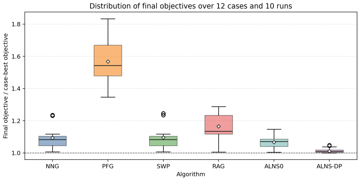
Figure 2 shows the distribution of normalized final objective values over the 120 observations of each algorithm. The normalization uses the best objective found for each case as the denominator, so the boxplot compares algorithm stability without letting larger work zones dominate the visual scale. The high median of PFG indicates that repairing high-priority cracks first without considering spatial continuity and replenishment position creates long cross-zone movements.

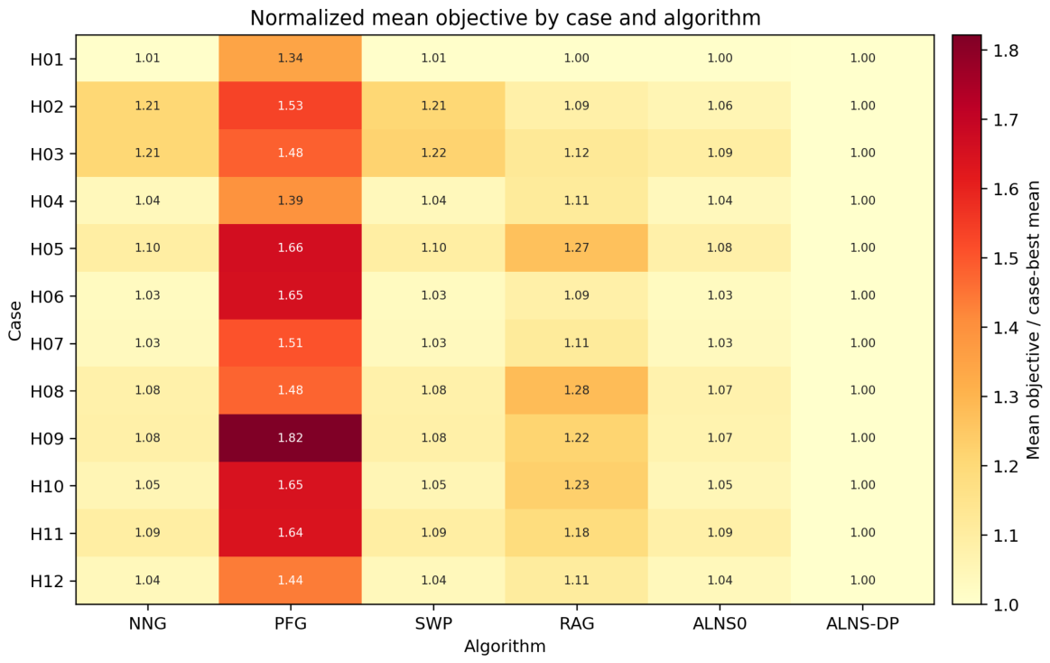
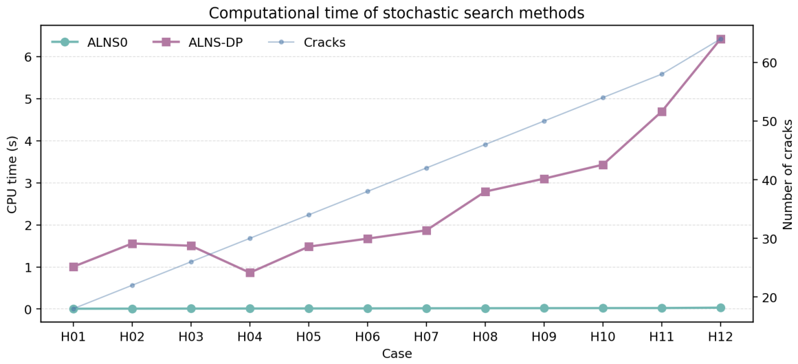
Figure 3 further reports the case-by-algorithm normalized mean objective values. This heatmap makes the cross-case pattern explicit: ALNS-DP is consistently closest to the case-best value, whereas PFG deteriorates sharply on longer and denser operation zones. Figure 4 gives the corresponding computational profile of the stochastic search methods. The CPU cost of ALNS-DP increases with case size because each sequence evaluation uses the replenishment-aware DP decoder, but the absolute time remains suitable for pre-operation planning.

5.4. Statistical, Ablation, and Sensitivity Analysis

To assess proximity to the optimum, three small instances were extracted from representative operation zones and solved with an exact set-partitioning MIP that is equivalent to the compact formulation under the depot–station layout used in the case study.

Table 7. Small exact MIP benchmark for ALNS-DP, including exact runtime and ten-run mean gap.

Case	Cracks	MIP Status	Exact Obj.	Exact Time	ALNS-DP Best	Mean Gap
Case-03	8	Optimal	1259.30	0.088 s	1259.30	0.000%
Case-08	10	Optimal	2665.67	0.082 s	2665.67	0.000%
Case-12	12	Optimal	5484.08	0.080 s	5484.08	0.000%

shows that ALNS-DP reached the exact optimum in all three tests.

Because the exact benchmark solutions in Table 7 are connected and contain no disconnected subtours, they also provide an empirical check that Equation (26) eliminates subtours in the reported depot–station layout.

The statistical analysis was also strengthened. Because six algorithms are compared over the same 12 cases, a Friedman test was first applied to the case-level normalized mean objectives. The overall difference among algorithms is significant (${\chi }^2=54.914$, $p=1.36\times {10}^{-10}$). Post hoc one-sided Wilcoxon signed-rank tests comparing ALNS-DP with each alternative remain significant after Bonferroni correction; the adjusted p-value is 0.00122 for each comparison. The one-sided tests follow the pre-specified directional hypothesis that ALNS-DP should reduce the operational objective relative to the baselines. For the strongest stochastic baseline ALNS₀, the Wilcoxon statistic is 0.000 with $p=0.000244$, the rank-biserial effect size is 1.000, and a bootstrap 95% confidence interval for the mean normalized objective reduction is [0.040, 0.069]. The operation zone is treated as the independent experimental unit; the ten runs within each zone quantify algorithmic randomness and are summarized before case-level inference. Because only 12 case-level observations are available, these results are interpreted as strong evidence for this case set rather than as a population-level guarantee.

Table 8. All-case ablation screening over the 12 operation zones. Normalized objective is relative to the full ALNS-DP variant.

Variant	Norm. Obj.	Change	CPU (s)
ALNS-DP full	1.000	+0.00%	0.727
w/o DP decoder	1.021	+2.06%	0.242
w/o specific operators	1.017	+1.72%	0.019
w/o replenishment-pressure removal	1.003	+0.29%	0.727

reports an all-case ablation screening over the 12 operation zones. Replacing the DP decoder with greedy replenishment increases the normalized objective by 2.06%, removing the problem-specific operator set increases it by 1.72%, and removing only the replenishment-pressure removal operator has a smaller effect of 0.29%. The result indicates that the main contribution comes from the DP segmentation and the full problem-specific search design.

Table 9. Objective-weight sensitivity over the 12 cases.

Scenario	${\mathit{\alpha }}_{\mathit{D}}$	${\mathit{\alpha }}_{\mathit{B}}$	${\mathit{\alpha }}_{\mathit{N}}$	${\mathit{\alpha }}_{\mathit{T}}$	Mean Ratio	Wins
Baseline	1.00	0.35	18.0	5.0	1.000	12/12
Higher return-distance penalty	1.00	0.50	18.0	5.0	1.000	12/12
Lower refill penalty	1.00	0.35	9.0	5.0	1.000	12/12
Higher refill penalty	1.00	0.35	27.0	5.0	1.000	12/12
Higher makespan penalty	1.00	0.35	18.0	7.0	1.000	12/12

examines the objective-weight settings. The tested scenarios increase the penalty on return-to-replenishment distance, decrease and increase the fixed replenishment penalty, and increase the makespan coefficient. The table reports the exact coefficients used in each scenario. ALNS-DP remains the best method in all 12 cases under every scenario, so the algorithm ranking is not an artifact of one narrow coefficient setting.

Replenishment-location sensitivity was evaluated on Case-03, Case-08, and Case-12 by moving the supply point from the entrance to the center or the far end of the operation zone.

Table 10. Replenishment-location sensitivity for representative operation zones.

Case	Entrance Obj.	Center/Entrance	Far-End/Entrance	Mean Refills
Case-03	4158.2	0.483	0.876	6
Case-08	13,721.2	0.519	0.882	14
Case-12	26,942.0	0.493	0.823	19

shows that a central supply point gives the lowest objective in all three representative cases because it shortens repeated return legs, while the far-end layout is better than the entrance in these linear work zones but less effective than the central layout. This confirms that replenishment-point design materially affects route efficiency and should be optimized jointly with scheduling when site logistics allow it.

Material-demand robustness was redefined as a nominal-plan replay test. First, the ALNS-DP schedule was planned under the nominal demand estimate. The same crack sequence and planned replenishment boundaries were then replayed under actual demand factors of 0.8 and 1.2. If the remaining material became insufficient before a planned replenishment boundary, an emergency replenishment was inserted and counted.

Table 11. Nominal-plan replay under material-demand error for representative operation zones.

Case	Actual Factor	Plan Infeasible	Unplanned Refills	Actual Dist. (m)	$\mathbf{\Delta }\mathit{D}$ (%)	$\mathbf{\Delta }\mathit{T}$ (%)	Emergency Cost
Case-03	0.8	No	0	2967.9	0.00	−3.47	0.0
Case-03	1.2	Yes	5	4910.6	65.46	61.01	2911.9
Case-08	0.8	No	0	9823.1	0.00	−2.24	0.0
Case-08	1.2	Yes	3	12,093.6	23.11	22.50	3384.5
Case-12	0.8	No	0	19,879.3	0.00	−1.67	0.0
Case-12	1.2	Yes	5	22,837.4	14.88	16.62	5009.4

reports whether the nominal plan became materially infeasible, the number of unplanned refills, the actual route distance, the route-distance and makespan changes, and the emergency replenishment cost. Demand underestimation is therefore operationally asymmetric: a 20% lower actual demand remains feasible, whereas a 20% higher actual demand can force unplanned returns and substantially increase travel and makespan.

If a crack is missed during inspection, the current schedule does not become internally infeasible because the omitted location is absent from the task list; the practical consequence is that the missed crack must be added to a revised inspection list or deferred to a later maintenance round, which creates extra mobilization and travel cost outside the current schedule. The frequency and downstream cost of such omissions were not quantified in this study and remain a perception-level topic for future work.

Finally, the DP decoder was tested on synthetic sequences to isolate the scaling of a single decoding pass. The mean decoding time was 1.293 ms for 64 cracks, 2.080 ms for 100 cracks, 5.901 ms for 200 cracks, and 28.900 ms for 500 cracks. These values are compatible with pre-operation planning, but they also show why incremental decoding, cached segment costs, or approximate segmentation would be useful when ALNS evaluates many insertion candidates in very large instances.

Table 12. Best ALNS-DP operational results over 12 operation cases. All cracks in each case are repaired.

Case	Cracks	Dist.	Span	Ref.	Ref. Dist.	Sealant	Util.	CPU
Case-01	18	1574.4	97.5	5	737.7	24.01	80.0	1.67
Case-02	22	2430.9	135.1	6	757.0	28.85	82.4	2.90
Case-03	26	2967.9	156.0	6	1140.7	32.45	92.7	1.68
Case-04	30	4517.3	228.9	9	1739.3	40.05	80.1	1.50
Case-05	34	5078.1	255.2	10	2148.6	43.17	78.5	1.65
Case-06	38	6986.7	329.1	11	2782.8	49.50	82.5	2.19
Case-07	42	8816.2	405.6	13	3792.4	56.13	80.2	1.86
Case-08	46	9823.1	447.4	14	3967.0	60.01	80.0	4.06
Case-09	50	10,736.8	481.1	14	4792.3	63.90	85.2	3.33
Case-10	54	13,134.2	569.9	15	4647.7	68.49	85.6	4.63
Case-11	58	14,554.4	626.8	16	5196.7	73.92	87.0	14.03
Case-12	64	19,879.3	826.7	19	7127.7	82.85	82.8	7.84
Mean utilization across cases							83.1%	–

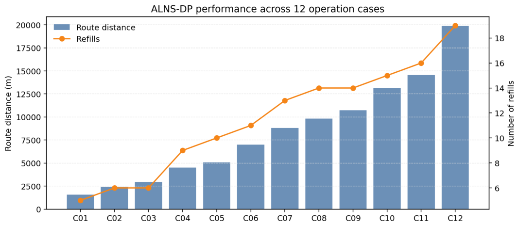
summarizes the best ALNS-DP schedule selected from ten runs for each operation case. This table reports the best schedule from the ten runs. Figure 5 visualizes the corresponding route-distance and replenishment-frequency trends. The number of cracks ranges from 18 to 64, and every crack is included in the schedule. As the work zone grows, the route distance, makespan, and replenishment distance increase accordingly. Material utilization remains stable; the final row reports a mean utilization of 83.1%, which indicates that the replenishment-triggered route segmentation uses the robot tank effectively.

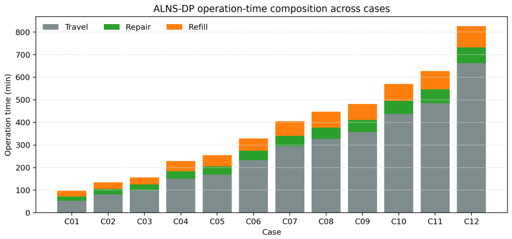
Figure 6 decomposes the best ALNS-DP schedule into travel, repair, and replenishment time. Travel is the dominant and most variable component, confirming that the main benefit of scheduling optimization is to reduce repeated traversals between spatially separated cracks and the replenishment point.

Table 13. Algorithm comparison on the representative case Case-08. Values are means over ten runs, and all methods repair all 46 cracks.

Method	Dist.	Span	Travel	Repair	Refill	Ref.	Util.	CPU
NNG	10,451.7	468.4	348.4	50.0	70.0	14.0	80.0	0.000
PFG	15,431.6	634.4	514.4	50.0	70.0	14.0	80.0	0.000
SWP	10,451.7	468.4	348.4	50.0	70.0	14.0	80.0	0.000
RAG	12,564.4	538.8	418.8	50.0	70.0	14.0	80.0	0.001
ALNS0	10,485.2	469.5	349.5	50.0	70.0	14.0	80.0	0.030
ALNS-DP	9861.6	448.7	328.7	50.0	70.0	14.0	80.0	4.336

gives the detailed operational indicators for the representative medium-large case Case-08, averaged over ten runs. This table reports ten-run means, whereas Table 12 reports the best schedule selected from ten runs; this distinction explains why the Case-08 route distance is 9823.1 m in Table 12 and 9861.6 m in Table 13. ALNS-DP reduces route distance and makespan compared with the greedy baselines while preserving the same full-completion rule. Relative to ALNS₀, ALNS-DP reduces the Case-08 route distance by 5.95%, makespan by 4.43%, and final objective by 6.86%. Travel, repair, and refill times are reported separately. Repair time and refill time are identical for the deterministic completion rule when all algorithms repair the same cracks and use the same number of replenishments; the performance difference therefore comes mainly from travel time and replenishment-related travel distance.

5.5. Dispatch Path Visualization

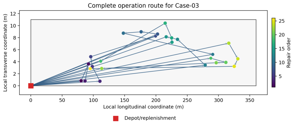
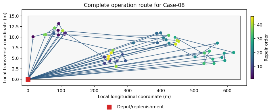
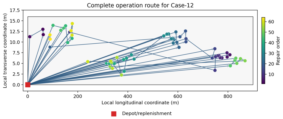
Figure 7, Figure 8 and Figure 9 show three ALNS-DP operation paths for small, medium-large, and large cases. All visible crack points are scheduled and repaired; no unplanned crack is left outside the route. The paths contain repeated returns to the replenishment point, which reflects the field process. The robot must replenish no later than the point at which the remaining sealant is insufficient for the next crack; during offline scheduling, an earlier capacity-feasible replenishment may be planned when it reduces the total operational objective.

5.6. Gantt Chart and Material Inventory

Table 14. Detailed ALNS-DP operational indicators for Case-08.

Indicator	Value
Repaired cracks	46/46
Completion rate	100.0%
Route distance	9823.1 m
Travel time	327.4 min
Repair time	50.0 min
Refill time	70.0 min
Replenishment trips	14
Replenishment-related distance	3967.0 m
Sealant consumption	60.01 L
Material utilization	80.0%

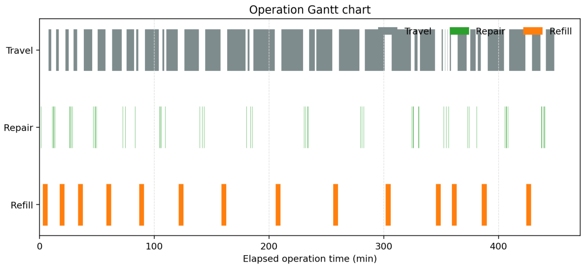
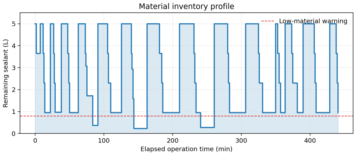
reports the operational metrics of the best ALNS-DP schedule for Case-08. Figure 10 shows the corresponding operation timeline, and Figure 11 shows the remaining sealant profile. The robot repairs all 46 cracks, has an estimated sealant demand of 60.01 L, and uses 14 replenishments. The total travel, repair, and refill times are 327.4, 50.0, and 70.0 min, respectively, yielding a makespan of 447.4 min.

6. Discussion

The proposed formulation connects robotic pavement repair with full-task operation scheduling and resource-renewal optimization. The main operational implication is that crack repair robots should not be evaluated only by perception accuracy or nozzle tracking error. Once a robot operates over a road segment with many cracks, its productivity also depends on route-level decisions: which crack should be repaired next, whether the remaining sealant can support the next service, and when the robot should return to the replenishment point.

The 12 case-study results show why replenishment-point design and replenishment timing should be evaluated explicitly. Every crack is repaired, so the comparison concerns the travel, return distance, and total work time required for the same operation. The ten-run tables, objective boxplot, objective heatmap, CPU profile, Wilcoxon test, ablation table, and weight-sensitivity analysis provide a broader view of performance and stability than a single representative example. The revised exact-MIP benchmark, Friedman test, Bonferroni-corrected post-hoc tests, demand-error sensitivity, replenishment-location sensitivity, and decoder-scaling test further clarify solution quality, statistical strength, robustness, and computational limits. The three operation-path maps, operation-time composition chart, Gantt chart, and material-inventory curve make the solution easier to audit: decision makers can see where the robot travels, when it repairs, when it replenishes, and how close it comes to the material-warning threshold.

The replenishment-location sensitivity has a direct engineering implication. When the supply point is fixed at an entrance, long work zones can produce repeated backtracking. A central temporary supply location can substantially reduce return distance if traffic control, material storage, and safety rules permit such a layout. Therefore, in practical deployment, agencies should treat the replenishment point as a design variable whenever it is not physically fixed by the site entrance or by material-handling constraints.

Several limitations remain. First, the case records are anonymized and transformed into local coordinate systems; broader external benchmarking will require additional shared datasets from other sites. Second, the current validation is a single-site study; additional sites with different road widths, crack densities, and traffic-control policies are needed for broader statistical validation. Third, field crews in current practice do not plan crack sequencing and replenishment timing as a predetermined schedule; decisions are instead made reactively on site based on visual inspection of remaining material, so no documented manual route or time budget exists for direct comparison with the offline-optimized ALNS-DP schedule. The deterministic NNG, PFG, SWP, and RAG rules are therefore used as reproducible engineering baselines that approximate common reactive sequencing logic (nearest-task, priority-first, spatial sweep, and refill-aware greedy), rather than as a claim of superiority over a specific historical manual plan. Fourth, the current robot platform does not directly measure crack depth, and the case study uses an engineering depth estimate for material-demand calculation. Fifth, the distance matrix is based on Euclidean distances in transformed local coordinates and does not yet account for road-network topology, obstacles, turning radii, or robot kinematic constraints. The impact of missed cracks was not quantified in this study and is left for future work because it depends on perception-level omission statistics rather than on the scheduling model itself. Sixth, the quality model is deliberately simple and is treated as an extension in the mandatory-repair experiments; a practical deployment should calibrate sealant temperature, crack-wall heating, surface moisture, and curing constraints. Finally, the current model assumes a single robot and a known crack map. Multi-robot coordination, online discovery, three-dimensional crack-volume perception, and road-network/kinodynamic distance modeling are natural extensions.

7. Conclusions

This paper developed a replenishment-aware operation scheduling model for a single asphalt crack repair robot. SACRP integrates mandatory crack repair, sealant capacity, fixed replenishment points, and operation-time indicators in a unified optimization framework. A compact MIP model was presented, NP-hardness was established, and an ALNS-DP heuristic was proposed to combine adaptive sequence search with replenishment-feasible route segmentation for fixed sequences.

The real case set contains 12 operation zones with 18–64 cracks per case. Six algorithms are evaluated on every case with ten runs each. ALNS-DP schedules every crack in each case and reduces the mean final objective by 5.11% relative to ALNS₀ on average. The representative Case-08 shows a 6.86% objective reduction, and small exact MIP benchmarks show 0.00% optimality gaps on 8–12 crack instances. The revised robustness analyses indicate that route efficiency is sensitive to replenishment-point placement and demand-estimation error, while the decoder-scaling test shows that a single DP pass remains fast up to 500 cracks. Future work will add more real sites, collect manual schedule baselines where field records permit, strengthen field-data validation, calibrate the material-consumption and quality models with measured sealant use, incorporate depth sensing or three-dimensional crack-volume estimation, and extend the approach to road-network-aware and multi-robot crack repair.

References

- Min, W.; Lu, P.; Liu, S.; Wang, H. A review of crack sealing technologies for asphalt pavement: Materials, failure mechanisms, and detection methods. Coatings 2025, 15, 836. [Google Scholar] [CrossRef] [Scilit]
- Liu, C.; Wang, H.; Liu, S.; Yang, D.; Xiong, Y. Performance evaluation of asphalt-pavement crack-repair materials. Materials 2025, 18, 1611. [Google Scholar] [CrossRef] [Scilit] [PubMed]
- Ai, D.; Jiang, G.; Lam, S.-K.; He, P.; Li, C. Computer vision framework for crack detection of civil infrastructure—A review. Eng. Appl. Artif. Intell. 2023, 117, 105478. [Google Scholar] [CrossRef] [Scilit]
- Lau, S.L.H.; Chong, E.K.P.; Yang, X.; Wang, X. Automated pavement crack segmentation using U-Net-based convolutional neural network. IEEE Access 2020, 8, 114892–114899. [Google Scholar] [CrossRef] [Scilit]
- Han, C.; Ma, T.; Huyan, J.; Huang, X.; Zhang, Y. CrackW-Net: A novel pavement crack image segmentation convolutional neural network. IEEE Trans. Intell. Transp. Syst. 2022, 23, 22135–22144. [Google Scholar] [CrossRef] [Scilit]
- Guo, F.; Qian, Y.; Liu, J.; Yu, H. Pavement crack detection based on transformer network. Autom. Constr. 2023, 145, 104646. [Google Scholar] [CrossRef] [Scilit]
- Han, B.; Zhang, Y.; Huang, C.; Ding, W.; Liu, Z.; Deng, H.; Wu, J. UMDA: Lightweight and efficient crack segmentation model. J. Comput. Civ. Eng. 2026, 40, 04025143. [Google Scholar] [CrossRef] [Scilit]
- Poudel, O.; Hu, X.; Assaad, R.H.; Wang, W.; Huang, T.; Wang, G. VTECSeg: Edge-aware hybrid CNN-vision transformer network with zero-shot vision-language-guided region proposals for crack segmentation. Autom. Constr. 2026, 188, 106998. [Google Scholar] [CrossRef] [Scilit]
- Chen, Y.; Zhu, Z.; Lin, Z.; Zhou, Y. Building surface crack detection using deep learning technology. Buildings 2023, 13, 1814. [Google Scholar] [CrossRef] [Scilit]
- Wu, J.; He, Y.; Xu, C.; Jia, X.; Huang, Y.; Chen, Q.; Huang, C.; Dadras Eslamlou, A.; Huang, S. Interpretability analysis of convolutional neural networks for crack detection. Buildings 2023, 13, 3095. [Google Scholar] [CrossRef] [Scilit]
- Jin, T.; Zhang, W.; Chen, C.; Chen, B.; Zhuang, Y.; Zhang, H. Deep-learning- and unmanned aerial vehicle-based structural crack detection in concrete. Buildings 2023, 13, 3114. [Google Scholar] [CrossRef] [Scilit]
- Qi, Y.; Ding, Z.; Luo, Y.; Ma, Z. A three-step computer vision-based framework for concrete crack detection and dimensions identification. Buildings 2024, 14, 2360. [Google Scholar] [CrossRef] [Scilit]
- Zhang, J.; Yang, X.; Wang, W.; Wang, H.; Ding, L.; El-Badawy, S.; You, Z. Vision-guided robot for automated pixel-level pavement crack sealing. Autom. Constr. 2024, 168, 105783. [Google Scholar] [CrossRef] [Scilit]
- Veeraraghavan, V.; Hunte, K.; Yi, J.; Yu, K. Complete and near-optimal robotic crack coverage and filling in civil infrastructure. IEEE Trans. Robot. 2024, 40, 2850–2867. [Google Scholar] [CrossRef] [Scilit]
- Xiao, B.; Chen, C.; Yin, X. Recent advancements of robotics in construction. Autom. Constr. 2022, 144, 104591. [Google Scholar] [CrossRef] [Scilit]
- Liu, Y.; Alias, A.H.; Haron, N.A.; Bakar, N.A.; Wang, H. Robotics in the construction sector: Trends, advances, and challenges. J. Intell. Robot. Syst. 2024, 110, 72. [Google Scholar] [CrossRef] [Scilit]
- Choset, H. Coverage for robotics–A survey of recent results. Ann. Math. Artif. Intell. 2001, 31, 113–126. [Google Scholar] [CrossRef] [Scilit]
- Sánchez-Ibáñez, J.R.; Pérez-del-Pulgar, C.J.; García-Cerezo, A. Path planning for autonomous mobile robots: A review. Sensors 2021, 21, 7898. [Google Scholar] [CrossRef] [Scilit] [PubMed]
- Vansteenwegen, P.; Souffriau, W.; Van Oudheusden, D. The orienteering problem: A survey. Eur. J. Oper. Res. 2011, 209, 1–10. [Google Scholar] [CrossRef] [Scilit]
- Dantzig, G.B.; Ramser, J.H. The truck dispatching problem. Manag. Sci. 1959, 6, 80–91. [Google Scholar] [CrossRef] [Scilit]
- Solomon, M.M. Algorithms for the vehicle routing and scheduling problems with time window constraints. Oper. Res. 1987, 35, 254–265. [Google Scholar] [CrossRef] [Scilit]
- Tarantilis, C.D.; Zachariadis, E.E.; Kiranoudis, C.T. A hybrid guided local search for the vehicle-routing problem with intermediate replenishment facilities. INFORMS J. Comput. 2008, 20, 154–168. [Google Scholar] [CrossRef] [Scilit]
- Kucukoglu, I.; Dewil, R.; Cattrysse, D. The electric vehicle routing problem and its variations: A literature review. Comput. Ind. Eng. 2021, 161, 107650. [Google Scholar] [CrossRef] [Scilit]
- Avolio, M.; Di Francesco, M.; Fuduli, A.; Gorgone, E.; Wolfler Calvo, R. Multi-day routes in a multi-depot vehicle routing problem with intermediate replenishment facilities and time windows. Comput. Oper. Res. 2025, 182, 107084. [Google Scholar] [CrossRef] [Scilit]
- Ropke, S.; Pisinger, D. An adaptive large neighborhood search heuristic for the pickup and delivery problem with time windows. Transp. Sci. 2006, 40, 455–472. [Google Scholar] [CrossRef] [Scilit]
- Voigt, S. A review and ranking of operators in adaptive large neighborhood search for vehicle routing problems. Eur. J. Oper. Res. 2025, 322, 357–375. [Google Scholar] [CrossRef] [Scilit]
- Jafarian Kafshgarkolaei, H.; Lotfollahi-Yaghin, M.A.; Mojtahedi, A. A modified orthonormal polynomial series expansion tailored to thin beams undergoing slamming loads. Ocean Eng. 2019, 182, 38–47. [Google Scholar] [CrossRef] [Scilit]
- Beasley, J.E. Route first–cluster second methods for vehicle routing. Omega 1983, 11, 403–408. [Google Scholar] [CrossRef] [Scilit]
- Miller, C.E.; Tucker, A.W.; Zemlin, R.A. Integer programming formulation of traveling salesman problems. J. ACM 1960, 7, 326–329. [Google Scholar] [CrossRef] [Scilit]
Figure 1.
Schematic overview of the single-robot crack repair scheduling problem with mandatory crack completion and replenishment-point returns.
Figure 2.
Boxplot of normalized final objective values over 12 cases and ten runs per algorithm. The dashed horizontal line marks the case-best normalization baseline.
Figure 3.
Heatmap of normalized mean objective values by case and algorithm. Values are normalized by the best mean objective in each case.
Figure 4.
CPU-time profile of ALNS0 and ALNS-DP over the 12 cases. The secondary axis reports the number of cracks.
Figure 5.
Route distance and replenishment frequency across the 12 operation cases.
Figure 6.
Operation-time composition of the best ALNS-DP schedules across the 12 cases.
Figure 7.
Complete ALNS-DP operation path for Case-03. Colors indicate repair order, and every displayed crack belongs to the executed schedule.
Figure 8.
Complete ALNS-DP operation path for Case-08. The route includes replenishment returns before the robot resumes crack repair.
Figure 9.
Complete ALNS-DP operation path for Case-12. The larger work zone produces more replenishment-linked route segments.
Figure 10.
Gantt chart of the ALNS-DP schedule for Case-08. The plotted bars do not overlap in a way that affects readability.
Figure 11.
Remaining sealant profile during the ALNS-DP schedule. Each upward jump corresponds to a replenishment operation, and the dashed line marks the low-material warning threshold.