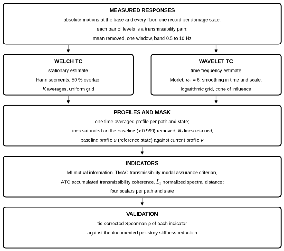
Figure 1.
Processing workflow from measured floor responses to the four damage indicators and the severity assessment.
Figure 1.
Processing workflow from measured floor responses to the four damage indicators and the severity assessment.
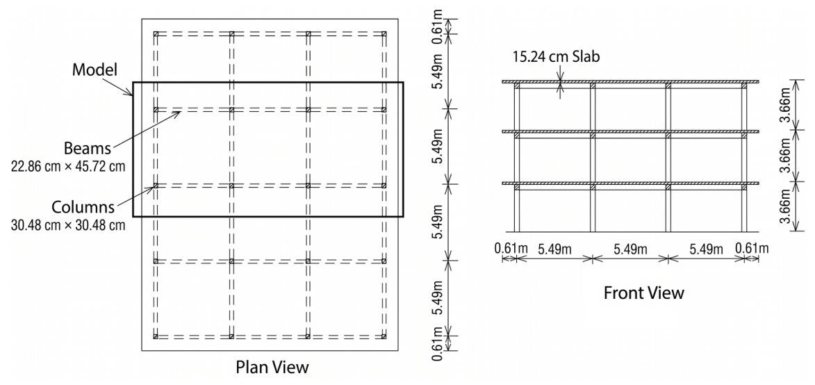
Figure 2.
Layout of the idealized prototype building underlying Cases I and II. Adapted from [
6].
Figure 2.
Layout of the idealized prototype building underlying Cases I and II. Adapted from [
6].
Figure 3.
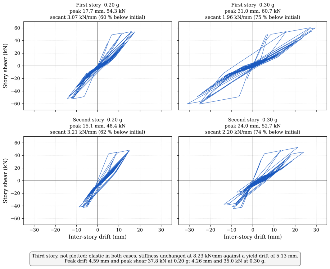
Computed story shear against inter-story drift of the baseline frame at 0.20 g and 0.30 g, showing the pinched, degrading hysteresis calibrated to the experimental program.
Figure 3.
Computed story shear against inter-story drift of the baseline frame at 0.20 g and 0.30 g, showing the pinched, degrading hysteresis calibrated to the experimental program.
Figure 4.
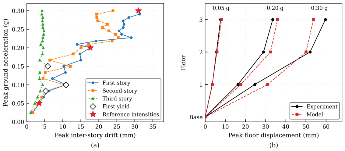
Case I model under the incrementally scaled Taft N21E record. (a) Peak inter-story drift against peak ground acceleration (PGA). (b) Peak floor displacement profiles at 0.05, 0.20, and 0.30 g.
Figure 4.
Case I model under the incrementally scaled Taft N21E record. (a) Peak inter-story drift against peak ground acceleration (PGA). (b) Peak floor displacement profiles at 0.05, 0.20, and 0.30 g.
Figure 5.
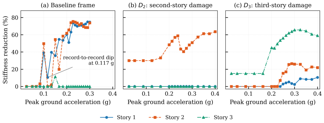
Per-story stiffness reduction against peak ground acceleration for the three configurations.
Figure 5.
Per-story stiffness reduction against peak ground acceleration for the three configurations.
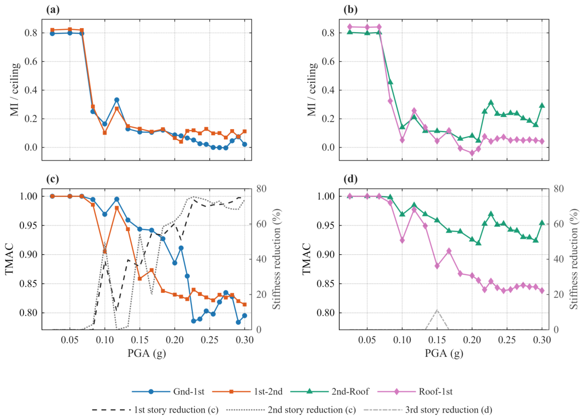
Figure 6.
Wavelet domain, baseline frame, MI as a fraction of its ceiling (Equation (
A5)), and TMAC against peak ground acceleration. (
a,
c) Paths Gnd–1st and 1st–2nd. (
b,
d) Paths 2nd–Roof and Roof–1st. The per-story stiffness reduction is overlaid on the right axis of Panels (
c,
d).
Figure 6.
Wavelet domain, baseline frame, MI as a fraction of its ceiling (Equation (
A5)), and TMAC against peak ground acceleration. (
a,
c) Paths Gnd–1st and 1st–2nd. (
b,
d) Paths 2nd–Roof and Roof–1st. The per-story stiffness reduction is overlaid on the right axis of Panels (
c,
d).
Figure 7.
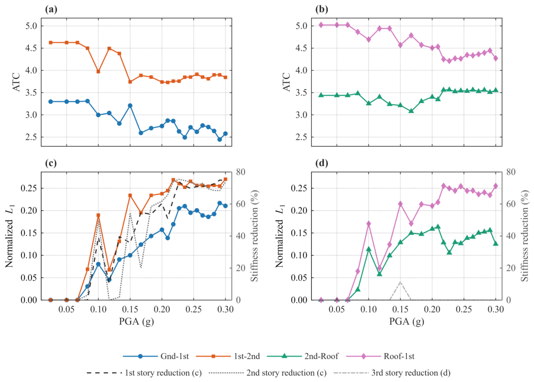
Wavelet domain, baseline frame, ATC, and against peak ground acceleration; (a,c) Paths Gnd–1st and 1st–2nd. (b,d) Paths 2nd–Roof and Roof–1st. The per-story stiffness reduction is overlaid on the right axis of Panels (c,d).
Figure 7.
Wavelet domain, baseline frame, ATC, and against peak ground acceleration; (a,c) Paths Gnd–1st and 1st–2nd. (b,d) Paths 2nd–Roof and Roof–1st. The per-story stiffness reduction is overlaid on the right axis of Panels (c,d).
Figure 8.
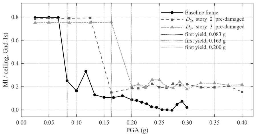
Mutual information on the wavelet Gnd–1st path, as a fraction of its ceiling (Equation (
A5)), against peak ground acceleration for the three configurations; dotted lines mark first yield.
Figure 8.
Mutual information on the wavelet Gnd–1st path, as a fraction of its ceiling (Equation (
A5)), against peak ground acceleration for the three configurations; dotted lines mark first yield.
Figure 9.
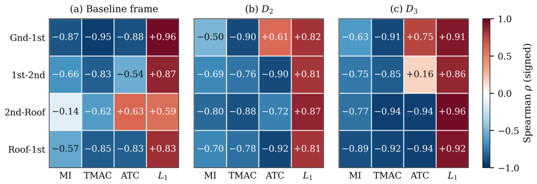
Wavelet domain, signed tie-corrected Spearman rank correlation of the four indicators against the reference stiffness reduction: (a) the baseline frame, referenced to story one; (b) , in which only the second story degrades; (c) , in which the third story is the most damaged.
Figure 9.
Wavelet domain, signed tie-corrected Spearman rank correlation of the four indicators against the reference stiffness reduction: (a) the baseline frame, referenced to story one; (b) , in which only the second story degrades; (c) , in which the third story is the most damaged.
Figure 10.
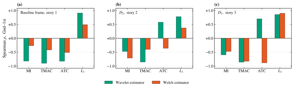
Ground-to-first-floor severity correlation of the four indicators, wavelet against Welch, on absolute accelerations for the three configurations (a–c).
Figure 10.
Ground-to-first-floor severity correlation of the four indicators, wavelet against Welch, on absolute accelerations for the three configurations (a–c).
Figure 11.
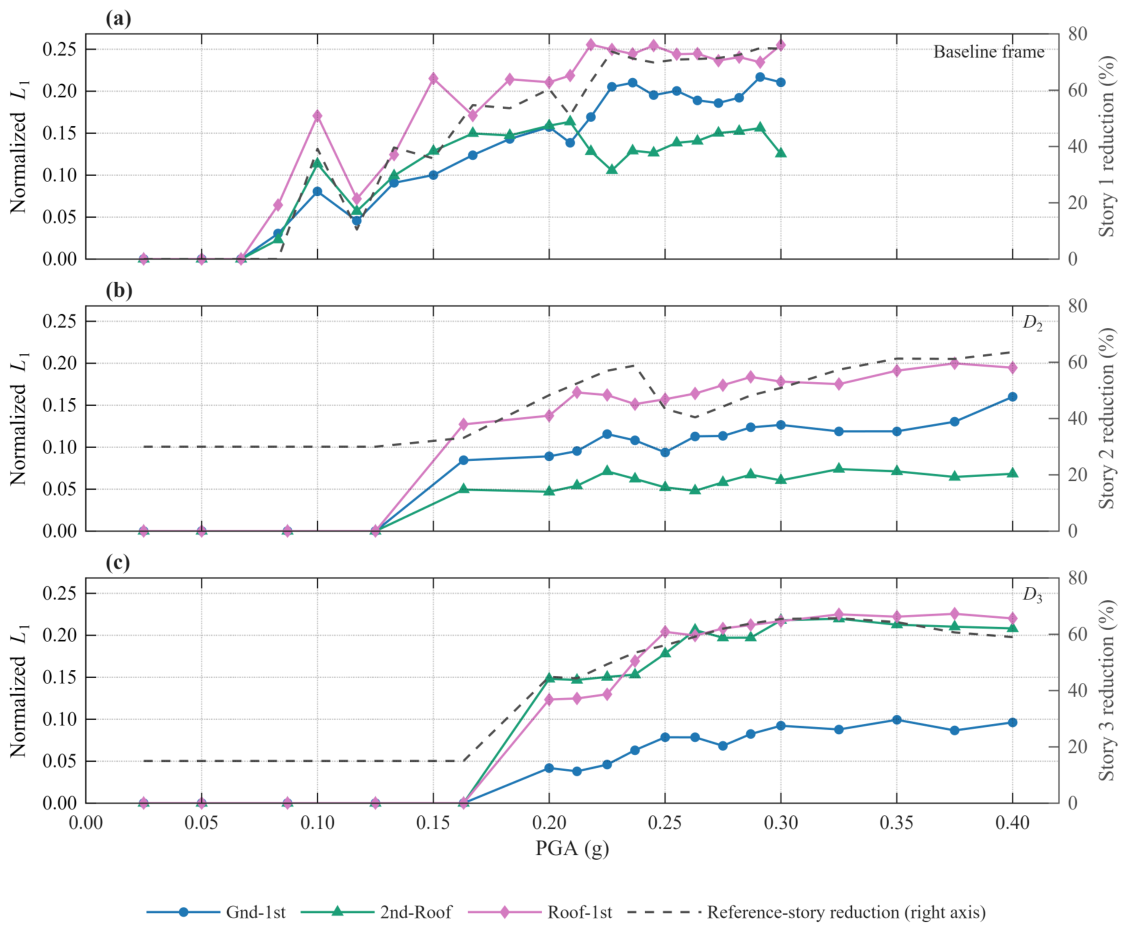
Wavelet domain, on three paths, left axis, with the reference-story stiffness reduction, right axis, against peak ground acceleration: (a) the baseline frame, (b) , (c) .
Figure 11.
Wavelet domain, on three paths, left axis, with the reference-story stiffness reduction, right axis, against peak ground acceleration: (a) the baseline frame, (b) , (c) .
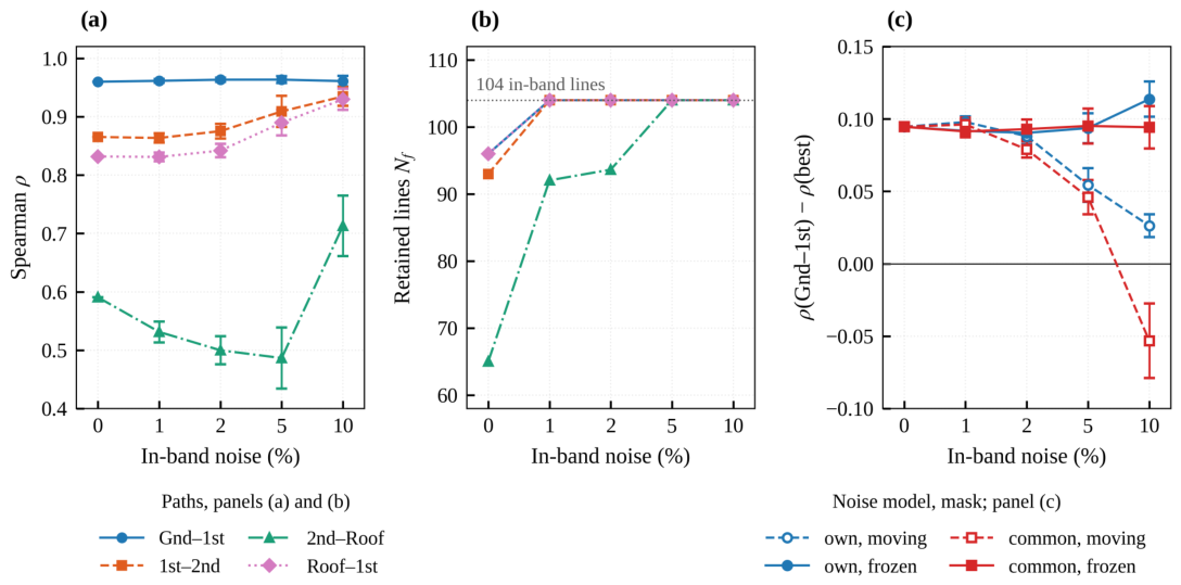
Figure 12.
Measurement-noise sensitivity of Case I. (a) Severity correlation of and (b) retained lines, both for own-channel noise with the threshold recomputed. (c) Margin, for both noise models and both mask treatments. Error bars: one standard deviation over the realizations in (a), twice the standard error of the paired difference in (c).
Figure 12.
Measurement-noise sensitivity of Case I. (a) Severity correlation of and (b) retained lines, both for own-channel noise with the threshold recomputed. (c) Margin, for both noise models and both mask treatments. Error bars: one standard deviation over the realizations in (a), twice the standard error of the paired difference in (c).
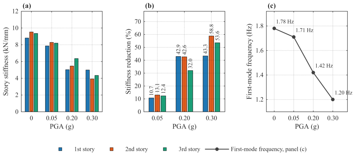
Figure 13.
Case II damage reference, from the white-noise identification after each test. (a) Story stiffness, (b) cumulative reduction from the undamaged state, (c) first-mode frequency.
Figure 13.
Case II damage reference, from the white-noise identification after each test. (a) Story stiffness, (b) cumulative reduction from the undamaged state, (c) first-mode frequency.
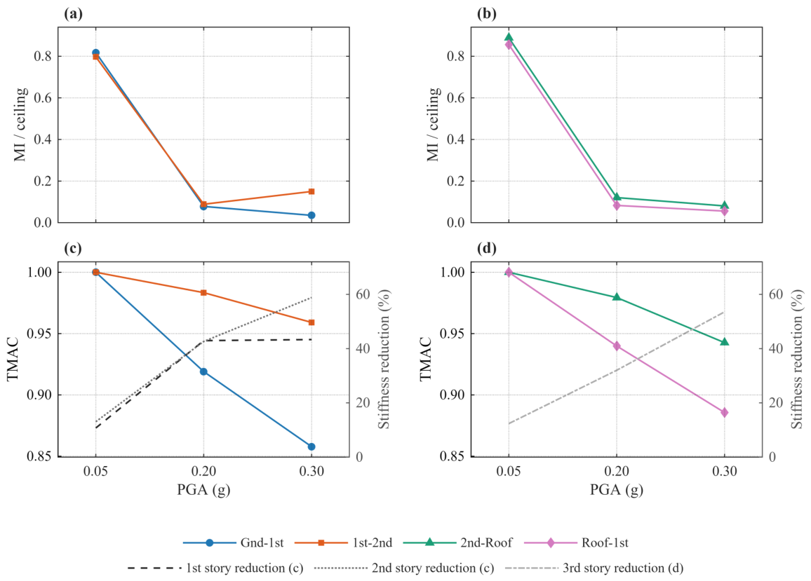
Figure 14.
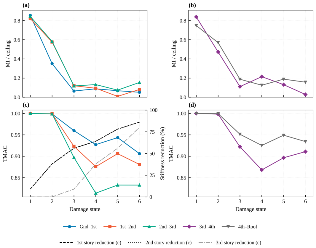
Experimental shake-table tests, MI and TMAC across the three tests. Panels (a,c) show the Gnd–1st and 1st–2nd paths, Panels (b,d) the 2nd–Roof and Roof–1st paths; the measured reduction in the spanned stories is overlaid on Panels (c,d).
Figure 14.
Experimental shake-table tests, MI and TMAC across the three tests. Panels (a,c) show the Gnd–1st and 1st–2nd paths, Panels (b,d) the 2nd–Roof and Roof–1st paths; the measured reduction in the spanned stories is overlaid on Panels (c,d).
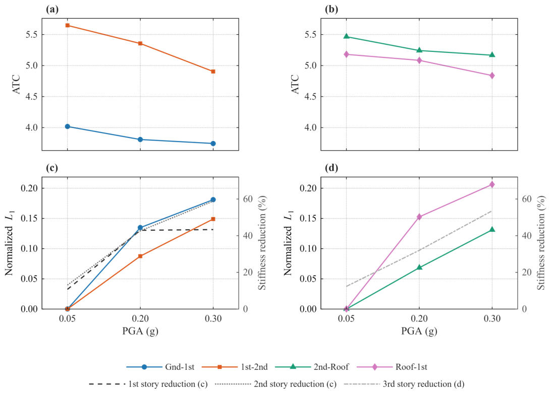
Figure 15.
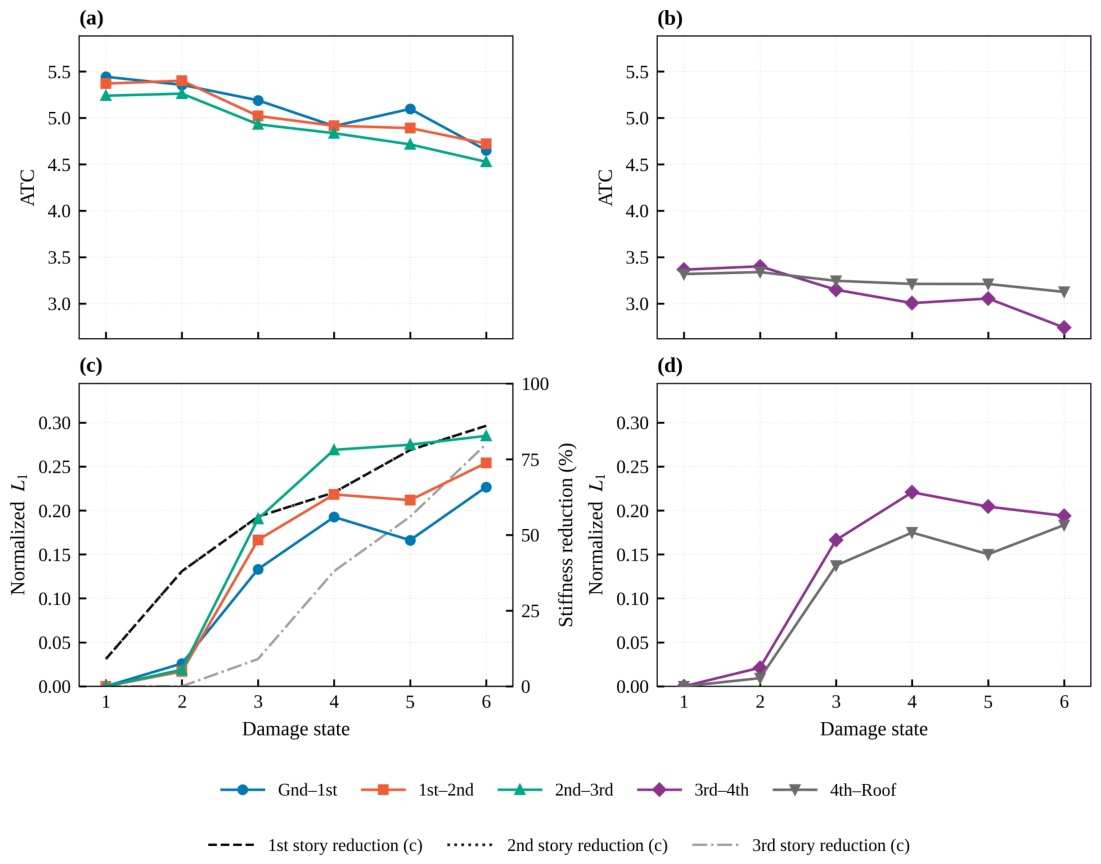
Experimental shake-table tests, ATC and
across the three tests; layout and overlay as in
Figure 14. Panels (
a,
c) show the Gnd–1st and 1st–2nd paths, Panels (
b,
d) the 2nd–Roof and Roof–1st paths; the measured reduction in the spanned stories is overlaid on Panels (
c,
d).
Figure 15.
Experimental shake-table tests, ATC and
across the three tests; layout and overlay as in
Figure 14. Panels (
a,
c) show the Gnd–1st and 1st–2nd paths, Panels (
b,
d) the 2nd–Roof and Roof–1st paths; the measured reduction in the spanned stories is overlaid on Panels (
c,
d).
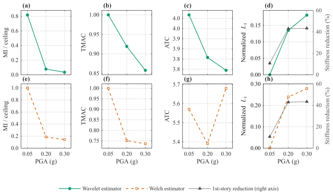
Figure 16.
Experimental shake-table tests, Gnd–1st path. The four indicators across the three tests, wavelet estimator (top row (a–c)) and Welch estimator (bottom row (e–g)); L1 panels (d,h), the first-story reduction is overlaid on the panels.
Figure 16.
Experimental shake-table tests, Gnd–1st path. The four indicators across the three tests, wavelet estimator (top row (a–c)) and Welch estimator (bottom row (e–g)); L1 panels (d,h), the first-story reduction is overlaid on the panels.
Figure 17.
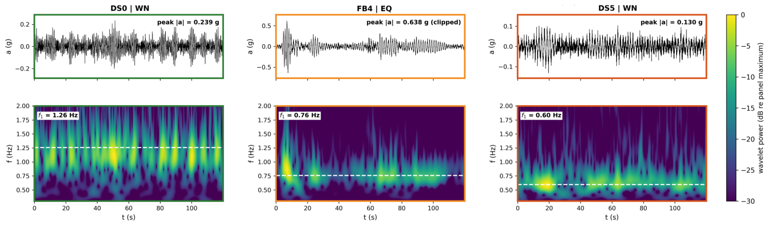
Three of the sixteen Case III tests, recorded acceleration (
top) and wavelet power below 3 Hz (
bottom): the undamaged characterization DS0, the earthquake FB4, and the characterization after FB5 (DS5). The panel border color indicates the damage state, and the dashed line is the first-mode frequency of
Table 2.
Figure 17.
Three of the sixteen Case III tests, recorded acceleration (
top) and wavelet power below 3 Hz (
bottom): the undamaged characterization DS0, the earthquake FB4, and the characterization after FB5 (DS5). The panel border color indicates the damage state, and the dashed line is the first-mode frequency of
Table 2.
Figure 18.
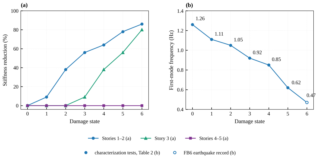
Case III damage reference: (
a) per-story secant-stiffness reduction identified in [
19]; (
b) first-mode frequency versus damage state from the base-to-roof transfer function (
Table 2), DS6 from the FB6 record.
Figure 18.
Case III damage reference: (
a) per-story secant-stiffness reduction identified in [
19]; (
b) first-mode frequency versus damage state from the base-to-roof transfer function (
Table 2), DS6 from the FB6 record.
Figure 19.
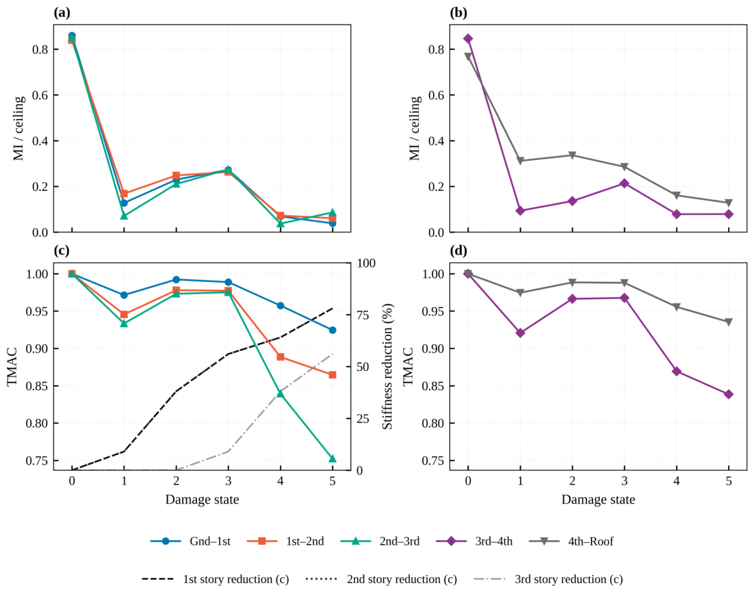
Case III, white-noise set: floor-averaged MI (a,b) and TMAC (c,d) against damage state. (a,c) paths spanning softened stories, with the documented reduction overlaid on (c); (b,d) paths spanning intact stories.
Figure 19.
Case III, white-noise set: floor-averaged MI (a,b) and TMAC (c,d) against damage state. (a,c) paths spanning softened stories, with the documented reduction overlaid on (c); (b,d) paths spanning intact stories.
Figure 20.
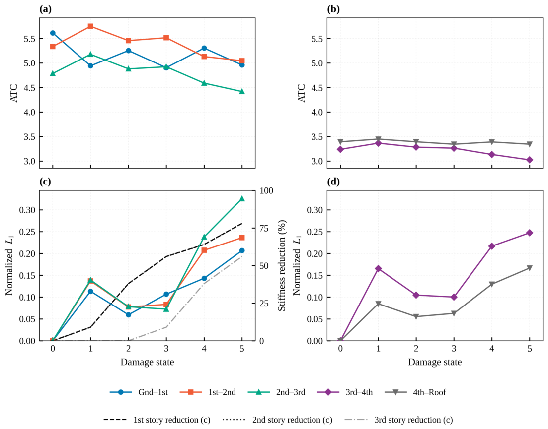
Case III, white-noise set. Floor-averaged ATC (
a,
b) and
(
c,
d); layout, path groups and overlay as in
Figure 19.
Figure 20.
Case III, white-noise set. Floor-averaged ATC (
a,
b) and
(
c,
d); layout, path groups and overlay as in
Figure 19.
Figure 21.
Case III, earthquake set. Floor-averaged MI and TMAC along the damage progression produced by FB1–FB6 (DS1–DS6), one test per state, same layout and overlay as
Figure 19. Case III, white-noise set: floor-averaged MI (
a,
b) and TMAC (
c,
d) against damage state.
Figure 21.
Case III, earthquake set. Floor-averaged MI and TMAC along the damage progression produced by FB1–FB6 (DS1–DS6), one test per state, same layout and overlay as
Figure 19. Case III, white-noise set: floor-averaged MI (
a,
b) and TMAC (
c,
d) against damage state.
Figure 22.
Case III, earthquake set. Floor-averaged ATC and
, same layout and overlay as
Figure 19. Case III, white-noise set: floor-averaged MI (
a,
b) and TMAC (
c,
d) against damage state.
Figure 22.
Case III, earthquake set. Floor-averaged ATC and
, same layout and overlay as
Figure 19. Case III, white-noise set: floor-averaged MI (
a,
b) and TMAC (
c,
d) against damage state.
Figure 23.
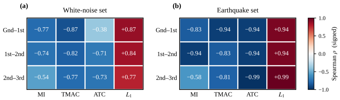
Case III, signed tie-corrected Spearman correlation between each indicator and the own-story secant-stiffness reduction, on the three paths spanning softened stories (a,b). No coefficient is defined on 3rd–4th and 4th–Roof, whose stories stay at baseline.
Figure 23.
Case III, signed tie-corrected Spearman correlation between each indicator and the own-story secant-stiffness reduction, on the three paths spanning softened stories (a,b). No coefficient is defined on 3rd–4th and 4th–Roof, whose stories stay at baseline.
Figure 24.
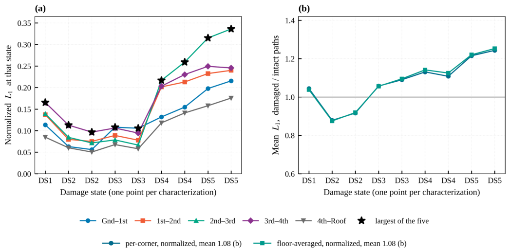
Single-state localization on Case III, white-noise set. (a) Normalized of each path at every characterization, the largest of the five starred. (b) Mean on the three damaged paths over the mean on the two intact paths, floor-averaged and per corner.
Figure 24.
Single-state localization on Case III, white-noise set. (a) Normalized of each path at every characterization, the largest of the five starred. (b) Mean on the three damaged paths over the mean on the two intact paths, floor-averaged and per corner.
Figure 25.
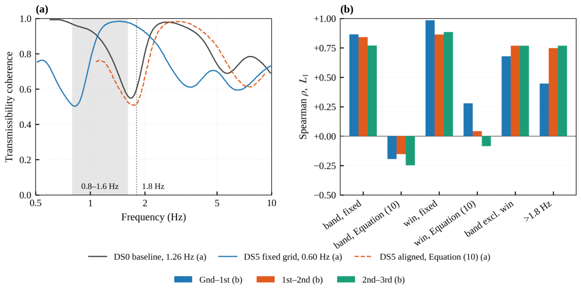
Case III, white-noise set. (
a) Wavelet transmissibility coherence on Gnd–1st: the DS0 baseline at 1.26 Hz, the DS5 record at 0.60 Hz on the fixed grid, and the same DS5 profile mapped by Equation (
10); the shaded band is 0.8–1.6 Hz and the dotted line 1.8 Hz. (
b) Tie-corrected Spearman correlation of
with the own-story stiffness reduction on the three paths spanning softened stories, for the whole band and for the 0.8–1.6 Hz window on each abscissa, for the band with that window deleted, and for the lines above 1.8 Hz.
Figure 25.
Case III, white-noise set. (
a) Wavelet transmissibility coherence on Gnd–1st: the DS0 baseline at 1.26 Hz, the DS5 record at 0.60 Hz on the fixed grid, and the same DS5 profile mapped by Equation (
10); the shaded band is 0.8–1.6 Hz and the dotted line 1.8 Hz. (
b) Tie-corrected Spearman correlation of
with the own-story stiffness reduction on the three paths spanning softened stories, for the whole band and for the 0.8–1.6 Hz window on each abscissa, for the band with that window deleted, and for the lines above 1.8 Hz.
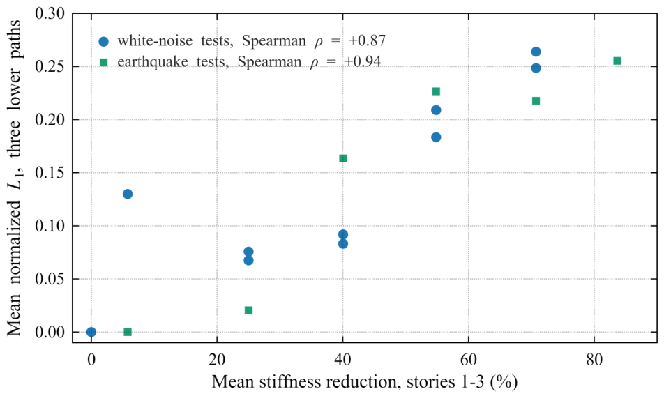
Figure 26.
Case III overall damage tracking. Mean of the three lower-story paths against the mean lower-story stiffness reduction; circles white-noise tests, squares earthquake tests; is the tie-corrected Spearman coefficient.
Figure 26.
Case III overall damage tracking. Mean of the three lower-story paths against the mean lower-story stiffness reduction; circles white-noise tests, squares earthquake tests; is the tie-corrected Spearman coefficient.
Table 1.
Saturation-threshold sensitivity of Case I.
is the number of the 104 in-band lines entering the indicators. The
column carries the sampling variability of the 200-permutation bias correction of MI (
Appendix A), about
; the adopted rows are those of the deposited run, from which every MI value in the text is quoted.
Table 1.
Saturation-threshold sensitivity of Case I.
is the number of the 104 in-band lines entering the indicators. The
column carries the sampling variability of the 200-permutation bias correction of MI (
Appendix A), about
; the adopted rows are those of the deposited run, from which every MI value in the text is quoted.
| Threshold | Path | | | | | |
|---|
| 0.99 | Gnd–1st | 84 | | | | |
| 1st–2nd | 66 | | | | |
| 2nd–Roof | 46 | | | | |
| Roof–1st | 76 | | | | |
| 0.995 | Gnd–1st | 90 | | | | |
| 1st–2nd | 78 | | | | |
| 2nd–Roof | 48 | | | | |
| Roof–1st | 84 | | | | |
| 0.999 (adopted) | Gnd–1st | 96 | | | | |
| 1st–2nd | 93 | | | | |
| 2nd–Roof | 65 | | | | |
| Roof–1st | 96 | | | | |
| none | Gnd–1st | 104 | | | | |
| 1st–2nd | 104 | | | | |
| 2nd–Roof | 104 | | | | |
| Roof–1st | 104 | | | | |
Table 2.
Case III, first-mode frequency and equivalent damping of every test, identified from the base-to-roof transfer function.
Table 2.
Case III, first-mode frequency and equivalent damping of every test, identified from the base-to-roof transfer function.
| Test a | Type | DS | (Hz) b | (%) c | Sub-Windows (%) d | | Median (Hz) f | 10–90% (Hz) g |
|---|
| 01 WN AA | WN | 0 | 1.258 | 3.3 | – | 0.97 | 1.254 | 1.016–1.433 |
| 02 CNP100 | EQ | 1 | 1.096 | 3.4 | 4.8–5.3 | 0.98 | 1.284 | 1.034–1.370 |
| 03 Pulse A | PULSE | 1 | 1.109 | 3.8 | – | 0.96 | 1.193 | 0.883–1.399 |
| 04 LAC100 | EQ | 2 | 1.077 | 3.7 | 3.0–4.6 | 0.94 | 1.235 | 1.000–1.513 |
| 05 Pulse B | PULSE | 2 | 1.053 | 3.4 | – | 0.94 | 1.310 | 0.935–1.517 |
| 06 Pulse C | PULSE | 2 | 1.057 | 3.8 | – | 0.97 | 1.315 | 1.030–1.320 |
| 07 ICA50 | EQ | 3 | 0.889 | 4.0 | 3.8–5.4 | 0.92 | 0.891 | 0.799–1.040 |
| 08 Pulse D | PULSE | 3 | 0.920 | 4.1 | – | 0.96 | 0.926 | 0.731–1.167 |
| 09 Pulse E | PULSE | 3 | 0.925 | 3.1 | – | 0.95 | 0.985 | 0.780–1.150 |
| 10 ICA100 | EQ | 4 | 0.761 | 4.2 | 3.0–4.0 | 0.92 | 0.733 | 0.670–0.834 |
| 11 WN F | WN | 4 | 0.862 | 5.9 | – | 0.94 | 0.833 | 0.734–0.933 |
| 12 WN G | WN | 4 | 0.829 | 4.7 | – | 0.94 | 0.821 | 0.690–0.917 |
| 13 DEN67 | EQ | 5 | 0.614 | 4.2 | 3.3–10.3 | 0.86 | 0.635 | 0.531–0.780 |
| 14 WN H | WN | 5 | 0.643 | 5.7 | – | 0.91 | 0.615 | 0.543–0.681 |
| 15 WN I | WN | 5 | 0.598 | 5.0 | – | 0.93 | 0.598 | 0.539–0.654 |
| 16 DEN100 | EQ | 6 | 0.474 | 15.2 g | 1.5–17.8 | 0.70 | 0.433 | 0.347–0.521 |
Table 3.
Severity correlation of on Case III under reduced instrumentation, and of against an amplitude-only benchmark on the transmissibility magnitude, by path.
Table 3.
Severity correlation of on Case III under reduced instrumentation, and of against an amplitude-only benchmark on the transmissibility magnitude, by path.
| (a) Instrumented Levels Retained a |
| Levels | Array | |
| 6 | full array | |
| 5 | all floors, no base | |
| 4 | base and alternate floors | |
| 3 | base, second floor, roof | |
| 2 | base and roof | |
| (b) Coherence Indicator Against the Amplitude Benchmark b |
| Case, Path | | |
| I, Gnd–1st (input-anchored) | | |
| I, 1st–2nd | | |
| I, 2nd–Roof | | |
| I, Roof–1st | | |
| III, Gnd–1st (input-anchored) | | |
| III, 1st–2nd | | |
| III, 2nd–3rd | | |
Table 4.
Pairwise between two Case III tests, on the DS0 support, for the Gnd–1st path and averaged over the three paths spanning softened stories.
Table 4.
Pairwise between two Case III tests, on the DS0 support, for the Gnd–1st path and averaged over the three paths spanning softened stories.
| Contrast | What Differs | Gnd–1st | Mean of Three |
|---|
| DS2, pulse B against C | nothing (repeat) | 0.017 | 0.016 |
| DS3, pulse D against E | nothing (repeat) | 0.013 | 0.015 |
| DS4, against | amplitude | 0.037 | 0.039 |
| DS5, against | amplitude | 0.035 | 0.043 |
| DS4 → DS5 at | state | 0.116 | 0.130 |
| DS4 → DS5 at | state | 0.117 | 0.136 |
| DS1 → DS2, pulse | state | 0.082 | 0.077 |
| DS2 → DS3, pulse | state | 0.056 | 0.037 |
| DS0 → DS4, / | cumulative | 0.132/0.155 | 0.183/0.209 |
| DS0 → DS5, / | cumulative | 0.198/0.216 | 0.249/0.264 |
| FB1 → FB2 | earthquake set | 0.026 | 0.021 |
| FB1 → FB3 | earthquake set | 0.134 | 0.167 |
| FB1 → FB4 | earthquake set | 0.194 | 0.232 |
| FB1 → FB5 | earthquake set | 0.167 | 0.223 |
| FB1 → FB6 | earthquake set | 0.226 | 0.260 |