Article

Property Value Assessment Under EU Banking Regulation

by
Giampiero Bambagioni
Department of Civil and Environmental Engineering, University of Perugia, 06125 Perugia, Italy
Buildings 2026, 16(18), 3688; https://doi.org/10.3390/buildings16183688
Submission received: 25 August 2026 / Revised: 12 September 2026 / Accepted: 14 September 2026 / Published: 16 September 2026
(This article belongs to the Section Architectural Design, Urban Science, and Real Estate)

Abstract

A methodological framework for real estate collateral under CRR3, taking into account the International Valuation Standards (IVS) and relevant ESG factors, including physical and environmental risks, in determining prudential value. The study includes illustrative numerical applications to property resilience and physical risks. This paper examines the methodological implications of property value (PV) under Article 229 of Regulation (EU) 2024/1623, which, in implementation of the Basel III framework, amended Regulation (EU) No 575/2013 on prudential requirements for credit institutions and investment firms, for real estate collateral valuation (CRR3). It considers how current market value (MV) may be tested against the value sustainable over the life of the loan, with particular attention to property resilience, energy efficiency and materially relevant environmental and physical risks. The study combines the CRR3 framework, European Banking Autority (EBA) Guidelines and European Central Bank (ECB) Good Practices with valuation standards and a targeted critical review of recent literature. Drawing on the IVS and the Italian property valuation standard, it proposes a market-capped and sustainability-tested framework for determining property value, in which risk-adjusted market value (MVRA) is used as an analytical variable to identify residual risk not already reflected in market prices. The Aphys formulation provides a first-order analytical representation of event-based physical and environmental risk adjustments through probability, uninsured property damage, property-level loss of use, non-overlapping restoration costs, discounting, and a residual-risk coefficient intended to control double counting. The framework is then applied to three hypothetical numerical worked cases in different Italian Regions: a residential property exposed to hydraulic risk in Emilia-Romagna, an income-producing commercial property exposed to seismic risk in the Marche, and a residential property with partial seismic improvement in Sicily (Messina). The cases include structured comparable analysis, illustrative scenario parameterization, and multivariate sensitivity analysis. They illustrate the computational mechanics and internal consistency of the proposed framework but do not constitute empirical calibration, validation, or evidence of real-world predictive performance; the residual-risk parameters still require calibration using observed market, hazard, vulnerability, insurance, and loss data. The framework may affect the exposure-to-value ratio (ETV) and, depending on the applicable prudential treatment, risk-weighted exposure amounts. The broader ESG perimeter recognized by valuation standards is also acknowledged: Social and Governance variables are not numerically parameterized in the three worked cases, but, where material, they should be mapped to transparent and non-duplicative valuation channels.

1. Introduction

The reform of the European prudential framework, originating in Basel III (the international regulatory framework for banks) and culminating in the publication of Regulation (EU) 2024/1623 amending Regulation (EU) No 575/2013 (Capital Requirements Regulation, CRR3) [1] and Directive (EU) 2024/1619 (CRD6) [2], introduced significant changes to the treatment of exposures secured by immovable property. In particular, Article 229 CRR3, applicable from 1 January 2025, introduces for valuation purposes: (i) prudently conservative valuation criteria for the value of the property (property value), specifying that “the value is appraised using prudently conservative valuation criteria”; (ii) market value, where it can be determined, as the upper limit; and (iii) an adjustment where current market value could be significantly above the value sustainable over the life of the loan: “the value is adjusted to take into account the potential for the current market value to be significantly above the value that would be sustainable over the life of the loan”.
CRR3 defines property value by reference to Article 229(1), but the professional interpretation of how that prudential value should be implemented is still developing. The IVSC statement of 28 April 2025 notes that there is no agreed implementation methodology and identifies three practices observed in Europe: mortgage lending value, an adjusted market value where the adjustment is determined by the valuer, and an adjusted market value where the adjustment is determined by the credit institution or a third-party data provider [3]. Accordingly, this paper presents a valuer-adjusted market value framework as one possible methodological interpretation; it does not claim to be the exclusive regulatory solution or to create a new IVS basis of value.
This regulatory innovation operates at the prudential level and must be read together with applicable valuation standards and professional requirements [4,5,6,7]. Property value requires a prudently conservative assessment that excludes expectations of price increases, tests whether current market value may be significantly above the value sustainable over the life of the loan, and documents the analysis transparently. This paper focuses on the environmental dimensions most directly connected with the real-estate collateral itself: property resilience, energy efficiency and physical risks. It does not purport to model social and governance factors comprehensively.
Physical and environmental risks relevant to a property are treated as exogenous hazards whose economic impacts depend on the asset’s exposure, vulnerability and resilience. Relevant physical risks may include hydrological and hydrogeological hazards (e.g., floods and landslides), and geophysical hazards (e.g., earthquakes and volcanic events), as well as other environmental factors such as noise and air pollution, wildfires, or the presence of contaminated sites and/or brownfield areas requiring remediation. In this context, a hazard represents the potentially damaging event or condition affecting a given area, whereas risk refers to its possible consequences, namely the foreseeable damage resulting from the interaction between hazard, exposure, and vulnerability (In financial-sector terminology, climate risks are generally grouped into two main categories: physical risks and transition risks. Physical risk is associated with the occurrence of extreme natural phenomena attributed by science to climate change. Transition risk arises from the shift toward new energy production and consumption systems designed to reduce greenhouse-gas emissions; accordingly, climate-change mitigation policies themselves may also be a source of risk. (Available online: https://www.bancaditalia.it/focus/sostenibilita/faq/index.html (accessed on 13 July 2026)).
The broader ESG perimeter recognized by IVS and the Codice delle Valutazioni Immobiliari (Italian Property Valuation Standard, IPVS) is wider than the subset modeled numerically in this paper. In particular, Chapter 5 and Annex A of the IPVS identify an indicative and non-exhaustive set of social factors, including workplace health and safety; socio-economic conditions such as demographic trends, economic context and sustainable-development prospects, inequality, poverty, crime and security; and data protection and privacy. Governance factors include the applicable sectoral legal and regulatory framework, the legal position of the owner or user, risk-governance and compliance arrangements, transparency and reporting [5]. These variables may become valuation-relevant where they have a demonstrable transmission channel to use, marketability, operating or compliance costs, expected cash flows or other components of property value.
This paper takes into account the applicable European banking framework [1,2], the International Valuation Standards [4], the Codice delle Valutazioni Immobiliari (Italian Property Valuation Standard) [5], and relevant European valuation guidance [6,7]. It has three objectives: (i) to analyze methodologically how PV may be determined, with specific reference to materially relevant physical risks; (ii) to propose a structured framework for identifying and quantifying residual risk not already incorporated into market value, including through the Aphys formulation; and (iii) to place the illustrative good practices set out in the ECB Good Practices for Climate and Nature Risk Management (May 2026) [8] within the binding CRR3 and applicable EBA Guidelines on the management of ESG Risks [9].

Research Question and Methodological Approach

Against this background, the research question is as follows: how can the requirement of Article 229 CRR3—which is intended to capture the potential divergence between current market value and the value sustainable over the life of the loan—be translated into a transparent analytical valuation framework that incorporates materially relevant physical risks without turning mere exposure into an automatic haircut and without duplicating risk components already incorporated into market prices?
The paper adopts a conceptual, methodological, and numerical approach. It combines: (i) legal and regulatory analysis of the relevant CRR3/CRD6 provisions [1,2]; (ii) a coordinated reading of the European Banking Autority (EBA) Guidelines [9] and European Central Bank (ECB) Good Practices [8], while distinguishing their different legal status; (iii) comparison with relevant valuation standards [4,5,6,7]; (iv) a targeted critical review of recent literature on the channels through which physical risks, energy efficiency and resilience may affect property values and credit risk; and (v) three illustrative numerical worked applications with structured comparable analysis and multivariate sensitivity testing. The framework remains a methodological proposal rather than a prescribed regulatory model or a complete catastrophe-loss model; the worked applications illustrate computational mechanics and internal coherence, while external empirical calibration and validation remain necessary.
The literature component is a targeted critical/narrative review rather than a formal systematic review. Sources were selected for direct relevance to property-value effects, physical-risk transmission channels, resilience, energy efficiency, insurance, and prudential collateral valuation. Peer-reviewed empirical studies are used to support empirical market propositions; primary legal, regulatory and supervisory materials establish normative status and supervisory context; professional valuation standards are used for methodological alignment. These source categories are therefore not treated as equivalent forms of empirical evidence.
The literature-identification process was conducted iteratively over approximately the twelve months preceding finalization of the manuscript (August 2025 to September 2026). Consistently with the targeted critical/narrative design, no formal systematic-review protocol or exhaustive search log was maintained. Relevant academic literature was identified through multiple bibliographic databases and academic search engines, direct searches of publisher repositories and working-paper platforms (including SSRN), and backward and forward citation tracing. Primary legal, regulatory, supervisory and technical materials were retrieved directly from EU/EUR-Lex, EBA, ECB, Basel Committee on Banking Supervision (BCBS), Bank for International Settlements (BIS), Organisation for Economic Co-operation and Development (OECD) and International Valuation Standard Council (IVSC) sources and, for hazard and property-level technical information, from relevant European and Italian public repositories such as JRC, Copernicus/Climate-ADAPT, ISPRA and INGV.
Search terms were combined iteratively rather than through a predetermined systematic-review string. They included, among others, combinations of ‘property value’, ‘CRR3’, ‘Article 229’, ‘prudential valuation’, ‘real estate collateral’, ‘physical risk’, ‘climate risk’, ‘flood risk’, ‘seismic risk’, ‘property value’, ‘house prices’, ‘market pricing’, ‘ESG risks’, ‘risk capitalization’, ‘resilience’, ‘energy efficiency’, ‘green premium’, ‘brown discount’, ‘hedonic pricing’, ‘commercial real estate’ and ‘mortgage rates’. Priority was given to recent literature relevant to the CRR3 and evolving physical-risk context, while earlier seminal studies were retained where necessary to establish well-documented valuation channels. The search was intended to identify directly relevant methodological and empirical evidence rather than to claim exhaustive coverage of the literature.
The regulatory logic of the proposed framework is intended for the EU prudential context because its constraints derive from CRR3. The Italian Property Valuation Standard and Italian hazard/data sources are used as illustrative national implementation references. Application in another Member State requires local evidence on valuation practice, market pricing, construction characteristics, hazard data, insurance conditions, and public mitigation; parameters should not be transferred across jurisdictions without validation.
The paper is structured as follows. Section 2 describes the regulatory, supervisory and literature sources used, the methodological gap and the design of the applied cases. Section 3 presents the proposed methodological framework and applies it to three worked cases with sensitivity analysis. Section 4 discusses the implications for prudential valuation, collateral management and lending institutions, together with limitations, validation requirements and directions for future research. Section 5 concludes.

2. Materials and Methods

2.1. Regulatory and Supervisory Framework

2.1.1. Property Value Valuation Framework and Proposed Valuation Representation

Article 229 CRR3 establishes that the valuation of immovable property securing credit exposures must meet a set of specific requirements (Article 229 (CRR3) specifies that the valuation of immovable property must be performed independently by a qualified independent valuer; use prudently conservative valuation criteria excluding expectations of price increases and adjusting for the potential that current market value may be significantly above the value sustainable over the life of the loan; be documented transparently and clearly; not exceed market value where it can be determined; and, upon revaluation, comply with the average-value and value-at-origination limits set out in point (e)).
The value must be appraised independently by a qualified valuer using prudently conservative criteria that: (a) exclude expectations of price increases; (b) provide for adjustments where current market value may be significantly above the value sustainable over the life of the loan; (c) are documented transparently and clearly; and (d) do not result in a value above market value where it can be determined. In addition, where the property is revalued, Article 229(1)(e) provides that property value must not exceed the higher of the average value measured for that property (or a comparable property) over the preceding six years for residential property or eight years for commercial immovable property, and the value at origination. The average must be based on at least three values observed at equal intervals. The provision allows the relevant ceiling to be exceeded where modifications to the property unequivocally increase its value, including qualifying improvements in energy performance or resilience, protection and adaptation to physical risks.
For the purposes of the proposed framework, the initial valuation can be represented analytically through a market-capped and sustainability-tested rule: Property value is determined through a materiality-gated comparison between current market value and a risk-adjusted market value reflecting materially relevant factors over the life of the loan, as set out in Equation (1). This is an analytical decision rule proposed by the author, not a formula or numerical materiality threshold prescribed by Article 229 CRR3. The risk-adjusted market value is, in turn, a function of economic cash flows, costs, and residual risks not already incorporated by the market.
ΔV = MV − MVRA
PV = MV, if ΔV ≤ τ or the difference lies within documented valuation uncertainty;
PV = min [MV, MVRA], if ΔV > τ and the difference is supported as material.
where: PV is property value (or prudential value); MV is current market value; and MVRA is the risk-adjusted market value used as an analytical variable in this framework to represent current value after the sustainability test over the life of the loan. MVRA is not proposed as a separate IVS basis of value. In Equation (1), ΔV = MV − MVRA. The materiality criterion τ is mandate- or institution-specific and may be documented as an absolute amount, a percentage of MV, or another equivalent quantitative measure; for the decision test, it should be expressed on a basis directly comparable with ΔV. Valuation/model uncertainty should be documented separately, for example as a credible valuation range or an equivalent absolute allowance U. Under the proposed rule, MVRA is used as PV only where ΔV exceeds τ and also lies outside the documented uncertainty range (or exceeds U); otherwise, PV remains MV. Neither τ nor U is prescribed by CRR3. For revaluations, the additional ceiling in Article 229(1)(e) must be applied separately, subject to the data-sufficiency and qualifying-modification conditions described below.
In the case of the revaluation of assets securing the loan, as provided for by CRR3, the additional statutory ceiling is represented in Equation (2). The equation is an analytical representation of Article 229(1)(e) and must be applied together with the data-sufficiency and qualifying-modification conditions described immediately below.
PVreval = min [MVreval, MVRA,reval, Creval]
Creval = max [AVh, V0]
Operational decision sequence for Equation (2): (i) identify V0 and determine whether the exercise is a revaluation; (ii) test whether sufficient data exist for the subject property or, where permitted, a comparable property to calculate the six-year residential or eight-year commercial average from at least three values observed at equal intervals; (iii) where sufficient data exist, apply Creval = max(AVh, V0) together with the market value and MVRA ceilings; and (iv) where sufficient data do not exist, do not revalue upward unless the increase is supported by modifications to the property that unequivocally increase value, such as qualifying energy-performance or resilience improvements. Any modification-based increase must be separately evidenced and documented. This sequence is the author’s operationalization of statutory conditions, not an additional CRR3 formula.
A material residual risk profile may, within the proposed framework, result in MVRA below MV, thereby increasing the ratio between the exposure and the value of the collateral. For prudential purposes, the effect must be assessed through the exposure-to-value ratio (ETV) and may affect risk-weighted exposure amounts (RWA), depending on the exposure and the applicable CRR3 treatment. Conversely, evidence that a specific physical-risk channel is immaterial or already reflected in market prices supports an Aphys adjustment of zero for that channel; it does not, by itself, establish that overall property value must equal market value, because the other Article 229 requirements remain applicable.

2.1.2. Article 208 CRR3 and Collateral Monitoring

Article 208 CRR3 governs the requirements for monitoring the value of immovable property used as collateral. It provides that the valuation must be reviewed where information indicates that the value of the property may have declined materially relative to general market prices. ESG factors—including those related to climate and environmental risks—are variables to be considered in determining whether the property value has declined materially relative to general market prices. This places property value within a dynamic framework of ongoing monitoring rather than one confined to loan origination.
The limits and conditions laid down in Article 229 CRR also apply to revaluation, including the references to the average value measured for the specific property, or for a comparable property, over the preceding six years for residential property or eight years for commercial immovable property. The property value may exceed that average value or the value at origination, as applicable, only where modifications to the property unequivocally increase its value, such as improvements in energy performance or improvements to the resilience, protection and adaptation of the building or housing unit to physical risks (See CRR3, Article 229 (Valuation principles for eligible collateral other than financial collateral): for the purpose of calculating the average value, institutions may use the results of monitoring under Article 208(3). Property value may exceed that average value or the value at origination, as applicable, where modifications unequivocally increase value, such as improvements in energy performance or in resilience, protection, and adaptation to physical risks. Available online: https://eur-lex.europa.eu/legal-content/EN/TXT/HTML/?uri=CELEX:02013R0575-20260626 (accessed on 24 June 2026)).
The valuation does not require an automatic haircut. Rather, it requires a diagnosis of residual risk: if the local market and homogeneous comparables (in terms of prices and capitalization rates) already incorporate physical or climate risk, a further adjustment would result in double counting. This also applies where comparables reflect resilience and energy-efficiency characteristics, including those associated with certifications such as LEED or BREEAM. Conversely, where the asset-specific risk—assessed on the basis of the characteristics of the building and the probability that, over the life of the loan, exogenous events capable of damaging the property or interrupting its use may occur—is not already reflected in prices (or income), or is attributable to reasonably foreseeable future scenarios not yet priced by the market, an adjustment may be necessary to estimate sustainable value. Article 229 CRR3, point (b), states that “the value is adjusted to take into account the potential for the current market value to be significantly above the value that would be sustainable over the life of the loan”. For this purpose, the characteristics of the building are of primary relevance. The long-term sustainability of a property’s value depends on its asset-specific characteristics, including life-cycle environmental performance, which may be assessed using a life cycle assessment (LCA), as well as its resilience and functional performance. Two buildings with different resilience characteristics, even if belonging to a comparable market segment and located within the same market context, may retain significantly different values irrespective of prevailing market conditions. Moreover, the future evolution of market values is inherently uncertain. Indeed, in a recent Supervision Newsletter, the ECB notes that “there are currently no models that can reliably predict the future values of a specific property” (See ECB Supervision Newsletter, “Commercial real estate valuations: insights from on-site inspections”; available online: https://www.bankingsupervision.europa.eu/press/supervisory-newsletters/newsletter/2024/html/ssm.nl240814.en.html (accessed on 24 June 2026)).
Moreover, Article 208 CRR3 provides that the valuation must be reviewed when available information indicates that the value of the property may have declined materially relative to general market prices; ESG considerations are among the relevant indicators for this assessment. Continuity and functionality of use are factors that may affect the economic value of the asset. For income-producing properties, periods of non-use due to downtime—i.e., the interval between the damaging event and the complete restoration of the conditions of usability and functionality existing before the event—may affect both income and, therefore, the value of the asset as determined, for example, through income capitalization, and the costs required for restoration (maintenance capex).
For properties used for production or business activities, severe physical damage—for example, from flooding or landslides—may lead to prolonged unavailability while restoration works are carried out. The collateral-valuation analysis should, however, be separated from borrower-level credit-risk analysis. Losses affecting machinery, inventories, production or the borrower’s wider business continuity belong primarily to PD/LGD, ECL or stress-testing analysis unless, and only to the extent that, they are transmitted to the property’s own rent, usability, marketability or value. The same economic loss should not be deducted from property value and then counted again in borrower credit-risk parameters. Building resilience remains relevant to continuity of use and long-term value; energy-efficiency characteristics may likewise affect property-level operating expenditure and value.

2.1.3. EBA Guidelines on the Management of ESG Risks (EBA/GL/2025/01)

On 9 January 2025, EBA published its Guidelines on the management of ESG risks (EBA/GL/2025/01), developed pursuant to Article 87a(5) CRD6. The Guidelines apply from 11 January 2026 to institutions within their scope; for small and non-complex institutions (SNCIs), application is required by 11 January 2027 at the latest. The relevant distinction is therefore not between significant institutions and less significant institutions. The Guidelines require material ESG risks to be identified, measured, managed and monitored within institutions’ prudential processes.
The Guidelines envisage differentiated approaches and tools to be applied according to materiality and proportionality, including exposure-based and portfolio-based analyses and sectoral analysis tools. For real-estate collateral, granular analysis at exposure/asset level is particularly relevant and should be coordinated with portfolio-level assessments; it would therefore be incorrect to characterize a rigid three-part exposure-based/portfolio-based/sector-based scheme as the sole prescribed methodology.

2.1.4. ECB Good Practices for Climate and Nature Risk Management (May 2026)

The ECB publication Good practices for climate and nature risk management—Observations from the ECB’s five-year climate and nature risk program (2020-25) (May 2026) is the most recent and comprehensive ECB document on the integration of climate and nature risks into banking risk management in the euro area. Based on five years of supervisory work (2020–2025), the document provides observations and good practices organized by thematic area, with specific attention to physical risk and collateral management. The 2026 compendium builds on the supervisory expectations set out in the ECB’s 2020 Guide on climate-related and environmental risks [10].
The ECB Good Practices are illustrative in nature: they do not have legally binding effect, do not introduce new legal or regulatory requirements and do not constitute a necessary condition for compliance. They collect examples of practices observed at supervised banking institutions during the 2020–2025 program. These practices must be read within the applicable regulatory framework, including CRR3, without attributing prescriptive status to them, and may help guide the development of risk-management arrangements in a manner consistent with the regulatory framework and applicable supervisory expectations.
In terms of overall alignment, the ECB documents significant progress by banking institutions compared with 2022: almost all supervised banks have put in place governance structures, policies and procedures to identify, monitor and manage climate and nature risks. Gaps nevertheless remain, particularly in relation to physical risks in mortgage portfolios.
With specific regard to collateral valuation (Section 4.4—“Not at face value: reflecting C&N risks in collateral valuation and management”), the ECB observes that institutions exhibiting good practices have adopted the following approaches:
  • Comprehensive coverage of physical collateral: institutions have extended their analysis to all types of physical assets—not only residential and commercial real estate, but also ships, aircraft and plant—mapping the transmission channels of climate and nature risks for each category of collateral, including through Sankey diagrams to identify risk concentrations.
  • Forward-looking methodologies: banks with advanced practices integrate granular forward-looking information into the valuation process, including estimates of the probability of physical-risk events (storms, floods, heavy rainfall, hail and hurricanes) by geographical location; geospatial data and building characteristics; estimates of restoration and reconstruction costs; energy-efficiency data (EPBD); and information on insurance coverage and public guarantee schemes (See Energy Performance of Buildings Directive (EU/2024/1275, EPBD—available online: https://eur-lex.europa.eu/eli/dir/2024/1275/oj/eng (accessed on 24 June 2026)).
  • Systematic integration of insurance: the ECB observes that institutions exhibiting good practices establish a direct link between the assessment of the materiality of physical risks and collateral insurance requirements. Where insurance is unavailable or does not cover the material risks identified, institutions apply a lower LTV limit or adjust other relevant credit thresholds, or use alternative risk-transfer mechanisms (umbrella policies). Some institutions monitor, as a dedicated key risk indicator (KRI), the percentage of mortgages for which collateral located in high-risk areas is not insured against the specific hazards identified.
  • Continuous updating and cross-functional use of collateral values: institutions exhibiting good practices incorporate updated collateral values into loan origination and monitoring processes, risk management (RMF and RAS), stress testing, capital adequacy calculations (ICAAP), and LGD and ECL processes.
With regard to insurance coverage (Section 4.4), the ECB notes that, given the widening insurance protection gap, banking institutions should identify systematic ways of collecting data on the insurance coverage of exposures. Particular attention is given to residential mortgage portfolios: in countries where specific physical risks are high but mandatory insurance does not cover them, banks exhibiting good practices require customers to obtain additional insurance for the collateral. Where coverage is unavailable, and the expected costs associated with material physical risks are not incorporated into the collateral value, institutions may apply a lower ETV/LTV limit or other prudential measures consistent with the risk.
From a methodological perspective, the ECB distinguishes between basic and advanced approaches. Basic approaches use generic haircuts estimated on the basis of market transactions in similar assets, average refurbishment costs or historical losses observed in comparable adverse events, often using the EPC rating as a proxy. Advanced approaches—identified as good practices—instead integrate granular asset- and location-specific information, constructing vulnerability functions that translate distributions of hazard levels (e.g., flood depth) into probability distributions of damage ratios, while incorporating the effect of building-specific or public mitigation measures.
The ECB Good Practices provide a useful non-binding benchmark for the methodological framework proposed in this paper [8]. The Aphys formulation developed in Section 3.3 is a possible analytical representation that decomposes residual event-based environmental and physical risk into empirically estimable and documentable variables. It is consistent with the logic of greater granularity and forward-looking resilience analysis illustrated by the ECB, but it is not presented as an ECB-endorsed formula or as an empirically validated valuation method.

2.1.5. Regulatory Alignment: CRR3, EBA and ECB

The applicable framework must distinguish between binding regulatory requirements (CRR3/CRD6), applicable EBA Guidelines and the ECB Good Practices, which remain non-binding illustrative examples. Although these layers differ in legal force, they converge on the need to identify and manage, in a documented manner, physical, climate and environmental risks that are material to collateral. The ECB Good Practices do not themselves constitute the legal benchmark for compliance; they may, however, provide useful examples in supervisory dialogue and when assessing the robustness of internal processes.
For the purposes of this paper, this distinction in legal status is methodologically decisive. CRR3 defines the prudential constraint and the valuation outcome required; the EBA Guidelines frame the identification, measurement and management of ESG risks; and the ECB Good Practices provide non-binding examples of possible operational approaches. The proposed framework therefore does not attribute prescriptive status to the Good Practices; rather, it uses them as a benchmark for assessing the consistency, granularity and forward-looking nature of the valuation approach.
At national level, the Italian case provides one illustrative example of this growing attention in banking-sector collateral valuation practice. The fifth edition of the ABI Guidelines for the Valuation of Real Estate as Collateral for Credit Exposures, developed and shared by the Italian Banking Association (ABI) together with professional bodies and other real-estate market stakeholders and adopted by most banks operating in Italy, explicitly states that ESG factors affecting collateral value should be taken into account, including building energy efficiency. In its treatment of property value over the loan term, the Guidelines further identify property-level ESG factors—with particular attention to energy performance and resilience, including exposure to physical and transition risks—among the factors potentially affecting the long-term sustainability of value [11]. Table 1 provides a regulatory mapping of the principal CRR3 valuation constraints addressed by the proposed framework.

2.2. Review of the Scientific Literature

2.2.1. Climate- and Environment-Related Physical Risks and Property Values

The economic literature on physical climate risks and property values has expanded rapidly. Contat et al. [12] survey the literature on flooding, wildfire, sea-level rise and related channels and report heterogeneous market effects across hazards, locations, information regimes and study designs. The phrase “near unanimity” in their abstract refers to climate scientists’ projections that natural disasters will increase in frequency, severity and geographic scope, not to unanimity in estimated property-price effects. For valuation purposes, the relevant implication is therefore not a universal discount but the need to examine whether, and to what extent, a specific risk is capitalized in the relevant market.
Bui et al. [13] estimate an approximately 9% post-event discount for houses exposed to a specific pluvial flood in Ho Chi Minh City on 30 September 2017, using 2367 asking-price observations collected over a short window around the event and a difference-in-differences/spatial framework; the same study also documents subsequent price recovery. This estimate is event-, market-, and design-specific and is not used here as a transferable prudential adjustment coefficient. Mutlu et al. [14] show that nature-based-solution amenities and evolving flood-risk discounts may be jointly capitalized into prices. D’Amato, Renigier-Biłozor and Bambagioni [15] discuss cyclical capitalization and exit value as tools relevant to prudent valuation and risk analysis. For Italy, Rossitti and Zheng [16] and Bellaver et al. [17] provide further evidence on flood-risk pricing and heterogeneity. Long-term sustainability of value also calls for attention to resilience and energy efficiency in the valuation process [5,18].
The OECD [19], drawing on mortgage evidence across eight euro-area countries, reports that physical climate-risk exposure can be associated with higher mortgage pricing, while emphasizing substantial cross-country and market heterogeneity. This reinforces the need to distinguish collateral-value channels from borrower credit-pricing channels and to avoid transferring coefficients mechanically across markets.

2.2.2. Physical Risks and Financial Stability: The Banking Perspective

BCBS Working Paper No. 40, published in December 2023, reviews empirical evidence on the effects of climate change-related risks on banks and highlights the importance of granular information for credit-risk assessment and model calibration [20]. The ECB also identifies the insurance protection gap as a growing vulnerability [8]. ECB Working Paper No. 3059 examines climate-risk pricing in euro-area commercial real estate [21], while Fontana et al. examine whether physical climate risks are reflected in banks’ residential mortgage rates [22]. Battiston et al. [23] emphasize the broader need to integrate climate risks into financial stability analysis, including scenario analysis and stress testing.
At the banking-portfolio level, Cusano et al. [24], in a Bank of Italy Occasional Paper applying the ECB harmonized physical-risk indicators to euro-area portfolios with a specific focus on Italy, show how climate-related physical-risk analysis can be structured around hazard, exposure and vulnerability. Where vulnerability information is available, damage functions translate hazard intensity into building repair-cost ratios and then into expected monetary losses; the indicators also allow the effects of loan maturity, adaptation measures, insurance and collateral to be considered. The results suggest that climate-related risks to financial portfolios may increase under forward-looking scenarios, particularly under the more pessimistic climate scenario. Although these indicators are designed for financial stability and portfolio analysis rather than property valuation, their architecture reinforces the methodological need to distinguish territorial hazard from asset-specific vulnerability and to transmit physical-risk information into economic loss through transparent and non-duplicative channels.
Complementary U.S. evidence highlights a collateral-specific transmission channel. In a Federal Reserve Bank of New York Staff Report, Blickle, Hamerling and Morgan [25] note that weather disasters may affect banks through uninsured property losses and that, if property values were to depreciate permanently, bank health could also be adversely affected. Using mortgage-level evidence, they further find that lenders are more cautious in 100-year flood zones: in their U.S. sample, local banks originate smaller mortgage amounts in those areas, with stronger reductions where realized flood history indicates higher underlying risk. Although the study does not estimate a prudential collateral value, its findings support the relevance of granular property-level climate-risk information, insurance coverage, and local hazard evidence when assessing the economic quality of real-estate collateral and its potential exposure to value impairment.

2.2.3. Climate and Environmental Risk in Europe and Italy

The European State of the Climate Report 2025 highlights Europe’s exposure to natural hazards (See C3S/ECMWF and WMO, European State of the Climate 2025, published 29 April 2026. DOI: https://doi.org/10.24381/zy93-sb27; Available online: https://climate.copernicus.eu/esotc/2025, accessed on 9 September 2026). The European Union physical-risk map—Union Civil Protection Knowledge Network—illustrates impacts, vulnerabilities and the cross-border dimension of risks (See European Union Civil Protection Knowledge Network; Available online: https://civil-protection-knowledge-network.europa.eu/eu-overview-risks/natural-disaster-risks/geophysical-risk#bcl-inpage-item-2191/, accessed on 27 August 2026). In substance, the whole of Europe is exposed to physical risks, although the degree of exposure varies depending on the hazards concerned.
In Italy, exposure to physical risks varies significantly by location and event type; some areas may be exposed simultaneously to geophysical and hydrogeological hazards. Seismic risk is particularly relevant in several areas of central and southern Italy. Municipal classification as Seismic Zone 1 identifies the highest administrative hazard class; for technical valuation purposes, however, seismic hazard and seismic action must be determined on a site-specific basis using INGV data and the applicable technical rules. This example illustrates by Stucchi et al. [26] illustrates why uniform adjustments based solely on territorial classification should be avoided and why national datasets are implementation inputs rather than EU-wide calibration coefficients.
The availability and quality of information on physical risks and property-resilience characteristics are becoming increasingly important in the valuation process and in collateral monitoring. The valuation file should document the materially relevant information required by the applicable framework and available for the asset; the value must also be reviewed when the triggers under Article 208 CRR3 and the institution’s procedures occur. Improvements in energy efficiency or resilience may be reflected in a revaluation where they unequivocally increase value, subject to the conditions in Article 229 CRR3.

2.2.4. Energy Efficiency and Property Value

The literature on the green premium and brown discount provides evidence that energy-efficiency and environmental-certification characteristics can be capitalized into prices and rents, particularly in commercial real estate. Eichholtz, Kok and Quigley [27,28] and Fuerst and McAllister [29] document market effects associated with certified or more energy-efficient buildings, while Akhtyrska and Fuerst [30] analyze the effect of Minimum Energy Efficiency Standards on office rents. The magnitude of these effects depends on market, asset type, regulation, and period observed; it does not justify standardized premiums or discounts. Within CRR3, energy-performance improvements may justify a higher value on revaluation where they unequivocally increase value, subject to Article 229(1)(e) [1].

2.2.5. Literature Gap and Original Contribution

Against this targeted, non-systematic literature review, a methodological gap is apparent between empirical estimates of climate- or hazard-related effects on prices, rents or credit conditions and the distinct prudential task of determining property value under Article 229 CRR3. The gap addressed here concerns three linked steps: (i) distinguishing risk already capitalized into current prices from residual unpriced risk; (ii) connecting hazard, vulnerability, resilience, downtime and property-level economic consequences; and (iii) translating this information into documentable adjustments without automatic haircuts or double counting. The claim is therefore methodological rather than a claim that a systematic review has exhausted all relevant literature.
The Codice delle Valutazioni Immobiliari (Italian Property Valuation Standard) [5], including its sections on mortgage-lending valuation and Real Estate Risk Assessment, is used in this paper as a detailed national methodological reference. Its use is illustrative of one national implementation context and is not intended to displace IVS, EVS or other national valuation practices within the EU (The Codice delle Valutazioni Immobiliari (Italian Property Valuation Standard) is endorsed by major Italian organizations and institutions, including ABI (Italian Banking Association), the Revenue Agency, the State Property Agency, the National Councils of the technical professions (architects, agronomists, engineers, surveyors and technical experts), EMF (European Mortgage Federation), MEF (Ministry of Economy and Finance), the Ministry of Enterprises and Made in Italy, Confedilizia, Valuers’ associations, Unioncamere, and others).
The contribution should be distinguished from requirements or practices that already exist. CRR3 itself supplies the prudently conservative criteria, the exclusion of expected price increases, the market value ceiling, and the sustainability test over the loan life [1]; EBA and ECB materials provide risk-management expectations and illustrative practices [8,9]; valuation standards govern the valuation process and professional requirements [4,5,6,7]. The original contribution proposed here is narrower: a structured decision sequence for identifying whether physical risk is already priced, a residual-risk concept designed to control double counting, the Aphys analytical representation linking that residual component to explicit economic drivers, and three numerical worked applications that test the framework across different property types and physical-risk profiles. The framework is one methodological implementation pathway, not a new autonomous basis of value or a definitive regulatory methodology.

2.3. Illustrative-Case Design and Validation Scope

The illustrative component comprises three constructed numerical worked cases selected to cover different combinations of property type, hazard, and resilience: (A) a non-income-producing residential property exposed to hydraulic risk; (B) an income-producing commercial property exposed to seismic risk; and (C) a residential property in a high-seismic-hazard area with a partial structural improvement. Each case follows the same sequence: market value estimation, assessment of whether broad location risk is already reflected in market evidence, definition of the residual asset-specific risk share, calculation of Aphys or the corresponding cash-flow effect, determination of property value, and sensitivity analysis.
The numerical inputs are deliberately transparent. Comparable prices and residual-risk shares are illustrative scenario inputs unless expressly identified otherwise; they are not presented as an observed-data sample or as market-wide coefficients. Accordingly, the cases provide an illustrative numerical implementation and an internal-consistency test, while external validation still requires observed transactions, hazard-intensity and vulnerability data, insurance/loss data and statistically replicable estimation of the residual-risk share. This distinction is maintained throughout the results and discussion.
The three worked cases deliberately do not assign numerical adjustments to Social or Governance variables. This is a scope and data choice, not a conclusion that such variables are irrelevant to property value. Where a Social or Governance factor is material and not already reflected in market value, the valuer should document the supporting evidence and allocate its economic effect to the appropriate valuation channel—for example, cash flows, operating or compliance costs, marketability, or another separately identified adjustment—applying the same materiality and no-double-counting principles used elsewhere in the framework.

3. Results: Proposed Methodological Framework and Illustrative Numerical Cases for Determining Property Value

3.1. Objectives of the Valuation Process

There is an economically relevant relationship, alongside the effects of real-estate market cyclicality, between the sustainable value of a property and the asset’s intrinsic (or endogenous) and extrinsic (or exogenous) characteristics. Demand for properties with greater resilience and better energy efficiency, particularly where assets are exposed to physical risks or significant increases in energy costs, may shift toward assets with superior performance; the scientific literature shows that, in certain markets and under certain conditions, such characteristics may be capitalized into prices or rents.
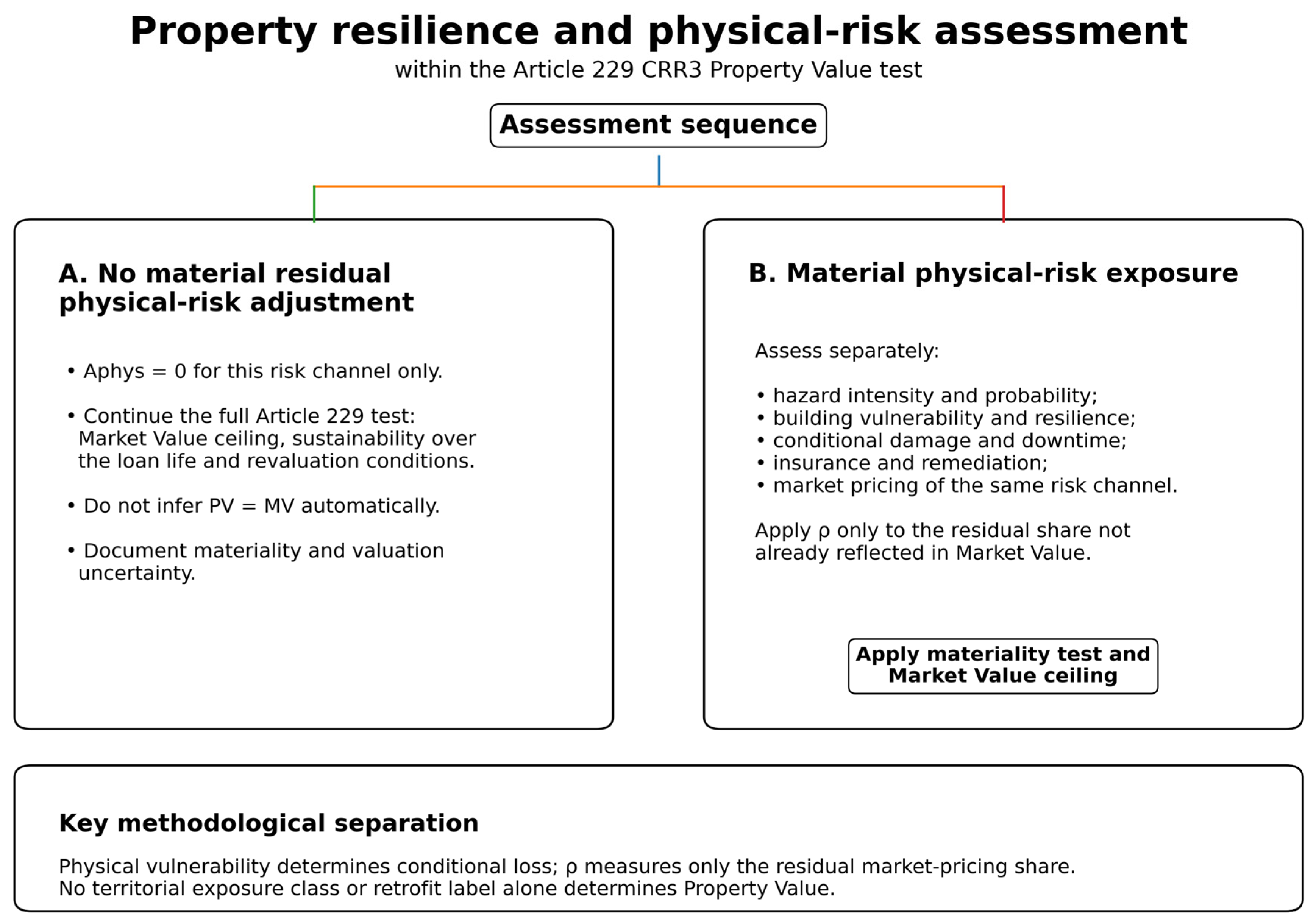
Physical risks relevant to real-estate value are heterogeneous. Climate-related physical risks include acute events and chronic changes; geophysical hazards such as earthquakes and volcanic events are natural physical risks but are not climate risks. Other environmental or nature-related risks may also be relevant where they have a demonstrable value channel. These risks may affect value through expected physical damage, interruption of use and downtime (For a building, “downtime” means the period between a damaging event and the complete restoration of the conditions of usability and functionality existing before the event. It concerns not only collapse or severe structural damage, but also damage to non-structural components, building services and contents, which are often the main cause of prolonged unavailability. In summary, for buildings, the relationship with use value and therefore economic value concerns: Vulnerability (how much it is damaged); Downtime (how long it remains unusable); Resilience (how quickly it returns to operation). A “resilient” building is therefore not merely one that does not collapse, but one that maintains its function or rapidly restores it; loss of rental income, insurance terms, adaptation or protection costs, liquidity and required returns. Their effect is not uniform and depends on hazard intensity, asset-specific vulnerability, resilience, use, loan horizon, insurance, and the extent to which the market already prices the risk (“Risk” is the possibility that a natural phenomenon or a phenomenon induced by human activities may cause harmful effects on the population, residential and productive settlements and infrastructure within a specific area over a given period. Risk may therefore be expressed as R = P × V × E, where P = hazard (the probability that a phenomenon of a given intensity will occur within a given period in a given area); V = vulnerability (the propensity of an element to suffer damage as a result of the stresses induced by an event of a given intensity); and E = exposure or value exposed (the number of units or value of each element at risk present in a given area). Figure 1 therefore presents a continuous residual-risk assessment rather than a binary exposed/not-exposed rule.

3.2. Structure of the Valuation Process

Where physical-risk information is materially relevant to the collateral, the proposed analytical process is structured into five sequential and interrelated stages:
  • Estimate market value (MV) at the valuation date using standard valuation approaches: the market comparison approach (MCA), income approach (direct capitalization or discounted cash-flow capitalization), and/or cost approach, depending on the type of property. Forecasting prices or rents over the long or very long term on the basis of real-estate market cycles is highly uncertain; indeed, as previously recalled in an ECB Supervision Newsletter, “there are currently no models that can reliably predict the future values of a specific property”.
  • Assess the sustainability of value over the life of the loan: using freely accessible public sources, assess the relationship between exogenous (extrinsic) variables and the asset’s resilience characteristics in order to determine whether current value already incorporates possible future risks; identify residual risk not incorporated into market prices.
  • Map and quantify the physical-risk profile: assess potential exposure using official European and national datasets selected according to the level of granularity required (e.g., WISE/Floods Directive and JRC/DRMKC at EU level; IdroGEO/ISPRA, INGV and the Department of Civil Protection for Italy).
  • Determine a possible environmental and physical-risk adjustment (Aphys): estimate only the material residual component not already priced by the market, using documented hazard probabilities, vulnerability information, effective insurance terms, property-level loss of use, non-overlapping restoration costs and a consistent discounting convention.
  • Determine PV and document the analysis: apply Equation (1) for the general/initial representation and the additional Article 229(1)(e) ceiling for revaluations as set out in Equation (2), and document the evidence, assumptions, uncertainty, sensitivity and any residual adjustments using appropriate European and national sources, energy-performance data and, where relevant, insurance information.

3.3. The Aphys Formula for Physical-Risk Adjustments

For event-based physical risks, this paper proposes the following first-order analytical formulation. It is designed to make the economic components of a possible residual adjustment explicit and auditable; it is not a complete probabilistic catastrophe-loss model, and it is not prescribed by CRR3, EBA or the ECB:
A p h y s = e = 1 m t = 1 n P r ( e , t ) · ρ ( e , t ) · D u n i n s ( e , t ) + L u s e ( e , t ) + C r e m ( e , t ) 1 + r p t
where:
  • Aphys = present value of the expected residual property-level loss attributable to physical, climate-related and environmental risks not incorporated into market value;
  • Pr(e,t) = probability of event e in period t under the selected hazard information and, where relevant, the selected forward-looking scenario; event intensity and asset vulnerability should be reflected in the conditional loss estimate or an underlying vulnerability function;
  • Physical vulnerability is conceptually upstream of the residual-pricing coefficient. For each event, the conditional damage component may be represented schematically as D(e,t) = f[I(e,t), Vbuilding, Rbuilding], where I(e,t) denotes event intensity, Vbuilding physical vulnerability, and Rbuilding resilience or mitigation. A retrofit or physical improvement should therefore affect Vbuilding/Rbuilding and the resulting conditional damage, downtime, or remediation assumptions. It should change ρ only where separate market evidence also demonstrates that the proportion of the remaining economic effect already incorporated in market value has changed.
  • Dunins(e,t) = physical damage to the property conditional on event e, measured through structural and non-structural repair/replacement costs required to restore damaged components, net of insurance recoveries that can reasonably be relied upon after deductibles, limits and exclusions, and excluding every item separately included in Crem;
  • Luse(e,t) = property-level economic loss from temporary unavailability, reduced habitability, lost rent or impaired use; borrower operating losses unrelated to the property’s own value are excluded;
  • Crem(e,t) = incremental post-event remediation or ancillary restoration cost not already included in Dunins, such as debris removal, temporary protection, environmental remediation or separately evidenced regulatory upgrading. Planned ex-ante adaptation expenditure is not probability-weighted as a contingent loss and should instead be treated separately as capex or another explicit adjustment where material and not already reflected in MV;
  • For each event-time pair, the economic content of Dunins and Crem must be mutually exclusive: Dunins(e,t) ∩ Crem(e,t) = ∅. The valuation file should reconcile the two buckets line by line. Repair or reinstatement of damaged structural and non-structural components belongs to Dunins; only ancillary or incremental post-event items not embedded in those repair estimates belong to Crem. This is an economic, not merely terminological, separation.
  • rp = discount rate used for expected residual losses, specified consistently on a nominal or real basis with the underlying loss estimates. It must not embed a risk premium for a risk already captured in event probabilities or expected losses;
  • m = total number of physical, climate-related and environmental event types considered for the purpose of the analysis;
  • n = loan term (or prudential analysis horizon).
The coefficient ρ(e,t), with 0 ≤ ρ(e,t) ≤ 1, represents the share of the relevant economic risk that remains unpriced in market value. It must not be selected at discretion. The proposed estimation hierarchy is: (i) define risk-homogeneous comparables by location, hazard, building type, vulnerability/resilience and relevant insurance characteristics; (ii) test whether transaction prices, rents, capitalization rates or other market evidence already reflect the risk, using matched-sales, repeat-sales, hedonic/spatial methods or other empirically appropriate designs where data permit; (iii) set ρ = 0 only where the relevant risk is demonstrably fully reflected, estimate 0 < ρ < 1 only where evidence supports partial pricing, and use ρ = 1 only where credible evidence supports the conclusion that the component is unpriced; and (iv) where evidence is insufficient, do not infer an arbitrary point estimate—report the data limitation and test a documented range in sensitivity analysis. This procedure makes ρ an empirically calibratable parameter rather than a free haircut coefficient. When partial pricing is evidenced, and the market-implied effect and the economic-loss benchmark can be expressed on the same present-value basis, an operational mapping may be written as ρ = max{0, min [1, 1 − Mpriced/Ggross]}, where Mpriced is the capitalized market effect attributable to the same risk channel, and Ggross is the present value of the corresponding gross expected property-level economic loss before the residual-pricing adjustment. Mpriced may be estimated from matched sales, hedonic/spatial coefficients, repeat-sales evidence, rent or capitalization-rate differentials, or evidence from a sufficiently comparable market, after controlling relevant confounders. The numerator and denominator must refer to the same hazard, property characteristics, time horizon, and economic-loss channel. Where either quantity is estimated as an interval, ρ should likewise be reported as a range; weak or non-comparable evidence should not be converted into a point estimate. This mapping is a proposed operational aid, not an empirically calibrated universal formula.
The Aphys formulation is primarily suited to event-based environmental, acute physical risks and geophysical events that can be represented through event probability and conditional loss. Chronic climate risks—such as gradual sea-level rise, chronic heat, drought or water scarcity—should not be forced into a single-event probability where that representation is inappropriate. Their value effects should instead be modeled through scenario-consistent changes in cash flows, operating costs, marketability, terminal value, or other empirically supported channels. Where multiple hazards overlap or are correlated, joint or conditional probabilities and vulnerability functions should be used where material; simple additivity is defensible only after overlap and repeated-loss effects have been controlled.
The formulation is designed to make the economic drivers of any prudential adjustment explicit and verifiable. It does not imply that every physical exposure should lead to a deduction from market value: an adjustment is justified only where the risk is materially relevant to the sustainability of value and is not already adequately incorporated into current prices.
The Aphys formulation may be informed by granular forward-looking hazard data and vulnerability functions linking event intensity to asset-specific damage. Its simplifying assumptions—including additivity, treatment of hazard dependence, insurance reliability, vulnerability, downtime and discounting—must be stated for each application. Results should be subjected to sensitivity analysis over the principal uncertain inputs, including ρ, event probabilities or scenario paths, vulnerability/damage assumptions, insurance recoveries, downtime and rp. The formulation remains a methodological proposal by the author and requires empirical calibration and external validation; it must not be interpreted as a source of standardized haircuts.
For example, at the European level, for the purpose of a simplified and more standardized screening of seismic damage, the European Macroseismic Scale 1998 (EMS-98) [31] may also be used. It is the first intensity scale accompanied by illustrations, in which the drawings and photographic examples in Section 5 facilitate field comparison with actually damaged structures. For damage classification, the scale distinguishes masonry and reinforced-concrete buildings and five grades (D1–D5), from negligible/slight damage to destruction; its use does not replace engineering analyses of hazard, vulnerability and fragility where required.
Although Aphys is labeled as an environmental and physical-risk adjustment, reflecting its primary purpose of quantifying residual physical-risk losses, its additive structure across event types and time periods is modular and can accommodate multiple hazards as well as additional measurable property-level loss channels. Social or Governance variables should not, however, be collapsed mechanically into Aphys. They may affect Aphys only where there is a documented causal link to one of its physical-risk inputs—for example by modifying vulnerability, property-level loss of use, remediation or compliance costs, insurance effectiveness, or another measurable consequence of a physical event. Otherwise, their value effects should be reflected separately through market evidence, cash flows, capex/opex, liquidity, legal/compliance costs or another expressly identified adjustment. This preserves the breadth of the ESG assessment recognized by the Italian Property Valuation Standard while maintaining analytical transparency and avoiding double counting [5].
Where scenario analysis is used for non-stationary climate risks, the selected pathway, time horizon, downscaling source, and treatment of model uncertainty should be documented. In line with the EBA Guidelines, scenario analysis informs the inputs to the valuation framework; it does not translate supervisory climate scenarios into automatic property haircuts [32].
Table 2 sets out the evidence chain expected in a real application. The numerical values used in Cases A-C remain constructed scenario assumptions; the table specifies how each input would instead be sourced, estimated, expressed, assigned an uncertainty range, and subjected to appropriate professional responsibility and control in an empirical valuation. The indication of the professional roles involved is, in any event, illustrative, since it must necessarily be aligned, and where necessary redefined, with the professional regulatory frameworks applicable in the different jurisdictions. Table 2 summarizes the principal Aphys inputs, the supporting empirical evidence, and the controls adopted to avoid double counting.

3.4. Estimating PV for Income-Producing Properties

For income-producing properties, MVRA may be represented by discounting property-level cash flows after distinct and non-overlapping physical-risk adjustments:
P V I P R E   =   min M V ,   t   =   1 n N O I t   -   E L t   -   C a p e x t   -   E x t r a O p e x t 1   +   r   +   Δ r t   +   T V n R A 1   +   r   +   Δ r n
where:
  • NOIt is the expected net operating income in period t, based on market-supported and prudently normalized assumptions and excluding unsupported expectations of future price or rent increases;
  • ELt is the expected loss from physical damage and/or interruption of use;
  • Capext comprises planned adaptation or protection expenditure attributable to the property and not already reflected in MV or another cash-flow item;
  • ExtraOpext comprises additional insurance and maintenance costs;
  • r is the market discount rate, used on a nominal or real basis consistently with the cash flows;
  • Δr is an additional premium only for residual risk components not already incorporated in ELt, Capext, ExtraOpext, terminal value or the base market discount rate;
  • TV n RA is the risk-adjusted terminal value at the end of the prudential analysis horizon. Continuing physical risk must be reflected through one, and only one, non-overlapping channel—for example, a risk-adjusted terminal NOI, a separately supported exit capitalization rate, or expected post-horizon capex/opex. It must not disappear mechanically after year n, and the chosen channel must be reconciled with ELt, Capext, ExtraOpext and Δr. The terminal assumptions must remain market-supportable and must not introduce speculative appreciation excluded by Article 229; assumptions on rent growth, inflation and exit capitalization should be internally consistent and should normalize rather than extrapolate short-term market-cycle peaks.
  • n = loan term (or prudential analysis horizon).
To avoid double counting, the preferred allocation is to reflect a quantifiable risk through the cash-flow item to which it directly relates; Δr should be used only for a distinct residual risk not captured elsewhere. ELt, Capext, ExtraOpext, Δr and TV n RA must therefore be reconciled explicitly. Inflation, taxation and other model conventions must be applied consistently with the chosen nominal/real basis. The parameterization will differ across office, retail, industrial, logistics and other sectors because lease structures, insurance, market liquidity and vulnerability channels differ; coefficients should not be transferred across sectors without validation.
A capitalization rate k and a discount rate r are conceptually distinct. A capitalization rate converts a stabilized one-period income into value and embeds assumptions regarding growth, depreciation and risk; a discount rate prices multi-period cash flows. The same numerical value should therefore be used only where an explicit cash-flow convention makes them consistent—for example, a zero-growth level-perpetuity illustration with otherwise aligned assumptions. In empirical applications, k and r should be estimated and justified separately unless such a convention is demonstrated.

3.5. Estimating PV for Residential (Non-Income-Producing) Properties

For non-income-producing residential properties, the notation is standardized as follows: PVR is the lower of current residential market value (MVR) and the residential risk-adjusted analytical value (MVRA,R), subject, on revaluation, to the additional Article 229(1)(e) ceiling:
PVR = min [MVR, MVRA,R]
The residential risk-adjusted market value (MVRA,R) is obtained as follows:
MVRA,R = MVR − Aphys − Aenergy − Alegal,residual − Aliquidity
where:
  • Aenergy = residual value effect attributable to energy performance only where it is material and not already reflected in MVR;
  • Alegal,residual = any remediable legal/planning/cadastral cost not already reflected in MVR. This is a baseline property/legal valuation issue, not an ESG category (Alegal (building, planning and cadastral compliance) is intended to identify non-compliances which, where remediable, would entail regularization costs or costs to restore the property to its compliant condition).
  • Aliquidity = residual marketability effect in a high-risk context only where it is empirically supported and not already incorporated into comparable prices. Planned ex-ante adaptation expenditure, where relevant, is treated separately rather than probability weighted as contingent loss.
The Aenergy, Alegal,residual and Aliquidity components are analytical variables of this framework, not adjustment categories prescribed by CRR3. Each is used only where the effect is material, adequately evidenced, and not already incorporated into market value. In a strictly subtractive residential implementation, the min operator is mathematically redundant whenever MVRA,R can only be below MVR; it is retained in Equation (5) to make the Article 229 market value ceiling explicit and to keep notation aligned with the general framework.

3.6. Avoiding Double Counting

A methodologically critical issue is the risk of double counting. If the comparables used to estimate MV are homogeneous with respect to the subject property’s material risks and those risks are already reflected in market prices, automatically applying an additional haircut would result in an unjustified penalty. The Aphys adjustment should therefore address only: (i) residual risk not incorporated into current prices; and/or (ii) reasonably foreseeable future conditions over the life of the loan that are materially relevant but not yet priced by the market. Article 229 CRR3 establishes the prudential outcome to be achieved but does not prescribe a specific haircut formula; the distinction between generic approaches and more granular, forward-looking methodologies instead emerges from the supervisory practices described by the ECB.
Where the comparables used to estimate MV have a demonstrably homogeneous risk profile, observed prices may already incorporate all or part of the relevant risk discount; materially different risk profiles require comparability adjustments. The identification procedure should therefore document: the hazard and property characteristics used to define the comparable set; whether price, rent or capitalization-rate evidence shows full, partial or no pricing; the empirical method used to infer any residual share; and the resulting ρ range. This procedure is intended to make the no-double-counting conclusion replicable rather than dependent on an unsupported expert assertion.
Because Article 229 does not define a universal numerical threshold for ‘significantly above’, materiality is operationalized in Equation (1) as a decision gate rather than as an automatic haircut. ΔV = MV − MVRA is compared with a documented mandate- or institution-specific criterion τ and with credible valuation/model uncertainty. If ΔV ≤ τ, or the difference lies within documented valuation uncertainty, PV remains MV under the proposed operational rule. Only where ΔV > τ and the difference also exceeds the documented uncertainty allowance (or lies outside the corresponding uncertainty range) does the lower-of-MV-and-MVRA rule apply. τ may be expressed as an absolute amount, a percentage of MV, or another documented metric, provided that it is translated onto a basis comparable with ΔV; neither τ nor the uncertainty allowance U is a CRR3-prescribed threshold.

3.7. Illustrative Numerical Cases and Sensitivity Analysis

The following cases operationalize the framework using transparent illustrative inputs. Their purpose is to show how the residual-risk logic, no-double-counting rule, and Aphys formulation work in practice across different property types and hazards. The comparable data and residual-risk shares are scenario inputs constructed for the worked applications; they are not presented as an observed empirical sample. Accordingly, the cases provide an internal-consistency and computational-implementation illustration, while empirical calibration and external validation remain necessary.

3.7.1. Case A—Residential Property in a Hydraulic-Hazard Area (Emilia-Romagna)

Asset and context. The subject is an 85 m2 ground-floor apartment in a 1980s residential building in Emilia-Romagna. It is assumed to have no dedicated hydraulic-mitigation measures and to be located in an area classified as P2 in the competent hydraulic-hazard mapping. The loan horizon is 25 years. The EPC is class E, and no material planning or cadastral non-compliance is assumed. The P2 administrative/hazard class is not converted mechanically into an annual damage probability; the event probability used below is a separate scenario input.
Market value and priced location risk. MVR is estimated using the market comparison approach using three illustrative comparables. Two are in the same P2 micro-area and therefore provide evidence of the broad location-risk component already reflected in local prices; a third comparable outside the risk area is adjusted to the subject micro-area. The implied 17% location adjustment is constructed within the case and is not a generalizable empirical flood discount. Because the market value analysis already controls location risk and EPC characteristics, the base case does not apply a separate Aliquidity or Aenergy deduction: absent additional evidence, doing so would risk double counting. Table 3 presents the market comparison approach (MCA) and the resulting market value (MV) estimate for Case A.
Residual physical-risk adjustment. For the worked scenario, Prflood = 2.0% per year is assumed independently of the P2 label. Conditional property-level loss is EUR 18,000 of uninsured repair/replacement of damaged building components + EUR 3960 of property-level loss of use + EUR 8000 of ancillary post-event remediation (debris removal, drying/clean-up and temporary protection assumed in the scenario and excluded from the EUR 18,000 repair estimate) = EUR 29,960. The ground-floor position and absence of hydraulic mitigation affect the conditional-loss assumptions; independently, ρ = 40% is used as a residual market-pricing scenario assumption to represent partial market recognition of the same economic risk channel. It is not an empirical estimate and is varied separately in sensitivity analysis.
Sensitivity. The table varies event probability, residual-risk share, and the discount rate. The direction of the results is consistent with the framework: higher event probability or a larger residual unpriced share reduces PV, while a higher discount rate reduces the present value of a fixed expected-loss stream. The resulting MVRA,R remains an analytical intermediate; in the base-case decision example in Table 4, it becomes PV because ΔV exceeds both the illustrative τ and the uncertainty allowance. Sensitivity outputs remain conditional unless the same documented materiality test is applied to each scenario. Table 4 presents the residual expected loss and the resulting property value for Case A. Table 5 presents the sensitivity analysis for Case A.

3.7.2. Case B—Income-Producing Commercial Property in a High-Seismic-Hazard Area (Marche)

Asset and context. The subject is a 1200 m2 office/commercial building constructed in 1990 in a Marche municipality classified in Seismic Zone 1. The administrative zone signals high hazard but does not by itself determine site-specific seismic action or building damage probability; a real application would combine INGV/technical hazard inputs with the building vulnerability model. The worked case assumes an illustrative vulnerability/risk class D, no complete structural retrofit, no earthquake insurance, a 15-year loan, annual gross rent of EUR 96,000, 5% vacancy, and EUR 18,000 annual operating costs, giving a current NOI of EUR 73,200.
Market value. A market capitalization rate of 7.5% is assumed for comparable office properties in the same area. Because that market rate is derived from the same location, the broad seismic-zone component is treated as already priced. MV = 73,200/0.075 = EUR 976,000 (rounded).
Residual-risk and cash-flow architecture. The worked scenario assumes a 2.0% annual probability of an event capable of producing material structural damage. Physical vulnerability is represented through the assumed conditional-loss vector, not through ρ. The scenario uses ρ = 60% solely as a residual market-pricing assumption: it represents the share of the resulting property-level economic effects assumed not to be incorporated in the market evidence underlying MV. Neither Prseismic nor ρ is inferred mechanically from Seismic Zone 1 or from retrofit status. Conditional loss is kept mutually exclusive across components: EUR 350,000 represents uninsured structural/non-structural repair and replacement; EUR 45,000 represents 180 days of effective rental-income loss after the stated 5% vacancy allowance [EUR 96,000 × (1 − 0.05) × 180/365, rounded]; and EUR 80,000 represents ancillary post-event remediation and temporary-protection items assumed not to be included in the EUR 350,000 repair estimate. The scenario assumes no earthquake insurance, no rent recovery under the lease during unusability, and no reduction of the baseline operating costs during downtime; if recoverable or avoidable operating costs, insurance proceeds, or different lease obligations applied, Luse and/or the other cash-flow inputs would need to be adjusted accordingly. No additional Δr is included in the base case because there is no separate empirical evidence for a residual investor-risk premium beyond the quantified cash-flow loss; Δr should be used only for a distinct, non-overlapping residual component. As shown in Table 6, Case B presents the expected residual property-level loss.
Capitalization and discounting convention.
The 7.5% market capitalization rate k is first used to derive MV from current stabilized NOI. A capitalization rate and a discount rate are conceptually distinct. For this constructed illustration only, the numerical discount rate r is also set at 7.5% under an explicit zero-growth, level-income/level-expected-loss convention, so that k = r when g = 0. The annual expected residual property level loss is EUR 5700. Continuing risk is not allowed to disappear after year 15: the terminal value is calculated from a risk-adjusted terminal NOI of EUR 73,200 − EUR 5700 = EUR 67,500, using the same 7.5% exit capitalization rate and no additional overlapping risk premium. Under these assumptions, the 15-year DCF plus risk-adjusted terminal value is equivalent to capitalizing the level risk-adjusted NOI, giving MVRA ≈ EUR 900,000 and a continuing residual adjustment of EUR 76,000. In an actual valuation, k and r would be estimated separately unless the same convention is empirically justified, and the terminal-risk channel would be documented explicitly. Table 7 reports the property value determination for Case B. Table 8 presents the sensitivity analysis for Case B.
The sensitivity analysis varies the residual market-pricing assumption (ρ) and physical-vulnerability/conditional-loss assumptions separately. An illustrative post-retrofit effect is represented through a lower conditional loss with ρ held constant unless independent market evidence supports a change in the proportion of risk already priced. A separate discount-rate or residual premium change would likewise require distinct evidence and must not duplicate expected losses or terminal-value assumptions.
In this respect, the treatment of terminal value deserves specific attention in a prudential DCF framework. D’Amato and Bambagioni [33] discuss alternative approaches to the determination of exit value and emphasize the need to relate terminal-value assumptions to market conditions and to the long-term sustainability of cash flows.
More broadly, recent U.S. professional valuation literature supports a market-informed treatment of physical risk. Robinson [34] argues that physical weather risk may be relevant to valuation where it is financially material and evidenced in market behavior, with potential transmission through operating and insurance costs, net operating income, capitalization and discount rates, resilience-related capital expenditure, liquidity and marketability. Importantly, the existence of physical exposure does not by itself justify a uniform adjustment; the valuation response should depend on whether and how market participants incorporate the relevant risk into pricing and investment decisions. This is consistent with the separation adopted here between physical vulnerability, market pricing and residual unpriced risk.

3.7.3. Case C—Residential Property with Partial Seismic Improvement (Messina, Sicily)

Asset and context. The subject is a 95 m2 second-floor apartment in a 1960s residential building in Messina, a municipality classified in Seismic Zone 1. The building is assumed to have undergone a partial seismic improvement in 2015, represented for the worked case by an illustrative class C vulnerability/risk profile compared with an unretrofitted class E profile. The loan horizon is 20 years, the EPC is D, no material planning or cadastral non-compliance is assumed, and hydrogeological risk in the micro-area is treated as immaterial. The administrative seismic zone is used for screening only; the scenario event probability is not inferred mechanically from the zone classification.
Market value and resilience pricing. Three illustrative comparables are used to isolate a resilience differential. Comp. 1 is aligned with the subject’s partial seismic improvement; Comp. 2 requires floor, condition, and EPC adjustments; Comp. 3 has otherwise similar characteristics but an unretrofitted class E profile and is adjusted upward to the subject’s class C profile. The 9.8% differential between Comp. 1 and Comp. 3 is an internal feature of the constructed case dataset, not an empirical estimate for the Messina market. It is used to demonstrate how resilience that is already priced in market value must not be deducted again through Aphys. The market comparison approach and the related resilience adjustment for Case C are reported in Table 9.
Residual physical-risk adjustment. The worked scenario assumes Prseismic = 2.2% per year for an event capable of producing material building damage. The physical effect of the partial improvement is represented in the conditional-loss assumptions and in the resilience adjustment used in the comparable analysis; it is not used to determine ρ. Independently, ρ = 35% is adopted as a residual market-pricing scenario assumption representing partial pricing of the same economic risk channel. Neither Prseismic nor ρ is derived mechanically from the administrative zone or retrofit status. Conditional loss comprises EUR 95,000 of uninsured repair/replacement of damaged building components, EUR 3045 of property-level loss of use, and EUR 30,000 of ancillary post-event remediation/temporary-protection costs that are assumed not to be embedded in the EUR 95,000 repair estimate. Table 10 presents the residual expected loss and the resulting property value for Case C.
As in Case A, no separate Aenergy or Aliquidity is deducted in the base case because the comparable analysis already controls EPC and the local risk context. A further deduction would require separate evidence of a residual value effect not already reflected in market value. In the sensitivity analysis, the effect of a fuller retrofit is therefore represented by a lower conditional-loss assumption while ρ is held at 35%; ρ changes only in the separate market-pricing sensitivity. Table 11 presents the sensitivity analysis for Case C.

3.7.4. Cross-Case Comparison

The three applications generate different analytical adjustments because the property type, physical vulnerability/conditional loss, residual unpriced-market share, horizon, and discounting assumptions differ. Physical vulnerability and ρ are varied separately. The results should not be read as market-wide haircut benchmarks or empirical building-performance estimates. Their role is to illustrate the computational behavior of the framework and to show explicitly how no-double-counting and materiality choices affect the result. A cross-case comparison of the base scenarios is presented in Table 12.
Across the constructed base scenarios, the difference between MV and MVRA ranges from approximately 2.6% to 8.8%. These are outputs of the scenario assumptions, not empirically calibrated prudential ranges. In Case A, the 2.6% analytical difference is not treated as an automatic CRR3 deduction: Table 4 provides a purely illustrative application of Equation (1), using τ = 2.0% of MV and an uncertainty allowance U = 1.5% of MV. Under those scenario assumptions, ΔV exceeds both MV and MVRA,R becomes the illustrative PV; different documented mandate- or institution-specific criteria or uncertainty ranges could instead result in PV remaining equal to MV. For CRR purposes, the relevant effect must ultimately be assessed through the applicable ETV definition and exposure treatment rather than through the illustrative LTV ratios alone.


4. Discussion

4.1. From Market Value to Property Value

The methodological framework developed in this paper has implications beyond the valuation of an individual property. Under Article 229 CRR3, physical-risk exposure does not mechanically require a downward adjustment to market value; the relevant question is whether current market value may be significantly above the value sustainable over the life of the loan after the full prudently conservative test has been applied. CRR3 does not prescribe a numerical threshold for “significantly above”. Accordingly, this framework does not invent one: any adjustment should be supported by a documented materiality assessment and should be distinguishable from ordinary valuation/model uncertainty rather than triggered by immaterial model noise. Equation (1) operationalizes this by retaining MV where ΔV is immaterial or lies within documented uncertainty and applying the lower value only where the difference is supported as material. This decision rule is proposed by the author and is not a CRR3 numerical threshold. Case A provides a worked illustration of this gate using a hypothetical τ and uncertainty allowance; these inputs demonstrate the decision mechanics only and do not imply a universal CRR3 threshold.
This distinction requires the valuation to be sufficiently granular to separate exposure to the hazard from the asset’s actual vulnerability and from residual economic risk. At the same time, the prudential adjustment must not duplicate risks already reflected in observed prices: the interaction between market value, exposure to physical risks, property resilience, insurance coverage and market pricing therefore becomes central to the determination of property value.
Within this proposed framework, property value is treated as the outcome of a prudential test applied to current market evidence rather than as an autonomous value basis constructed in opposition to the market. This is one possible implementation pathway among the approaches described by International Valuation Standards (IVS) [3]. The contribution is to make explicit the logical sequence from risk information, through its potential capitalization into market value, to the residual component capable of affecting sustainability over the life of the loan.

4.2. Residual Risk, Vulnerability and Resilience

Mapping residual risk is the discriminating factor: a granular analysis showing low residual exposure helps avoid unjustified haircuts. Exposure to physical risk does not automatically imply a loss in value; what matters is the combination of hazard, asset-specific vulnerability, resilience and adaptation, use, insurance coverage and potential downtime, together with the extent to which these factors are already reflected in market prices.
Resilience improvements may reduce physical vulnerability, conditional damage, downtime or remediation costs. Separately, if market evidence shows that improved resilience is more fully capitalized into prices, rents or capitalization rates, the residual-pricing coefficient ρ may also change. The two effects must be evidenced separately and should not be inferred from one another. The magnitude of either benefit cannot be assumed ex ante or automatically equated with the cost of the intervention: it must be estimated and documented.
The sequence hazard → vulnerability → damage → downtime → economic consequence constitutes, within the framework, the principal transmission channel from physical risk to the sustainability of value. This sequence makes it possible to distinguish simple territorial risk classification from the actual vulnerability of the property and, above all, from the economic effect relevant to valuation.
U.S. post-disaster appraisal literature and professional guidance provide a complementary perspective on this need for market-specific judgment. Nguyen [35] develops a post-disaster appraisal framework in which value effects, risk perception, insurance dynamics, regulatory constraints and distorted comparables are integrated into USPAP-compliant appraisal reasoning. Appraisal Institute Guide Note 10 likewise addresses the development of market value opinions after disasters, emphasizing the instability of affected markets and the need to assess whether observed transactions satisfy the conditions underlying market value [36]. These sources are jurisdiction-specific and are not imported into the CRR3 framework as prescriptive rules; they are cited as comparative professional evidence supporting transparent, market-grounded analysis under physical-risk conditions.
Related U.S. appraisal guidance also illustrates how other environmental factors may be decomposed for valuation purposes. Appraisal Institute Guide Note 6, which expressly addresses the application of USPAP to property affected or potentially affected by environmental contamination and draws on USPAP Advisory Opinion 9, distinguishes the impaired value of a contaminated property from its hypothetical unimpaired value and separates remediation-cost effects, use effects, and environmental risk/stigma [37]. This distinction is conceptually consistent with the non-duplicative treatment of environmental effects adopted in the present framework.

4.3. Implications for ETV/LTV and Risk-Weighted Exposure Amounts

Determining a property value below market value increases the ratio between the exposure and the value of the collateral. For strictly prudential CRR3 purposes, however, reference must be made to the exposure-to-value ratio (ETV) and to the treatment applicable to the specific exposure. Articles 124–126 of the CRR provide differentiated mechanisms and risk weights depending, among other factors, on whether the property is residential or commercial, whether the exposure is classified as IPRE or non-IPRE, and the applicable method; accordingly, there is no universal 80% threshold applicable to all exposures. A change in property value may affect ETV and, depending on the relevant bucket and prudential treatment, risk-weighted exposure amounts. (The exposure-to-value ratio (ETV) is the prudential ratio between the gross exposure amount and the property value. Article 124(6) CRR3 provides the following definition: “For the purposes of Article 125(2) and Article 126(2), the exposure-to-value (“ETV”) ratio shall be calculated by dividing the gross exposure amount by the property value […].” Accordingly: ETV = Gross Exposure Amount/property value. The denominator, property value, is not simply the market value of the property: the CRR defines it as the value of residential or commercial immovable property determined in accordance with Article 229(1). This is particularly relevant for the purposes of this paper, since the prudential determination of property value directly affects the ETV; the numerator is also more technical than the simple “loan amount”. Article 124(6) provides that the gross exposure amount includes the carrying amount of the exposure secured by the immovable property plus any undrawn but committed amount which, once drawn, would increase the exposure secured by the immovable property. The calculation is made gross, inter alia, of specific credit-risk adjustments and, as a general rule, without taking credit protection into account, subject to the specific exceptions provided by the regulation).
The worked applications illustrate this mechanism without suggesting a universal threshold. In the base-case scenarios, the illustrative LTV increases by approximately 1.6 percentage points in Case A, 6.1 percentage points in Case B and 6.8 percentage points in Case C when the denominator changes from MV to PV. The prudential consequence, if any, depends on the applicable ETV bucket, exposure classification and CRR treatment; the case-study LTV figures are therefore explanatory rather than substitutes for the regulatory ETV calculation.

4.4. Insurance Coverage and the Physical-Risk Protection Gap

Integration of insurance coverage into the valuation process requires more than a binary insured/uninsured indicator. Relevant inputs include deductibles, policy limits, exclusions, coverage of the identified hazard, expected renewal availability, insurer/guarantor reliability and, where material, payment timing; public compensation should be recognized only where there is a sufficiently reliable legal and empirical basis. In Aphys, Dunins is therefore net of recoveries that can reasonably be relied upon, while insurance premiums or other recurring costs belong in property cash flows. Where coverage is unavailable and expected physical-risk costs are not already incorporated into collateral value, the ECB describes prudential responses such as lower ETV/LTV limits or other credit thresholds [8].

4.5. Data Infrastructure, Monitoring and Valuation Governance

The ECB Good Practices for Climate and Nature Risk Management—Observations from the ECB’s Five-Year Climate and Nature Risk Programme (2020–25) [8] as non-binding illustrative examples, show possible operational approaches to integrating climate and nature risks into collateral management. The implications set out below must be read within the framework of CRR/CRD requirements, applicable EBA Guidelines and internal procedures proportionate to the bank’s risk profile.
  • Use of forward-looking approaches: the ECB describes both simpler approaches, including generic haircuts or proxies, and more granular forward-looking practices that quantify event probabilities and expected losses by location and asset characteristics. The Aphys framework proposed in this paper is methodologically aligned with the latter approach, without thereby conferring any regulatory or binding status on the formula.
  • Updating collateral value (Article 208 CRR): monitoring must capture information that may indicate a significant decline in value and the other triggers provided for by the applicable framework and internal procedures. Material physical events, updates to risk maps or changes in asset characteristics may constitute indicators requiring review; not every update to a classification should be treated as an automatic regulatory trigger in the absence of a materiality assessment.
  • Data infrastructure and the mandate of independent valuers: the ECB Good Practices demonstrate the usefulness of instructions enabling the collection and documentation of granular physical-risk data (geolocation, hazard, energy performance, insurance coverage, construction and seismic characteristics), to the extent that such information is materially relevant and available.

Documentation Requirements and Official Sources

Article 229 CRR3 requires the value to be documented in a transparent and clear manner; within the proposed framework, any adjustments attributable to physical risks should therefore be supported by verifiable documentation, consistent with the applicable EBA Guidelines. There are potentially numerous freely accessible official sources that may be consulted and cited in the valuation file. At EU level, relevant publicly accessible sources include:
  • the JRC Disaster Risk Management Knowledge Centre Risk Data Hub for multi-hazard screening;
  • WISE and the flood hazard and risk maps reported by Member States under Directive 2007/60/EC for flood risk (WISE: Available online: https://water.europa.eu/freshwater (accessed on 27 June 2026));
  • the JRC/ESDAC European Landslide Susceptibility Map (ELSUS) for landslide susceptibility;
  • Copernicus EFFIS for wildfire risk;
  • the European Drought Observatory for drought-related hazards; and
  • Copernicus Climate Change Service and Climate-ADAPT datasets for climate-related and coastal hazards. These pan-European sources should be complemented, where available, by the more granular hazard maps and technical datasets produced by the competent national and regional authorities (Copernicus Climate Change Service (C3S): https://climate.copernicus.eu/; Climate-ADAPT (EEA/European Commission): https://climate-adapt.eea.europa.eu/).
The classification provided by a hazard map should not, by itself, be interpreted as the probability of economic damage to the collateral. The latter requires the combination of hazard intensity and probability with the asset-specific vulnerability, exposure, resilience and mitigation characteristics.
These are supplemented by national official sources and, where appropriate, additional specialized databases. In Italy, for example, the following are available online: IdroGEO/ISPRA (hydrogeological risk) [38]; INGV (National Institute of Geophysics and Volcanology) for seismic and volcanic hazard; and the European Macroseismic Scale (EMS) [31]; the Department of Civil Protection (municipal seismic classification); SNPA (supplementary environmental data); and SIAPE/ENEA for APE/EPC data. Depending on the risk analyzed, event-history data may also be drawn from ISPRA, hydrological yearbooks, and specialized databases such as EM-DAT; insurance data (premiums, deductibles, and exclusions) provide a complementary source for economic quantification (The EPBD (Energy Performance of Buildings Directive) defines the parameters of the EPC (Energy Performance Certificate). From 1 November 2025, ENEA introduced a functionality for preparing Attestati di Prestazione Energetica (APE); through a dedicated web application (API) connected to the national SIAPE system (Sistema Informativo sugli Attestati di Prestazione Energetica), it is possible to include in certificates a parameter relating to the energy performance of similar existing buildings).
These components are already identified in the Codice delle Valutazioni Immobiliari (Italian Property Valuation Standard), Chapter 12 (valuation for mortgage lending purposes) and Chapter 23 (Real Estate Risk Assessment and ESG Rating).

4.6. Methodological Limitations, Compliance Implications and Research Agenda

Failure to consider material physical risks may give rise to compliance issues under the applicable prudential requirements, as well as risk-management deficiencies that may be examined in supervisory dialogue. It would, however, be incorrect to state that failure to adopt a specific ECB Good Practice is in itself a compliance breach: the Good Practices are not binding, and a bank may comply through different solutions suited to its risk profile and business model.
The EBA Guidelines (EBA/GL/2025/01) apply from 11 January 2026, with application by 11 January 2027 at the latest for small and non-complex institutions. They require arrangements to identify, measure, manage and monitor material ESG risks. The adequacy of collateral-related processes must be assessed in light of the overall prudential framework and in accordance with the principle of proportionality.
The principal limitation of the framework is that the three applications introduced in this revision are constructed numerical worked cases rather than an observed-data validation sample. They materially strengthen the applied component by showing how market value, residual-risk identification, Aphys, income-based adjustments, property value, and sensitivity analysis interact in residential and commercial settings. However, the comparable data and residual-risk shares used in the cases are scenario inputs and should not be interpreted as empirically estimated coefficients. Determining ρ(e,t) and the other Aphys inputs for real-world use requires observed transaction, hazard-intensity, building-vulnerability, insurance, loss, restoration-cost and downtime data. The cases therefore test internal coherence and computational implementation; they do not establish external statistical validity.
A second limitation concerns transferability across Member States, markets, property sectors and building types. The CRR3 regulatory logic is EU-wide, but hazard data, construction standards, insurance penetration, disclosure, market liquidity, investor behavior and valuation practice differ materially. The Italian Property Valuation Standard and Italian public datasets used here are illustrative implementation references. The scenario parameters used in the three worked cases are case-specific and should not be transferred to another country, market or sector without observed-data calibration and external validation.
Further research should therefore extend the three worked applications to observed samples of residential and commercial properties in different geographical areas, empirically assess the extent to which comparables incorporate physical risks, estimate ρ and the other Aphys parameters using the mapping process described in Section 3.3 together with matched-sales, repeat-sales, hedonic/spatial, insurance-claims or other appropriate data, and compare model outputs with realized market and loss evidence. Only at a later stage should consideration be given to extending the framework to transition risks, agro-industrial properties and broader nature-related risks, including biodiversity and environmental degradation.

5. Conclusions

For banking institutions, PV requires integration among credit functions, ESG risk assessment, collateral management and independent valuers.
Loan origination should include a minimum set of property-specific information, while monitoring should provide for review triggers based on changes in risk, updates to maps and data, loss events, regulatory changes, insurance changes and movements in the local market.
For valuers, CRR3 confirms the requirement of independence and professional qualifications; within the proposed framework, valuation also requires adequate information to map materially relevant risks and determine the prudential value of the property used as collateral. Adjustments should not be expressed as unsupported standard percentages, but as estimates linked to economic drivers: expected loss in relation to event probability (taking the term of the mortgage into account), mitigation cost, risk premium, reduced marketability, changes in expected cash flows or terminal value. Where evidence is insufficient, the valuer should state the information limitations and explain any decision not to apply a specific adjustment.
To this end, this paper proposes a conceptual, methodological and numerical framework for determining property value under Article 229 CRR3, focusing on property resilience, energy efficiency and materially relevant physical risks. The framework takes the IVS and European valuation guidance into account [4,6,7], uses the Codice delle Valutazioni Immobiliari as an illustrative national methodological reference [5], and compares the proposed process with the non-binding ECB Good Practices published in May 2026. It does not claim clause-by-clause compliance of the equations with every professional standard.
Methodologically, the new framework does not require the automatic replacement of market value with a separate basis of value or the generalized application of standardized haircuts. Within the proposed framework, these criteria are translated into a test of whether, after mapping the risks to which the building is exposed and considering its resilience and energy-efficiency characteristics, current market value may be significantly above the value sustainable over the life of the loan, taking into account the asset’s specific characteristics and materially relevant risks.
A central principle of the framework is no double counting. Exposure to a physical risk does not automatically equate to a loss in value: economic relevance depends on the combination of hazard, vulnerability, resilience, use, insurance coverage, potential downtime and the extent to which the risk is already incorporated into current prices. A prudential adjustment is therefore methodologically justified for the materially relevant component of risk that is not already reflected in market value, or that is attributable to reasonably foreseeable future conditions over the life of the loan.
The Aphys formulation provides one possible analytical representation of the residual event-based component, linking the potential adjustment to event probability, uninsured property damage, property-level loss of use, non-overlapping restoration costs, and, more generally, ESG risks, while allowing the loan horizon and asset-specific characteristics to be taken into account. It is a methodological proposal developed by the author and is not prescribed by CRR3, the EBA, or the ECB. The three worked cases illustrate how the formulation can be parameterized and subjected to sensitivity analysis; however, the scenario coefficients remain subject to empirical calibration and validation, and the results do not establish a systematic correlation between building performance and the resulting valuation adjustments.
Accordingly, the focus of the three numerical applications on physical risks should not be read as limiting the broader ESG assessment where other factors are material. The same valuation architecture can accommodate additional social, governance, or other ESG-related property-level variables through the appropriate valuation channel, provided that the economic transmission to value is evidenced, separately quantified where possible, and not already reflected in market value.
The original contribution of the paper is therefore: (i) to connect empirical evidence on physical-risk value channels with the prudential valuation question under CRR3; (ii) to formalize a market-capped and sustainability-tested representation that explicitly separates priced from residual unpriced risk; (iii) to provide an Aphys representation and decision procedure; and (iv) to illustrate the internal computational application of the framework through three numerical cases covering residential hydraulic risk, commercial seismic risk and residential seismic resilience, each accompanied by sensitivity analysis. Existing CRR3 requirements, EBA guidance, valuation standards and ECB good practices are treated as inputs and constraints rather than as elements claimed as original to the paper.
The three applications provide an initial numerical illustration and show that the outputs respond in the expected direction to changes in event probability, the residual unpriced-market share and physical vulnerability/conditional-loss assumptions when these mechanisms are varied separately. They do not constitute empirical calibration, external validation, or evidence of actual building performance. Observed data should next be used to test the extent to which physical risks are capitalized into market value and to calibrate the residual component by asset characteristics, building vulnerability and location. From this perspective, property value provides a bridge between property valuation and forward-looking prudential risk assessment: its purpose is not to detach collateral valuation from the market, but to test whether the market value observed today remains sustainable over the life of the loan.

Funding

This research received no external funding.

Institutional Review Board Statement

Not applicable.

Informed Consent Statement

Not applicable.

Data Availability Statement

No new empirical dataset was created or analyzed in this study. The numerical inputs used in the three worked cases are illustrative scenario data and are reported in the manuscript; observed-data calibration and external validation remain a subject for future research.

Acknowledgments

During the preparation of this manuscript, the author used OpenAI (GPT-5.6 Sol) for English-language translation and editorial formatting; nevertheless, the author reviewed and edited all outputs and takes full responsibility for the content of this publication.

Conflicts of Interest

The author declares no conflicts of interest.

Abbreviations

The following abbreviations are used in this manuscript:
AphysOverall adjustment for physical risks, including climate- and environment-related physical risks
Basel IIIThe international regulatory framework for banks
BCBSBasel Committee on Banking Supervision (hosted by the Bank for International Settlements (BIS), in Basel, CH)
CRR3Regulation (EU) 2024/1623 of the European Parliament and of the Council of 31 May 2024 amending Regulation (EU) No 575/2013 as regards requirements for credit risk, credit valuation adjustment risk, operational risk, market risk and the output floor (Capital Requirements Regulation)
CRD6Directive (EU) 2024/1619 of the European Parliament and of the Council of 31 May 2024 amending Directive 2013/36/EU as regards supervisory powers, sanctions, third-country branches, and environmental, social and governance risks.
EBAEuropean Banking Authority
ECBEuropean Central Bank
EMS-98European Macroseismic Scale
ESGEnvironmental, social and governance
ETVExposure-to-value ratio
IVSInternational Valuation Standards
IVSCInternational Valuation Standards Council
IPVSItalian Property Valuation Standard (Codice delle Valutazioni Immobiliari)
IPREIncome-producing real estate
LTVLoan-to-value ratio
MCAMarket comparison approach
MVMarket value
OECDOrganisation for Economic Co-operation and Development
PVProperty value
PrVPrudential value
MVRARisk-adjusted market value (analytical variable used in the proposed framework)
RWARisk-weighted assets

References

  1. European Parliament and Council of the European Union. Regulation (EU) 2024/1623 of 31 May 2024 amending Regulation (EU) No 575/2013 as regards requirements for credit risk, credit valuation adjustment risk, operational risk, market risk and the output floor. Off. J. Eur. Union 2024. Available online: https://eur-lex.europa.eu/eli/reg/2024/1623/oj/eng (accessed on 9 September 2026).
  2. European Parliament and Council of the European Union. Directive (EU) 2024/1619 of 31 May 2024 amending Directive 2013/36/EU as regards supervisory powers, sanctions, third-country branches, and environmental, social and governance risks. Off. J. Eur. Union 2024. Available online: https://eur-lex.europa.eu/legal-content/EN/TXT/PDF/?uri=OJ:L_202401619 (accessed on 9 September 2026).
  3. International Valuation Standards Council (IVSC). IVSC Statement Regarding Prudential Value for Real Estate; International Valuation Standards Council (IVSC): London, UK, 2025. [Google Scholar]
  4. International Valuation Standards Council (IVSC). International Valuation Standards; Effective 31 January 2025; IVSC: London, UK, 2025; ISBN 978-0-9931513-7-8. [Google Scholar]
  5. Bambagioni, G. Codice delle Valutazioni Immobiliari/Italian Property Valuation Standard, 6th ed.; Tecnoborsa SCpA: Rome, Italy, 2025. [Google Scholar]
  6. Royal Institution of Chartered Surveyors (RICS). ESG and Sustainability in Commercial Property Valuation, 4th ed.; Effective 30 April 2026; RICS: London, UK, 2026. [Google Scholar]
  7. TEGOVA. European Valuation Standards, 10th ed.; The European Group of Valuers’ Associations: Brussels, Belgium, 2025. [Google Scholar]
  8. European Central Bank (ECB). Good Practices for Climate and Nature Risk Management—Observations from the ECB’s Five-Year Climate and Nature Risk Programme (2020–25); ECB Banking Supervision: Frankfurt am Main, Germany, 2026; Available online: https://www.bankingsupervision.europa.eu/ecb/pub/pdf/ssm.thematicreviewcercompendiumgoodpractices052026.en.pdf (accessed on 9 September 2026).
  9. European Banking Authority (EBA). Guidelines on the Management of ESG Risks; EBA/GL/2025/01; European Banking Authority (EBA): Paris, France, 2025. [Google Scholar]
  10. European Central Bank (ECB). Guide on Climate-Related and Environmental Risks: Supervisory Expectations Relating to Risk Management and Disclosure; ECB Banking Supervision: Frankfurt am Main, Germany, 2020; Available online: https://www.bankingsupervision.europa.eu/ecb/pub/pdf/ssm.202011finalguideonclimate-relatedandenvironmentalrisks~58213f6564.en.pdf (accessed on 9 September 2026).
  11. Associazione Bancaria Italiana (ABI). Linee Guida per la Valutazione Degli Immobili in Garanzia Delle Esposizioni Creditizie, 5th ed.; Associazione Bancaria Italiana (ABI): Rome, Italy, 2024; Available online: https://www.abi.it/download/linee-guida-per-la-valutazione-degli-immobili-in-garanzia-delle-esposizioni-creditizie/?wpdmdl=29018&refresh=6aa90df4d620c1789464052 (accessed on 7 August 2026).
  12. Contat, J.; Hopkins, C.; Mejia, L.; Suandi, M. When Climate Meets Real Estate: A Survey of the Literature. Real Estate Econ. 2024, 52, 618–659. [Google Scholar] [CrossRef] [Scilit]
  13. Bui, N.; Wen, L.; Sharp, B. House Prices and Flood Risk Exposure: An Integration of Hedonic Property Model and Spatial Econometric Analysis. J. Real Estate Financ. Econ. 2024, 69, 100–131. [Google Scholar] [CrossRef] [Scilit]
  14. Mutlu, A.; Roy, D.; Filatova, T. Capitalized Value of Evolving Flood Risks Discount and Nature-Based Solution Premiums on Property Prices. Ecol. Econ. 2023, 205, 107682. [Google Scholar] [CrossRef] [Scilit]
  15. D’Amato, M.; Renigier-Biłozor, M.; Bambagioni, G. Valuation of Cyclical Assets and Exit Values. J. Eur. Real Estate Res. 2024, 17, 162–188. [Google Scholar] [CrossRef] [Scilit]
  16. Rossitti, M.; Zheng, S. Pricing Flood Risk and Resilience Features in the Italian Housing Market; MIT/CRE SSRN Working Paper; MIT Center for Real Estate (MIT/CRE): Cambridge, MA, USA, 2025. [Google Scholar] [CrossRef] [Scilit]
  17. Bellaver, A.; Costantini, L.; Fosch, A.; Monticelli, A.; Scala, D.; Pangallo, M. Floods Do Not Sink Prices, Historical Memory Does: How Flood Risk Impacts the Italian Housing Market; SSRN Working Paper; SSRN (Social Science Research Network): New York, NY, USA, 2025. [Google Scholar] [CrossRef] [Scilit]
  18. Bambagioni, G. Sostenibilità del Valore nel Finanziamento Immobiliare; Maggioli-Politecnica: Santarcangelo di Romagna, Italy, 2021. [Google Scholar]
  19. OECD. Future-Proofing Real Estate Investment: Place-Based Risks; OECD Urban Studies; OECD Publishing: Paris, France, 2025. [Google Scholar] [CrossRef] [Scilit]
  20. Basel Committee on Banking Supervision (BCBS). The Effects of Climate Change-Related Risks on Banks: A Literature Review; Working Paper No. 40; Bank for International Settlements: Basel, Switzerland, 2023. [Google Scholar]
  21. Foerster, K.; Ryan, E.; Scheid, B. Pricing or Panicking? Commercial Real Estate Markets and Climate Change; ECB Working Paper Series No. 3059; European Central Bank: Frankfurt am Main, Germany, 2025; Available online: https://www.ecb.europa.eu/pub/pdf/scpwps/ecb.wp3059~cf6e65ea31.en.pdf (accessed on 9 September 2026).
  22. Fontana, A.; Jarmulska, B.; Schwarz, C.; Scheid, B.; Scheins, C. From Flood to Fire: Is Physical Climate Risk Taken into Account in Banks’ Residential Mortgage Rates? ECB Working Paper No. 3036; European Central Bank: Frankfurt am Main, Germany, 2025. [Google Scholar]
  23. Battiston, S.; Dafermos, Y.; Monasterolo, I. Climate Risks and Financial Stability. J. Financ. Stab. 2021, 54, 100867. [Google Scholar] [CrossRef] [Scilit]
  24. Cusano, F.; Liberati, D.; Michelangeli, V.; Rinaldi, F. Euro-Area Physical Risk Indicators for Climate-Related Financial Stability Analyses; Questioni di Economia e Finanza (Occasional Papers) No. 949; Bank of Italy: Rome, Italy, 2025. [Google Scholar] [CrossRef]
  25. Blickle, K.S.; Hamerling, S.N.; Morgan, D.P. How Bad Are Weather Disasters for Banks? Federal Reserve Bank of New York Staff Reports No. 990; Revised October 2025; Federal Reserve Bank of New York: New York, NY, USA, 2021; Available online: https://www.newyorkfed.org/research/staff_reports/sr990.html (accessed on 7 September 2026).
  26. Stucchi, M.; Meletti, C.; Montaldo, V.; Akinci, A.; Faccioli, E.; Gasperini, P.; Malagnini, L.; Valensise, G. Pericolosità Sismica di Riferimento per il Territorio Nazionale MPS04 [Data Set]; Istituto Nazionale di Geofisica e Vulcanologia (INGV): Roma, Italy, 2004. [Google Scholar] [CrossRef] [Scilit]
  27. Eichholtz, P.; Kok, N.; Quigley, J.M. Doing Well by Doing Good? Green Office Buildings. Am. Econ. Rev. 2010, 100, 2492–2509. [Google Scholar] [CrossRef] [Scilit]
  28. Eichholtz, P.; Kok, N.; Quigley, J.M. The Economics of Green Building. Rev. Econ. Stat. 2013, 95, 50–63. [Google Scholar] [CrossRef] [Scilit]
  29. Fuerst, F.; McAllister, P. Green Noise or Green Value? Measuring the Effects of Environmental Certification on Office Values. Real Estate Econ. 2011, 39, 45–69. [Google Scholar] [CrossRef] [Scilit]
  30. Akhtyrska, Y.; Fuerst, F. The Effectiveness of Climate Change Regulations in the Commercial Real Estate Market. Energy Policy 2024, 185, 113916. [Google Scholar] [CrossRef] [Scilit]
  31. Grünthal, G. (Ed.) European Macroseismic Scale 1998 (EMS-98); Cahiers du Centre Européen de Géodynamique et de Séismologie; Centre Européen de Géodynamique et de Séismologie: Luxembourg, 1998; Volume 15. [Google Scholar] [CrossRef]
  32. European Banking Authority (EBA). Guidelines on Environmental Scenario Analysis; EBA/GL/2025/04; European Banking Authority (EBA): Paris, France, 2025. [Google Scholar]
  33. D’Amato, M.; Bambagioni, G. Discounted Cash Flow Analysis and Prudential Value DCFA Formula. Aestimum 2023, 83, 59–68. [Google Scholar] [CrossRef] [Scilit]
  34. Robinson, S.J. Considering the Physical Risk of Weather Events in Real Estate Valuation. Apprais. J. 2026, 94, 26–36. [Google Scholar]
  35. Nguyen, H. Appraising the Unthinkable: Engaging Students in Post-Disaster Appraisal Practice. J. Real Estate Pract. Educ. 2026, 28, 2644663. [Google Scholar] [CrossRef] [Scilit]
  36. Appraisal Institute. Guide Note 10: Development of an Opinion of Market Value in the Aftermath of a Disaster; Effective 5 November 2010; Minor Revisions 2020; Appraisal Institute: Chicago, IL, USA, 2010; Available online: https://www.appraisalinstitute.org/getmedia/2da2e79a-d85d-4afc-96a4-b66fde404f70/ai_guide_notes (accessed on 12 September 2026).
  37. Appraisal Institute. Guide Note 6: Consideration of Hazardous Substances in the Appraisal Process; Effective 26 July 2013; Minor Revisions 2020; Appraisal Institute: Chicago, IL, USA, 2013; Available online: https://www.appraisalinstitute.org/insights-and-resources/resources/standards-of-professional-practice/guide-notes (accessed on 12 September 2026).
  38. ISPRA. Dissesto Idrogeologico in Italia: Pericolosità e Indicatori di Rischio. Edizione 2024; Rapporti 415/2025; ISPRA: Rome, Italy, 2025.
Figure 1. Illustrative framework for assessing property resilience within the property value determination process.
Buildings 16 03688 g001
Table 1. Regulatory mapping of the principal CRR3 valuation constraints addressed by the proposed framework.
Regulatory ElementTreatment in the Proposed FrameworkStatus/Caveat
Article 229(1)(b)(i): exclude expectations of price increasesNormalized cash-flow and terminal-value assumptions; no unsupported speculative appreciationBinding CRR3 condition; model inputs require documentation
Article 229(1)(b)(ii): adjust where current MV may be significantly above sustainable valueCompare MV with MVRA; adjustment only for material residual unpriced riskCRR3 does not prescribe a numerical threshold or formula; Equation (1) is the author-proposed operational materiality gate.
Article 229(1)(d): value not above market valueMarket-value cap in Equation (1)Binding CRR3 condition
Article 229(1)(e): revaluation ceilingSeparate revaluation ceiling in Equation (2), with qualifying-modification exceptionApplies on revaluation; six-year residential/eight-year commercial average
Article 208: monitoring and reviewRisk/data updates operate as review indicators subject to materiality and internal proceduresDynamic monitoring; not every map update implies an automatic haircut
Table 2. Principal Aphys inputs, empirical evidence and double-counting controls.
Variable/InputRequired Evidence/SourceEstimation, Unit and UncertaintyLead Discipline/Controls
Market comparables/adjustmentsVerified transactions, rents, capitalization evidence and asset attributesMatched-pair, hedonic/spatial or other supported adjustment; EUR/m2 or %; report sample and valuation rangeValuer; econometric support where used
Pr(e,t) and I(e,t)Official hazard models, event catalogs and scenario dataAnnual probability/intensity; scenario or confidence rangeHazard, climate or seismic specialist
Vbuilding and RbuildingInspection, construction typology, retrofit records and validated fragility/damage functions where available; for simplified seismic-damage screening, EMS-98 [31]Vulnerability class or damage ratio; model uncertainty/sensitivity range; EMS-98: five damage grades D1–D5, with separate schemes for masonry and reinforced concrete and graphical/photographic field comparisonEngineer/Valuer with specialist expertise
Dunins(e,t)Conditional damage estimate, repair/replacement costs and insurance termsEUR conditional loss net of reliable recoveries; low/base/high rangeQualified valuer + insurance evidence
Luse(e,t)Lease/rent evidence, occupancy/vacancy data and downtime modelDays and EUR of effective-rent or NOI loss; sensitivity to downtime and expense treatmentQualified valuer
Crem(e,t)Itemized post-event costs not included in DuninsEUR; line-by-line reconciliation; no overlap with repair/reinstatement estimateQualified valuer/environmental specialist, as applicable
ρ(e,t)Matched sales, hedonic/spatial analysis, repeat sales or comparable-market pricing evidenceShare 0–1; map market-implied effect to same-channel economic-loss benchmark; report interval/rangeValuer; econometric analysis where data permit
Capitalization/discount ratesMarket transactions, investor evidence and sector cash-flow data%; estimate separately unless a specific growth/terminal convention justifies numerical equalityValuer; document nominal/real consistency
Table 3. Case A—Market comparison approach (MCA) and market value (MV) estimate.
ParameterComp. 1 (P2)Comp. 2 (P2)Comp. 3 (P0/P1)Subject
Gross price (EUR/m2)154518701860
FloorGroundFirstGroundGround
ConditionFairGoodFairFair
EPCEDEE
Hydraulic-hazard areaP2P2P0/P1P2
Floor adjustment−150n.a.
Condition adjustment−94n.a.
EPC D → E adjustment−56n.a.
Exposure/orientation adjustment+8n.a.
Location-risk adjustment−316n.a.
Adjusted EUR/m2155315701544
Average EUR/m2≈1556
Area (m2)85
Adopted MVR (EUR)132,000
Table 4. Case A—Residual expected loss and property value.
ItemValue
Annual event probability (scenario)2.0%
Residual unpriced-market share ρ (scenario)40%
Conditional property-level lossEUR 29,960
Annual expected residual lossEUR 240
Discount rate/horizon5.0%/25 years
Aphys (present value)EUR 3378
Market value MVREUR 132,000
Risk-adjusted analytical value MVRA,REUR 128,622
Difference ΔV = MV − MVRA,REUR 3378 (2.6%)
Materiality statusIllustrative only: τ = 2.0% of MV (EUR 2640); uncertainty allowance U = 1.5% of MV (EUR 1980). Since ΔV = EUR 3378 exceeds both, the difference is treated as material in this worked example.
Illustrative PV/LTV under τ/U assumptionsPV = EUR 128,622 and LTV = 62.2% under the illustrative τ/U assumptions; if the documented τ or uncertainty allowance were not exceeded, PV would remain MV = EUR 132,000 and LTV = 60.6%.
Table 5. Case A—Sensitivity analysis.
ScenarioPr_floodρr_PA_phys (EUR)MVRA,R/Conditional PV (EUR)
Base2.0%40.0%5.0%3378128,622
Higher event probability4.0%40.0%5.0%6756125,244
Higher residual unpriced share2.0%70.0%5.0%5912126,088
Low probability/low residual1.0%20.0%5.0%845131,155
Risk largely priced2.0%10.0%5.0%845131,155
Higher discount rate2.0%40.0%7.0%2793129,207
Lower discount rate2.0%40.0%3.0%4174127,826
Note: the final column is the risk-adjusted analytical value; it becomes PV only if the materiality test in Equation (1) is satisfied.
Table 6. Case B—Expected residual property-level loss.
Economic ComponentConditional Amount (EUR)Pr × ρAnnual EL (EUR)
Uninsured structural damage Dunins350,0002.0% × 60%4200
Property-level effective-rent loss Luse (180 days; 5% vacancy)45,0002.0% × 60%540
Ancillary post-event remediation Crem (non-overlapping)80,0002.0% × 60%960
Total475,0005700
Table 7. Case B—Property value determination.
ItemValue
Market value MVEUR 976,000
Annual expected residual lossEUR 5700
Continuing residual adjustment under zero-growth conventionEUR 76,000
Capitalization/discount-rate conventionk = 7.5%; r = 7.5% only under the explicit g = 0 illustrative convention
Risk-adjusted terminal NOIEUR 67,500
Risk-adjusted analytical value MVRAEUR 900,000
Conditional property value PVEUR 900,000 if the Equation (1) materiality test is satisfied
Conditional discount to MV7.8%
Illustrative LTV at MV (EUR 700,000 loan)71.7%
Illustrative LTV at conditional PV77.8%
Table 8. Case B—Sensitivity analysis.
ScenarioPrseismicρConditional Loss (EUR)MVRA/Conditional PV (EUR)LTV
Base2.0%60.0%475,000900,00077.8%
Higher event probability4.0%60.0%475,000824,00085.0%
Higher residual unpriced share2.0%80.0%475,000874,66780.0%
Higher physical vulnerability (+50% conditional loss)2.0%60.0%712,500862,00081.2%
Illustrative post-retrofit/lower-vulnerability scenario (−50% conditional loss; ρ unchanged)2.0%60.0%237,500938,00074.6%
Combined stress (Pr 4%, ρ 80%, +25% conditional loss)4.0%80.0%593,750722,66796.9%
Table 9. Case C—Market comparison approach and resilience adjustment.
ParameterComp. 1 (C)Comp. 2Comp. 3 (E)Subject
Gross price (EUR/m2)143016501290
FloorSecondFourthSecondSecond
ConditionGoodExcellentGoodGood
Seismic improvementPartialNo documentedNoPartial
Illustrative seismic classCn.a.EC
EPCDCDD
Floor adjustment−83n.a.
Condition adjustment−99n.a.
EPC C → D adjustment−66n.a.
Resilience adjustment E → C+126n.a.
Adjusted EUR/m2143014021416
Average EUR/m2≈1416
Area (m2)95
Adopted MVR (EUR)134,500
Table 10. Case C—Residual expected loss and property value.
ItemValue
Annual event probability (scenario)2.2%
Residual unpriced-market share ρ (scenario)35%
Conditional property-level lossEUR 128,045
Annual expected residual lossEUR 986
Discount rate/horizon5.5%/20 years
Aphys (present value)EUR 11,782
Market value MVREUR 134,500
Risk-adjusted analytical value MVRA,REUR 122,718
Difference ΔV = MV − MVRA,REUR 11,782 (8.8%)
Materiality statusNot predetermined in the constructed case; apply Equation (1) against documented valuation uncertainty/τ
Conditional PV/illustrative LTVPV = EUR 122,718 and LTV = 77.4% only if materiality is satisfied; otherwise PV = MV = EUR 134,500 and LTV = 70.6%
Illustrative full-retrofit/lower-vulnerability sensitivity (conditional loss −50%; ρ unchanged at 35%)MVRA,R ≈ EUR 128,609
Table 11. Case C—Sensitivity analysis.
ScenarioPRseismicρConditional Loss (EUR)rpAphys (EUR)MVRA,R/Conditional PVR (EUR)
Base2.2%35.0%128,0455.5%11,782122,718
Higher event probability4.0%35.0%128,0455.5%21,423113,077
Higher residual unpriced share2.2%60.0%128,0455.5%20,198114,302
Higher physical vulnerability (+50% conditional loss)2.2%35.0%192,0685.5%17,674116,826
Illustrative full-retrofit/lower-vulnerability scenario (−50% conditional loss; ρ unchanged)2.2%35.0%64,0235.5%5891128,609
Higher discount rate2.2%35.0%128,0457.5%10,051124,449
Lower discount rate2.2%35.0%128,0453.5%14,013120,487
Table 12. Cross-case comparison of base scenarios.
CaseMV (EUR)Aphys/Risk Adjustment (EUR)MVRA/Conditional PV (EUR)Analytical Difference to MVIllustrative LTV: MV → Conditional PV
A—residential/hydraulic132,0003378128,6222.6%60.6% → 62.2%
B—commercial/seismic976,00076,000900,0007.8%71.7% → 77.8%
C—residential/seismic + partial resilience134,50011,782122,7188.8%70.6% → 77.4%
Disclaimer/Publisher’s Note: The statements, opinions and data contained in all publications are solely those of the individual author(s) and contributor(s) and not of MDPI and/or the editor(s). MDPI and/or the editor(s) disclaim responsibility for any injury to people or property resulting from any ideas, methods, instructions or products referred to in the content.